Test of the Equality of Several High-Dimensional Covariance Matrices: A Normal-Reference Approach

Abstract

As the field of big data continues to evolve, there is an increasing necessity to evaluate the equality of multiple high-dimensional covariance matrices. Many existing methods rely on approximations to the null distribution of the test statistic or its extreme-value distributions under stringent conditions, leading to outcomes that are either overly permissive or excessively cautious. Consequently, these methods often lack robustness when applied to real-world data, as verifying the required assumptions can be arduous. In response to these challenges, we introduce a novel test statistic utilizing the normal-reference approach. We demonstrate that the null distribution of this test statistic shares the same limiting distribution as a chi-square-type mixture under certain regularity conditions, with the latter reliably estimable from data using the three-cumulant matched chi-square-approximation. Additionally, we establish the asymptotic power of our proposed test. Through comprehensive simulation studies and real data analysis, our proposed test demonstrates superior performance in terms of size control compared to several competing methods.

1. Introduction

With the rapid advancement in data collection and storage, it has become increasingly common to encounter datasets characterized by a large number of features but a limited number of individuals. For instance, in financial studies, particularly those involving long-term data, each index often comprises hundreds or thousands of time points. However, due to constraints such as market capacity, policy restrictions, and other factors, resources are typically scarce, resulting in only a few subjects available for comparison across indexes. In such scenarios, the data dimension p approaches or even surpasses the total sample size n, a characteristic known as the “large p, small n” phenomenon. This feature renders many conventional methods inapplicable, necessitating specialized approaches. We refer to datasets exhibiting this characteristic as high-dimensional data, and the associated challenge as a “large p, small n” problem. A key focus of multivariate statistical analysis is to compare covariance matrices across several high-dimensional populations. The motivation for this paper partially stems from a financial dataset provided by the Credit Research Initiative of the National University of Singapore (NUS-CRI). In finance, contagion refers to a phenomenon observed through concurrent movements in exchange rates, stock prices, sovereign spreads, and capital flows [1]. Identifying the presence of financial contagion is crucial, as it signifies potential risks for countries aiming to integrate their financial systems with international markets and institutions. Additionally, it aids in understanding economic crises that spread to neighboring countries or regions. A common approach to detecting contagion involves examining the variance–covariance relationships of financial indices across different regions or time periods, as demonstrated by [2,3,4]. The Probability of Default (PD) serves as a metric for quantifying the likelihood of an obligor being unable to meet its financial obligations and forms the core of the credit product within the NUS-CRI corporate default prediction system, built on the forward intensity model of [5]. A notable example is the financial contagion observed during the 1997 Asian Financial Crisis, described in Section 4. Consequently, there is interest in investigating whether the covariance matrices of daily PD for neighboring countries during periods of stability and crisis are equal. This inquiry stimulates a k-sample equal-covariance matrix testing problem tailored for high-dimensional data.

Mathematically, a k-sample equal-covariance matrix testing problem for high-dimensional data is described as follows. Let us consider the following k independent high-dimensional samples:

$${\mathit{y}}_{\alpha 1},\dots ,{\mathit{y}}_{\alpha n_{\alpha }}\mathrm{a}\mathrm{r}\mathrm{e} \mathrm{i}.\mathrm{i}.\mathrm{d}. \mathrm{w}\mathrm{i}\mathrm{t}\mathrm{h} E\left({\mathit{y}}_{\alpha 1}\right)={\mathsf{\mu }}_{\alpha },Cov\left({\mathit{y}}_{\alpha 1}\right)={\mathsf{\Sigma }}_{\alpha },\alpha =1,\dots ,k,$$

(1)

where the dimension p is significantly large, potentially exceeding the total sample size $n={\sum }_{\alpha =1}^k{n}_{\alpha }$. The objective is to test whether the k covariance matrices are equal:

$$\begin{array}{c}\hfill H_0:{\mathsf{\Sigma }}_1=\cdots ={\mathsf{\Sigma }}_k\mathrm{vs}.H_1:H_0 \mathrm{i}\mathrm{s} \mathrm{n}\mathrm{o}\mathrm{t} \mathrm{t}\mathrm{r}\mathrm{u}\mathrm{e}.\end{array}$$

(2)

When $k=2$, the k-sample equal-covariance matrix testing problem in (2) simplifies to a two-sample equal-covariance matrix testing problem, which has been the subject of several previous studies. Ref. [6] devised a test based on an unbiased estimator using U-statistics of the usual squared Frobenius norm of the covariance matrix difference ${\mathsf{\Sigma }}_1-{\mathsf{\Sigma }}_2$. Under certain stringent conditions, ref. [6] demonstrated that the null distribution of their test statistic is asymptotically normal, without relying on the normality assumption for the samples. However, this test may lack power when the entries of the covariance matrix difference ${\mathsf{\Sigma }}_1-{\mathsf{\Sigma }}_2$ are sparse, due to its reliance on an $L_2$-norm-based approach. To address this limitation, ref. [7] proposed an $L_{\infty }$-type test. They showed that under certain regularity conditions, their test statistic asymptotically follows an extreme-value distribution of Type I. Unfortunately, simulation results presented in [8] reveal that [7]’s test is excessively conservative, exhibiting notably small empirical sizes.

For a general $k>2$, the problem of testing for equality of covariance matrices across all groups has attracted significant attention from researchers. Extending the test to multiple groups necessitates careful consideration of the problem’s complexity and the potential trade-offs between power and Type I error control. Ref. [9] addressed (2) by constructing an unbiased estimator for the sum of the usual squared Frobenius norm of the covariance matrix difference ${\mathsf{\Sigma }}_{\alpha }-{\mathsf{\Sigma }}_{\beta }$, where $1\le \alpha <\beta \le k$. However, to derive the asymptotic normal distribution of his test statistic, Schott imposed strong assumptions, including the assumption of Gaussian populations. Nevertheless, this assumption may not hold in real datasets, leading to inaccurate results. Specifically, empirical results in Section 3.1 demonstrate that [9]’s test is overly permissive, particularly when the k samples (1) are non-Gaussian. With a nominal size of 5%, the empirical sizes of [9]’s test can exceed 9.61% and 10.08% for $k=3$ and 4, respectively, when the samples are normally distributed. Conversely, when the samples are not normally distributed, the empirical sizes can soar to 32.14% and 41.86% for $k=3$ and 4, respectively. To mitigate the reliance on normality assumptions, ref. [10] proposed a test statistic to extend [6]’s test for the k-sample high-dimensional equal-covariance matrix testing problem. However, they also followed strong assumptions imposed by [6], such as the existence of the samples’ eighth moments. According to the results from Section 3.1, [10]’s test may also be overly permissive, with empirical sizes reaching as high as 13.46% when the assumptions are not satisfied. This aligns with the simulation results presented in [8], which suggested that [6]’s test is overly permissive. Furthermore, both [9]’s and [10]’s tests are $L_2$-norm-based, which may yield poor performance when the entries of the covariance matrix difference are sparse. In an effort to address both sparse and dense alternatives, ref. [11] combined two types of norms to characterize the distance among the covariance matrices: the Frobenius norm, as adopted by [6], and the maximum norm, introduced by [7]. However, empirical results displayed in Section 3.1 indicate that [11]’s test remains overly permissive in many cases. A common issue with these existing tests is their reliance on achieving normality of their null limiting distributions under certain strong conditions. However, in numerous scenarios, satisfying these conditions is challenging, rendering testing based on normal distribution inadequate.

From the preceding discussion, it is apparent that existing methods often struggle to control the size of the test effectively. In this paper, we address this issue by proposing and examining a normal-reference test for the k-sample equal-covariance matrix testing problem for high-dimensional data as described in (2). Our primary contributions are outlined below. Firstly, leveraging the well-known Kronecker product, we transform the k-sample equal-covariance matrix testing problem (2) on original high-dimensional samples (1) into a k-sample equal-mean vector testing problem on induced high-dimensional samples. This novel approach offers a fresh and innovative method tailored specifically for testing the equality of covariance matrices in high-dimensional data settings. Secondly, to address the k-sample equal-mean vector problem, we adopt the methodology introduced by [12] to construct a U-statistic-based test statistic on the induced high-dimensional samples. Under certain regularity conditions and the null hypothesis, it is demonstrated that the proposed test statistic and a chi-square-type mixture share the same normal or non-normal limiting distribution. Therefore, approximating the null distribution of the test statistic using the normal distribution, as carried out in the works of [9,10], may not always be appropriate. Our approach, termed the normal-reference approach, utilizes the chi-square-type mixture, obtained when the k induced samples are normally distributed, to accurately approximate the null distribution of the test statistic. A key advantage of this approach is its elimination of the need to verify whether the limiting distribution is normal or non-normal. Thirdly, instead of estimating the unknown coefficients of the chi-square-type mixture, we employ the three-cumulant matched chi-square-approximation method proposed by [13] to approximate the distribution of the chi-square-type mixture. The approximation parameters are consistently estimated from the data. Fourthly, we establish the asymptotic power under a local alternative. Fifthly, alongside the theoretical foundation, we conduct two simulation studies and a real data application to empirically demonstrate the superiority of our method over several competitors, such as the tests proposed by [9,10,11]. It is worth highlighting that our adaptation of the normal-reference test to the k-sample equal-covariance matrix testing problem is not a direct application of the results from [8]. The asymptotic properties presented in Theorems 1–3 are not directly derived from the theoretical results of [8,14], as these were proposed for the two-sample testing problem. The proofs of Theorems 1–3 are significantly more complex than those in [8].

The structure of this paper is organized as follows: Section 2 presents the main results. Simulation studies are detailed in Section 3. An application to a financial dataset is provided in Section 4. Concluding remarks are offered in Section 5. The technical proofs of the main results are outlined in Appendix A.

2. Main Results

2.1. Test Statistic

Without loss of generality and for simplicity, throughout this section, we assume ${\mathsf{\mu }}_1=\cdots ={\mathsf{\mu }}_k=\mathbf{0}$, since in this paper, we focus solely on the equal-covariance matrix testing problem. This zero-mean assumption is commonly adopted for equal-covariance matrix testing in high-dimensional data, following a convention observed in various studies including [15,16,17], among others. In practice, it is often sufficient to replace ${\mathit{y}}_{\alpha i},i=1,\dots ,n_{\alpha };\alpha =1,\dots ,k$ with ${\mathit{y}}_{\alpha i}-{\overline{\mathit{y}}}_{\alpha },i=1,\dots ,n_{\alpha };\alpha =1,\dots ,k$, where ${\overline{\mathit{y}}}_{\alpha },\alpha =1,\dots ,k$ are the usual group sample mean vectors of the samples (1) when ${\mathsf{\mu }}_{\alpha },\alpha =1,\dots ,k$ are not actually equal to $\mathbf{0}$. Under this assumption, we can express the equal-covariance matrix testing problem (2) based on the k samples (1) as an equal-mean vector testing problem using the following simple transformation.

Let $vec\left(\mathit{A}\right)$ denote a column vector obtained by stacking the column vectors of a matrix $\mathit{A}$ one by one. We have $vec\left(\mathit{y}{\mathit{y}}^{\top }\right)=\mathit{y}\otimes \mathit{y}$, where ⊗ denotes the well-known Kronecker operator, and $\mathit{y}$ is a column vector. Then, the equal-covariance matrix testing problem (2) can be equivalently expressed as the following equal-mean vector testing problem:

$$\begin{array}{c}\hfill H_0:vec\left({\mathsf{\Sigma }}_1\right)=\cdots =vec\left({\mathsf{\Sigma }}_k\right)\mathrm{vs}{H}_1:H_0\mathrm{is}\mathrm{not}\mathrm{true},\end{array}$$

(3)

based on the following k induced samples:

$$\begin{array}{c}\hfill {\mathit{w}}_{\alpha i}=vec\left({\mathit{y}}_{\alpha i}{\mathit{y}}_{\alpha i}^{\top }\right)={\mathit{y}}_{\alpha i}\otimes {\mathit{y}}_{\alpha i},i=1,\dots ,n_{\alpha };\alpha =1,\dots ,k,\end{array}$$

(4)

with $E\left({\mathit{w}}_{\alpha i}\right)=vec\left({\mathsf{\Sigma }}_{\alpha }\right)$ and $Cov\left({\mathit{w}}_{\alpha i}\right)={\mathsf{\Omega }}_{\alpha }$ for $i=1,\dots ,n_{\alpha };\alpha =1,\dots ,k$. To test (3), it is natural to construct an unbiased estimator of ${\sum }_{1\le \alpha <\beta \le k}{n}^{-1}{n}_{\alpha }{n}_{\beta }{\parallel vec\left({\mathsf{\Sigma }}_{\alpha }\right)-vec\left({\mathsf{\Sigma }}_{\beta }\right)\parallel }^2$, where $\parallel \mathit{a}\parallel$ denotes the usual $L_2$-norm of a vector $\mathit{a}$. It is also apparent that $\parallel vec({\mathsf{\Sigma }}_{\alpha }-{\mathsf{\Sigma }}_{\beta }){\parallel }^2=tr[{({\mathsf{\Sigma }}_{\alpha }-{\mathsf{\Sigma }}_{\beta })}^2]$, representing the usual squared Frobenius norm of the covariance matrix difference ${\mathsf{\Sigma }}_{\alpha }-{\mathsf{\Sigma }}_{\beta }$ for $1\le \alpha <\beta \le k$. Let

$${\overline{\mathit{w}}}_{\alpha }=n_{\alpha }^{-1}\sum _{i=1}^{n_{\alpha }}{\mathit{w}}_{\alpha i}, \mathrm{and} {\widehat{\mathsf{\Omega }}}_{\alpha }={(n_{\alpha }-1)}^{-1}\sum _{i=1}^{n_{\alpha }}({\mathit{w}}_{\alpha i}-{\overline{\mathit{w}}}_{\alpha }){({\mathit{w}}_{\alpha i}-{\overline{\mathit{w}}}_{\alpha })}^{\top },$$

(5)

represent the usual group sample mean vectors and sample covariance matrices of the k induced samples (4). Following [12], for $\alpha \ne \beta ,\alpha ,\beta =1,\dots ,k$, the U-statistics for estimating $vec{\left({\mathsf{\Sigma }}_{\alpha }\right)}^{\top }vec\left({\mathsf{\Sigma }}_{\alpha }\right)$ and $vec{\left({\mathsf{\Sigma }}_{\alpha }\right)}^{\top }vec\left({\mathsf{\Sigma }}_{\beta }\right)$ are given by

$$\begin{array}{cc}\hfill S_{\alpha \alpha }& ={\displaystyle \frac{2{\sum }_{1\le i<j\le n_{\alpha }}{\mathit{w}}_{\alpha i}^{\top }{\mathit{w}}_{\alpha j}}{n_{\alpha }(n_{\alpha }-1)}}={\parallel {\overline{\mathit{w}}}_{\alpha }\parallel }^2-{\displaystyle \frac{tr\left({\widehat{\mathsf{\Omega }}}_{\alpha }\right)}{n_{\alpha }}},\mathrm{and}\hfill \\ \hfill S_{\alpha \beta }& ={\displaystyle \frac{{\sum }_{i=1}^{n_{\alpha }}{\sum }_{j=1}^{n_{\beta }}{\mathit{w}}_{\alpha i}^{\top }{\mathit{w}}_{\beta j}}{n_{\alpha }{n}_{\beta }}}={\overline{\mathit{w}}}_{\alpha }^{\top }{\overline{\mathit{w}}}_{\beta }.\hfill \end{array}$$

It follows that ${\sum }_{1\le \alpha <\beta \le k}{n}^{-1}{n}_{\alpha }{n}_{\beta }(S_{\alpha \alpha }+S_{\beta \beta }-2S_{\alpha \beta })$ is an unbiased estimator of ${\sum }_{1\le \alpha <\beta \le k}{n}^{-1}{n}_{\alpha }{n}_{\beta }$$\parallel vec\left({\mathsf{\Sigma }}_{\alpha }\right)-vec\left({\mathsf{\Sigma }}_{\beta }\right){\parallel }^2$. Consequently, we can construct a U-statistic-based test statistic for (3) as follows:

$$\begin{array}{c}\hfill T_{n,p}=\sum _{1\le \alpha <\beta \le k}{\displaystyle \frac{n_{\alpha }{n}_{\beta }}{n}}(S_{\alpha \alpha }+S_{\beta \beta }-2S_{\alpha \beta })=\sum _{\alpha =1}^k{\displaystyle \frac{n_{\alpha }(n-n_{\alpha })}{n}}{S}_{\alpha \alpha }-2\sum _{1\le \alpha <\beta \le k}{\displaystyle \frac{n_{\alpha }{n}_{\beta }}{n}}{S}_{\alpha \beta }.\end{array}$$

(6)

To save computation time, we can equivalently rewrite $T_{n,p}$ in (6) as follows:

$$T_{n,p}=\sum _{\alpha =1}^k{n}_{\alpha }{\parallel {\overline{\mathit{w}}}_{\alpha }-\overline{\mathit{w}}\parallel }^2-tr({\widehat{\mathsf{\Omega }}}_n),$$

where $\overline{\mathit{w}}=n^{-1}{\sum }_{\alpha =1}^k{n}_{\alpha }{\overline{\mathit{w}}}_{\alpha }$, and $tr({\widehat{\mathsf{\Omega }}}_n)={\sum }_{\alpha =1}^k(1-n_{\alpha }/n)tr({\widehat{\mathsf{\Omega }}}_{\alpha })$.

2.2. Asymptotic Null Distribution

To further investigate the null distribution of $T_{n,p}$ (6), we set ${\mathit{u}}_{\alpha i}={\mathit{w}}_{\alpha i}-vec\left({\mathsf{\Sigma }}_{\alpha }\right),i=1,\dots ,n_{\alpha };\alpha =1,\dots ,k$, and let ${\overline{\mathit{u}}}_{\alpha }$ be the usual sample mean vector of ${\mathit{u}}_{\alpha i},i=1,\dots ,n_{\alpha };\alpha =1,\dots ,k$, so that ${\overline{\mathit{u}}}_{\alpha }={\overline{\mathit{w}}}_{\alpha }-vec\left({\mathsf{\Sigma }}_{\alpha }\right),\alpha =1,\dots ,k$. We can then further write

$$T_{n,p}=T_{n,p,0}+2Q_{n,p}+\sum _{1\le \alpha <\beta \le k}{\displaystyle \frac{n_{\alpha }{n}_{\beta }}{n}}tr\left[{({\mathsf{\Sigma }}_{\alpha }-{\mathsf{\Sigma }}_{\beta })}^2\right],$$

(7)

where

$$T_{n,p,0}=\sum _{\alpha =1}^k{n}_{\alpha }{\parallel {\overline{\mathit{u}}}_{\alpha }-\overline{\mathit{u}}\parallel }^2-tr\left({\widehat{\mathsf{\Omega }}}_n\right),and{Q}_{n,p}=\sum _{\alpha =1}^k{n}_{\alpha }{({\overline{\mathit{u}}}_{\alpha }-\overline{\mathit{u}})}^{\top }vec\left({\mathsf{\Sigma }}_{\alpha }\right),$$

(8)

with $\overline{\mathit{u}}=n^{-1}{\sum }_{\alpha =1}^k{n}_{\alpha }{\overline{\mathit{u}}}_{\alpha }$. It is clear that under the null hypothesis, $T_{n,p}$ and $T_{n,p,0}$ have the same distribution. For further study, we can express $T_{n,p,0}$ in (8) as $T_{n,p,0}={\mathit{v}}^{\top }(\mathit{H}\otimes {\mathit{I}}_{p^2})\mathit{v}-tr\left({\widehat{\mathsf{\Omega }}}_n\right)$, where $\mathit{v}={[\sqrt{n_1}{\overline{\mathit{u}}}_1^{\top },\dots ,\sqrt{n_k}{\overline{\mathit{u}}}_k^{\top }]}^{\top }$, and $\mathit{H}={\mathit{I}}_k-{\mathsf{\delta }}_n{\mathsf{\delta }}_n^{\top }$ with ${\mathsf{\delta }}_n={[\sqrt{n_1/n},\dots ,\sqrt{n_k/n}]}^{\top }$. It is easy to check that $\mathit{H}\otimes {\mathit{I}}_{p^2}$ is an idempotent matrix. Following the proof of Theorem 3 in [12], we have $E\left(T_{n,p,0}\right)=0$, and

$${\sigma }_T^2=Var\left(T_{n,p,0}\right)=2\left[\sum _{\alpha =1}^k{\displaystyle \frac{{(n-n_{\alpha })}^2{n}_{\alpha }}{n^2(n_{\alpha }-1)}}tr\left({\mathsf{\Omega }}_{\alpha }^2\right)+2\sum _{1\le \alpha <\beta \le k}{\displaystyle \frac{n_{\alpha }{n}_{\beta }}{n^2}}tr\left({\mathsf{\Omega }}_{\alpha }{\mathsf{\Omega }}_{\beta }\right)\right].$$

(9)

When the k induced samples (4) are treated as normally distributed, we denote the k Gaussian induced samples as ${\mathit{w}}_{\alpha i}^{*}\stackrel{\mathrm{i}.\mathrm{i}.\mathrm{d}.}{\sim }{N}_{p^2}(vec\left({\mathsf{\Sigma }}_{\alpha }\right),{\mathsf{\Omega }}_{\alpha }),i=1,\dots ,n_{\alpha };\alpha =1,\dots ,k$ and set ${\mathit{u}}_{\alpha i}^{*}={\mathit{w}}_{\alpha i}^{*}-vec\left({\mathsf{\Sigma }}_{\alpha }\right),i=1,\dots ,n_{\alpha };\alpha =1,\dots ,k$. Then, we have $T_{n,p,0}^{*}={\sum }_{\alpha =1}^k{n}_{\alpha }{\parallel {\overline{\mathit{u}}}_{\alpha }^{*}-{\overline{\mathit{u}}}^{*}\parallel }^2-tr\left({\widehat{\mathsf{\Omega }}}_n^{*}\right)$, where ${\overline{\mathit{u}}}_{\alpha }^{*}=n_{\alpha }^{-1}{\sum }_{i=1}^{n_{\alpha }}{\mathit{u}}_{\alpha i}^{*}$, ${\overline{\mathit{u}}}^{*}=n^{-1}{\sum }_{\alpha =1}^k{n}_{\alpha }{\overline{\mathit{u}}}_{\alpha }^{*}$, ${\widehat{\mathsf{\Omega }}}_{\alpha }^{*}={(n_{\alpha }-1)}^{-1}{\sum }_{i=1}^{n_{\alpha }}({\mathit{u}}_{\alpha i}^{*}-{\overline{\mathit{u}}}_{\alpha }^{*}){({\mathit{u}}_{\alpha i}^{*}-{\overline{\mathit{u}}}_{\alpha }^{*})}^{\top },\alpha =1,\dots ,k$, and $tr\left({\widehat{\mathsf{\Omega }}}_n^{*}\right)={\sum }_{\alpha =1}^k(1-n_{\alpha }/n)tr\left({\widehat{\mathsf{\Omega }}}_{\alpha }^{*}\right)$. In other words, $T_{n,p,0}^{*}$ is obtained from $T_{n,p,0}$ when the k induced samples (4) are treated as normally distributed. We then call the distribution of $T_{n,p,0}^{*}$ the normal-reference distribution of $T_{n,p,0}$ and the resulting test a normal-reference test. In what follows, we shall show that the distribution of $T_{n,p,0}$ can be asymptotically approximated by the distribution of $T_{n,p,0}^{*}$.

Throughout this paper, let $\stackrel{d}{=}$ denote equality in distribution and ${\chi }_v^2$ denote a central chi-square distribution with v degrees of freedom. For any given n and p, it is easy to show that $T_{n,p,0}^{*}$ has the same distribution as that of a chi-square-type mixture as follows:

$$T_{n,p,0}^{*}\stackrel{d}{=}\sum _{r=1}^{k{p}^2}{\lambda }_{n,p,r}{A}_r-\sum _{\alpha =1}^k\sum _{r=1}^{p^2}{\displaystyle \frac{(n-n_{\alpha }){\lambda }_{\alpha r}}{n(n_{\alpha }-1)}}{B}_{\alpha r},$$

(10)

where ${\lambda }_{n,p,r},r=1,\dots ,k{p}^2$ are the eigenvalues of

$${\mathsf{\Omega }}_n=Cov\left[(\mathit{H}\otimes {\mathit{I}}_{p^2})\mathit{v}\right]=(\mathit{H}\otimes {\mathit{I}}_{p^2})diag({\mathsf{\Omega }}_1,\dots ,{\mathsf{\Omega }}_k)(\mathit{H}\otimes {\mathit{I}}_{p^2}),$$

(11)

while ${\lambda }_{\alpha r},r=1,\dots ,p^2$ are the eigenvalues of ${\mathsf{\Omega }}_{\alpha }$ for $\alpha =1,\dots ,k$, and $A_r\stackrel{\mathrm{i}.\mathrm{i}.\mathrm{d}.}{\sim }{\chi }_1^2$, and $B_{\alpha r}\stackrel{\mathrm{i}.\mathrm{i}.\mathrm{d}.}{\sim }{\chi }_{n_{\alpha }-1}^2,\alpha =1,\dots ,k$ are mutually independent. Obviously, we have $E\left(T_{n,p,0}^{*}\right)=0$ and $Var\left(T_{n,p,0}^{*}\right)={\sigma }_T^2$.

Remark 1. 

In practice, the k induced samples (4) are rarely normally distributed. Nevertheless, as a normal-reference test, we treat them as normally distributed to simplify $T_{n,p,0}^{*}$ to a chi-square-type mixture (10). The crux of the proposed normal-reference test is thus to demonstrate that $T_{n,p,0}^{*}$ and $T_{n,p,0}$ share the same asymptotic limit and that approximating the distribution of $T_{n,p,0}^{*}$ is straightforward.

For further theoretical discussion, following [14], we introduce a norm which measures the difference between two probability measures. For two probability measures ${\nu }_1$ and ${\nu }_2$ on $\mathbb{R}$, let ${\nu }_1-{\nu }_2$ denote the signed measure such that for any Borel set A, $({\nu }_1-{\nu }_2)\left(A\right)={\nu }_1\left(A\right)-{\nu }_2\left(A\right)$. Let ${\mathcal{B}}_b^3\left(\mathbb{R}\right)$ denote the class of bounded functions with continuous derivatives up to order 3. It is known that a sequence of random variables ${\left\{x_i\right\}}_{i=1}^{\infty }$ converges weakly to a random variable x if and only if for every $f\in {\mathcal{B}}_b^3\left(\mathbb{R}\right)$, we have $E\left[f\left(x_i\right)\right]\to E\left[f\left(x\right)\right]$; see [14] for some details. We use this property to give a definition of the weak convergence in $\mathbb{R}$. For a function $f\in {\mathcal{B}}_b^3\left(\mathbb{R}\right)$, let $f^{\left(r\right)}$ denote the r-th derivative of $f,r=1,2,3$. For a finite signed measure $\nu$ on $\mathbb{R}$, we define the norm ${\parallel \nu \parallel }_3$ as ${sup}_f{\int }_{\mathbb{R}}f\left(x\right)\nu \left(dx\right)$ where the supremum is taken over all $f\in {\mathcal{B}}_b^3\left(\mathbb{R}\right)$ such that ${sup}_{x\in \mathbb{R}}\left|f^{\left(r\right)}\left(x\right)\right|\le 1,r=1,2,3$. It is straightforward to verify that ${\parallel ·\parallel }_3$ is indeed a norm. Also, a sequence of probability measures ${\left\{{\nu }_i\right\}}_{i=1}^{\infty }$ converges weakly to a probability measure $\nu$ if and only if $\parallel {\nu }_i{-\nu \parallel }_3\to 0$. For simplicity, we often denote ${[E\left(X\right)]}^2$ and ${[Var\left(X\right)]}^2$ as $E^2\left(X\right)$ and ${Var}^2\left(X\right)$, respectively. Let $c_{n,p,r}={\lambda }_{n,p,r}/\sqrt{tr\left({\mathsf{\Omega }}_n^2\right)},r=1,\dots ,k{p}^2$. These values represent the eigenvalues of ${\mathsf{\Omega }}_n/\sqrt{tr\left({\mathsf{\Omega }}_n^2\right)}$, arranged in descending order, as ${\lambda }_{n,p,r},r=1,\dots ,k{p}^2$ are the eigenvalues of ${\mathsf{\Omega }}_n$ as defined in (11). We further impose the following conditions.

C1. 

As $n\to \infty$, we have $n_{\alpha }/n\to {\tau }_{\alpha }\in (0,1),\alpha =1,\dots ,k$.

C2. 

There is a universal constant $3\le \gamma <\infty$ such that for all $q\times p^2$ real matrix $\mathit{B}$, we have $E\parallel \mathit{B}{\mathit{u}}_{\alpha i}{\parallel }^4\le \gamma E^2(\parallel \mathit{B}{\mathit{u}}_{\alpha i}{\parallel }^2)$, for all $i=1,\dots ,n_{\alpha };\alpha =1,\dots ,k$.

C3. 

As $n,p\to \infty$, we have $c_{n,p,r}\to c_r\ge 0$ for all $r=1,2,\dots$ uniformly.

C4. 

As $n,p\to \infty$, we have $p^2/n\to c\in (0,\infty )$.

Condition C1 is regular for any k-sample testing problem. It requires that the k sample sizes $n_1,\dots ,n_k$ tend to infinity proportionally. Under Condition C1, by (9) and (11), as $n\to \infty$, we have

$${\sigma }_T^2=2\left[tr\left({\mathsf{\Omega }}_n^2\right)+\sum _{\alpha =1}^k{\displaystyle \frac{{(n-n_{\alpha })}^{2}tr\left({\mathsf{\Omega }}_{\alpha }^2\right)}{n^2(n_{\alpha }-1)}}\right]=2tr\left({\mathsf{\Omega }}_n^2\right)[1+o\left(1\right)].$$

(12)

Condition C2 is a key condition in this study. It is largely equivalent to the assumption that the original k samples (1) have the finite 8-th moment as imposed in [18]. Remark 1 of [8] has shown that Condition C2 automatically holds under Assumption 1 of [18]. To give more insight about Condition C2, we list the following remarks.

Remark 2. 

When $\mathit{B}$ is a row vector, e.g., $\mathit{B}={\mathit{b}}^{\top }$, Condition C2 implies that the kurtosis of ${\mathit{b}}^{\top }{\mathit{u}}_{\alpha i}$ is bounded by γ for all $\mathit{b}$: $\mathrm{kurt}\left({\mathit{b}}^{\top }{\mathit{u}}_{\alpha i}\right)=E{\left({\mathit{b}}^{\top }{\mathit{u}}_{\alpha i}\right)}^4/{Var}^2\left({\mathit{b}}^{\top }{\mathit{u}}_{\alpha i}\right)\le \gamma$. In simpler terms, it means that the kurtosis of ${\mathit{u}}_{\alpha i}$ is uniformly bounded in any projection direction for all $i=1,\dots ,n_{\alpha };\alpha =1,\dots ,k$. According to [19], the kurtosis value reflects the tails of the distribution. Thus, Condition C2 essentially ensures that the distribution of ${\mathit{u}}_{\alpha i}$ does not exhibit heavy tails in any projection direction. This condition may seem quite weak.

Remark 3. 

We have $E(\parallel \mathit{B}{\mathit{u}}_{\alpha i}{\parallel }^4)=Var(\parallel \mathit{B}{\mathit{u}}_{\alpha i}{\parallel }^2)+E^2(\parallel \mathit{B}{\mathit{u}}_{\alpha i}{\parallel }^2)$. This expression, along with Condition C2, implies that the variances of $\parallel \mathit{B}{\mathit{u}}_{\alpha i}{\parallel }^2$’s are uniformly bounded by $(\gamma -1)E^2(\parallel \mathit{B}{\mathit{u}}_{\alpha i}{\parallel }^2)$ and that the noise-to-signal ratios ${Var}^{1/2}(\parallel \mathit{B}{\mathit{u}}_{\alpha i}{\parallel }^2)/E(\parallel \mathit{B}{\mathit{u}}_{\alpha i}{\parallel }^2)$ are also uniformly bounded.

Remark 4. 

When ${\mathit{u}}_{\alpha i},i=1,\dots ,n_{\alpha };\alpha =1,\dots ,k$ are normally distributed, Condition C2 is automatically satisfied with $\gamma =3$. A proof is outlined in Appendix A.

Condition C3 ensures the existence of the limits of $c_{n,p,r}$ which are the eigenvalues of ${\mathsf{\Omega }}_n/\sqrt{tr\left({\mathsf{\Omega }}_n^2\right)}$. It is used to obtain the limiting distributions of the standardized versions of $T_{n,p,0}$ and $T_{n,p,0}^{*}$, namely, ${\tilde{T}}_{n,p,0}=T_{n,p,0}/{\sigma }_T$, and ${\tilde{T}}_{n,p,0}^{*}=T_{n,p,0}^{*}/{\sigma }_T$, where ${\tilde{T}}_{n,p,0}$ and ${\tilde{T}}_{n,p,0}^{*}$ have zero mean and unit variance. Condition C4 is imposed for studying the ratio consistency of the estimators used in the proposed normal-reference test. This is analogous to the condition $p/n\to c\in (0,\infty )$ imposed in [20] for testing the high-dimensional p-dimensional mean vectors, while in our equal-covariance matrix testing, the associated dimension is $p^2$. Throughout this paper, let $\mathcal{L}\left(y\right)$ denote the distribution of a random variable y and $\stackrel{\mathcal{L}}{⟶}$ denote convergence in distribution. We have the following useful theorem whose proof is presented in Appendix A.

Theorem 1. 

Under Condition C2, we have

$$\parallel \mathcal{L}\left({\tilde{T}}_{n,p,0}\right)-\mathcal{L}\left({\tilde{T}}_{n,p,0}^{*}\right){\parallel }_3\le {\displaystyle \frac{{\left(2\gamma \right)}^{3/2}}{3^{1/4}}}{\left(\sum _{\alpha =1}^k{\displaystyle \frac{1}{n_{\alpha }}}\right)}^{1/2},$$

where γ is defined in Condition C2.

Theorem 1 states that the distance between the distributions of ${\tilde{T}}_{n,p,0}$ and ${\tilde{T}}_{n,p,0}^{*}$ is $\mathcal{O}\left(n_{min}^{-1/2}\right)$, where $n_{min}={min}_{1\le \alpha \le k}{n}_{\alpha }$. This theorem demonstrates that the distributions of ${\tilde{T}}_{n,p,0}$ and ${\tilde{T}}_{n,p,0}^{*}$ become asymptotically equivalent. Hence, Theorem 1 furnishes a systematic theoretical justification for employing the distribution ${\tilde{T}}_{n,p,0}^{*}$ to approximate the distribution of ${\tilde{T}}_{n,p,0}$. Consequently, we study the asymptotic distribution of ${\tilde{T}}_{n,p,0}^{*}$ in Theorem 2, which is proved in Appendix A.

Theorem 2. 

Under Conditions C1–C3, as $n,p\to \infty$, we have ${\tilde{T}}_{n,p,0}^{*}\stackrel{\mathcal{L}}{⟶}\zeta$ with

$$\zeta \stackrel{d}{=}{(1-\sum _{r=1}^{\infty }{c}_r^2)}^{1/2}{z}_0+2^{-1/2}\sum _{r=1}^{\infty }{c}_r(z_r^2-1),$$

(13)

where $z_0,z_1,z_2,\dots$ are i.i.d. $N(0,1)$, and $c_r,r=1,2,\dots ,$ are defined in Condition C3.

Theorem 2 offers a unified expression for the possible asymptotic distributions of ${\tilde{T}}_{n,p,0}^{*}$, denoted as the distribution of a weighted sum of a standard normal random variable and a sequence of centered chi-square random variables. From Fatou’s Lemma and Condition C3, we have ${\sum }_{r=1}^{\infty }{c}_r^2\le {lim}_{n,p\to \infty }{\sum }_{r=1}^{k{p}^2}{c}_{n,p,r}^2=1$, indicating that ${\sum }_{r=1}^{\infty }{c}_r^2$ lies within the interval $[0,1]$. Below, we provide some remarks to elucidate certain special cases of the possible distribution of $\zeta$ (13).

Remark 5. 

We have $\zeta \stackrel{d}{=}{z}_0\sim N(0,1)$ when ${\sum }_{r=1}^{\infty }{c}_r^2=0$, equivalently, $c_r=0,r=1,2,\dots$, which holds when the following condition holds: as $p\to \infty$,

$$tr\left({\mathsf{\Omega }}_{\alpha }{\mathsf{\Omega }}_{\beta }{\mathsf{\Omega }}_{\gamma }{\mathsf{\Omega }}_{\beta }\right)=o\{tr\left({\mathsf{\Omega }}_{\alpha }{\mathsf{\Omega }}_{\beta }\right)tr\left({\mathsf{\Omega }}_{\gamma }{\mathsf{\Omega }}_{\beta }\right)\},for\alpha ,\beta ,\gamma =1,\dots ,k.$$

The above condition was proposed and used in [12] which is a multi-sample analogy of [21]’s condition (3.6).

Remark 6. 

We have $\zeta \stackrel{d}{=}{\sum }_{r=1}^{\infty }{c}_r(z_r^2-1)$, a weighted sum of centered chi-square random variables when ${\sum }_{r=1}^{\infty }{c}_r^2=1$, which holds under Condition C3 and when ${lim}_{n,p\to \infty }{\sum }_{r=1}^{k{p}^2}{c}_{n,p,r}^2={\sum }_{r=1}^{\infty }{lim}_{n,p\to \infty }{c}_{n,p,r}^2$ holds.

Remark 7. 

The preceding two remarks suggest that the null limiting distribution of $T_{n,p}$ can either be normal or non-normal. Nevertheless, in practical scenarios, verifying whether ${\sum }_{r=1}^{\infty }{c}_r^2=0$ or ${\sum }_{r=1}^{\infty }{c}_r^2=1$ can be quite challenging. Consequently, it may not always be suitable to rely on the normal approximation for the null distribution of $T_{n,p}$. This theoretical insight elucidates why test statistics grounded on normal approximation, such as those proposed by [9,10], are not universally applicable.

2.3. Implementation

To implement the proposed normal-reference test, we approximate the null distribution of $T_{n,p}$ with the distribution of $T_{n,p,0}^{*}$, which is akin to a chi-square-type mixture as outlined in (10). However, accurately estimating the coefficients of this mixture poses a challenge. To surmount this hurdle, we adopt the three-cumulant (3-c) matched chi-square-approximation [13] to approximate the distribution of $T_{n,p,0}^{*}$. The core concept of the 3-c matched ${\chi }^2$-approximation involves approximating the distribution of $T_{n,p,0}^{*}$ using that of a random variable defined as $R\stackrel{d}{=}{\beta }_0+{\beta }_1{\chi }_d^2$, where ${\beta }_0,{\beta }_1$, and d are the approximation parameters with d representing the approximate degrees of freedom of the 3-c matched ${\chi }^2$-approximation. These parameters are determined via matching the first three cumulants (mean, variance, and third central moment) of $T_{n,p,0}^{*}$ and R. For simplicity, let ${\mathcal{K}}_{\ell }\left(X\right),\ell =1,2,3$ denote the first three cumulants of a random variable X. It is evident that the first three cumulants of R are given by ${\mathcal{K}}_1\left(R\right)={\beta }_0+{\beta }_{1}d$, ${\mathcal{K}}_2\left(R\right)=2{\beta }_1^{2}d$, and ${\mathcal{K}}_3\left(R\right)=8{\beta }_1^{3}d$ while the first three cumulants of $T_{n,p,0}^{*}$ are given by ${\mathcal{K}}_1\left(T_{n,p,0}^{*}\right)=E\left(T_{n,p,0}^{*}\right)=0$,

$$\begin{array}{cc}\hfill {\mathcal{K}}_2\left(T_{n,p,0}^{*}\right)& =Var\left(T_{n,p,0}^{*}\right)={\sigma }_T^2=2\left[tr\left({\mathsf{\Omega }}_n^2\right)+\sum _{\alpha =1}^k{\displaystyle \frac{{(n-n_{\alpha })}^2}{n^2(n_{\alpha }-1)}}tr\left({\mathsf{\Omega }}_{\alpha }^2\right)\right],\mathrm{and}\hfill \\ \hfill {\mathcal{K}}_3\left(T_{n,p,0}^{*}\right)& =E\left(T_{n,p,0}^{*3}\right)=8\left[tr\left({\mathsf{\Omega }}_n^3\right)-\sum _{\alpha =1}^k{\displaystyle \frac{{(n-n_{\alpha })}^3}{n^3{(n_{\alpha }-1)}^2}}tr\left({\mathsf{\Omega }}_{\alpha }^3\right)\right].\hfill \end{array}$$

(14)

By some simple algebra, we have

$$\begin{array}{cc}\hfill {\mathcal{K}}_2\left(T_{n,p,0}^{*}\right)& =2\left[\sum _{\alpha =1}^k{\displaystyle \frac{{(n-n_{\alpha })}^2{n}_{\alpha }}{n^2(n_{\alpha }-1)}}tr\left({\mathsf{\Omega }}_{\alpha }^2\right)+2\sum _{1\le \alpha <\beta \le k}{\displaystyle \frac{n_{\alpha }{n}_{\beta }}{n^2}}tr\left({\mathsf{\Omega }}_{\alpha }{\mathsf{\Omega }}_{\beta }\right)\right],\mathrm{and}\hfill \\ \hfill {\mathcal{K}}_3\left(T_{n,p,0}^{*}\right)& =8\left[\sum _{\alpha =1}^k{\displaystyle \frac{{(n-n_{\alpha })}^3{n}_{\alpha }(n_{\alpha }-2)}{n^3{(n_{\alpha }-1)}^2}}tr\left({\mathsf{\Omega }}_{\alpha }^3\right)+3\sum _{\alpha \ne \beta }{\displaystyle \frac{n_{\alpha }{n}_{\beta }(n-n_{\alpha })}{n^3}}tr\left({\mathsf{\Omega }}_{\alpha }^2{\mathsf{\Omega }}_{\beta }\right)\right.\hfill \\ \hfill & \left.-6\sum _{1\le \alpha <\beta <\gamma \le k}{\displaystyle \frac{n_{\alpha }{n}_{\beta }{n}_{\gamma }}{n^3}}tr\left({\mathsf{\Omega }}_{\alpha }{\mathsf{\Omega }}_{\beta }{\mathsf{\Omega }}_{\gamma }\right)\right].\hfill \end{array}$$

(15)

It is evident that ${\mathcal{K}}_2\left(T_{n,p,0}^{*}\right)>0$ and ${\mathcal{K}}_3\left(T_{n,p,0}^{*}\right)>0$ since we should always have $n_{\alpha }>2$ and ${\mathsf{\Omega }}_{\alpha }$ being non-negative for all $\alpha =1,\dots ,k$. Matching the first three cumulants of $T_{n,p,0}^{*}$ and R then leads to

$${\beta }_0=-{\displaystyle \frac{2{\mathcal{K}}_2^2\left(T_{n,p,0}^{*}\right)}{{\mathcal{K}}_3\left(T_{n,p,0}^{*}\right)}},{\beta }_1={\displaystyle \frac{{\mathcal{K}}_3\left(T_{n,p,0}^{*}\right)}{4{\mathcal{K}}_2\left(T_{n,p,0}^{*}\right)}},andd={\displaystyle \frac{8{\mathcal{K}}_2^3\left(T_{n,p,0}^{*}\right)}{{\mathcal{K}}_3^2\left(T_{n,p,0}^{*}\right)}}.$$

(16)

This leads to ${\beta }_0<0,{\beta }_1>0$, and $d>0$. The negative value of ${\beta }_0$ is expected since $T_{n,p,0}^{*}$ is a chi-square-type mixture with both positive and negative coefficients. Note that the skewness of $T_{n,p,0}^{*}$ can be expressed as

$${\displaystyle \frac{E\left(T_{n,p,0}^{*3}\right)}{{Var}^{3/2}\left(T_{n,p,0}^{*}\right)}}={\displaystyle \frac{{\mathcal{K}}_3\left(T_{n,p,0}^{*}\right)}{{\left[{\mathcal{K}}_2\left(T_{n,p,0}^{*}\right)\right]}^{3/2}}}=\sqrt{8/d}.$$

Remark 8. 

For large $n_{\alpha },\alpha =1,\dots ,k$, by (14), we have

$${\mathcal{K}}_2\left(T_{n,p,0}^{*}\right)=2tr\left({\mathsf{\Omega }}_n^2\right)[1+o\left(1\right)],and{\mathcal{K}}_3\left(T_{n,p,0}^{*}\right)=8tr\left({\mathsf{\Omega }}_n^3\right)[1+o\left(1\right)].$$

Then, by (16), we have

$${\beta }_0=-{\displaystyle \frac{{tr}^2\left({\mathsf{\Omega }}_n^2\right)}{tr\left({\mathsf{\Omega }}_n^3\right)}}[1+o\left(1\right)],{\beta }_1={\displaystyle \frac{tr\left({\mathsf{\Omega }}_n^3\right)}{tr\left({\mathsf{\Omega }}_n^2\right)}}[1+o\left(1\right)],andd={\displaystyle \frac{{tr}^3\left({\mathsf{\Omega }}_n^2\right)}{{tr}^2\left({\mathsf{\Omega }}_n^3\right)}}[1+o\left(1\right)].$$

To apply the 3-c matched ${\chi }^2$-approximation, we need to estimate ${\mathcal{K}}_2\left(T_{n,p,0}^{*}\right)$ and ${\mathcal{K}}_3\left(T_{n,p,0}^{*}\right)$ consistently. Recall that the usual unbiased estimators of ${\mathsf{\Omega }}_{\alpha },\alpha =1,\dots ,k$ are given by ${\widehat{\mathsf{\Omega }}}_{\alpha },\alpha =1,\dots ,k$ as in (5). We first find an unbiased and ratio-consistent estimator of ${\mathcal{K}}_2\left(T_{n,p,0}^{*}\right)$. According to (15), to obtain an unbiased and ratio-consistent estimator of ${\mathcal{K}}_2\left(T_{n,p,0}^{*}\right)$, we need the unbiased and ratio-consistent estimators of $tr\left({\mathsf{\Omega }}_{\alpha }^2\right),\alpha =1,\dots ,k$, and $tr\left({\mathsf{\Omega }}_{\alpha }{\mathsf{\Omega }}_{\beta }\right),\alpha \ne \beta$, respectively. By Lemma S.3 of [22], the unbiased and ratio-consistent estimators of $tr\left({\mathsf{\Omega }}_{\alpha }^2\right),\alpha =1,\dots ,k$ are given by

$$\widehat{tr\left({\mathsf{\Omega }}_{\alpha }^2\right)}={\displaystyle \frac{{(n_{\alpha }-1)}^2}{(n_{\alpha }-2)(n_{\alpha }+1)}}\left[tr\left({\widehat{\mathsf{\Omega }}}_{\alpha }^2\right)-{\displaystyle \frac{1}{n_{\alpha }-1}}{tr}^2\left({\widehat{\mathsf{\Omega }}}_{\alpha }\right)\right],\alpha =1,\dots ,k.$$

By the proof of Theorem 2 of [23], when the k induced samples (4) are normally distributed, the unbiased and ratio-consistent estimator of $tr\left({\mathsf{\Omega }}_{\alpha }{\mathsf{\Omega }}_{\beta }\right)$ is given by $tr\left({\widehat{\mathsf{\Omega }}}_{\alpha }{\widehat{\mathsf{\Omega }}}_{\beta }\right),\alpha \ne \beta$. Therefore, based on (15), the unbiased and ratio-consistent estimator of ${\mathcal{K}}_2\left(T_{n,p,0}^{*}\right)$ is given by

$$\widehat{{\mathcal{K}}_2\left(T_{n,p,0}^{*}\right)}=2\left[\sum _{\alpha =1}^k{\displaystyle \frac{{(n-n_{\alpha })}^2{n}_{\alpha }}{n^2(n_{\alpha }-1)}}\widehat{tr\left({\mathsf{\Omega }}_{\alpha }^2\right)}+2\sum _{1\le \alpha <\beta \le k}{\displaystyle \frac{n_{\alpha }{n}_{\beta }}{n^2}}tr\left({\widehat{\mathsf{\Omega }}}_{\alpha }{\widehat{\mathsf{\Omega }}}_{\beta }\right)\right].$$

We now find an unbiased and ratio-consistent estimator of ${\mathcal{K}}_3\left(T_{n,p,0}^{*}\right)$. According to (15), to obtain an unbiased and ratio-consistent estimator of ${\mathcal{K}}_3\left(T_{n,p,0}^{*}\right)$, we need the unbiased and ratio-consistent estimators of $tr\left({\mathsf{\Omega }}_{\alpha }^3\right),\alpha =1,\dots ,k$, $tr\left({\mathsf{\Omega }}_{\alpha }^2{\mathsf{\Omega }}_{\beta }\right),\alpha \ne \beta$, and $tr\left({\mathsf{\Omega }}_{\alpha }{\mathsf{\Omega }}_{\beta }{\mathsf{\Omega }}_{\gamma }\right),1\le \alpha <\beta <\gamma \le k$, respectively. By Lemma 1 of [24], under Condition C4 and when the k induced samples (4) are normally distributed, the unbiased and ratio-consistent estimators of $tr\left({\mathsf{\Omega }}_{\alpha }^3\right),\alpha =1,\dots ,k$ are given by

$$\widehat{tr\left({\mathsf{\Omega }}_{\alpha }^3\right)}={\displaystyle \frac{{(n_{\alpha }-1)}^4}{(n_{\alpha }^2+n_{\alpha }-6)(n_{\alpha }^2-2n_{\alpha }-3)}}[tr({\widehat{\mathsf{\Omega }}}_{\alpha }^3)-{\displaystyle \frac{3tr({\widehat{\mathsf{\Omega }}}_{\alpha })tr({\widehat{\mathsf{\Omega }}}_{\alpha }^2)}{(n_{\alpha }-1)}}+{\displaystyle \frac{2{tr}^3({\widehat{\mathsf{\Omega }}}_{\alpha })}{{(n_{\alpha }-1)}^2}}].$$

By Lemma 1 of [12], when the k induced samples (4) are normally distributed, the unbiased estimators of $tr\left({\mathsf{\Omega }}_{\alpha }^2{\mathsf{\Omega }}_{\beta }\right),\alpha \ne \beta$ are given by

$$\begin{array}{cc}\hfill \widehat{tr\left({\mathsf{\Omega }}_{\alpha }^2{\mathsf{\Omega }}_{\beta }\right)}& ={\displaystyle \frac{(n_{\alpha }-1)}{(n_{\alpha }-2)(n_{\alpha }+1)}}\left[(n_{\alpha }-1)tr\left({\widehat{\mathsf{\Omega }}}_{\alpha }^2{\widehat{\mathsf{\Omega }}}_{\beta }\right)-tr\left({\widehat{\mathsf{\Omega }}}_{\alpha }{\widehat{\mathsf{\Omega }}}_{\beta }\right)tr\left({\widehat{\mathsf{\Omega }}}_{\alpha }\right)\right].\hfill \end{array}$$

Under some regularity conditions and when the k induced samples (4) are normally distributed, ref. [25] showed that the above estimators are also ratio-consistent for $tr\left({\mathsf{\Omega }}_{\alpha }^2{\mathsf{\Omega }}_{\beta }\right),\alpha \ne \beta$. By Lemma 2 of [12], when the k induced samples (4) are normally distributed, the unbiased estimators of $tr\left({\mathsf{\Omega }}_{\alpha }{\mathsf{\Omega }}_{\beta }{\mathsf{\Omega }}_{\gamma }\right),\alpha <\beta <\gamma$ are given by $tr\left({\widehat{\mathsf{\Omega }}}_{\alpha }{\widehat{\mathsf{\Omega }}}_{\beta }{\widehat{\mathsf{\Omega }}}_{\gamma }\right),\alpha <\beta <\gamma$. Then, the unbiased and ratio-consistent estimator of ${\mathcal{K}}_3\left(T_{n,p,0}^{*}\right)$ is given by

$$\begin{array}{cc}\hfill \widehat{{\mathcal{K}}_3\left(T_{n,p,0}^{*}\right)}& =8\left[\sum _{\alpha =1}^k{\displaystyle \frac{{(n-n_{\alpha })}^3{n}_{\alpha }(n_{\alpha }-2)}{n^3{(n_{\alpha }-1)}^2}}\widehat{tr\left({\mathsf{\Omega }}_{\alpha }^3\right)}+3\sum _{\alpha \ne \beta }{\displaystyle \frac{n_{\alpha }{n}_{\beta }(n-n_{\alpha })}{n^3}}\widehat{tr\left({\mathsf{\Omega }}_{\alpha }^2{\mathsf{\Omega }}_{\beta }\right)}\right.\hfill \\ & \left.-6\sum _{1\le \alpha <\beta <\gamma \le k}{\displaystyle \frac{n_{\alpha }{n}_{\beta }{n}_{\gamma }}{n^3}}tr\left({\widehat{\mathsf{\Omega }}}_{\alpha }{\widehat{\mathsf{\Omega }}}_{\beta }{\widehat{\mathsf{\Omega }}}_{\gamma }\right)\right].\hfill \end{array}$$

It follows that the ratio-consistent estimators of ${\beta }_0,{\beta }_1$, and d are given by

$${\widehat{\beta }}_0=-{\displaystyle \frac{2{\left[\widehat{{\mathcal{K}}_2\left(T_{n,p,0}^{*}\right)}\right]}^2}{\widehat{{\mathcal{K}}_3\left(T_{n,p,0}^{*}\right)}}},{\widehat{\beta }}_1={\displaystyle \frac{\widehat{{\mathcal{K}}_3\left(T_{n,p,0}^{*}\right)}}{4\widehat{{\mathcal{K}}_2\left(T_{n,p,0}^{*}\right)}}},and\widehat{d}={\displaystyle \frac{8{\left[\widehat{{\mathcal{K}}_2\left(T_{n,p,0}^{*}\right)}\right]}^3}{{\left[\widehat{{\mathcal{K}}_3\left(T_{n,p,0}^{*}\right)}\right]}^2}}.$$

(17)

Remark 9. 

Recognizing that the k induced samples (4) typically deviate from a normal distribution, it follows that the estimators ${\widehat{\beta }}_0$, ${\widehat{\beta }}_1$, and $\widehat{d}$ are, at best, of a normal-reference nature. Nevertheless, the simulation results presented in Section 3 demonstrate the robust size control of the proposed normal-reference test, indicating that, as anticipated, the normal-reference estimators ${\widehat{\beta }}_0$, ${\widehat{\beta }}_1$, and $\widehat{d}$ can still effectively perform even when the k induced samples (4) are not normally distributed.

For any nominal significance level ${\alpha }^{*}>0$, let ${\chi }_d^2\left({\alpha }^{*}\right)$ denote the upper $100{\alpha }^{*}$-percentile of ${\chi }_d^2$. Then, using (17), the normal-reference test for the k-sample equal-covariance matrix testing problem (2) is conducted via using the approximate critical value ${\widehat{\beta }}_0+{\widehat{\beta }}_1{\chi }_{\widehat{d}}^2\left({\alpha }^{*}\right)$ or the approximate p-value $Pr[{\chi }_{\widehat{d}}^2\ge (T_{n,p}-{\widehat{\beta }}_0)/{\widehat{\beta }}_1]$.

In practice, one may often use the normalized version of $T_{n,p}$: ${\tilde{T}}_{n,p}=T_{n,p}/\sqrt{\widehat{{\mathcal{K}}_2\left(T_{n,p,0}^{*}\right)}}$. Then, to approximate the null distribution of $T_{n,p}$, using the distribution of ${\widehat{\beta }}_0+{\widehat{\beta }}_1{\chi }_{\widehat{d}}^2$ is equivalent to approximate the null distribution of ${\tilde{T}}_{n,p}$ using the distribution of $({\chi }_{\widehat{d}}^2-\widehat{d})/\sqrt{2\widehat{d}}$. In this case, the normal-reference test using ${\tilde{T}}_{n,p}$ is then conducted via using the approximate critical value $[{\chi }_{\widehat{d}}^2\left({\alpha }^{*}\right)-\widehat{d}]/\sqrt{2\widehat{d}}$ or the approximate p-value $Pr\left({\chi }_{\widehat{d}}^2\ge \widehat{d}+\sqrt{2\widehat{d}}{\tilde{T}}_{n,p}\right)$.

2.4. Asymptotic Power

We now consider the asymptotic power of $T_{n,p}$ under the following local alternative:

$$Var\left(Q_{n,p}\right)=Var\left[{\mathsf{\varphi }}_n^{\top }(\mathit{H}\otimes {\mathit{I}}_{p^2})\mathit{v}\right]={\mathsf{\varphi }}_n^{\top }{\mathsf{\Omega }}_n{\mathsf{\varphi }}_n=o[tr\left({\mathsf{\Omega }}_n^2\right)]\mathrm{as} n,p\to \infty ,$$

(18)

where $Q_{n,p}$ is defined in (8) and ${\mathsf{\varphi }}_n={[\sqrt{n_1}vec{\left({\mathsf{\Sigma }}_1\right)}^{\top },\dots ,\sqrt{n_k}vec{\left({\mathsf{\Sigma }}_k\right)}^{\top }]}^{\top }$. This is the case when $Var\left(Q_{n,p}\right)$ is ignorable compared with $Var\left(T_{n,p,0}\right)={\sigma }_T^2$ so that we have

$$T_{n,p}=T_{n,p,0}+\sum _{1\le \alpha <\beta \le k}{\displaystyle \frac{n_{\alpha }{n}_{\beta }}{n}}tr\left[{({\mathsf{\Sigma }}_{\alpha }-{\mathsf{\Sigma }}_{\beta })}^2\right]+o\left({\sigma }_T\right).$$

Under Condition C1, as $n\to \infty$, we have $\mathit{H}\to {\mathit{H}}^{*}={\mathit{I}}_k-\mathsf{\delta }{\mathsf{\delta }}^{\top }$, where $\mathsf{\delta }={(\sqrt{{\tau }_1},\dots ,\sqrt{{\tau }_k})}^{\top }$ so that

$${\mathsf{\Omega }}_n\to \mathsf{\Omega }=({\mathit{H}}^{*}\otimes {\mathit{I}}_{p^2})diag({\mathsf{\Omega }}_1,\dots ,{\mathsf{\Omega }}_k)({\mathit{H}}^{*}\otimes {\mathit{I}}_{p^2}).$$

(19)

The asymptotic power of $T_{n,p}$ is established in Theorem 3, and its proof is provided in Appendix A.

Theorem 3. 

Assume that as $n,p\to \infty$, ${\widehat{\beta }}_0,{\widehat{\beta }}_1$, and $\widehat{d}$ are ratio-consistent for ${\beta }_0,{\beta }_1$, and d. Under Conditions C1–C4, and the local alternative (18), as $n,p\to \infty$, we have

$$Pr\left[T_{n,p}>{\widehat{\beta }}_0+{\widehat{\beta }}_1{\chi }_{\widehat{d}}^2\left({\alpha }^{*}\right)\right]=Pr\left\{\zeta \ge {\displaystyle \frac{{\chi }_d^2\left({\alpha }^{*}\right)-d}{\sqrt{2d}}}-\sum _{1\le \alpha <\beta \le k}{\displaystyle \frac{n{\tau }_{\alpha }{\tau }_{\beta }tr\left[{({\mathsf{\Sigma }}_{\alpha }-{\mathsf{\Sigma }}_{\beta })}^2\right]}{\sqrt{2tr\left({\mathsf{\Omega }}^2\right)}}}\right\}[1+o\left(1\right)],$$

(20)

where ζ is defined in Theorem 2. In addition, when $d\to \infty$, the above expression can be further expressed as

$$Pr\left[T_{n,p}>{\widehat{\beta }}_0+{\widehat{\beta }}_1{\chi }_{\widehat{d}}^2\left({\alpha }^{*}\right)\right]=\mathsf{\Phi }\left\{-z_{{\alpha }^{*}}+\sum _{1\le \alpha <\beta \le k}{\displaystyle \frac{n{\tau }_{\alpha }{\tau }_{\beta }tr\left[{({\mathsf{\Sigma }}_{\alpha }-{\mathsf{\Sigma }}_{\beta })}^2\right]}{\sqrt{2tr\left({\mathsf{\Omega }}^2\right)}}}\right\}[1+o\left(1\right)],$$

(21)

where $z_{{\alpha }^{*}}$ denotes the upper $100{\alpha }^{*}$-percentile of $N(0,1)$.

3. Simulation Studies

In this section, we conduct two simulation studies to assess the finite-sample performance of the proposed normal-reference test, denoted as $T_{NEW}$, via comparing it against three competitors, [9]’s test ($T_S$), [10]’s test ($T_{ZBHW}$), and [11]’s test ($T_{ZLGY}$), in terms of size control and power. We compare their performance for the k-sample equal-covariance matrix testing problem (2) in cases where $k=3$ and $k=4$. To generate “large p, small n” samples, we consider three cases with $p=50,100,500$. For $k=3$, we specify three cases of $\mathit{n}=(n_1,n_2,n_3)$ as ${\mathit{n}}_1=(50,80,110),{\mathit{n}}_2=(80,110,140),{\mathit{n}}_3=(120,150,180)$, and for $k=4$, we specify three cases of $\mathit{n}=(n_1,n_2,n_3,n_4)$ as ${\mathit{n}}_1=(50,80,110,140),{\mathit{n}}_2=(80,110,140,170),{\mathit{n}}_3=(120,150,180,210)$. We compute the empirical size or power of a test as the proportion of the number of rejections out of N simulation runs. Throughout this section, we set the nominal size ${\alpha }^{*}$ as $5\%$ and the number of simulation runs as $N=10000$. We adopt the average relative error (ARE) to measure the overall performance of a test in maintaining the nominal size. The ARE value of a test is calculated as $ARE=100M^{-1}{\sum }_{j=1}^M|{\widehat{\alpha }}_j-{\alpha }^{*}|/{\alpha }^{*}$, where ${\widehat{\alpha }}_j,j=1,\dots ,M$ denote the empirical sizes under M simulation settings. A smaller ARE value of a test indicates a better performance of that test in terms of size control.

3.1. Simulation 1

In this simulation study, under Condition C2, we generate the k samples (1) using ${\mathit{y}}_{\alpha i}=\mathsf{\mu }+{\mathsf{\Sigma }}_{\alpha }^{1/2}{\mathit{z}}_{\alpha i},i=1,\dots ,n_{\alpha };\alpha =1,\dots ,k$ where ${\mathit{z}}_{\alpha i}={(z_{\alpha i1},\dots ,z_{\alpha ip})}^{\top },i=1,\dots ,n_{\alpha };\alpha =1,\dots ,k$ are i.i.d. random variables with $E\left({\mathit{z}}_{\alpha i}\right)=\mathbf{0}$ and $Cov\left({\mathit{z}}_{\alpha i}\right)={\mathit{I}}_p$. The p entries of ${\mathit{z}}_{\alpha i}$ are generated using the following three models:

Model 1: 

$z_{\alpha ih},h=1,\dots ,p\stackrel{\mathrm{i}.\mathrm{i}.\mathrm{d}.}{\sim }N(0,1)$.

Model 2: 

$z_{\alpha ih}=u_{\alpha ih}/\sqrt{5/3}$, with $u_{\alpha ih},h=1,\dots ,p\stackrel{\mathrm{i}.\mathrm{i}.\mathrm{d}.}{\sim }{t}_5$.

Model 3: 

$z_{\alpha ih}=(u_{\alpha ih}-1)/\sqrt{2}$, with $u_{\alpha ih},h=1,\dots ,p\stackrel{\mathrm{i}.\mathrm{i}.\mathrm{d}.}{\sim }{\chi }_1^2$.

The above three generative models correspond to three types of distributions: the normal distribution, a symmetric but non-normal distribution, and an asymmetric distribution, respectively. Without loss of generality, we set $\mathsf{\mu }=\mathbf{0}$. The covariance matrices are specified as ${\mathsf{\Sigma }}_{\alpha }={\mathit{V}}_{\alpha }[(1-{\rho }_{\alpha }){\mathit{I}}_p+{\rho }_{\alpha }{\mathit{J}}_p],\alpha =1,\dots ,k$, where ${\mathit{J}}_p$ is the $p\times p$ matrix of ones, and ${\mathit{V}}_{\alpha }=diag\left({\mathit{v}}_{\alpha }\right),\alpha =1,\dots ,k$ with ${\mathit{v}}_{\alpha }={(v_{\alpha 1},\dots ,v_{\alpha p})}^{\top }$. It is apparent that the covariance matrix difference ${\mathsf{\Sigma }}_{\alpha }-{\mathsf{\Sigma }}_1,\alpha =2,\dots ,k$ is determined by two tuning parameters, ${\mathit{v}}_{\alpha }$ and ${\rho }_{\alpha },\alpha =1,\dots ,k$. In particular, ${\mathit{v}}_{\alpha },\alpha =1,\dots ,k$ controls the variances of the generated k samples (1) while ${\rho }_{\alpha },\alpha =1,\dots ,k$ controls their corresponding correlations. The null hypothesis (2) holds when ${\mathit{v}}_1=\cdots ={\mathit{v}}_k=\mathit{v}$ and ${\rho }_1=\cdots ={\rho }_k=\rho$. For simplicity, we set $\mathit{v}=4{\mathbf{1}}_p$ where ${\mathbf{1}}_p$ represents the p-dimensional vector of ones, and consider three cases of $\rho =0.3,0.5$, and 0.9 so that the simulated data are less correlated, moderately correlated, and highly correlated, respectively. For power consideration, we keep ${\mathit{v}}_1=\mathit{v}$, but for $\alpha =2,\cdots ,k$, we set ${\mathit{v}}_{\alpha }={(v_{\alpha 1},\dots ,v_{\alpha p})}^{\top }$, with $v_{\alpha h},h=1,\dots ,p$ randomly generated from the uniform distribution $\mathcal{U}(3.5,4.5)$. Additionally, we set ${\rho }_1=0.5$ and consider three cases of ${\rho }_{\alpha }=\rho ,\alpha =2,\dots ,k$ with $\rho =0.3,0.5,0.9$. The empirical powers of the tests are expected to increase when the value of $\Delta =|\rho -{\rho }_1|$ increases.

Table 1. Empirical sizes (in %) of $T_S$, $T_{ZBHW}$, $T_{ZLGY}$, and $T_{NEW}$ in Simulation 1 when $k=3$.

			$\mathsf{\rho }=0.3$				$\mathsf{\rho }=0.5$				$\mathsf{\rho }=0.9$
Model	$\mathit{p}$	$\mathit{n}$	${\mathit{T}}_{\mathit{S}}$	${\mathit{T}}_{\mathit{ZBHW}}$	${\mathit{T}}_{\mathit{ZLGY}}$	${\mathit{T}}_{\mathit{NEW}}$	${\mathit{T}}_{\mathit{S}}$	${\mathit{T}}_{\mathit{ZBHW}}$	${\mathit{T}}_{\mathit{ZLGY}}$	${\mathit{T}}_{\mathit{NEW}}$	${\mathit{T}}_{\mathit{S}}$	${\mathit{T}}_{\mathit{ZBHW}}$	${\mathit{T}}_{\mathit{ZLGY}}$	${\mathit{T}}_{\mathit{NEW}}$
1	50	${\mathit{n}}_1$	9.02	10.27	5.42	5.41	9.55	10.95	5.33	5.28	9.07	10.88	5.64	5.74
		${\mathit{n}}_2$	8.88	10.14	5.21	5.18	9.16	10.89	5.23	5.36	9.12	10.87	6.62	5.86
		${\mathit{n}}_3$	9.28	10.59	5.54	5.61	9.06	10.84	6.31	6.09	9.23	11.16	5.86	6.47
	100	${\mathit{n}}_1$	8.98	10.25	10.64	5.15	8.58	10.02	8.88	5.37	9.21	10.95	6.67	5.62
		${\mathit{n}}_2$	9.31	10.65	11.86	5.31	9.29	11.22	9.14	6.03	9.22	10.97	6.90	6.39
		${\mathit{n}}_3$	9.05	10.50	12.32	5.81	9.61	11.27	8.68	5.77	9.44	11.19	6.80	5.76
	500	${\mathit{n}}_1$	9.48	10.34	11.73	4.77	9.03	10.62	8.29	5.21	9.02	10.89	6.44	5.24
		${\mathit{n}}_2$	9.26	10.69	12.13	4.93	9.12	10.83	8.99	6.08	8.78	10.67	7.28	6.17
		${\mathit{n}}_3$	9.57	11.31	12.60	5.61	9.53	11.47	8.92	6.48	9.04	11.07	7.23	6.26
2	50	${\mathit{n}}_1$	16.14	10.68	5.36	5.33	12.32	11.46	5.66	5.62	10.62	11.71	6.47	5.77
		${\mathit{n}}_2$	15.67	10.38	5.60	4.46	12.35	11.30	5.72	5.52	10.16	11.22	5.85	6.12
		${\mathit{n}}_3$	16.17	10.92	5.48	4.59	12.01	11.57	5.20	5.63	10.43	11.63	6.27	5.99
	100	${\mathit{n}}_1$	12.45	10.36	10.50	5.17	10.64	10.29	7.01	5.56	11.01	9.48	6.76	5.91
		${\mathit{n}}_2$	12.66	10.70	12.55	4.64	10.57	10.27	7.15	5.48	10.64	9.45	7.29	6.64
		${\mathit{n}}_3$	13.17	11.28	11.52	5.05	10.93	10.08	7.87	5.73	10.97	9.38	7.31	5.89
	500	${\mathit{n}}_1$	10.43	9.88	9.20	5.19	10.84	9.47	6.42	6.02	11.32	9.82	5.95	6.01
		${\mathit{n}}_2$	10.48	9.88	10.84	5.13	10.28	8.91	7.44	5.59	11.11	9.33	6.68	6.17
		${\mathit{n}}_3$	11.19	10.35	10.62	5.39	11.31	9.62	7.25	6.17	11.15	9.17	7.27	6.16
3	50	${\mathit{n}}_1$	30.03	11.61	4.96	4.16	16.88	12.63	4.88	5.63	11.09	10.72	6.21	5.83
		${\mathit{n}}_2$	31.21	10.08	5.11	4.46	14.41	11.66	4.74	5.53	13.21	12.24	5.55	4.52
		${\mathit{n}}_3$	32.14	13.47	5.68	5.49	15.92	11.03	6.50	5.88	13.11	13.10	5.45	5.92
	100	${\mathit{n}}_1$	20.32	13.01	8.10	5.58	11.57	10.41	6.44	5.63	12.67	11.12	5.73	5.91
		${\mathit{n}}_2$	19.18	12.12	9.08	5.56	12.29	12.25	6.76	5.99	11.53	10.27	5.90	6.32
		${\mathit{n}}_3$	18.03	11.79	8.68	4.58	11.05	10.21	7.33	5.86	10.83	10.68	6.77	6.49
	500	${\mathit{n}}_1$	11.02	10.47	6.86	4.49	10.28	9.74	6.37	5.71	9.38	8.97	6.55	4.11
		${\mathit{n}}_2$	11.69	10.57	8.18	5.47	9.87	8.88	6.26	5.79	9.26	8.29	5.85	6.06
		${\mathit{n}}_3$	10.97	10.39	7.56	5.52	10.63	10.47	6.29	6.05	10.74	10.65	6.92	6.67
ARE			185.76	116.80	72.93	8.06	120.06	113.60	37.65	14.86	108.41	111.76	29.06	20.55

displays the empirical sizes of $T_S,T_{ZBHW}$, $T_{ZLGY}$, and $T_{NEW}$ when $k=3$ with the last row showing their ARE values associated with the three values of $\rho$. From Table 1, we can draw the following conclusions regarding size control. Firstly, $T_{NEW}$ generally performs well regardless of the correlation in the generated data, as its empirical sizes under various settings range from 4.11% to 6.67%, with ARE values of 8.06, 14.86, and 20.55 for $\rho =0.3,0.5$, and $0.9$, respectively. Secondly, $T_S$ appears to be rather liberal, with empirical sizes ranging from 8.58% to 32.14%, and ARE values of 185.76, 120.06, and 108.41. When comparing the empirical sizes under different models but keeping the other settings the same, it appears that $T_S$ is more liberal for Model 2, which represents a non-normal but symmetric distribution, and is the most liberal for Model 3, which represents an asymmetric distribution. This suggests that in the case of non-normal data, $T_S$ would be inadequate due to its assumption of normality in the population. Thirdly, $T_{ZBHW}$ is generally less liberal than $T_S$ because it does not require the assumption of normality for the k samples. Nevertheless, it is still quite liberal with empirical sizes ranging from 8.29% to 13.47% and ARE values of 116.80, 113.60 and 111.76. This is not surprising since $T_{ZBHW}$ extends [6]’s test to the k-sample case and hence exhibits similar performance to [6]’s test in Tables 1 and 4 of [8]. Fourthly, similar to $T_{ZBHW}$, $T_{ZLGY}$ exhibits superior performance compared to $T_S$ since the former does not require the normality of the k samples. Although $T_{ZLGY}$ incorporates approaches from both [6]’s and [7]’s tests, it still exhibits a general trend of being liberal in terms of empirical sizes, which range from 4.74% to 12.63%. Additionally, its associated ARE values are 72.93, 37.65, and 29.06, respectively, when $\rho =0.3,0.5,$ and 0.9. To sum up, $T_{NEW}$ generally outperforms its competitors $T_S$, $T_{ZBHW}$, and $T_{ZLGY}$ in terms of size control.

For a more direct visualization, Figure 1 illustrates the histograms of the empirical sizes of $T_S,T_{ZBHW},T_{ZLGY}$, and $T_{NEW}$ (from top to bottom), from which some of the above conclusions may be further verified visually. For example, all three competitors exhibit liberal behavior as shown by their histograms being shifted to the right from the nominal size (5%), while $T_S$ is more liberal compared to $T_{ZBHW}$ and $T_{ZLGY}$ as evidenced by its greater degree of deviation. On the other hand, $T_{NEW}$ demonstrates better size control performance, as indicated by its histogram being more concentrated around the nominal size.

Table 2. Empirical sizes (in %) of $T_S$, $T_{ZBHW}$, $T_{ZLGY}$ and $T_{NEW}$ in Simulation 1 when $k=4$.

			$\mathsf{\rho }=0.3$				$\mathsf{\rho }=0.5$				$\mathsf{\rho }=0.9$
Model	$\mathit{p}$	$\mathit{n}$	${\mathit{T}}_{\mathit{S}}$	${\mathit{T}}_{\mathit{ZBHW}}$	${\mathit{T}}_{\mathit{ZLGY}}$	${\mathit{T}}_{\mathit{NEW}}$	${\mathit{T}}_{\mathit{S}}$	${\mathit{T}}_{\mathit{ZBHW}}$	${\mathit{T}}_{\mathit{ZLGY}}$	${\mathit{T}}_{\mathit{NEW}}$	${\mathit{T}}_{\mathit{S}}$	${\mathit{T}}_{\mathit{ZBHW}}$	${\mathit{T}}_{\mathit{ZLGY}}$	${\mathit{T}}_{\mathit{NEW}}$
1	50	${\mathit{n}}_1$	9.19	10.38	5.56	5.84	9.12	10.72	5.77	5.93	9.18	10.67	6.55	6.14
		${\mathit{n}}_2$	9.74	10.90	6.28	5.98	9.17	10.61	6.05	6.13	9.14	11.01	6.49	6.27
		${\mathit{n}}_3$	9.34	10.33	6.08	6.07	9.66	11.48	6.67	6.16	9.01	11.07	6.50	6.35
	100	${\mathit{n}}_1$	9.78	10.92	10.38	5.28	9.23	11.31	11.64	6.24	9.04	10.99	7.12	6.27
		${\mathit{n}}_2$	10.08	11.36	11.62	5.28	8.83	10.57	11.09	6.43	8.89	10.94	8.52	6.11
		${\mathit{n}}_3$	9.38	10.48	10.75	6.17	9.12	10.87	12.31	6.38	9.53	11.80	8.52	5.74
	500	${\mathit{n}}_1$	9.66	10.92	11.82	5.12	9.11	11.05	11.08	5.97	8.50	10.43	7.90	5.82
		${\mathit{n}}_2$	9.71	10.93	12.74	5.93	9.39	11.20	11.33	6.05	9.25	11.46	8.28	6.24
		${\mathit{n}}_3$	9.68	11.33	12.23	5.84	9.20	11.26	12.31	6.84	8.84	10.74	8.39	6.55
2	50	${\mathit{n}}_1$	18.24	10.89	6.20	4.88	12.62	11.06	5.53	5.71	10.59	11.55	5.88	6.22
		${\mathit{n}}_2$	18.84	11.11	6.30	4.84	12.19	11.13	6.23	6.14	11.01	12.15	5.92	6.22
		${\mathit{n}}_3$	19.19	11.49	7.09	5.58	12.96	11.71	6.50	6.28	10.99	12.11	6.73	6.28
	100	${\mathit{n}}_1$	13.99	10.91	12.86	5.11	10.34	10.77	8.75	5.88	9.66	11.28	6.59	6.14
		${\mathit{n}}_2$	14.28	10.94	12.96	4.97	11.66	12.06	10.16	6.03	9.99	11.62	7.00	5.87
		${\mathit{n}}_3$	14.39	11.48	12.09	6.13	11.26	11.57	10.26	5.87	10.16	12.01	7.38	5.86
	500	${\mathit{n}}_1$	10.28	10.40	11.97	5.07	9.14	10.77	8.42	6.43	9.61	11.39	6.85	6.86
		${\mathit{n}}_2$	10.38	10.85	11.20	5.88	9.62	10.97	7.97	6.25	9.23	10.95	6.50	6.78
		${\mathit{n}}_3$	10.72	11.35	11.67	6.24	10.19	11.68	9.00	6.28	9.46	11.33	8.00	5.89
3	50	${\mathit{n}}_1$	38.75	11.90	6.08	4.14	15.69	10.80	5.89	4.83	12.88	12.50	6.01	6.17
		${\mathit{n}}_2$	38.78	11.50	5.88	5.70	17.65	11.10	6.36	5.61	13.89	13.50	5.83	6.26
		${\mathit{n}}_3$	41.86	13.30	6.82	4.93	18.51	11.70	6.05	6.04	11.58	11.30	7.13	5.72
	100	${\mathit{n}}_1$	20.16	10.20	10.49	5.66	14.26	12.30	7.52	6.07	11.76	13.10	6.16	5.87
		${\mathit{n}}_2$	22.61	11.70	11.15	6.21	14.20	12.50	8.20	6.26	10.87	11.20	7.02	5.72
		${\mathit{n}}_3$	20.94	11.50	11.33	5.89	13.77	12.60	8.04	5.65	9.40	11.00	7.01	5.47
	500	${\mathit{n}}_1$	10.82	10.90	8.92	5.73	10.96	11.90	7.57	5.61	9.24	9.90	6.41	6.65
		${\mathit{n}}_2$	10.16	10.60	9.44	5.88	10.61	11.90	7.42	6.16	10.07	12.60	7.09	6.32
		${\mathit{n}}_3$	12.30	12.10	9.90	6.16	9.88	10.70	8.04	6.15	8.73	10.60	7.49	6.56
ARE			220.93	122.72	92.44	13.33	128.40	126.88	67.53	21.27	100.37	129.04	40.20	23.22

and Figure 2 display the empirical sizes and the corresponding histograms of $T_S,T_{ZBHW}$, $T_{ZLGY}$, and $T_{NEW}$ when $k=4$. We can draw similar conclusions as those drawn from Table 1 and Figure 1. Essentially, $T_{NEW}$ continues to perform well as evidenced by its histogram of empirical sizes being concentrated at the nominal size, ranging from 4.14% to 6.86%, and its ARE values are 13.33, 21.27, and 23.22 for $\rho =$ 0.3, 0.5, and 0.9, respectively. In addition, $T_{NEW}$ continues to perform much better than $T_S$, $T_{ZBHW}$, and $T_{ZLGY}$ when $k=4$, since their empirical sizes range from 8.50% to 41.86%, 9.9% to 13.50%, and 5.53% to 12.96%, respectively. In terms of ARE values, it is worth noting that all of the competitors for the 4-sample case are more liberal than those for the 3-sample case, indicating that $T_S$, $T_{ZBHW}$, and $T_{ZLGY}$ perform less effectively when dealing with more samples.

Table 3. Estimated approximate degrees of freedom of $T_{NEW}$ under various settings in Simulation 1.

Model			1			2			3
$\mathit{k}$	$\mathit{p}$	$\mathit{n}$	$\mathsf{\rho }=\mathbf{0}.\mathbf{3}$	$\mathsf{\rho }=\mathbf{0}.\mathbf{5}$	$\mathsf{\rho }=\mathbf{0}.\mathbf{9}$	$\mathsf{\rho }=\mathbf{0}.\mathbf{3}$	$\mathsf{\rho }=\mathbf{0}.\mathbf{5}$	$\mathsf{\rho }=\mathbf{0}.\mathbf{9}$	$\mathsf{\rho }=\mathbf{0}.\mathbf{3}$	$\mathsf{\rho }=\mathbf{0}.\mathbf{5}$	$\mathsf{\rho }=\mathbf{0}.\mathbf{9}$
3	50	${\mathit{n}}_1$	1.97	1.35	1.21	2.33	1.41	1.21	2.96	1.49	1.21
		${\mathit{n}}_2$	1.82	1.29	1.18	2.14	1.34	1.18	2.67	1.42	1.17
		${\mathit{n}}_3$	1.73	1.27	1.17	2.01	1.31	1.16	2.51	1.36	1.15
	100	${\mathit{n}}_1$	1.75	1.32	1.21	1.97	1.34	1.21	2.29	1.38	1.21
		${\mathit{n}}_2$	1.61	1.26	1.18	1.79	1.29	1.18	2.11	1.32	1.17
		${\mathit{n}}_3$	1.53	1.23	1.16	1.67	1.25	1.16	1.93	1.28	1.16
	500	${\mathit{n}}_1$	1.57	1.29	1.21	1.62	1.29	1.21	1.97	1.33	1.21
		${\mathit{n}}_2$	1.44	1.24	1.18	1.48	1.24	1.18	1.85	1.27	1.18
		${\mathit{n}}_3$	1.38	1.21	1.16	1.40	1.21	1.16	1.68	1.24	1.16
4	50	${\mathit{n}}_1$	2.32	1.62	1.45	2.70	1.67	1.44	3.23	1.71	1.46
		${\mathit{n}}_2$	2.19	1.58	1.44	2.52	1.61	1.42	3.11	1.68	1.41
		${\mathit{n}}_3$	2.11	1.55	1.43	2.37	1.59	1.41	2.94	1.64	1.43
	100	${\mathit{n}}_1$	2.08	1.58	1.46	2.30	1.61	1.44	2.66	1.63	1.45
		${\mathit{n}}_2$	1.95	1.53	1.43	2.11	1.56	1.43	2.47	1.59	1.42
		${\mathit{n}}_3$	1.86	1.51	1.43	2.03	1.53	1.42	2.32	1.56	1.41
	500	${\mathit{n}}_1$	1.87	1.55	1.45	1.94	1.55	1.46	2.33	1.57	1.45
		${\mathit{n}}_2$	1.75	1.50	1.44	1.79	1.51	1.43	2.29	1.51	1.44
		${\mathit{n}}_3$	1.68	1.47	1.42	1.71	1.47	1.42	2.15	1.47	1.42

displays the estimated approximate degrees of freedom $\widehat{d}$ (17) of $T_{NEW}$ under various settings in Simulation 1 when $k=3$ and $k=4$, which explains why $T_S$ and $T_{ZBHW}$ perform worse than $T_{NEW}$ in terms of size control in Table 1 and Table 2. It is seen that the values of $\widehat{d}$ are generally quite small under each setting, showing that the underlying null distribution of $T_{NEW}$ is unlikely to be normal. Therefore, the null distributions of $T_S$ and $T_{ZBHW}$ are inadequate to be approximated to normal distributions. This partially explains why in terms of size control, $T_S$ and $T_{ZBHW}$ are inaccurate no matter how the data are correlated. It is also seen that the value of $\widehat{d}$ decreases with the value of $\rho$ increasing. This means that the more highly correlated the data are, the less adequate the normal approximations to the null distributions of $T_S$ and $T_{ZBHW}$ would be.

We now proceed by comparing the empirical powers of the four considered tests: $T_S$, $T_{ZBHW}$, $T_{ZLGY}$, and $T_{NEW}$.

Table 4. Empirical powers (in %) in Simulation 1 for $k=3$ with $\Delta =|\rho -{\rho }_1|$.

			$\mathbf{\Delta }=0$				$\mathbf{\Delta }=0.2$				$\mathbf{\Delta }=0.4$
Model	$\mathit{p}$	$\mathit{n}$	${\mathit{T}}_{\mathit{S}}$	${\mathit{T}}_{\mathit{ZBHW}}$	${\mathit{T}}_{\mathit{ZLGY}}$	${\mathit{T}}_{\mathit{NEW}}$	${\mathit{T}}_{\mathit{S}}$	${\mathit{T}}_{\mathit{ZBHW}}$	${\mathit{T}}_{\mathit{ZLGY}}$	${\mathit{T}}_{\mathit{NEW}}$	${\mathit{T}}_{\mathit{S}}$	${\mathit{T}}_{\mathit{ZBHW}}$	${\mathit{T}}_{\mathit{ZLGY}}$	${\mathit{T}}_{\mathit{NEW}}$
1	50	${\mathit{n}}_1$	20.68	24.50	16.72	17.81	70.12	74.54	49.38	57.36	86.49	88.94	72.00	62.07
		${\mathit{n}}_2$	29.89	29.73	29.11	29.19	87.70	94.83	93.13	88.74	85.53	88.29	75.77	88.69
		${\mathit{n}}_3$	45.67	49.47	38.67	34.16	90.28	87.87	99.66	99.43	89.98	92.16	90.48	85.56
	100	${\mathit{n}}_1$	41.04	36.77	53.01	19.39	86.24	74.02	77.49	56.52	84.13	87.08	61.44	72.64
		${\mathit{n}}_2$	39.72	31.50	52.87	26.96	95.95	94.83	92.29	69.95	83.26	87.04	96.88	73.68
		${\mathit{n}}_3$	47.01	36.68	77.88	31.45	96.02	88.60	81.59	93.74	93.08	91.74	93.97	85.27
	500	${\mathit{n}}_1$	35.50	26.14	47.98	22.19	81.75	69.67	75.01	58.97	72.18	82.40	70.73	67.96
		${\mathit{n}}_2$	47.67	41.46	60.12	21.70	93.72	80.31	83.15	93.90	89.22	91.27	87.54	82.85
		${\mathit{n}}_3$	51.91	46.31	83.99	30.96	94.27	90.09	95.71	95.96	89.64	89.34	93.91	92.00
2	50	${\mathit{n}}_1$	14.66	23.21	11.65	12.50	79.47	68.10	65.37	29.23	73.93	78.21	54.64	56.07
		${\mathit{n}}_2$	17.81	29.32	19.21	19.36	90.51	88.97	78.16	60.05	92.38	94.55	70.90	73.54
		${\mathit{n}}_3$	25.17	37.11	32.06	27.58	96.53	94.60	94.88	90.39	97.10	91.14	93.85	94.73
	100	${\mathit{n}}_1$	17.88	22.46	23.08	13.14	84.73	67.69	96.23	41.78	66.17	93.22	49.91	55.63
		${\mathit{n}}_2$	29.96	35.72	40.36	18.54	97.07	82.30	92.80	66.55	81.06	96.39	70.62	59.12
		${\mathit{n}}_3$	34.42	48.52	76.89	34.58	99.88	99.23	91.36	94.67	85.75	94.49	97.32	87.03
	500	${\mathit{n}}_1$	22.82	36.05	32.64	16.96	74.47	68.72	77.20	45.01	62.91	90.38	72.06	65.81
		${\mathit{n}}_2$	27.99	40.90	28.81	23.60	84.51	89.07	70.99	83.86	71.51	92.59	64.96	85.98
		${\mathit{n}}_3$	35.93	56.88	54.25	31.03	88.18	99.15	91.57	98.89	82.12	90.04	92.93	82.53
3	50	${\mathit{n}}_1$	24.56	23.95	16.27	9.48	92.06	76.89	57.48	35.39	87.96	93.50	58.05	58.92
		${\mathit{n}}_2$	38.36	28.80	27.65	18.44	95.13	95.51	85.92	83.29	91.80	99.59	71.74	94.44
		${\mathit{n}}_3$	45.92	43.14	24.83	27.39	98.85	98.03	96.93	69.98	85.54	80.03	98.84	83.47
	100	${\mathit{n}}_1$	40.15	32.34	21.11	15.73	75.55	59.11	71.09	38.36	74.78	91.32	55.08	44.88
		${\mathit{n}}_2$	47.85	39.54	30.06	19.78	92.04	87.65	99.42	88.57	81.88	96.41	77.72	66.36
		${\mathit{n}}_3$	51.07	56.04	40.34	24.92	96.75	88.06	90.46	92.93	79.97	95.32	86.71	74.00
	500	${\mathit{n}}_1$	30.98	38.88	28.20	17.28	72.55	68.22	86.13	64.02	72.92	87.07	55.90	97.30
		${\mathit{n}}_2$	38.32	54.23	30.74	22.95	73.76	81.57	93.19	80.87	93.94	88.07	88.77	86.83
		${\mathit{n}}_3$	32.63	39.29	53.83	32.73	92.14	96.06	99.81	92.14	74.36	91.70	91.46	86.15

and 

Table 5. Empirical powers (in %) in Simulation 1 for $k=4$ with $\Delta =|\rho -{\rho }_1|$.

			$\mathbf{\Delta }=0$				$\mathbf{\Delta }=0.2$				$\mathbf{\Delta }=0.4$
Model	$\mathit{p}$	$\mathit{n}$	${\mathit{T}}_{\mathit{S}}$	${\mathit{T}}_{\mathit{ZBHW}}$	${\mathit{T}}_{\mathit{ZLGY}}$	${\mathit{T}}_{\mathit{NEW}}$	${\mathit{T}}_{\mathit{S}}$	${\mathit{T}}_{\mathit{ZBHW}}$	${\mathit{T}}_{\mathit{ZLGY}}$	${\mathit{T}}_{\mathit{NEW}}$	${\mathit{T}}_{\mathit{S}}$	${\mathit{T}}_{\mathit{ZBHW}}$	${\mathit{T}}_{\mathit{ZLGY}}$	${\mathit{T}}_{\mathit{NEW}}$
1	50	${\mathit{n}}_1$	21.65	25.03	15.44	15.86	68.82	73.75	48.20	53.14	85.45	90.69	62.00	58.02
		${\mathit{n}}_2$	29.86	30.51	25.18	25.52	79.95	88.22	77.29	76.87	85.34	87.16	77.23	82.89
		${\mathit{n}}_3$	42.84	46.71	36.58	33.77	89.70	90.08	90.81	91.90	92.18	92.91	99.59	87.18
	100	${\mathit{n}}_1$	38.15	32.58	40.44	16.68	79.18	69.48	79.49	55.13	85.71	86.76	57.58	65.11
		${\mathit{n}}_2$	41.78	33.44	43.60	25.29	97.86	88.90	94.23	70.35	86.35	87.28	86.59	77.05
		${\mathit{n}}_3$	49.54	38.03	54.88	28.44	92.64	88.77	93.52	88.27	92.20	96.48	98.93	85.57
	500	${\mathit{n}}_1$	35.18	25.13	35.92	19.36	80.23	65.97	74.43	54.94	76.60	86.04	57.65	61.18
		${\mathit{n}}_2$	46.30	40.09	47.70	21.81	89.38	78.55	79.18	78.07	84.68	84.98	76.97	81.92
		${\mathit{n}}_3$	53.77	47.18	60.82	29.33	93.20	99.92	98.65	92.18	91.67	92.08	89.54	97.48
2	50	${\mathit{n}}_1$	14.31	24.05	11.92	12.31	70.32	66.79	56.52	31.93	74.14	79.30	60.16	52.02
		${\mathit{n}}_2$	18.05	29.76	17.66	17.41	83.60	83.13	69.53	55.34	85.24	87.31	70.11	72.36
		${\mathit{n}}_3$	23.32	36.67	25.61	24.73	89.77	99.41	88.83	74.35	92.15	97.13	87.35	90.35
	100	${\mathit{n}}_1$	18.40	21.46	18.49	12.43	75.40	64.28	94.90	42.28	75.42	86.75	51.21	53.55
		${\mathit{n}}_2$	27.16	30.42	28.40	16.85	86.06	80.49	89.90	62.13	86.34	86.53	73.62	66.88
		${\mathit{n}}_3$	33.42	42.27	59.00	33.75	91.41	97.50	87.04	77.99	92.59	97.23	96.35	87.48
	500	${\mathit{n}}_1$	27.06	31.70	24.87	15.88	75.55	65.28	59.35	46.08	74.11	77.92	62.61	57.66
		${\mathit{n}}_2$	29.91	33.22	26.91	21.10	85.32	81.11	68.68	73.16	86.08	87.41	66.74	78.25
		${\mathit{n}}_3$	39.88	46.85	43.69	30.49	92.05	99.53	92.45	85.42	96.79	97.15	93.45	86.32
3	50	${\mathit{n}}_1$	26.43	28.00	13.49	11.05	71.35	75.01	46.82	35.56	75.73	80.19	60.00	55.67
		${\mathit{n}}_2$	31.32	30.25	20.61	18.18	84.61	83.71	74.70	65.17	96.82	99.36	68.29	75.41
		${\mathit{n}}_3$	39.49	40.67	26.70	26.66	98.93	99.29	89.05	77.93	96.84	92.78	98.46	86.39
	100	${\mathit{n}}_1$	32.58	27.37	18.08	14.59	76.15	75.39	54.90	37.82	80.57	77.52	51.29	45.18
		${\mathit{n}}_2$	41.42	38.75	24.78	18.93	95.05	90.79	89.16	79.30	86.85	88.41	65.34	73.32
		${\mathit{n}}_3$	40.98	45.41	36.78	25.85	91.91	90.28	99.92	95.59	92.14	92.55	83.80	87.80
	500	${\mathit{n}}_1$	29.06	31.83	23.73	17.58	73.89	65.53	66.31	50.17	74.02	78.89	57.15	60.13
		${\mathit{n}}_2$	35.65	40.47	25.97	21.57	84.86	81.34	80.76	75.23	86.38	97.42	73.23	83.25
		${\mathit{n}}_3$	35.11	38.45	42.10	32.20	91.10	99.66	91.49	91.53	91.48	92.13	93.71	87.60

present the empirical powers of these tests when $k=3$ and $k=4$ under various configurations, respectively. As anticipated, with an increase in the value of $\Delta =|\rho -{\rho }_1|$, the empirical powers of the tests rise due to the escalating differences between the covariance matrices. It is noteworthy that a strong correlation exists between the empirical powers and the corresponding empirical sizes. In essence, a test with a larger empirical size tends to exhibit a greater empirical power compared to another test under the same conditions, and vice versa. Hence, from Table 4 and Table 5, it is evident that the empirical powers of $T_S$, $T_{ZBHW}$, and $T_{ZLGY}$ generally surpass those of $T_{NEW}$. This aligns with the conclusions drawn from Table 1 and Figure 1 for the 3-sample case, and the conclusions from Table 2 and Figure 2 for the 4-sample case, namely that $T_S$, $T_{ZBHW}$, and $T_{ZLGY}$ tend to be liberal. These similarities underscore the challenge and the unnecessary nature of comparing empirical powers when their empirical sizes vary significantly, emphasizing that relying solely on empirical powers can be misleading if the test fails to control the size properly. A test with robust size control is often preferred over a test with high empirical powers but poor size control.

3.2. Simulation 2

In this simulation study, we continue to compare $T_{NEW}$ against $T_S$, $T_{ZBHW}$, and $T_{ZLGY}$ in terms of size control but with the k samples (1) generated from the following moving average model:

$$y_{\alpha ih}=z_{\alpha ih}+{\theta }_{\alpha 1}{z}_{\alpha i(h+1)}+\cdots +{\theta }_{\alpha m_{\alpha }}{z}_{\alpha i(h+m_{\alpha })},h=1,\dots ,p;i=1,\dots ,n_{\alpha };\alpha =1,\dots ,k,$$

where $y_{\alpha ih}$ denotes the h-th component of ${\mathit{y}}_{\alpha i}$, and $z_{\alpha i\ell },\ell =1,\dots ,p+m_{\alpha };i=1,\dots ,n_{\alpha };\alpha =1,\dots ,k$ are i.i.d. random variables generated in the same ways as described in Simulation 1. The covariance matrix difference is then determined by $m_{\alpha },\alpha =1,\dots ,k$ and ${\theta }_{\alpha j},j=1,\dots ,m_{\alpha };\alpha =1,\cdots ,k$. When $m_1=\cdots =m_k=m$ and ${\theta }_{1j}=\cdots ={\theta }_{kj}={\theta }_j,j=1,\dots ,m$, the generated k samples (1) share the same covariance matrix so that the null hypothesis (2) holds. To evaluate their level accuracy, we set $m=0.5p$, and let ${\theta }_j,j=1,\dots ,m$ be generated from the uniform distribution $\mathcal{U}(2,3)$. For power comparison, we set $m_{\alpha }=(0.6-0.1\alpha )p,\alpha =1,\dots ,k$ and let ${\theta }_{\alpha j},j=1,\dots ,m_{\alpha }$ be generated from the uniform distribution $\mathcal{U}(\alpha +1,\alpha +2)$. Since the data in this simulation are generated from a moving average model, the correlations between samples are expected to decrease as the order of moving items increases. As a result, the samples in this study are only moderately correlated or even close to uncorrelated.

Figure 3 displays the histograms of the empirical sizes (in %) of the four considered tests when $k=3$ (left column) and $k=4$ (right column), respectively. It can be seen visually that $T_{NEW}$ still performs well generally regardless of whether $k=3$ or $k=4$, since its histograms are concentrated at the nominal size (5%). All the histograms of its competitors are on the right of the nominal size.

To save space, we do not present the empirical powers of the four tests in this simulation study since the conclusions drawn from them are similar to those drawn from Table 4 and Table 5. That is, the empirical powers of of $T_S$, $T_{ZBHW}$ and $T_{ZLGY}$ are generally “larger” than those of $T_{NEW}$ since they are generally more liberal than $T_{NEW}$.

4. Application to the Financial Data

In this section, we apply $T_S$, $T_{ZBHW}$, $T_{ZLGY}$, and $T_{NEW}$ to the financial dataset briefly described in Section 1. The dataset investigates financial contagion during the period of the well-known “1997 Asian financial crisis” and is accessible at https://nuscri.org/en/datadownload/, accessed on 1 December 2024. This crisis originated in Thailand in 1997 and subsequently spread to neighboring countries such as Indonesia, Malaysia, and the Philippines, causing a ripple effect and raising concerns about a global economic downturn due to financial contagion. However, the recovery in 1998 was swift, and concerns about a meltdown quickly diminished.

The dataset provides daily aggregated Probability of Default (PD) data for four sectors, energy, financials, real estate, and industrials, across the aforementioned four countries in 1997. Our interest lies in examining whether there were any structural breaks in the correlations (variance–covariance matrices) of the PDs for these countries and sectors during the crisis period. For this purpose, we divide the dataset into four groups labeled as $Q_1$, $Q_2$, $Q_3$, and $Q_4$. These groups represent the daily aggregated PD for each quarter of 1997, with each quarter spanning a three-month period and $p=65$ representing the 65 trading days in a quarter. Additionally, since we analyze the daily aggregated PD of the four sectors across the four countries, each group comprises 16 observations, i.e., $n_1=\cdots =n_4=16$.

To ensure that we have four independent samples, we conduct six pairwise independence tests by utilizing distance correlation-based tests proposed by [26], implemented in the R package energy. As all the p-values exceed 0.05, we can conclude that there is insufficient evidence to reject the null hypothesis that any two groups are independent. Subsequently, we employ $T_S$, $T_{ZBHW}$, $T_{ZLGY}$, and $T_{NEW}$ to test the equality of covariance matrices for this financial dataset.

Table 6. Testing results for the financial dataset.

Hypothesis	${\mathit{T}}_{\mathit{S}}$	${\mathit{T}}_{\mathit{ZBHW}}$	${\mathit{T}}_{\mathit{ZLGY}}$	${\mathit{T}}_{\mathit{NEW}}$	d.f.
$Q_1\mathrm{vs}.Q_2\mathrm{vs}.Q_3\mathrm{vs}.Q_4$	0	$1.59\times {10}^{-8}$	0	0.01	1.74
$Q_1\mathrm{vs}.Q_2\mathrm{vs}.Q_3$	0.08	0.49	0.11	0.24	2.09

presents the p-values of the four considered tests for testing the equality of covariance matrices, along with the corresponding estimated approximate degrees of freedom $\widehat{d}$ of $T_{NEW}$ under the column labeled “d.f.”. We initially apply the four considered tests to assess the equality of covariance matrices among the four groups. Given the small p-values observed, there is compelling evidence to reject the null hypothesis of no difference between the covariance matrices of the four groups. This suggests significant divergence among the covariance matrices, potentially indicating the presence of financial contagion during the crisis period.

Subsequently, we aim to ascertain whether the inequality of the four covariance matrices is attributable to financial contagion. We commence by conducting the contrast test “$Q_1\mathrm{vs}.Q_2\mathrm{vs}.Q_3$”, with the test results displayed in Table 6. Notably, all considered tests yield consistent conclusions, as all p-values exceed 0.05, implying that the covariance matrices for the first three quarters are equivalent. This finding is plausible, suggesting a gradual dissipation of financial contagion towards the end of the year. The equivalence of covariance matrices for the initial three quarters indicates a relatively stable level of financial contagion during that period. It is pertinent to mention that the estimated approximate degrees of freedom (d.f.) are relatively small, indicating that the normal approximation to the null distributions of $T_S$ and $T_{ZBHW}$ may not be adequate. Consequently, their p-values may not be reliable.

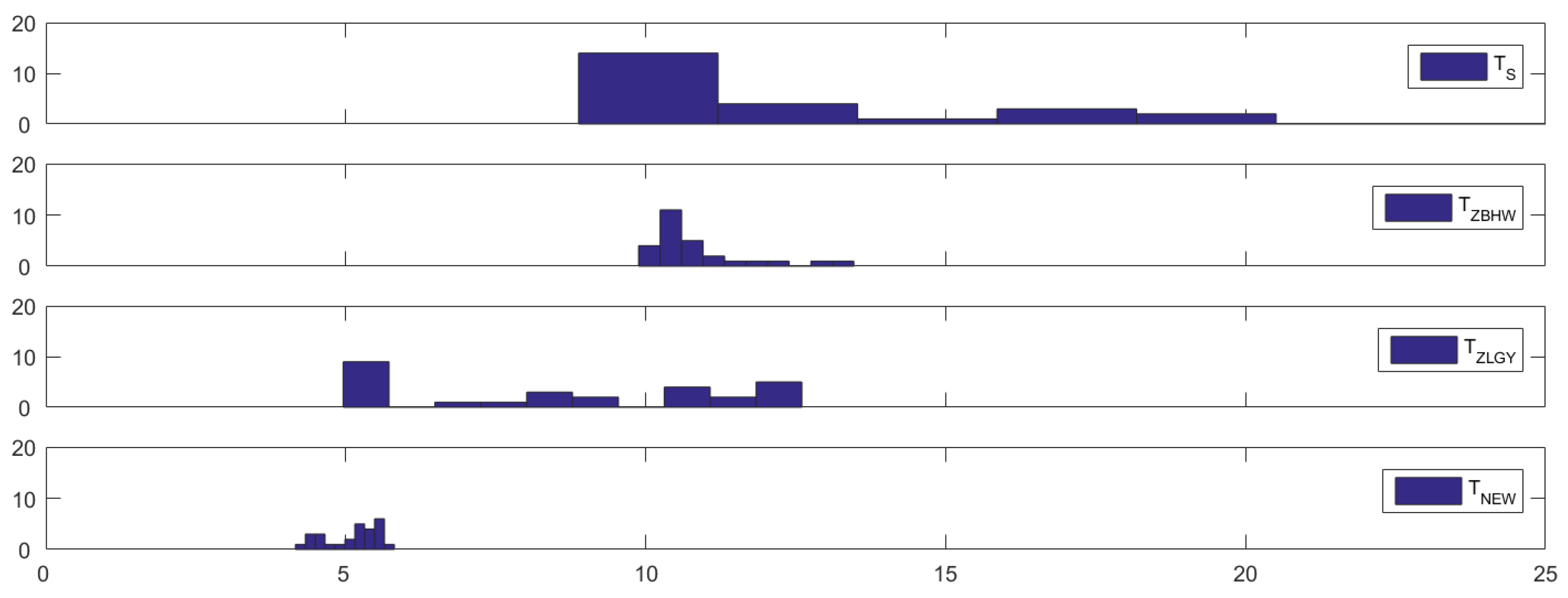
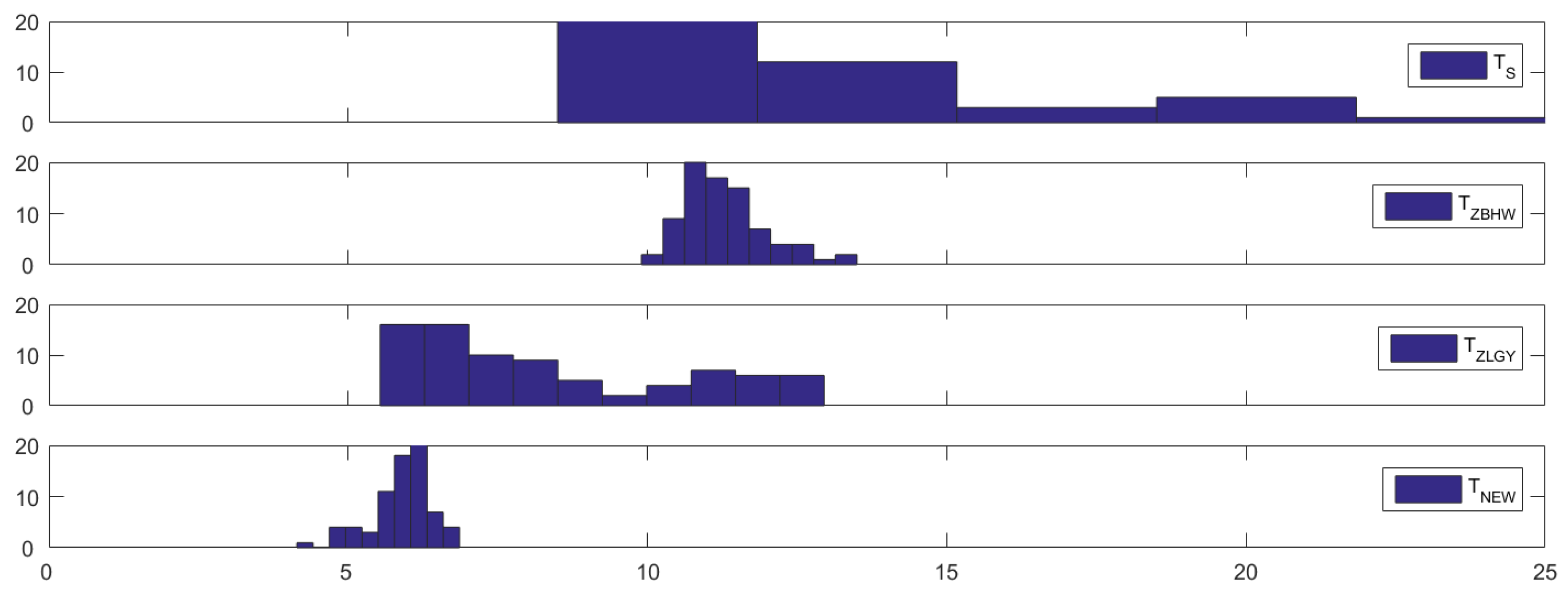
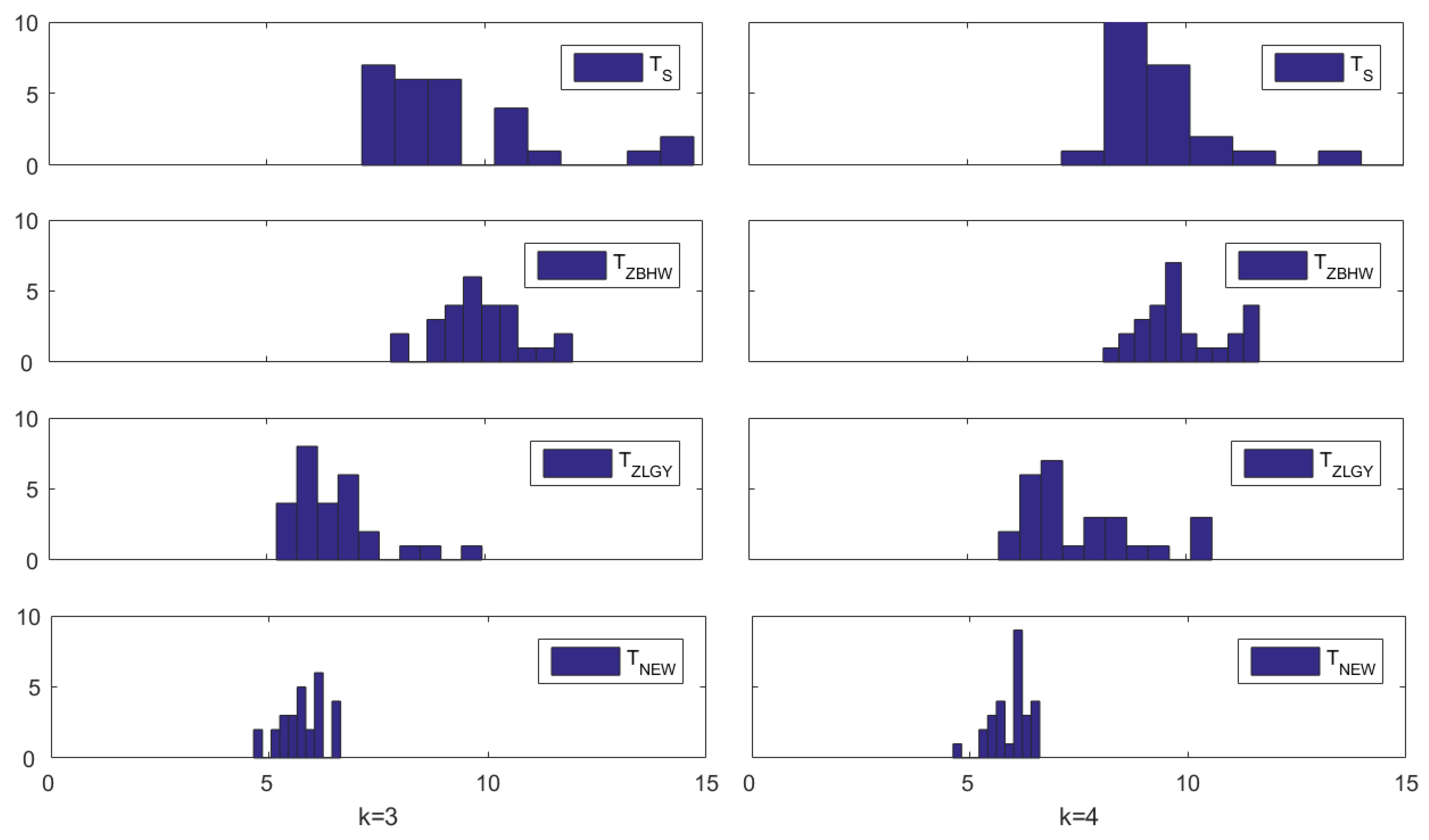
To further illustrate the finite-sample performance of $T_{NEW}$ in terms of size control, we utilize this dataset to calculate the empirical sizes of these test procedures. The empirical size is computed from 10,000 runs. Building upon the testing results provided in Table 6, where we have established that the first three quarters share the same covariance matrix, we proceed to calculate their empirical sizes based on the first two quarters ($k=2$) and the first three quarters ($k=3$). The procedures are outlined as follows: in each run, we randomly partition the $16k$ samples from the first k quarters into k sub-groups of equal size and then compute the p-values to assess the equality of covariance structures among the k sub-groups. The empirical size is determined as the proportion of times the p-value is smaller than the nominal level ${\alpha }^{*}=5\%$ across the 10,000 independent runs.

Table 7. Empirical sizes (%) of the financial dataset with the nominal level ${\alpha }^{*}=5\%$.

k	${\mathit{T}}_{\mathit{S}}$	${\mathit{T}}_{\mathit{ZBHW}}$	${\mathit{T}}_{\mathit{ZLGY}}$	${\mathit{T}}_{\mathit{NEW}}$
2	39.29	21.01	12.37	5.73
3	48.16	33.89	24.25	6.15

presents the empirical sizes of the four tests: $T_S$, $T_{ZBHW}$, $T_{ZLGY}$, and $T_{NEW}$. It is evident from this table that $T_{NEW}$ exhibits significantly improved level accuracy compared to the other three tests, which tend to be quite liberal. This finding aligns with the conclusions drawn from the simulation studies presented in Section 3.

5. Concluding Remarks

In this paper, we introduce and investigate a normal-reference test for the k-sample equal-covariance matrix testing problem, particularly tailored for high-dimensional data. Several existing tests necessitate strong assumptions or conditions, rendering them excessively liberal. Addressing this concern, under certain regularity conditions and null hypothesis, we establish that our proposed test statistic and a chi-square-type mixture share the same limiting distribution. This equivalence permits us to approximate the null distribution of our test statistic without solely relying on the normal approximation. Instead, we leverage the distribution of the chi-square-type mixture for this purpose, ensuring more reliable results and mitigating potential issues associated with the normal approximation, such as unreliable p-values or incorrect rejection rates. Furthermore, we utilize the three-cumulant matched chi-square-approximation proposed by [13] to approximate the distribution of the chi-square-type mixture, with parameters consistently estimated from the data. We apply our methodology to a financial dataset encompassing various sectors across multiple countries during a financial crisis, showcasing the efficacy of our approach in detecting potential financial contagion.

References

1. Dornbusch, R.; Park, Y.C.; Claessens, S. Contagion: Understanding How It Spreads. World Bank Res. Obs. 2000, 15, 177–197. [Google Scholar] [CrossRef]
2. King, M.A.; Wadhwani, S. Transmission of Volatility between Stock Markets. Rev. Financ. Stud. 1990, 3, 5–33. [Google Scholar] [CrossRef]
3. Bekaert, G.; Harvey, C.; Ng, A. Market Integration and Contagion. J. Bus. 2005, 78, 39–69. [Google Scholar] [CrossRef]
4. Corsetti, G.; Pericoli, M.; Sbracia, M. Some contagion, some interdependence: More pitfalls in tests of financial contagion. J. Int. Money Financ. 2005, 24, 1177–1199. [Google Scholar] [CrossRef]
5. Duan, J.C.; Sun, J.; Wang, T. Multiperiod corporate default prediction A forward intensity approach. J. Econom. 2012, 170, 191–209. [Google Scholar] [CrossRef]
6. Li, J.; Chen, S.X. Two sample tests for high-dimensional covariance matrices. Ann. Stat. 2012, 40, 908–940. [Google Scholar] [CrossRef]
7. Cai, T.; Liu, W.; Xia, Y. Two-Sample Covariance Matrix Testing and Support Recovery in High-Dimensional and Sparse Settings. J. Am. Stat. Assoc. 2013, 108, 265–277. [Google Scholar] [CrossRef]
8. Wang, J.; Zhu, T.; Zhang, J.T. Two-sample test for high-dimensional covariance matrices: A normal-reference approach. J. Multivar. Anal. 2024, 204, 105354. [Google Scholar] [CrossRef]
9. Schott, J.R. A test for the equality of covariance matrices when the dimension is large relative to the sample sizes. Comput. Stat. Data Anal. 2007, 51, 6535–6542. [Google Scholar] [CrossRef]
10. Zhang, C.; Bai, Z.; Hu, J.; Wang, C. Multi-sample test for high-dimensional covariance matrices. Commun. Stat.—Theory Methods 2018, 47, 3161–3177. [Google Scholar] [CrossRef]
11. Zheng, S.; Lin, R.; Guo, J.; Yin, G. Testing homogeneity of high-dimensional covariance matrices. Stat. Sin. 2020, 30, 35–53. [Google Scholar] [CrossRef]
12. Zhang, J.T.; Zhu, T. A new normal reference test for linear hypothesis testing in high-dimensional heteroscedastic one-way MANOVA. Comput. Stat. Data Anal. 2022, 168, 107385. [Google Scholar] [CrossRef]
13. Zhang, J.T. Approximate and Asymptotic Distributions of Chi-Squared-Type Mixtures With Applications. J. Am. Stat. Assoc. 2005, 100, 273–285. [Google Scholar] [CrossRef]
14. Wang, R.; Xu, W. An approximate randomization test for the high-dimensional two-sample Behrens–Fisher problem under arbitrary covariances. Biometrika 2022, 109, 1117–1132. [Google Scholar] [CrossRef]
15. Li, W.; Qin, Y. Hypothesis testing for high-dimensional covariance matrices. J. Multivar. Anal. 2014, 128, 108–119. [Google Scholar] [CrossRef]
16. Hu, J.; Li, W.; Liu, Z.; Zhou, W. High-dimensional covariance matrices in elliptical distributions with application to spherical test. Ann. Stat. 2019, 47, 527–555. [Google Scholar] [CrossRef]
17. Yu, X.; Li, D.; Xue, L. Fisher’s Combined Probability Test for High-Dimensional Covariance Matrices. J. Am. Stat. Assoc. 2024, 119, 511–524. [Google Scholar] [CrossRef]
18. Chen, S.X.; Zhang, L.X.; Zhong, P.S. Tests for high-dimensional covariance matrices. J. Am. Stat. Assoc. 2010, 105, 810–819. [Google Scholar] [CrossRef]
19. Westfall, P.H. Kurtosis as peakedness, 1905–2014. RIP. Am. Stat. 2014, 68, 191–195. [Google Scholar] [CrossRef] [PubMed]
20. Bai, Z.D.; Saranadasa, H. Effect of high dimension: By an example of a two sample problem. Stat. Sin. 1996, 6, 311–329. [Google Scholar]
21. Chen, S.X.; Qin, Y.L. A two-sample test for high-dimensional data with applications to gene-set testing. Ann. Stat. 2010, 38, 808–835. [Google Scholar] [CrossRef]
22. Zhang, J.T.; Guo, J.; Zhou, B.; Cheng, M.Y. A simple two-sample test in high dimensions based on L2-norm. J. Am. Stat. Assoc. 2020, 115, 1011–1027. [Google Scholar] [CrossRef]
23. Zhang, J.T.; Zhou, B.; Guo, J.; Zhu, T. Two-sample Behrens–Fisher Problems for High-Dimensional Data: A Normal Reference Approach. J. Stat. Plan. Inference 2021, 213, 142–161. [Google Scholar] [CrossRef]
24. Zhang, J.T.; Zhou, B.; Guo, J. Testing high-dimensional mean vector with applications: A normal reference approach. Stat. Pap. 2022, 63, 1105–1137. [Google Scholar] [CrossRef]
25. Hyodo, M.; Nishiyama, T.; Pavlenko, T. On error bounds for high-dimensional asymptotic distribution of L2-type test statistic for equality of means. Stat. Probab. Lett. 2020, 157, 108637. [Google Scholar] [CrossRef]
26. Székely, G.J.; Rizzo, M.L.; Bakirov, N.K. Measuring and testing dependence by correlation of distances. Ann. Stat. 2007, 35, 2769–2794. [Google Scholar] [CrossRef]
Figure 1. Histograms of the empirical sizes (in %) of T S , T Z B H W , T Z L G Y and T N E W (from top to bottom) in Simulation 1 when k = 3 .
Mathematics 13 00295 g001
Figure 2. Histograms of the empirical sizes (in %) of T S , T Z B H W , T Z L G Y and T N E W (from top to bottom) in Simulation 1 when k = 4 .
Mathematics 13 00295 g002
Figure 3. Histograms of the empirical sizes (in %) in Simulation 2 when k = 3 (left column) and k = 4 (right column).
Mathematics 13 00295 g003