Abstract
This paper investigates the effectiveness of centrality measures for the influence maximization problem in competitive social networks (SNs). We consider a framework, which we call “I-Game” (Influence Game), to conceptualize the adoption of competing products as a strategic game. Firms, as players, aim to maximize the adoption of their products, considering the possible rational choice of their competitors under a competitive diffusion model. They independently and simultaneously select their seeds (initial adopters) using an algorithm from a finite strategy space of algorithms. Since strategies may agree to select similar seeds, it is necessary to include an initial seed tie-breaking rule into the game model of the I-Game. We perform an empirical study in a two-player game under the competitive independent cascade model with three different seed-tie-breaking rules using four real-world SNs. The objective is to compare the performance of centrality-based strategies with some state-of-the-art algorithms used in the non-competitive influence maximization problem. The experimental results show that Nash equilibria vary according to the SN, seed-tie-breaking rules, and budgets. Moreover, they reveal that classical centrality measures outperform the most effective propagation-based algorithms in a competitive diffusion setting in three graphs. We attempt to explain these results by introducing a novel metric, the Early Influence Diffusion (EID) index, which measures the early influence diffusion of a strategy in a non-competitive setting. The EID index may be considered a valuable metric for predicting the effectiveness of a strategy in a competitive influence diffusion setting.
Keywords:
social network; word of mouth marketing; competitive influence diffusion; strategic game; centrality measures MSC:
91D30
1. Introduction
An important research area on social networks (SNs) that has attracted more attention in the last decades is the use of digital word of mouth as a tool for viral marketing. This problem was initially studied as an algorithmic problem in [1] and later formulated as a discrete stochastic optimization problem in [2]. The research focused on exploiting viral effects for Influence Maximization (IM) in SNs. Specifically, considering a stochastic diffusion model that describes how individuals influence each other on a social network and a limited budget k, authors used an algorithm to identify the k most influential initial adopters called seeds. These seeds then convinced friends, colleagues, and family members to adopt the same product, leading to a further cascade of adoptions. Extensive research in the field followed, and many studies have been conducted to determine the most influential initial nodes to maximize the overall number of influenced users in SNs. Propagation-based algorithms and topology-based methods are the two main approaches to the challenge of evaluating nodes’ influence. The former uses Monte Carlo simulation-based algorithms [2,3,4] or reverse influence sampling algorithms [5,6,7]. Although such methods can achieve high solution quality, they are computationally expensive. Topology-based measures, where influential users are identified by their ranking relative to centrality measures such as discounted degree centrality [8] or PageRank centrality [9], avoid this expensive overhead, but the quality of their solutions may be slightly lower or less robust to the network structure.
Furthermore, influence maximization problems have been considered in a competitive environment. Indeed, many real-life situations involve multiple entities competing for influence within a social network. The analysis of the diffusion of competitive influence in social networks (SNs) can be classified based on the interests or concerns of the agents involved. For instance, in word of mouth marketing, competing firms try to maximize the adoption of their products using the same network. In the context of rumor or fake news containment, one agent’s goal is to minimize or block the spread of information from their opponent, while the opponent aims to maximize it.
These scenarios can be analyzed by focusing on identifying the best response to the seed set chosen by the other player or by considering cases where all players adopt a strategic approach. Research in this field has defined several competitive influence diffusion models and studied the properties and algorithmic aspects of the best response function. Notably, prior studies have formulated the following problem: Given a specific competitive influence diffusion model and knowledge of one competitor’s seed set, how can the other competitor determine the optimal seed set of size k to maximize their influence diffusion [10,11]?
In the context of rumor detection, in [12,13,14], authors considered the case of minimizing or blocking the spread of a competitor whose seed set is given and fixed. This problem has also been addressed from a strategic point of view (see, for instance, [15,16]). A recent survey on influence minimization or blocking can be found in [17].
Our contribution examines the scenario where two or more competing firms strategically act by simultaneously trying to maximize the adoption of their products. This competitive situation is modeled as a finite non-cooperative game and analyzed using the concepts of non-dominated strategies and Nash equilibria. By applying game theory, companies can make informed decisions and develop effective marketing strategies to achieve a competitive advantage in product adoption with a limited advertising budget.
More concretely, grounded in non-cooperative game theory, we consider a framework that we call “I-Game” (Influence Game), which models the diffusion of competitive influence in an SN as a strategic game, where firms are players (Throughout the article, we use the terms firms, players, and competitors interchangeably ), their strategies are algorithms or techniques they adopt to select their seed set given a budget k, and their payoffs are the expected number of adopters of their respective product given a competitive influence diffusion model.
In contrast to the best-response problem, directly selecting any possible set of initial seeds for simultaneous choices is impractical. Consequently, this topic has not been extensively explored. Reducing the strategy space to a finite and well-defined set of rules or algorithms for selecting seed sets is essential to address this issue. This approach, also considered in [18,19], is the one we adopt in this paper. A major problem in this kind of model is what decision to make if the seed selection algorithms agree on the nodes they choose. Consequently, a seed selection tie-breaking rule is necessary to resolve seed selection conflicts, and it is incorporated as a relevant part of the I-Game model (the model of [18] can be considered as a particular instance of the I-Game model).
Our main objective is to investigate whether the use of advanced seed selection algorithms, commonly employed in non-competitive environments, offers significant advantages in a competitive environment despite their increased complexity. This assessment aims to help marketing managers determine the most effective approach for their marketing strategies in a competitive environment. To achieve this, we conduct a comprehensive empirical study of relevant instances of the I-Game, comparing the effectiveness of centrality measures as players’ strategies against several highly effective diffusion algorithms.
We study a symmetric two-player game with strategy sets comprising six well-known centrality measures in social networks and three efficient non-competitive algorithms. Additionally, we examine three practical seed selection tie-breaking rules, including the random rule that is commonly used. For diffusion dynamics, we utilize an extension of the IC model [2] to include competitiveness, similar to the one employed in [18]. The expected diffusion under that model determines the players’ payoffs, considering their strategies and the seed selection tie-breaking rule.
We conduct extensive experiments using four real-world SNs that have been widely used as benchmarks in previous research. We perform the dominance analysis and find the Nash equilibrium (NE) strategies to provide empirical results. This includes evaluating the various strategies available to the players for different budgets and seed selection tie-breaking rules.
Our analysis indicates that the efficacy of a strategy in a non-competitive setting may not be maintained when used in a competitive influence diffusion setting. To explain this effect, we present a new metric, the “Early Influence Diffusion Index (EID)”. The EID index offers a quantitative evaluation of a strategy’s efficacy, particularly focusing on the early stages of the diffusion process. The EID index can be used as an a priori indicator to assess the effectiveness of a strategy in competitive environments.
We also observe that the characteristics of the equilibrium outcomes are strongly influenced by the combination of seed selection tie-breaking rules and budget constraints.
In summary, we highlight the scope and potential applications of the findings presented in the paper.
- Primarily, we focus on the area of viral marketing, where various substitute products are being promoted through the same social network. In this context, we propose the “I-Game” framework, which offers a novel perspective on competitive influence diffusion by considering the mutual influence of firms when selecting strategies.
- As a relevant part of the model, we consider three TB rules that try to reflect the way in which seed selection ties would be elucidated at the initial stage. They should be considered as different scenarios in which to evaluate the effectiveness of the strategies under consideration. The analysis focuses on understanding how the scenario created by a particular tie-breaking rule influences the nature of the resulting strategic interactions or situations.
- By selecting the appropriate I-Game instance for a given situation, the performance of a collection of influence maximization algorithms in a competitive environment can be evaluated. This approach provides a deeper insight into how social structure and competitiveness influence the situation under analysis.
- We propose to rely on the I-Game framework to confront the most well-known and commonly used centrality measures by practitioners against some good representatives of sophisticated and computationally expensive influence maximizing state-of-the-art algorithms. It should be noted that our aim is not to be exhaustive in either the selection of centrality measures or influence maximization algorithms.
- Unexpectedly, our results show that the competitive framework has a significant impact on the influence performance of these algorithms.
- We introduce the EID index to explain why competitive superspreaders can perform poorly in a competitive setting. Furthermore, the EID index can be used in some cases to predict the competitive performance of an algorithm.
The rest of the paper is structured as follows. Section 2 is a review of related work. Section 3 presents the non-competitive independent cascade model used as a baseline of our diffusion model and introduces strategic games. Section 4 defines influence strategic games and details our competitive diffusion model and seed selection tie-breaking rules. In Section 5, we perform an empirical study for a two-player game setting and focus on comparing centrality measures with non-competitive state-of-the-art algorithms. We also thoroughly analyze the game results. Section 6 introduces the Early Influence Diffusion Index as a measure of strategy competitiveness. Finally, Section 7 concludes and suggests future work.
2. Related Work
To the best of our knowledge, the work of Carnes et al. [10] is the first attempt to generalize the Independent Cascade model of [2] to a competitive setting. Authors propose two extensions, distance-based and wave propagation models, based on how a node decides which product to adopt when multiple neighbors convince it. The second model describes a scenario in which a node switches to an aware state triggered by all of its active (an active node is a node that has adopted some product) neighbors. The node then randomly adopts the same state as one of its neighbors. The work examines the submodularity of the response function to develop a greedy algorithm for determining the best response, considering that only one player acts strategically.
Goyal and Kearns [20] also propose a switch-and-selection model by defining a general class of switching and selection functions. First, the switching function, which depends on the fraction of active neighbors of the node, gives the probability that it will adopt one of the products. Then, the selection function, which depends on the fraction of its neighbors that have adopted each product, determines which competing products a switched node will choose. They develop a theoretical study of the set of mixed NE, focusing on the price of anarchy and the price of stability to assess the inefficiency of equilibria. In their case, the strategies are given by budget allocations among the nodes, which have no practical applications except for very small, simple networks.
Fotakis et al. [21] use a switch-and-selection competitive model that relies on a threshold model [2] of influence without competition to activate the nodes. They study the submodularity of the response function and the performance of the Nash equilibria of the strategic game they define.
Li et al. [18] also employ a switch-and-selection model related to the wave propagation model of [10]. They consider a simultaneous strategic game where players have finite sets of strategies given by the algorithms or techniques they employ to select their seed set given a budget k. They conclude experimentally that it is possible to “find the optimal strategy for each player regardless of which strategy their rivals adopt”. However, our results show that, in general, no dominant strategies exist. Although our approach is motivated by the work of [18], it generalizes their framework. To fully evaluate the competitive model, we consider a more diversified strategy space to compare the competitive efficiency of centrality-based algorithms with state-of-the-art IM algorithms. Furthermore, we examine how to resolve possible matches in the initial seed selection, which is a significant concern.
In fact, Dubey et al. [22] consider a game to solve this conflict in which players compete for the initial seeds. In [23], authors also consider a seed selection game in which players compete over a finite subset of nodes previously determined by a state-of-the-art IM algorithm.
Ali et al. [24] use reinforcement learning-based models to solve the first-round seed selection, allowing players to select seed nodes in multiple rounds without explicitly knowing the competitor’s decision. Other researchers overlook this problem, opting for a random tie-breaking seed selection rule as in [18], regardless of whether players exhaust their budget. In addition to the random tie-breaking rule, we consider two more realistic rules, assuming that each player is willing to spend their entire budget.
Finally, Budak et al. [25] propose a multi-campaign IC model as a competition between the “bad” and “good” sources. They analyze only the best response to a bad campaign but experimentally observe that centrality-based algorithms are comparable to the costly and effective greedy approach in most cases. As we show, centrality-based algorithms can even outperform IM algorithms in a strategic competitive environment. The EID index we introduce provides an a priori measure to explain this effect.
Table 1 offers a comparison of literature related to competitive influence diffusion.

Table 1.
Comparison of literature reviews.
3. Preliminaries
This section establishes fundamental notations and revisits essential concepts pertinent to our study. We first examine the Independent Cascade (IC) model without competition, then define strategic games and the Nash Equilibrium.
3.1. Social Network Representation and Notations
Social network analysis begins with constructing its formal graph . Graph G consists of a set of vertices or nodes V and a set of arcs . A node in the graph represents a member of the SN (an individual or an organization). An arc connecting two nodes () represents a relationship between the two members of the SN (friendship, colleagues, hyperlink). The relation between nodes can be symmetric, represented by undirected arcs (e.g., being friends on Facebook), or asymmetric, represented by directed arcs (e.g., following someone on ). Given node , we denote the set of in-neighbors of node and the set of its out-neighbors. In non-directed graphs, we refer to the set of neighbors . In addition, each arc can also have a real value to express the influence weight or the influence probability between the two connected nodes.
3.2. Independent Cascade Model
The IC model introduced in [2] is based on models in interacting particle systems and marketing research. Given graph , in the IC model, each arc is associated with a probability of influence to specify the probability for node u to influence its neighbor v. The diffusion process proceeds in discrete time steps, with time ; It starts at step with an initial seed set of active nodes of size k. At each subsequent time step of the diffusion process, node u activated at the previous time step independently makes a single activation attempt on each of its inactive neighbors v. The activation succeeds with probability and fails with probability . The diffusion ends when there are no more active nodes. The key features of the model are that diffusion events along each arc of the graph are independent of each other, and the model is progressive, that is, once active, a node never becomes inactive.
We let be the set of initial seeds, that is, the only active nodes at step . For , we let be the set of nodes influenced in the tth round. Then, for , with probability
If we assume uniform probabilities for the model, i.e., for all , then the activation probability equals
3.3. Strategic Games
Before formulating the competitive diffusion problem as a strategic game, we first recall basic theoretic notions of non-cooperative finite games [26].
Definition 1 (Strategic games).
A strategic game comprises a set of players , where . It is represented by , where is the set of strategies of player i and is its utility or payoff function which assigns to each strategy profile , payoff to player i.
A special case of strategy is a mixed strategy, which is a probability distribution over a set of (pure) strategies S. In this case, the players’ utilities are calculated as expected utilities.
A Nash Equilibrium of is a strategy profile such that, for each and each , .
Intuitively, NE is a steady state in which there is no incentive for any player to unilaterally change his strategy given the strategy of the other players. The interesting aspect of NE is its guaranteed existence in games where players have a finite number of strategies.
Theorem 1
([27]). Every game with a finite number of players in which each player can choose from finitely many pure strategies has at least one NE, possibly in mixed strategies.
The games we consider are symmetric games in which players are indistinguishable, that is, for all and , for all permutations of the player set N and for all strategy profiles .
Theorem 2
([27]). Any finite symmetric game has a symmetric equilibrium, i.e., an NE with , ∀.
4. Competitive Influence Diffusion as a Strategic Finite Game
We now present the problem of competitive influence diffusion in social networks as a strategic game, focusing on the domain of viral marketing. In this context, multiple substitute products are propagated through a single social network. We examine a scenario where no firm has a dominant market position and all firms make decisions independently, without prior knowledge of others’ actions. To ensure fairness in analyzing strategy performance and avoid bias, we assume all firms have identical financial resources, information, and access to advanced algorithms. Additionally, the firms are considered fully rational players, possessing complete information about the presence of competitors, their strategies, and the payoffs for all possible strategy profiles.
In light of the aforementioned considerations, the “influence diffusion strategic game” (I-Game) is defined as a one-shot, simultaneous, symmetric, non-cooperative game with complete information. Its essential elements are as follows:
Social Network: In the graph representation , each arc is associated with vector of influence probabilities for each idea or product. We denote it by .
Players: We let , where , be the set of players who participate with their idea or product to be adopted by the members of the SN. We denote players or agents by .
Strategies: Strategies refer to algorithms or techniques that identify a ranking of preferred nodes for the seeding of the diffusion process. Similarly to the game model of [18], we are not providing a new algorithm specific to the competitive diffusion model, but we consider some of the most well-known strategies already in place in the non-competitive IM field.
Payoffs: Considering the seed sets chosen by the players within their budget limits and under a fixed competitive diffusion model dynamics, the payoff for each player i is determined by the number of nodes that adopt their idea or product at the end of the diffusion process. The goal of each player is to maximize the adoption of his product, taking into account the possible rational choices of the other players.
The optimal solution for all players is determined using the NE solution concept. In particular, we focus on symmetric equilibria, which guarantees equal treatment for all players.
The following sections provide further details on the tie-breaking rules that are employed and the diffusion model that is selected to determine the players’ payoffs.
4.1. Strategies: Seeding Stage
Given a fixed graph , I-Game’s Influence diffusion game evolves in two main stages: A seeding stage and an influence diffusion stage. In the seeding stage, all players independently and simultaneously choose their strategies from the same finite set , , while adhering to a budget constraint.
We use to denote a generic strategy used by player i, where . Typically, strategy produces an ordered sequence of seed candidates , which are eventually random. The sequence exhibits randomness due to the seed selection algorithm, which relies on simulation-based estimations rather than precise computations, or due to situations where ties occur in the node rankings, which may be resolved by implementing a random tie-breaking rule. Thus, the first seeds in this sequence may also be randomly ranked, denoted as . However, if a strategy determines a non-random sequence, we denote it by . Constrained by individual budgets , each player i obtains the first nodes determined by algorithm . This selection process yields the realization of the player’s strategy .
Figure 1 shows the pipeline from strategy selection to final seed set selection.

Figure 1.
Random seed allocation pipeline.
Therefore, the final active seed sets obtained by each player to initiate the diffusion depend on the overlap among their seed sets and some tie-breaking rule employed to assign them to players.
4.1.1. Seed Allocation Algorithms: Tie-Breaking Rules
To investigate the impact of the tie-breaking rule on the game, we examine three distinct models of tie-breaking (TB) rules, namely the Random Tie-Breaking Rule (RTB) [18], the Priority Tie-Breaking Rule (PTB), and the Hybrid Tie-Breaking Rule (HTB). Moreover, the seed allocation algorithms consider whether players decide to replenish lost seeds until they exhaust their full budget or choose to continue with a smaller number of seeds than their budget allows after losing seeds due to ties.
- RTB rule: Each player i selects a set of ordered candidate seeds of size . These are the seeds with which they would like to start their influence diffusion. If there exists a nonempty intersection among sets , i.e., , it implies that more than one player selects certain seeds. Under the RTB rule, a seed selected by more than one player is assigned exclusively to one of the players uniformly at random. A node removed from a player’s initial seed set due to the TB rule is not replaced by another node. Consequently, the actual seed set of each player i, denoted , is at most of size , that is, .
- PTB rule: In seed selection algorithms, nodes are typically ranked based on scores or their order of importance from highest to lowest, with possible ties. Consequently, when player i selects strategy , they are essentially choosing an ordered set of candidate seed sets, denoted by . If a seed occurs in more than one set , , the PTB rule prioritizes the player who assigned the highest ranking to that seed, with tie-breaking based on the node’s position within the seed set. When overlapping seeds have the same rank, they are randomly allocated to one of the players. Unlike the RTB rule, the PTB rule allows each player i, where , to keep selecting seeds until they form a complete independent seed set of size .
- HTB rule: The HTB rule is a hybrid model combining the previous RTB and PTB rules. Once players choose their ordered seeds set , the first round employs the RTB rule to resolve ties among the first seeds in . In the second round, players substitute the seeds lost due to the RTB rule by selecting new ones. If new ties arise during this substitution, the PTB rule is utilized. Players continue this process until they exhaust their budgets, obtaining a total of seeds.
Table 2 illustrates the three TB rules with an example. Since the seed sets obtained after applying the TB rules are random, to distinguish between the active random seed set and a particular realization of that set, we denote the random active seed set of player i as and a particular realization of that set as .
Table 2.
This example illustrates seed allocation for two players with a budget of 3 on an 8-node graph, where Player 1’s algorithm generates the ranked sequence (1, 2, 3, 4, 5, 6, 7, 8) and Player 2’s produces (5, 1, 2, 4, 3, 6, 7, 8). Then, their candidate sets are 1, 2, 3 and 5, 1, 2, respectively. Nodes 1 and 2 are assigned to a player using a TB rule as they appear in both candidate sets. The final sets are shown assuming that in this realization Seeds 1 and 2 are randomly assigned to Players 1 and 2, respectively.
4.1.2. Conceptual Justification of the Tie-Breaking Rules
The three TB rules enable the modeling of potential competitive scenarios without a dominant firm.
The most commonly used RTB rule assumes that when contacted by firms to promote their product, the users do not have any extra incentive to accept one or another product. Hence, their decision of which product to accept is modeled as random. Moreover, firms do not allocate a budget to alternative choices if the initially selected seeds do not accept their product. Fundamentally, the players prioritize having a small number of highly influential nodes, ranked according to strategy, over having a larger number of seeds that may be less influential. However, it is important to mention that RTB is an unrealistic scenario as it is a penalizing rule that can leave one or more competitors without seeds for the competition.
In contrast, under the PTB rule, players are inclined to spend their entire budget to acquire the top-ranked seeds to complete their seed sets, even after losing their initially selected seeds. In particular, assigning a seed to the player who ranks that seed higher could indicate that the player is willing to pay more for it.
Under the HTB rule, firms begin with an initial budget to secure seeds through moderate marketing efforts. If their preferred seeds are lost to competitors, they escalate their efforts by adopting more aggressive marketing strategies to secure their next most desirable choices.
4.2. Diffusion Stage: Payoffs
The competitive diffusion model used in the paper represents a possible extension of the IC model to incorporate a competitive diffusion setting. More specifically, it decomposes the adoption process into two consecutive phases: switching and selection [20]. The switching phase provides the probability that the user adopts one of the products. The selection phase is a decision-making step in which influenced or switched users determine which competing products to choose. We refer to the model as the CIC-SS (Competitive Independent Cascade with Switching and Selection) model.
Separating the propagation of information about the product from its adoption is supported by other previous studies [20,28,29]. Indeed, studies in Social Sciences and Science Management [30] show that the adoption of an innovation or a product often occurs in two stages: awareness and actual adoption. After an individual becomes aware of a type of product or is interested in a type of product, they decide to adopt a specific product based on other factors.
The diffusion process in the CIC-SS model. The diffusion process starts at time with n mutually disjoint seed sets, . Then, the n cascades evolve according to the switching and selection as described below.
- Switching phase: We let denote the set of nodes that are influenced by player in the tth round. Then, for all non-activated nodes , the activation probability equalsIf for all , then the activation probability equals
- Selection phase: If node v is activated, then it selects the product according to the same probabilities. Node with probability proportional to the number of nodes in :where , , denotes the probability for v to adopt the product of player i.
In summary, for a non-influenced node , if there are in-neighbors of v in , then with probability
Definition 2 (Multi-cascade’ Expected spread).
For player i, we use to denote the expected number of active nodes adopting product i under the CIC-SS model starting with seed sets.
Definition 3 (Expected payoffs).
We let be a given influence diffusion strategic game defined by ; the payoff function of the game equals
where , is the random seed set of player i resulting from some TB rule when the players adopt the strategy profile , where strategy produces an ordered random sequence of seed candidates , , and use budgets .
In (1), beyond the randomization inherent in the stochastic diffusion cascade, we also consider the expectation over the randomness in both the selection of seeds and the randomness introduced by the TB rule.
Remark 1.
We can make the following important remarks:
- Node adoption depends on the status of the in-neighbors activated in the previous step rather than on the activating cascade. Therefore, at each step t, the selection phase breaks the competition between the cascade by giving each product adopted by the neighbors of the newly active node a chance of adoption.
- For every and every , at the end of the propagation, the total number of active nodes depends only on the set . In this case, the overall adoption of competitive cascades, regardless of the product, is similar to the non-competitive cascade when seed set T is used exclusively by one party, i.e., without competition.
- Although it is a non-cooperative game, it should be noted that the interests of the players are not entirely antagonistic. All companies are interested in increasing the demand for their type of product on the social network.
4.3. Solution Concept: Nash Equilibrium
The game is analyzed using the NE solution concept, which evaluates the game based on the assumption that each player’s strategy is the best response to the strategies of the other players. The best response of player i to strategy profile of the other players is strategy that yields them the greatest payoff, that is, for all . Previous research primarily focused on the study of the existence of Pure Nash Equilibria (PNEs) strategies derived from graph topology, rather than on the computation of the NE [31,32]. In [18], the emphasis was on identifying a single NE in pure or mixed strategy for a two-strategy game using the RTB rule. Our approach, however, is to identify and analyze all NEs, considering the different instances of the I-Game framework.
To facilitate the analysis of the different situations that may arise in the game, we simplify the game by eliminating irrelevant strategies, such as strictly dominated strategies. Formally, strategy is strictly dominated if there exists strategy such that , for every profile . As the method of iterated elimination of strictly dominated strategies guarantees the preservation of all strategies that support NE, we adopt this approach to reduce the size of the problem and easily identify the different situations. We also ask for dominant strategies if they exist. These are strategies for player i that yield a better outcome for them regardless of the actions of other players; formally, for every strategy profile , .
Note that we are working with the mixed extension of the influence diffusion game, where mixed strategies are taken into account, and players’ utilities are calculated as expected utilities. As observed in [33], a firm may, in fact, adopt a combination of two or more different pure strategies with some probability. Moreover, in a simultaneous marketing campaign, it is prudent to avoid revealing one’s intended starting point to competitors. Mixed strategies may be used with the objective of creating a necessary uncertainty in the opponent as to the intended course of action.
Figure 2 illustrates the workflow of the I-Game framework. For a given SN, an instance of I-Game is determined by a finite strategy space to include any seed selection algorithm, a TB rule for the seed allocations, and a competitive diffusion model. The final Payoff Matrix is produced after simulating the diffusion with the complete strategy profile. The matrix reduction is conducted to remove any strictly dominated strategies, and then the NE is calculated.
Figure 2.
I-Game framework’s workflow.
5. Centrality Versus State-of-the-Art IM Algorithms: Empirical Study
As mentioned above, one of the main motivations of the paper is to explore the effectiveness of simple topology-based algorithms compared to more advanced state-of-the-art IM algorithms when used in a competitive environment. This comparison aims to assess whether, within a competitive environment, we can attain comparable results using basic algorithms, like selecting influential nodes based on their degree centrality, or if we need to consider more complex and difficult-to-implement algorithms.
For this comparative study, we explore a range of widely used centrality measures [9,34]. The six centrality measures used in our experiments are briefly summarized in Table 3. Each centrality measure captures a distinct idea of the local or global importance of the node. Degree Centrality (DC) highlights the most influential users by their follower count. Closeness Centrality (CC) identifies users who can reach other network members in fewer steps. Katz Centrality (KC) is a generalization of DC, stating that a node is important if it is highly connected to nodes close to other nodes in the graph. Betweenness Centrality (BC) measures the number of times a node acts as a bridge along the shortest path between two other nodes, highlighting users who significantly control or obstruct the flow of information. Eigenvector Centrality (EC) reflects the importance of users who are linked to other important users. PageRank (PC) asserts the importance of a node based on the number of connections it has to other important nodes. PageRank can be seen as the sum of random paths that touch the node u.
Table 3.
Centrality Measure Summary. n is the number of nodes. represents an entry of the adjacency matrix A, i.e., if nodes i and j are connected by an arc and otherwise. is the largest eigenvalue of A. Local centrality measures evaluate the importance of the node, taking into account only information about its nearest neighbors. Global centrality requires complete knowledge of the whole SN structure.
As for the most effective algorithms we use in our study, we consider three state-of-the-art algorithms based on different algorithmic paradigms for the IM problem. Specifically, they are the CELF (Cost-Effective Lazy Forward) algorithm [3], the IMM (Influence Maximization through Martingale) algorithm [7], and the DDH (Degree Discount Heuristic) algorithm [8]. CELF is a Monte Carlo simulation-based algorithm designed to improve the efficiency of the naive greedy algorithm of [2]. It reduces unnecessary simulations by using lazy evaluation based on the submodularity property of the diffusion function. IMM is one of the most advanced Reverse Influence Sampling (RIS) algorithms. It should be noted that the difference between greedy algorithms and reverse sampling algorithms is the running time or the efficiency and not, in general, their effectiveness. DDH is a topology-based measure specifically designed to improve degree centrality effectiveness for the IC diffusion model. The rationale behind the DDH algorithm is that selecting a node as a seed implies probability p of activating its neighbors; thus, it discounts their degrees to lower their rank or selection priority as seeds.
Note that our objective is to compare the performance of simple and widely recognized centrality measures in a competitive context against more advanced, resource-intensive influence maximization algorithms. Rather than attempting to cover every available centrality measure, we strategically select the most familiar and frequently utilized by practitioners. The same reasoning is applied in selecting CELF, which is an enhanced version of the Greedy Hill-Climbing algorithm and IMM. In addition, we consider DDH because it represents a middle ground between centrality measures and propagation-based algorithms CELF and IMM.
In summary, the common strategy space is enumerated as Ψ = {DC, KC, CC, EC, BC, PC, DDH, IMM, CELF}.
5.1. Empirical Setting
To simplify the game, we limit the number of players to two. It is also assumed that each player has an equal budget and thus the ability to select an identical number of seeds. This ensures that the results are not affected by the difference in wealth between the two players.
The experiments run on a server with two 64-bit, 2.9 GHz AMD EPYC 7542 processors and 512GB RAM memory under the Rocky Linux 8.5 Operating System. The diffusion algorithms are implemented in the GNU 8.5.0 version of C++. To determine the most central top-k nodes, we employ the open-source tool Networkit [35]. Our framework interfaces with Gambit software (version 16) to efficiently determine NE solutions [36].
Dataset description. The four representative social networks are as follows: (a) Ca-HepTh is an academic collaboration network extracted from the “High Energy Physics—Theory” subcategory of papers from arxiv.org, with nodes representing authors and arcs representing co-authorship relations; (b) Wiki-Vote contains the Wikipedia voting data from the inception of Wikipedia till January 2008, so nodes in the network represent Wikipedia users, and a directed arc represents who-vote-whom; (c) Epinions is a who-trust-whom online SN of a general consumer review site [37]; for influence spread we use the transpose graph of Epinions; and (d) MIT is a Facebook friendship network at one hundred American colleges and universities at a single point in time [38]. The basic properties of the datasets are summarized in Table 4.
Table 4.
Networks data statistics. The clustering coefficient of a node indicates the likelihood that two randomly chosen friends are also friends. Assortativity measures the tendency of nodes in a complex network to connect with similar nodes. Degree assortativity shows that positive values lead to connections between high-degree nodes and between low-degree nodes, whereas negative values indicate a lack of such connections.
Cascade setting. The setting of CIC-SS encloses the following parameters. The influence matrix is unique and homogeneous for both cascades (). Based on the capacity of diffusion in the SN, the propagation probability for each edge is uniformly set to 0.1 for Ca-HepTh, 0.05 for Wiki-Vote, and 0.01 for Epinions and MIT graphs.
Setting the same diffusion probability and budget for both players allows us to observe how the graph topology, the strategies, the TB rules, and the budget size affect the NE solutions. Note that when using the RTB rule, we obtain an instance similar to the one used in [18], but we run the experiments in a broader setting. The budget ranges from 5, 10, 15 to 20. These values are chosen based on the observation that in the non-competitive diffusion, the spread does not increase significantly for budgets greater than 50 in all four graphs, as shown in Figure 3.
Figure 3.
Expected influence diffusion of the strategies without competition. The legend indicates the spread of the strategies in descending order for high budgets.
5.2. Strategy Space Setting
Our initial assessment evaluates the influence diffusion of strategies in the absence of competition. This examination enables us to better identify the additional effects induced by competition in later analyses.
5.2.1. One Source Spread Analysis
Using the IC model, we employ conventional Monte Carlo simulations to approximate expectations by simulating the propagation process thousands of times.
Figure 3 shows the expected influence achieved by the strategies used in our study without competition across the four graphs.
The simulations validate the efficacy of IMM and CELF. The third strategy yielding the highest expected spread varies based on the graph and budget. Focusing on centrality measures, PC centrality outperforms other centrality measures in many cases. Notably, PC’s spread increases with the budget and surpasses DDH in MIT. To enhance discernibility, Table 5 shows the three strategies with the highest expected spread when the budget varies. Starting from Budget 5, DDH surpasses the spread of DC centrality in all four graphs, validating its superior effectiveness compared to DC. BC has a very low spread in Wiki-Vote and Epinions, whereas it performs well in Ca-HepTh and MIT. This discrepancy is attributed to the structural position of the nodes in these networks. Nodes on the periphery but connecting several clusters can achieve a high betweenness score.
Table 5.
The 3 strategies with the highest expected diffusion for the one source diffusion.
In addition, we could observe that in the MIT graph, we obtain a small marginal gain increase for most of the strategies when the budget exceeds 10. This may be related to the fact that it is a one-component graph, which indicates that all the seeds belong to the same component.
5.2.2. Overlap Between the Seed Sets
The degree of similarity between the seed sets produced by the different algorithms is another important information to consider. Considering the TB rules of the I-Game, we use the Ranked Biased Overlap (RBO) similarity measure [39], which is an intersection-based measure of the ranked similarity between two lists of ranked data.
After a thorough examination of the RBO values outlined in Appendix A (from Figure A1, Figure A2, Figure A3 and Figure A4), we consider a value above 0.70 to represent a substantial similarity between two seed sets. When examining the tables, we observe a significant similarity between the pairs KC, DC and DC, DDH sets across the fours graphs. The seed sets of IMM and CELF differ in Ca-HepTh and MIT, while they show remarkable similarities in Epinions and Wiki-Vote. Interestingly, in the Epinions, IMM and CELF exhibit a great intersection with DC, KC, and CC. There are other sporadic similarities specific to data sets and budgets.
The unordered similarity measurement reveals redundancies among several strategies. In particular, KC and DC are identical unordered sets in Wiki-Vote and Epinions across all budgets. Similarly, the pairs of strategies PC, EC and IMM, CELF demonstrate redundancy in Wiki-Vote for Budget 5. In MIT, DC and DDH are identical for Budgets 5 and 10.
For a more accurate study, duplicate unordered seed sets are not taken into account when the RTB rule is used. The selection process is based on two key criteria: interpretability and computational complexity. For instance, in the event of redundancy, DC is selected over KC, and IMM is preferred over CELF.
5.3. Payoffs: Monte Carlo Estimations
We conducted experiments on 48 game instances, varying the SN, TB rules, and budgets. Each game instance was subjected to a Monte Carlo simulation to estimate the expected payoffs of the players. This was achieved by fixing one player’s strategy and varying the other player’s strategies until all strategy profiles were explored. Therefore, for each pair of strategies , the Monte Carlo simulations ran in two consecutive phases: The seeding phase in which a TB rule determines the active seed sets for each player and the influence diffusion phase.
Depending on the standard error associated with the average payoff value for each graph and strategy, the random seed allocation was repeated between 8000 and 12,000 times. The influence diffusion phase was repeated 1000 times for each seed selection realization. The game instance payoffs were recorded in a bi-matrix.
Note that in our experiments, the seed set’s randomness was solely a result of the TB rules, not the algorithms used to identify the seeds. Indeed, our testing revealed that the IMM algorithm consistently generates identical seed sets, provided that the approximation parameters are unchanged. We assumed that both players would simply use the best-recommended approximation parameters. Regarding centrality measures, DC is the only metric that generates a seed set in which nodes of the same degree occur, but this happens more with nodes of lower degrees, which we ignored for the experiments. Additionally, it is reasonable to presume that the seed set remains consistent across all players, given that the algorithms consistently produce an identical seed set, prioritizing first by degree and subsequently by their id. CELF is the only algorithm that can produce different seed sets. However, running it more than once is impractical due to its excessive running time.
5.4. Experimental Results
We now discuss the results of our experiments. We conduct an analysis to examine how competition impacts the behavior of strategies and investigate the influence of TB rules and budgets on the game’s outcome.
The equilibria obtained for all the game instances described in Section 5.3 are presented in Table A9, Table A10 and Table A11. Results are grouped by networks, TB rules, and budgets. Several interesting observations can be made.
First, we find that the SN, TB rules, and budgets impact the game’s outcome. We can see that changing the TB rule highly impacts the equilibrium solutions strategies and type (symmetric, non-symmetric, pure, and mixed NE). Depending on the budget, the RTB rule leads to a higher number of NE solutions than the PTB or HTB rules. This is due to two factors: the high degree of agreement between the seed selection algorithms in some SN and the fact that the RTB rule does not complete the seed sets of the players. Indeed, RTB is more sensitive to the similarity between the seed set because many centrality measures, for example, agree on seeds but not on their rank. Aligning on a common strategy incurs greater penalties under RTB than PTB or HTB rules, thereby preventing symmetric equilibria in pure strategies. Indeed, we can see that we do not obtain symmetric PNE under the RTB rule, except in MIT and one instance in Ca-hepTh. The PTB rule generally results in a single symmetric equilibrium across all graphs and budgets, with an exception in the Epinions for Budget 20. In Epinions, HTB shows similarity to PTB, but it positions itself between RTB and PTB in the remaining three graphs. Thus, PTB and HTB offer a more feasible and solvable strategy for players, characterized by lesser randomness and requiring less coordination between players.
In addition, our experiments reveal an unexpected result regarding the performance of strategies in competitive scenarios. It appears that strategies that excel in non-competitive environments may not maintain their effectiveness when competition is introduced. It is observed that, with the exception of Epinions, centrality measures outperform the highly effective algorithms, IMM and CELF, in terms of payoff in competitive settings. This raises the question of what characteristics or features enable a seed set to maintain its robustness and continue to perform well in a competitive environment. We show that the EID index can be used to answer the question. However, before exploring this question, we present a range of computational results, such as the best response strategy the players, the dominant strategy, and the NE strategies.
5.4.1. Best Response Strategy, Dominant, and Dominated Strategies
After the iterated elimination of strictly dominated strategies from the bi-matrix of the game instances, our analysis revealed two game models: the 2 × 2 anti-coordination (AC) game and the dominance-solvable (DS) game. In the former, the player’s best response is to play a different strategy from their opponent [40]. Anti-coordination games present different PNEs for the two players and hence different possible payoffs in which one player is given a higher payoff than their opponent. A symmetric mixed strategy also exists for these cases. This game emerged in our experiments using the RTB rule. Conversely, the latter game presents a unique pure NE solution, simplifying the decision-making process. The DS game was often given with PTB or HTB rules. The final submatrices are given in Table A1, Table A2, Table A3, Table A4 and Table A5. The best response is marked in yellow for the first player and in green for the second player. We omit the DS game strategies from the tables, as they are presented in the NE tables (Table A9, Table A10 and Table A11).
We can see that IMM and CELF did not survive after the iterative removal of the strictly dominated strategies, except in the Epinions. This means both IMM and CELF are outperformed by one or more centrality measures and that the best strategy for competitive diffusion is not necessarily the best known in non-competitive settings. Instead, we observe that DDH is surviving the iterated elimination of the strictly dominated strategies in several instances being part of the NE solutions in mixed or pure strategy in Ca-HepTh, Wiki-Vote, and Epinions. This outcome underscores the importance of employing strategic games for seed selection in competitive environments.
Finally, it is worth noting that dominant strategies were only identified in the following instances: IMM in Epinions under HTB for Budgets 5 and 10, and KC in MIT under RTB for Budget 20. These results confirm the limitations we reported on the approach used in [18].
5.4.2. Nash Equilibrium Strategies
We now present the NE strategies for all the instances of the game (Table A8, Table A9, Table A10 and Table A11). There are a total of four different situations. The symmetric equilibrium is unique for all instances of the game. When the equilibrium is attained in symmetric PNEs, it is the unique equilibrium of the game (it is a DS game). Otherwise, when the symmetric equilibrium is attained in mixed strategies, three different situations arise: it is the only equilibrium of the game, there are only two more non-symmetric equilibria in pure strategies, or there are multiple non-symmetric pure and/or mixed equilibria. Note that when an asymmetric PNE exists, there is another one obtained by interchanging players’ roles. The non-symmetric NE occurs exclusively under RTB.
Symmetric pure Nash equilibrium. Applying the RTB rule reveals symmetric PNE in MIT (Table A8) across all budgets and in Ca-HepTh (Table A9) excusively for Budget 20. The PTB rule offers symmetric PNE in MIT, Ca-HepTh, and wiki-Vote (Table A10) for all budgets. However, in Epinions (Table A11), the symmetric PNE is found for budgets different from Budget 5. The HTB rule exhibits symmetric PNE in MIT and Wiki-Vote graphs for all budgets. In Ca-HepTh, the symmetric PNE occurs for Budgets 10, 15, and 20, while in Epinions, it is noted for budgets other than Budget 20.
Symmetric mixed Nash equilibrium. Under the RTB rule, the symmetric mixed NE is found in Ca-hepTh for Budgets 5, 10, and 15. Furthermore, it is present in Wiki-Vote and Epinions across all budgets. The only instance of a symmetric mixed NE for the PTB rule occurs in Epinions with a budget of 20. As for the HTB rule, the symmetric mixed NE is observed specifically in Ca-HepTh for Budget 5 and Epinions for Budget 20.
We can now discuss the important results related to the strategies that appear in the equilibria when efficient propagation-based algorithms face centrality-based strategies.
6. The Early Influence Diffusion Index as a Measure of Competitiveness
Surprisingly, strategies that perform the best in a non-competitive setting do not perform as well in a competitive diffusion setting. To analyze this decrease in efficiency, we introduce the Early Influence Diffusion (EID) index as a measure of the effectiveness of a strategy’s influence diffusion.
6.1. Influence Diffusion Efficiency
The traditional influence maximization (IM) problem focuses exclusively on maximizing the number of influenced users without accounting for the time required to achieve this objective. However, time becomes a critical factor in gaining an advantage over competitors in competitive environments. In such scenarios, companies are concerned not only with maximizing the number of influenced users but also with achieving this as quickly as possible, ideally before competitors can do so.
Based on this observation, we consider a scenario where a strategy is employed by a single player without any competition. We then define the EID index of a strategy to quantify the initial rate at which a message or concept spreads within a specific SN when diffusion is triggered by the seed set determined by the given strategy. The metric involves weighting the timing and extent of the influence diffusion of a strategy. First, for a given SN, strategy , and budget k, the t-hop-based expected influence diffusion, denoted by , defined as the expected number of users adopting a product within t time steps or hops for under the IC model, is obtained. Then, to prioritize the diffusion that occurs in the early stages, we consider a discount factor and aggregate the discounted t-hop-based expected influence diffusion.
Formally, the EID index score of a strategy is defined as follows.
Definition 4 (Early influence diffusion index).
Given a non-competitive influence diffusion model, a fixed budget k and a discount factor , the EID index of strategy ψ is
where is the expected hop-based influence diffusion of the random seed set of size k selected by strategy ψ within t hops.
6.2. Comparing Strategy Early Influence Diffusion Index
As the EID index is based on hop-based expected influence diffusion, we first analyze the hop-based expected influence diffusion of the strategies in the four graphs.
To approximate the hop-based expected influence diffusion of strategy , we use Monte Carlo simulation via breadth-first search to sample the number of nodes activated by different hops of propagation [2]. We take the average of 10,000 Monte Carlo simulations as the expected hop-based influence diffusion, for . At time step , is the classical expected spread of without any time limit.
Figure 4, Figure 5, Figure 6 and Figure 7 show the expected influence diffusion of the strategies for different hops of propagation for fixed Budgets 10 and 20. We show the spread from Step 1 to Step 9 for Ca-HepTh and MIT and from Step 1 to Step 7 for Wiki-Vote and Epinions. We can observe that IMM, CELF, and PC have a starting expected diffusion lower than that of DC or KC in Ca-HepTh, MIT, and Wiki-Vote. However, the opposite situation is found in the Epinions graph for IMM and CELF versus DC or CC. This explains why Epinions is the only SN where IMM and CELF maintain their good performance in a competitive diffusion setting. We can also observe that the time it takes for IMM and CELF to reach the diffusion of the centrality measures depends on the network and the budget used. In Wiki-Vote, IMM takes the lead after four hops for Budget 10, while it needs only three hops for Budget 20. In Ca-HepTh, IMM needs nine hops for Budget 10 and eight hops for Budget 20 to reach diffusion of DDH or DC. MIT is a different case in which IMM stays behind for 13 hops.
Figure 4.
Hop-based influence diffusion in Ca-HepTh.
Figure 5.
Hop-based influence diffusion in MIT.

Figure 6.
Hop-based influence diffusion in Wiki-Vote.
Figure 7.
Hop-based influence diffusion in Epinions.
To assess the EID of the strategies, we do not exhaust the complete cascade when estimating all the indexes involved in our experiments. We establish a stopping rule based on the convergence of the Sum (2). Since , for all , we determine the stopping time , such that
It is also important to note that the discount factor w must be chosen appropriately for the EID index to be used as an effective influence assessment metric. Values of w that are too small give too much weight to the initial diffusion steps, which could lead to uninformative EID indexes that are very similar for all strategies. Conversely, values that are too large could have the opposite effect, resulting in EID indexes that are too closely related to the estimated diffusion of the strategies and do not carry any additional information. In our experiments, we choose a value of to discriminate between the EID indices of the strategies effectively.
Table 6 compares the EID index of DC and IMM in the four datasets.
Table 6.
The EID indices for DC versus IMM for different budgets.
We can observe that the EID index score shows different results for the two strategies based on the SN. In Ca-HepTh, MIT, and Wiki-vote datasets, the EID index for DC clearly surpasses that of IMM, whereas we have the opposite scenario in Epinions. We also observe that the EID index is influenced by the budget. Specifically, in the Epinions graph, DC has a higher EID index than IMM for Budget 5 but a lower EID index for other budgets.
Furthermore, the EID index helps to explain the dominated strategies. We can see that PC, which performed well without competition in Ca-HepTh (Table 5), is dominated in Ca-HepTh, i.e., performs worse than the other strategies. We find that its EID index is the lowest in this SN, but it has one of the highest EID index scores in Wiki-Vote, and consequently, PC is in the NE solutions in this graph. Similarly, IMM and CELF have an equivalent expected diffusion in a non-competitive setting in Ca-HepTh and MIT. However, IMM dominates CELF in both SNs, and the calculation shows a higher EID index of IMM over CELF. We can state that strategies that show a higher EID index score in a non-competitive setting are also more effective in a competitive environment. The EID index indicates that for a strategy to perform well in a competitive setting, it is necessary to be a fast spreader, i.e., a strategy that spreads more at the initial stages of the diffusion. This finding confirms that for good decision-making, we should not limit the strategy space to super-spreaders.
6.3. Discussion
Now, we can provide an intuitive explanation for this important result. In the presence of competing strategy , strategy can lose adopters or nodes for two reasons. First, may lose nodes due to tie-breaking when the two strategies reach the same node simultaneously. Second, competing strategy may have managed to reach and win a node at an earlier time step than . Note that not only loses a particular node, but other nodes connected to that node may also be unreachable. This means that a strategy that spreads more in the early stages of diffusion, that is, a strategy with a higher EID index, is prevented from being blockaded. For example, based on our study of hop-based influence diffusion (Figure 4, Figure 5, Figure 6 and Figure 7), we could observe that in the case of Ca-HepTh, for Budget 10, KC achieves 51.33% of the overall diffusion within five hops, whereas IMM attains 42.28%, and PC only manages to reach 23.93%. For Budget 20, KC achieves 65.36% of their total spread, IMM reaches 49.48%, and PC results in only 35.94%.
In other work, the authors have reported the same experience in which, for example, DC performed better than their greedy algorithm in competition [10,25], but they do not provide an explanation for this behavior. This finding may have important implications for future approaches to the problem of competitive diffusion in SNs.
7. Concluding Remarks
This paper presents I-Game, a game-theoretic framework that models competition among multiple firms to maximize their product diffusion in SN. I-Game is a tool for reasoning about the real-world dynamics of influence competition in SN. It offers firms a computational artifact to optimize their payoff by considering the possible rational choices of their competitors.
The game-theoretic analysis reveals that the game’s outcomes can differ based on elements such as the SN structure, the tie-breaking employed for seed overlap, and budget allocations. In any case, the main finding of the paper is that strategies that yield favorable results in a non-competitive environment may not be the most efficient in a competitive setting. We explain this phenomenon by introducing the EID index, which quantifies the early influence diffusion of a strategy in a non-competitive SN. In conclusion, a strategy that spreads fast might be preferable to one that spreads more.
Our study also shows that the unrealistic RTB rule, which is the most commonly used in the literature, is also impractical. Under this scenario, pure non-symmetric equilibria emerge, and thus coordination problems arise for their implementation.
In relation to the proposed I-Game framework, it is important to consider its potential limitations. We delve into its limitations, as well as its possible extensions.
In order to guarantee impartiality in the analysis of strategy performance, we consider a symmetric scenario. Nevertheless, the I-Game framework can be adapted to accommodate different asymmetries between firms, allowing for the analysis of asymmetric situations.
We limit our simulations and analysis to two players; however, the results obtained can serve as a recommendation on how to act in markets with multiple substitute products in which contests occur between two products at a time. Moreover, it can allow to incorporate in the model bounded rationality, in the sense of [41], where authors adopt the definition of “boundedly rational players” as players who experiment with strategies, observe their payoffs, try other strategies, and grope their way toward a strategy that works well.
In our analysis, we consider known and equal budgets. However, extending the analysis to deal with uncertainty about the available budget deserves attention for future work. There can be two different approaches to studying this situation of incomplete information: to rely on Bayesian games [42] or robust games [43]. In both cases, a discrete set of uncertain budgets is considered for each player. Bayesian games assume a common-knowledge prior distribution over uncertain budgets, while robust games are distribution-free; players only know the set of possible budget values. In the first case, players aim to find Bayesian equilibria, while in the second case they strive for robust equilibria.
Finally, this research could be extended to other diffusion models by considering other instances of the CIC-SS model or the competitive linear threshold model to investigate their effects on game outcomes. It might also be interesting to include more sophisticated centrality measures as strategies in study [44].
Author Contributions
Conceptualization, F.M., E.M., and J.T.; methodology, F.M., E.M., and J.T.; software, F.M.; validation, E.M., and J.T.; formal analysis, F.M., E.M. and J.T.; supervision, E.M., and J.T.; writing—original draft preparation, F.M., E.M., and J.T.; writing—review and editing, F.M., E.M., and J.T. All authors have read and agreed to the published version of the manuscript.
Funding
This research has been supported by I+D+i research project PID2020-116884GB-I00 from the Government of Spain.
Data Availability Statement
The original data used in the study are openly available at “https://snap.stanford.edu/data/ (accessed on 10 January 2022)”.
Conflicts of Interest
The authors declare no conflicts of interest.
Appendix A. Rank-Based Similarity

Figure A1.
RBO similarity in Ca-HepTh.
Figure A1.
RBO similarity in Ca-HepTh.
Figure A2.
RBO similarity in MIT.
Figure A2.
RBO similarity in MIT.
Figure A3.
RBO similarity in Wiki-Vote.
Figure A3.
RBO similarity in Wiki-Vote.


Figure A4.
RBO similarity in Epinions.
Figure A4.
RBO similarity in Epinions.
Appendix B. Bi-Matrix Games
Table A1.
Game models in Ca-HepTh RTB.
Table A1.
Game models in Ca-HepTh RTB.
| k = 5 | KC | CC | AC game | ||||
| KC | 372.42 | 372.33 | 378.42 | 376.14 | |||
| CC | 376.14 | 378.42 | 370.09 | 370.24 | |||
| k = 10 | KC | CC | AC game | ||||
| KC | 390.47 | 390.37 | 390.31 | 397.40 | |||
| CC | 397.40 | 390.31 | 374.31 | 374.86 | |||
| k = 15 | DDH | DC | CC | No PNE | |||
| DDH | 403.98 | 403.86 | 390.36 | 422.72 | 406.95 | 418.19 | |
| DC | 422.72 | 390.36 | 388.43 | 388.50 | 397.30 | 394.70 | |
| CC | 418.19 | 406.95 | 394.70 | 397.30 | 381.62 | 381.02 | |
Table A2.
Game models in Ca-HepTh HTB.
Table A2.
Game models in Ca-HepTh HTB.
| k = 5 | KC | CC | AC game | ||
| KC | 390.45 | 390.45 | 378.37 | 397.48 | |
| CC | 397.48 | 378.37 | 374.45 | 374.45 | |
Table A3.
Game models in Wiki-Vote HTB.
Table A3.
Game models in Wiki-Vote HTB.
| k = 15 | KC | CC | DDH | Unique PNE | |||
| KC | 622.70 | 622.90 | 610.09 | 630.12 | 634.42 | 619.00 | |
| CC | 630.10 | 610.09 | 620.07 | 620.07 | 633.18 | 621.30 | |
| DDH | 619.00 | 634.42 | 621.26 | 633.18 | 639.78 | 639.10 | |
Table A4.
Game models in Epinions PTB.
Table A4.
Game models in Epinions PTB.
| k = 20 | KC | CC | IMM | CELF | ||||||
| KC | 466.15 | 465.63 | 466.75 | 468.36 | 450.26 | 490.76 | 475.72 | 466.94 | ||
| CC | 468.36 | 466.75 | 459.15 | 459.93 | 497.59 | 443.83 | 474.55 | 460.86 | No PNE | |
| IMM | 490.76 | 450.26 | 443.83 | 497.59 | 479.3 | 480.25 | 521.54 | 432.83 | ||
| CELF | 466.94 | 475.72 | 460.86 | 474.55 | 432.83 | 521.54 | 477.7 | 476.26 | ||
Table A5.
Game models in Epinions HTB.
Table A5.
Game models in Epinions HTB.
| k = 20 | KC | CC | IMM | No PNE | |||
| KC | 465.85 | 465.85 | 474.99 | 454.80 | 468.45 | 473.64 | |
| CC | 454.80 | 474.99 | 459.50 | 459.5 | 488.92 | 450.53 | |
| IMM | 473.64 | 468.45 | 450.53 | 488.92 | 479.80 | 479.80 | |
Table A6.
Game models in Epinions RTB.
Table A6.
Game models in Epinions RTB.
| k = 5 | IMM | CELF | DC | EC | No PNE | ||||||||
| IMM | 225.02 | 225.02 | 245.64 | 238.36 | 285.57 | 255.06 | 243.24 | 259.51 | |||||
| CELF | 238.36 | 245.64 | 223.61 | 223.61 | 283.58 | 256.64 | 241.42 | 261.76 | |||||
| DC | 255.06 | 285.57 | 256.64 | 283.58 | 218.38 | 218.38 | 243.59 | 282.32 | |||||
| EC | 259.51 | 243.24 | 261.76 | 241.42 | 282.32 | 243.59 | 217.83 | 217.83 | |||||
| k = 10 | IMM | CELF | DC | CC | EC | ||||||||
| IMM | 297.04 | 297.04 | 306.50 | 309.17 | 344.87 | 286.99 | 338.03 | 318.03 | 342.05 | 329.74 | |||
| CELF | 309.17 | 306.50 | 296.47 | 296.47 | 344.11 | 287.51 | 325.00 | 310.98 | 342.40 | 329.29 | |||
| DC | 286.99 | 344.87 | 287.51 | 344.11 | 291.75 | 291.75 | 295.77 | 333.05 | 343.87 | 361.22 | |||
| CC | 318.03 | 338.03 | 310.98 | 325.00 | 333.05 | 295.77 | 295.20 | 295.20 | 347.19 | 341.77 | |||
| EC | 329.74 | 342.05 | 329.29 | 342.40 | 361.22 | 343.87 | 341.77 | 347.19 | 265.00 | 265.00 | |||
| k = 15 | IMM | CELF | DDH | DC | CC | EC | |||||||
| IMM | 345.17 | 345.97 | 367.47 | 350.03 | 376.30 | 358.45 | 378.88 | 355.89 | 382.61 | 360.52 | 411.41 | 366.82 | |
| CELF | 350.03 | 367.47 | 342.99 | 342.17 | 372.41 | 373.18 | 366.83 | 363.98 | 371.43 | 368.89 | 402.82 | 372.27 | |
| DDH | 358.45 | 376.30 | 373.18 | 372.41 | 335.70 | 335.18 | 347.61 | 340.06 | 379.83 | 376.24 | 403.54 | 369.54 | |
| DC | 355.89 | 378.88 | 363.98 | 366.83 | 340.06 | 347.61 | 335.39 | 334.62 | 371.00 | 370.60 | 401.53 | 372.68 | |
| CC | 360.52 | 382.61 | 368.89 | 371.43 | 376.24 | 379.83 | 370.60 | 371.00 | 338.63 | 338.46 | 404.29 | 377.43 | |
| EC | 366.82 | 411.41 | 372.27 | 402.82 | 369.54 | 403.54 | 372.68 | 401.53 | 377.43 | 404.29 | 296.11 | 296.53 | |
| k = 20 | IMM | CELF | DC | CC | EC | ||||||||
| IMM | 380.10 | 380.90 | 405.88 | 389.22 | 413.46 | 404.78 | 414.97 | 412.29 | 451.81 | 414.63 | |||
| CELF | 389.22 | 405.88 | 377.73 | 376.23 | 402.24 | 411.89 | 413.17 | 423.03 | 443.16 | 419.36 | |||
| DC | 404.78 | 413.46 | 411.89 | 402.24 | 368.28 | 369.83 | 410.68 | 411.04 | 442.56 | 410.41 | |||
| CC | 412.29 | 414.97 | 423.03 | 413.17 | 411.04 | 410.68 | 367.44 | 367.62 | 436.85 | 407.02 | |||
| EC | 414.63 | 451.81 | 419.36 | 443.16 | 410.41 | 442.56 | 407.02 | 436.85 | 326.21 | 325.91 | |||
Table A7.
Game models in Wiki-Vote RTB.
Table A7.
Game models in Wiki-Vote RTB.
| k = 5 | DC | PC | AC game | ||||||
| DC | 562.97 | 562.67 | 556.59 | 569.11 | |||||
| PC | 569.11 | 556.59 | 555.76 | 556.52 | |||||
| k = 10 | DC | PC | EC | No PNE | |||||
| DC | 571.36 | 570.34 | 584.93 | 575.81 | 584.54 | 568.86 | |||
| PC | 575.81 | 584.93 | 579.06 | 579.8 | 581.23 | 588.16 | |||
| EC | 568.86 | 584.54 | 588.16 | 581.23 | 571.45 | 570.11 | |||
| k = 15 | DDH | CC | AC game | ||||||
| DDH | 595.41 | 595.67 | 599.11 | 604.46 | |||||
| CC | 604.46 | 599.11 | 584.78 | 584.61 | |||||
| k = 20 | DDH | DC | CC | PC | |||||
| DDH | 616.85 | 616.62 | 616.58 | 629.41 | 613.95 | 631.33 | 631.26 | 633.77 | |
| DC | 629.41 | 616.58 | 594.59 | 593.63 | 607.67 | 608.98 | 625.01 | 603.33 | |
| CC | 631.33 | 613.95 | 608.98 | 607.67 | 603.31 | 602.48 | 634.27 | 617.76 | |
| PC | 633.77 | 631.26 | 603.33 | 625.01 | 617.76 | 634.27 | 612.87 | 613.49 | |
Appendix C. Nash Equilibrium Strategies
Table A8.
NE strategy solutions in MIT.
Table A8.
NE strategy solutions in MIT.
| Player 1 | Player 2 | Payoff | |||||
| KC | EC | KC | EC | P1 | P2 | ||
| RTB | 5 | 0 | 1 | 0 | 1 | 831.46 | 831.46 |
| 10 | 0 | 1 | 0 | 1 | 832.35 | 832.35 | |
| 15 | 1 | 0 | 1 | 0 | 833.69 | 833.69 | |
| 20 | 1 | 0 | 1 | 0 | 835.05 | 835.05 | |
| PTB | 5 | 0 | 1 | 0 | 1 | 832.23 | 832.23 |
| 10 | 0 | 1 | 0 | 1 | 834.60 | 834.60 | |
| 15 | 0 | 1 | 0 | 1 | 836.95 | 836.95 | |
| 20 | 0 | 1 | 0 | 1 | 839.24 | 839.24 | |
| HTB | 5 | 0 | 1 | 0 | 1 | 832.23 | 832.23 |
| 10 | 0 | 1 | 0 | 1 | 834.60 | 834.60 | |
| 15 | 1 | 0 | 1 | 0 | 837.56 | 837.56 | |
| 20 | 1 | 0 | 1 | 0 | 840.46 | 840.46 | |
Table A9.
NE strategy solutions in Ca-HepTh.
Table A9.
NE strategy solutions in Ca-HepTh.
| Player 1 | Player 2 | Payoff | |||||||||
| DDH | DC | KC | CC | DDH | DC | KC | CC | P1 | P2 | ||
| RTB | 5 | 0 | 0 | 1 | 0 | 0 | 0 | 0 | 1 | 379.03 | 375.54 |
| 0 | 0 | 0 | 1 | 0 | 0 | 1 | 0 | 375.54 | 379.03 | ||
| 0 | 0 | 0.73 | 0.27 | 0 | 0 | 0.73 | 0.27 | 374.20 | 374.20 | ||
| 10 | 0 | 0 | 1 | 0 | 0 | 0 | 0 | 1 | 390.31 | 397.40 | |
| 0 | 0 | 0 | 1 | 0 | 0 | 1 | 0 | 397.40 | 390.31 | ||
| 0 | 0 | 0.69 | 0.31 | 0 | 0 | 0.69 | 0.31 | 390.39 | 390.39 | ||
| 15 | 0.16 | 0.64 | 0 | 0.20 | 0.16 | 0.64 | 0 | 0.20 | 395.90 | 395.90 | |
| 20 | 0 | 1 | 0 | 0 | 0 | 1 | 0 | 0 | 404.30 | 404.30 | |
| Player 1 | Player 2 | Payoff | |||||||||
| DDH | DC | KC | CC | DDH | DC | KC | CC | P1 | P2 | ||
| PTB | 5 | 0 | 0 | 1 | 0 | 0 | 0 | 1 | 0 | 390.54 | 390.54 |
| 10 | 0 | 1 | 0 | 0 | 0 | 1 | 0 | 0 | 404.35 | 404.35 | |
| 15 | 1 | 0 | 0 | 0 | 1 | 0 | 0 | 0 | 442.65 | 442.65 | |
| 20 | 1 | 0 | 0 | 0 | 1 | 0 | 0 | 0 | 467.50 | 467.50 | |
| HTB | 5 | 0 | 0 | 1 | 0 | 0 | 0 | 0 | 1 | 378.37 | 397.48 |
| 0 | 0 | 0 | 1 | 0 | 0 | 1 | 0 | 397.48 | 378.37 | ||
| 0 | 0 | 0.36 | 0.64 | 0 | 0 | 0.36 | 0.64 | 382.69 | 382.69 | ||
| 10 | 0 | 1 | 0 | 0 | 0 | 1 | 0 | 0 | 404.35 | 404.35 | |
| 15 | 1 | 0 | 0 | 0 | 1 | 0 | 0 | 0 | 442.65 | 442.65 | |
| 20 | 1 | 0 | 0 | 0 | 1 | 0 | 0 | 0 | 467.50 | 467.50 | |
Table A10.
NE strategy solutions in Wiki-Vote.
Table A10.
NE strategy solutions in Wiki-Vote.
| Player 1 | Player 2 | Payoff | |||||||||||||
| DDH1 | DC | KC | CC | EC | PC | DDH | DC | KC | CC | EC | PC | P1 | P2 | ||
| RTB | 5 | 0 | 1 | 0 | 0 | 0 | 0 | 0 | 0 | 0 | 0 | 0 | 1 | 556.55 | 569.15 |
| 0 | 0 | 0 | 0 | 0 | 1 | 0 | 1 | 0 | 0 | 0 | 0 | 569.15 | 556.55 | ||
| 0 | 0.03 | 0 | 0 | 0 | 0.97 | 0 | 0.03 | 0 | 0 | 0 | 0.97 | 556.75 | 556.75 | ||
| 10 | 0 | 0.73 | 0 | 0 | 0 | 0.27 | 0 | 0.73 | 0 | 0 | 0 | 0.27 | 575.20 | 575.20 | |
| 0 | 0.54 | 0 | 0 | 0.46 | 0 | 0 | 0.27 | 0 | 0 | 0 | 0.73 | 582.64 | 577.20 | ||
| 0 | 0.27 | 0 | 0 | 0 | 0.73 | 0 | 0.54 | 0 | 0 | 0.46 | 0 | 577.20 | 582.64 | ||
| 15 | 1 | 0 | 0 | 0 | 0 | 0 | 0 | 0 | 0 | 1 | 0 | 0 | 597.95 | 605.62 | |
| 0 | 0 | 0 | 1 | 0 | 0 | 1 | 0 | 0 | 0 | 0 | 0 | 605.62 | 597.95 | ||
| 0.56 | 0 | 0 | 0.44 | 0 | 0 | 0.56 | 0 | 0 | 0.44 | 0 | 0 | 596.59 | 596.59 | ||
| 20 | 0 | 0 | 0 | 0 | 0 | 1 | 0 | 0 | 0 | 1 | 0 | 0 | 615.17 | 636.87 | |
| 0 | 0 | 0 | 1 | 0 | 0 | 0 | 0 | 0 | 0 | 0 | 1 | 636.87 | 615.17 | ||
| 0.21 | 0 | 0 | 0.50 | 0 | 0.29 | 0.21 | 0 | 0 | 0.50 | 0 | 0.29 | 618.80 | 618.80 | ||
| 0.86 | 0 | 0 | 0 | 0 | 0.14 | 0 | 0 | 0 | 0.91 | 0 | 0.09 | 614.98 | 632.53 | ||
| 0 | 0 | 0 | 0.91 | 0 | 0.09 | 0.86 | 0 | 0 | 0 | 0 | 0.14 | 632.53 | 614.98 | ||
| PTB | 5 | 0 | 1 | 0 | 0 | 0 | 0 | 0 | 1 | 0 | 0 | 0 | 0 | 570.70 | 570.70 |
| 10 | 0 | 0 | 0 | 1 | 0 | 0 | 0 | 0 | 0 | 1 | 0 | 0 | 602.87 | 602.87 | |
| 15 | 0 | 0 | 0 | 1 | 0 | 0 | 0 | 0 | 0 | 1 | 0 | 0 | 620.10 | 620.10 | |
| 20 | 0 | 0 | 0 | 1 | 0 | 0 | 0 | 0 | 0 | 1 | 0 | 0 | 637.54 | 637.54 | |
| HTB | 5 | 0 | 1 | 0 | 0 | 0 | 0 | 0 | 1 | 0 | 0 | 0 | 0 | 570.70 | 570.70 |
| 10 | 0 | 0 | 0 | 1 | 0 | 0 | 0 | 0 | 0 | 1 | 0 | 0 | 602.87 | 602.87 | |
| 15 | 1 | 0 | 0 | 0 | 0 | 0 | 1 | 0 | 0 | 0 | 0 | 0 | 639.45 | 639.45 | |
| 20 | 0 | 0 | 1 | 0 | 0 | 0 | 0 | 0 | 1 | 0 | 0 | 0 | 630.27 | 630.27 | |
Table A11.
NE strategy solutions in Epinions.
Table A11.
NE strategy solutions in Epinions.
| Player 1 | Player 2 | Payoff | |||||||||||||||
| IMM | CELF | DDH | DC | KC | CC | EC | IMM | CELF | DDH | DC | KC | CC | EC | P1 | P2 | ||
| RTB | 5 | 0.28 | 0.12 | 0 | 0.15 | 0 | 0 | 0.44 | 0.28 | 0.12 | 0 | 0.15 | 0 | 0 | 0.44 | 244.68 | 244.68 |
| 0.46 | 0 | 0 | 0.13 | 0 | 0 | 0.41 | 0 | 0.56 | 0 | 0.09 | 0 | 0 | 0.34 | 248.56 | 245.56 | ||
| 0 | 0.56 | 0 | 0.90 | 0 | 0 | 0.34 | 0.46 | 0 | 0 | 0.13 | 0 | 0 | 0.41 | 245.56 | 248.56 | ||
| 10 | 0 | 0 | 0 | 0 | 0 | 1 | 0 | 0 | 0 | 0 | 0 | 0 | 0 | 1 | 347.19 | 341.77 | |
| 0 | 0 | 0 | 0 | 0 | 0 | 1 | 0 | 0 | 0 | 0 | 0 | 1 | 0 | 341.77 | 347.19 | ||
| 0.37 | 0.18 | 0 | 0 | 0 | 0.23 | 0.22 | 0.37 | 0.18 | 0 | 0 | 0 | 0.23 | 0.22 | 318.26 | 318.26 | ||
| 0 | 0 | 0 | 0 | 0 | 0.95 | 0.05 | 0.88 | 0 | 0 | 0 | 0 | 0 | 0.12 | 321.66 | 338.21 | ||
| 0.88 | 0 | 0 | 0 | 0 | 0 | 0.12 | 0 | 0 | 0 | 0 | 0 | 0.95 | 0.05 | 338.21 | 321.66 | ||
| 0.59 | 0 | 0 | 0 | 0 | 0.21 | 0.20 | 0 | 0.69 | 0 | 0 | 0 | 0.10 | 0.21 | 316.95 | 318.91 | ||
| 0 | 0.69 | 0 | 0 | 0 | 0.10 | 0.21 | 0.59 | 0 | 0 | 0 | 0 | 0.21 | 0.20 | 318.91 | 316.95 | ||
| 15 | 1 | 0 | 0 | 0 | 0 | 0 | 0 | 0 | 0 | 0 | 0 | 0 | 0 | 1 | 410.20 | 368.01 | |
| 0 | 0 | 0 | 0 | 0 | 0 | 1 | 1 | 0 | 0 | 0 | 0 | 0 | 0 | 368.01 | 410.20 | ||
| 0.57 | 0 | 0.17 | 0 | 0 | 0.16 | 0.1 | 0.57 | 0 | 0.17 | 0 | 0 | 0.16 | 0.1 | 362.76 | 362.76 | ||
| 0.18 | 0 | 0 | 0 | 0 | 0.82 | 0 | 0.11 | 0 | 0.89 | 0 | 0 | 0 | 0 | 372.80 | 377.24 | ||
| 0.11 | 0 | 0.89 | 0 | 0 | 0 | 0 | 0.18 | 0 | 0.82 | 0 | 0 | 0 | 0 | 377.24 | 372.80 | ||
| 0.22 | 0 | 0.74 | 0 | 0 | 0.04 | 0 | 0.33 | 0 | 0 | 0 | 0 | 0.20 | 0.66 | 370.12 | 369.12 | ||
| 0.33 | 0 | 0 | 0 | 0 | 0.02 | 0.66 | 0.22 | 0 | 0.74 | 0 | 0 | 0.04 | 0 | 369.12 | 370.12 | ||
| 20 | 1 | 0 | 0 | 0 | 0 | 0 | 0 | 0 | 0 | 0 | 0 | 0 | 0 | 1 | 451.26 | 415.31 | |
| 0 | 0 | 0 | 0 | 0 | 0 | 1 | 1 | 0 | 0 | 0 | 0 | 0 | 0 | 415.31 | 451.26 | ||
| 0.44 | 0.02 | 0 | 0.20 | 0 | 0.24 | 0.1 | 0.44 | 0.02 | 0 | 0.20 | 0 | 0.24 | 0.1 | 403.29 | 403.29 | ||
| 0 | 0.65 | 0 | 0.08 | 0 | 0.21 | 0.06 | 0.47 | 0 | 0 | 0.19 | 0 | 0.24 | 0.1 | 403.31 | 410.76 | ||
| 0.47 | 0 | 0 | 0.19 | 0 | 0.24 | 0.1 | 0 | 0.65 | 0 | 0.08 | 0 | 0.21 | 0.06 | 410.76 | 403.31 | ||
| PTB | 5 | 1 | 0 | 0 | 0 | 0 | 0 | 0 | 1 | 0 | 0 | 0 | 0 | 0 | 0 | 297.04 | 297.04 |
| 10 | 1 | 0 | 0 | 0 | 0 | 0 | 0 | 1 | 0 | 0 | 0 | 0 | 0 | 0 | 380.10 | 380.10 | |
| 15 | 1 | 0 | 0 | 0 | 0 | 0 | 0 | 1 | 0 | 0 | 0 | 0 | 0 | 0 | 435.30 | 435.30 | |
| 20 | 0.06 | 0 | 0 | 0 | 0.41 | 0.53 | 0 | 0.06 | 0 | 0 | 0 | 0.41 | 0.53 | 0 | 465.30 | 465.30 | |
| HTB | 5 | 1 | 0 | 0 | 0 | 0 | 0 | 0 | 1 | 0 | 0 | 0 | 0 | 0 | 0 | 297.04 | 297.04 |
| 10 | 1 | 0 | 0 | 0 | 0 | 0 | 0 | 1 | 0 | 0 | 0 | 0 | 0 | 0 | 380.10 | 380.10 | |
| 15 | 1 | 0 | 0 | 0 | 0 | 0 | 0 | 1 | 0 | 0 | 0 | 0 | 0 | 0 | 435.30 | 435.30 | |
| 20 | 0.40 | 0 | 0 | 0 | 0.32 | 0.28 | 0 | 0.40 | 0 | 0 | 0 | 0.32 | 0.28 | 0 | 469.47 | 469.47 | |
References
- Domingos, P.; Richardson, M. Mining the network value of customers. In Proceedings of the Seventh ACM SIGKDD International Conference on Knowledge Discovery and Data Mining, San Francisco, CA, USA, 26–29 August 2001; pp. 57–66. [Google Scholar]
- Kempe, D.; Kleinberg, J.; Tardos, É. Maximizing the spread of influence through a social network. In Proceedings of the Ninth ACM SIGKDD International Conference on Knowledge Discovery and Data mining, Washington, DC, USA, 24–27 August 2003; pp. 137–146. [Google Scholar]
- Leskovec, J.; Krause, A.; Guestrin, C.; Faloutsos, C.; VanBriesen, J.; Glance, N. Cost-effective outbreak detection in networks. In Proceedings of the 13th ACM SIGKDD International Conference on Knowledge Discovery and Data Mining, KDD ’07, San Jose, CA, USA, 12–15 August 2007; pp. 420–429. [Google Scholar]
- Goyal, A.; Lu, W.; Lakshmanan, L.V. Celf++ optimizing the greedy algorithm for influence maximization in social networks. In Proceedings of the 20th International Conference Companion on World Wide Web, Hyderabad, India, 28 March–1 April 2011; pp. 47–48. [Google Scholar]
- Borgs, C.; Brautbar, M.; Chayes, J.; Lucier, B. Maximizing social influence in nearly optimal time. In Proceedings of the Twenty-Fifth Annual ACM-SIAM Symposium on Discrete Algorithms, Portland, OR, USA, 5–7 January 2014; SIAM: Philadelphia, PA, USA, 2014; pp. 946–957. [Google Scholar]
- Tang, Y.; Xiao, X.; Shi, Y. Influence maximization: Near-optimal time complexity meets practical efficiency. In Proceedings of the 2014 ACM SIGMOD International Conference on Management of Data, Snowbird, UT, USA, 22–27 June 2014; pp. 75–86. [Google Scholar]
- Tang, Y.; Shi, Y.; Xiao, X. Influence maximization in near-linear time: A martingale approach. In Proceedings of the 2015 ACM SIGMOD International Conference on Management of Data, Melbourne, Australia, 31 May–4 June 2015; pp. 1539–1554. [Google Scholar]
- Chen, W.; Wang, Y.; Yang, S. Efficient influence maximization in social networks. In Proceedings of the 15th ACM SIGKDD International Conference on Knowledge Discovery and Data Mining, Paris, France, 28 June–1 July 2009; pp. 199–208. [Google Scholar]
- Lü, L.; Chen, D.; Ren, X.L.; Zhang, Q.M.; Zhang, Y.C.; Zhou, T. Vital nodes identification in complex networks. Phys. Rep. 2016, 650, 1–63. [Google Scholar] [CrossRef]
- Carnes, T.; Nagarajan, C.; Wild, S.M.; Van Zuylen, A. Maximizing influence in a competitive social network: A follower’s perspective. In Proceedings of the Ninth International Conference on Electronic Commerce, Minneapolis, MN, USA, 18–22 August 2007; pp. 351–360. [Google Scholar]
- Bharathi, S.; Kempe, D.; Salek, M. Competitive influence maximization in social networks. In Proceedings of the Internet and Network Economics: Third International Workshop, WINE 2007, San Diego, CA, USA, 12–14 December 2007; Proceedings 3. Springer: Berlin/Heidelberg, Germany, 2007; pp. 306–311. [Google Scholar]
- Wen, S.; Jiang, J.; Xiang, Y.; Yu, S.; Zhou, W.; Jia, W. To Shut Them Up or to Clarify: Restraining the Spread of Rumors in Online Social Networks. IEEE Trans. Parallel Distrib. Syst. 2014, 25, 3306–3316. [Google Scholar] [CrossRef]
- Yan, R.; Li, Y.; Wu, W.; Li, D.; Wang, Y. Rumor blocking through online link deletion on social networks. ACM Trans. Knowl. Discov. Data 2019, 13, 1–26. [Google Scholar] [CrossRef]
- Yang, L.; Li, Z.; Giua, A. Containment of rumor spread in complex social networks. Inf. Sci. 2020, 506, 113–130. [Google Scholar] [CrossRef]
- Etesami, S.R.; Başar, T. Complexity of equilibrium in competitive diffusion games on social networks. Automatica 2016, 68, 100–110. [Google Scholar] [CrossRef]
- Tanınmış, K.; Aras, N.; Altınel, İ.K.; Güney, E. Minimizing the misinformation spread in social networks. Iise Trans. 2020, 52, 850–863. [Google Scholar] [CrossRef]
- Zareie, A.; Sakellariou, R. Minimizing the spread of misinformation in online social networks: A survey. J. Netw. Comput. Appl. 2021, 186, 103094. [Google Scholar] [CrossRef]
- Li, H.; Bhowmick, S.S.; Cui, J.; Gao, Y.; Ma, J. GETREAL: Towards realistic selection of influence maximization strategies in competitive networks. In Proceedings of the ACM SIGMOD International Conference on Management of Data, Melbourne, Australia, 31 May–4 June 2015; Association for Computing Machinery: New York, NY, USA, 2015; pp. 1525–1537, ISSN 07308078. [Google Scholar] [CrossRef]
- Lin, S.C.; Lin, S.D.; Chen, M.S. A Learning-based Framework to Handle Multi-round Multi-party Influence Maximization on Social Networks. In Proceedings of the 21th ACM SIGKDD International Conference on Knowledge Discovery and Data Mining, KDD ’15, Sydney, NSW, Australia, 10–13 August 2015; pp. 695–704. [Google Scholar] [CrossRef]
- Goyal, S.; Kearns, M. Competitive Contagion in Networks. In Proceedings of the Forty-Fourth Annual ACM Symposium on Theory of Computing, STOC ’12, New York, NY, USA, 19–22 May 2012; Association for Computing Machinery: New York, NY, USA, 2012; pp. 759–774. [Google Scholar]
- Fotakis, D.; Lykouris, T.; Markakis, E.; Obraztsova, S. Influence maximization in switching-selection threshold models. In Proceedings of the International Symposium on Algorithmic Game Theory, Haifa, Israel, 30 September–2 October 2014; Springer: Berlin/Heidelberg, Germany, 2014; pp. 122–133. [Google Scholar]
- Dubey, P.; Garg, R.; De Meyer, B. Competing for customers in a social network: The quasi-linear case. In Proceedings of the Internet and Network Economics: Second International Workshop, WINE 2006, Patras, Greece, 15–17 December 2006; Proceedings 2. Springer: Berlin/Heidelberg, Germany, 2006; pp. 162–173. [Google Scholar]
- Ansari, A.; Dadgar, M.; Hamzeh, A.; Schlötterer, J.; Granitzer, M. Competitive Influence Maximization: Integrating Budget Allocation and Seed Selection. arXiv 2019, arXiv:1912.12283. [Google Scholar]
- Ali, K.; Wang, C.Y.; Chen, Y.S. Leveraging transfer learning in reinforcement learning to tackle competitive influence maximization. Knowl. Inf. Syst. 2022, 64, 2059–2090. [Google Scholar] [CrossRef]
- Budak, C.; Agrawal, D.; El Abbadi, A. Limiting the spread of misinformation in social networks. In Proceedings of the 20th International Conference on World Wide Web, Hyderabad, India, 28 March–1 April 2011; pp. 665–674. [Google Scholar]
- Başar, T.; Olsder, G.J. Dynamic Noncooperative Game Theory, 2nd ed.; Classics in Applied Mathematics, Society for Industrial and Applied Mathematics (SIAM): Philadelphia, PA, USA, 1999. [Google Scholar]
- Nash Jr, J.F. Equilibrium points in n-person games. Proc. Natl. Acad. Sci. USA 1950, 36, 48–49. [Google Scholar] [CrossRef] [PubMed]
- Borodin, A.; Filmus, Y.; Oren, J. Threshold models for competitive influence in social networks. In Proceedings of the Internet and Network Economics: 6th International Workshop, WINE 2010, Stanford, CA, USA, 13–17 December 2010; Proceedings 6. Springer: Berlin/Heidelberg, Germany, 2010; pp. 539–550. [Google Scholar]
- Lu, W.; Chen, W.; Lakshmanan, L.V.S. From competition to complementarity: Comparative influence diffusion and maximization. Proc. VLDB Endow. 2015, 9, 60–71. [Google Scholar] [CrossRef]
- Kalish, S. A new product adoption model with price, advertising, and uncertainty. Manag. Sci. 1985, 31, 1569–1585. [Google Scholar] [CrossRef]
- Alon, N.; Feldman, M.; Procaccia, A.D.; Tennenholtz, M. A note on competitive diffusion through social networks. Inf. Process. Lett. 2010, 110, 221–225. [Google Scholar] [CrossRef]
- Tzoumas, V.; Amanatidis, C.; Markakis, E. A game-theoretic analysis of a competitive diffusion process over social networks. In Proceedings of the International Workshop on Internet and Network Economics, Singapore, 11–14 December 2012; Springer: Berlin/Heidelberg, Germany, 2012; pp. 1–14. [Google Scholar]
- Easley, D.; Kleinberg, J. Networks, Crowds, and Markets: Reasoning About a Highly Connected World; Cambridge University Press: Cambridge, UK, 2010. [Google Scholar]
- Bloch, F.; Jackson, M.O.; Tebaldi, P. Centrality measures in networks. Soc. Choice Welf. 2023, 61, 413–453. [Google Scholar] [CrossRef]
- Staudt, C.L.; Sazonovs, A.; Meyerhenke, H. NetworKit: A tool suite for large-scale complex network analysis. Netw. Sci. 2016, 4, 508–530. [Google Scholar] [CrossRef]
- McKelvey, R.D.; McLennan, A.M.; Turocy, T.L. Gambit: Software Tools for Game Theory, Version 16.0.2.; 2014. Available online: http://www.gambit-project.org/ (accessed on 13 January 2022).
- Leskovec, J.; Krevl, A. SNAP Datasets: Stanford Large Network Dataset Collection. 2014. Available online: http://snap.stanford.edu/data (accessed on 10 January 2022).
- Rossi, R.; Ahmed, N. The network data repository with interactive graph analytics and visualization. In Proceedings of the AAAI Conference on Artificial Intelligence, Austin, TX, USA, 25–30 January 2015; Volume 29, pp. 4292–4293. [Google Scholar]
- Webber, W.; Moffat, A.; Zobel, J. A similarity measure for indefinite rankings. ACM Trans. Inf. Syst. 2010, 28, 1–38. [Google Scholar] [CrossRef]
- Bramoullé, Y.; López-Pintado, D.; Goyal, S.; Vega-Redondo, F. Network formation and anti-coordination games. Int. J. Game Theory 2004, 33, 1–19. [Google Scholar] [CrossRef]
- Samuelson, L. Bounded rationality and game theory. Q. Rev. Econ. Financ. 1996, 36, 17–35. [Google Scholar] [CrossRef]
- Harsanyi, J.C. Games with Incomplete Information Played by "Bayesian" Players, I-III. Part III. The Basic Probability Distribution of the Game. Manag. Sci. 1968, 14, 486–502. [Google Scholar] [CrossRef]
- Aghassi, M.; Bertsimas, D. Robust game theory. Math. Program. 2006, 107, 231–273. [Google Scholar] [CrossRef]
- Passacantando, M.; Raciti, F. A Variational Inequality Approach to a Class of Network Games with Local Complementarities and Global Congestion. In Proceedings of the Optimization in Artificial Intelligence and Data Sciences; Amorosi, L., Dell’Olmo, P., Lari, I., Eds.; Springer: Cham, Switzerland, 2022; pp. 1–11. [Google Scholar]
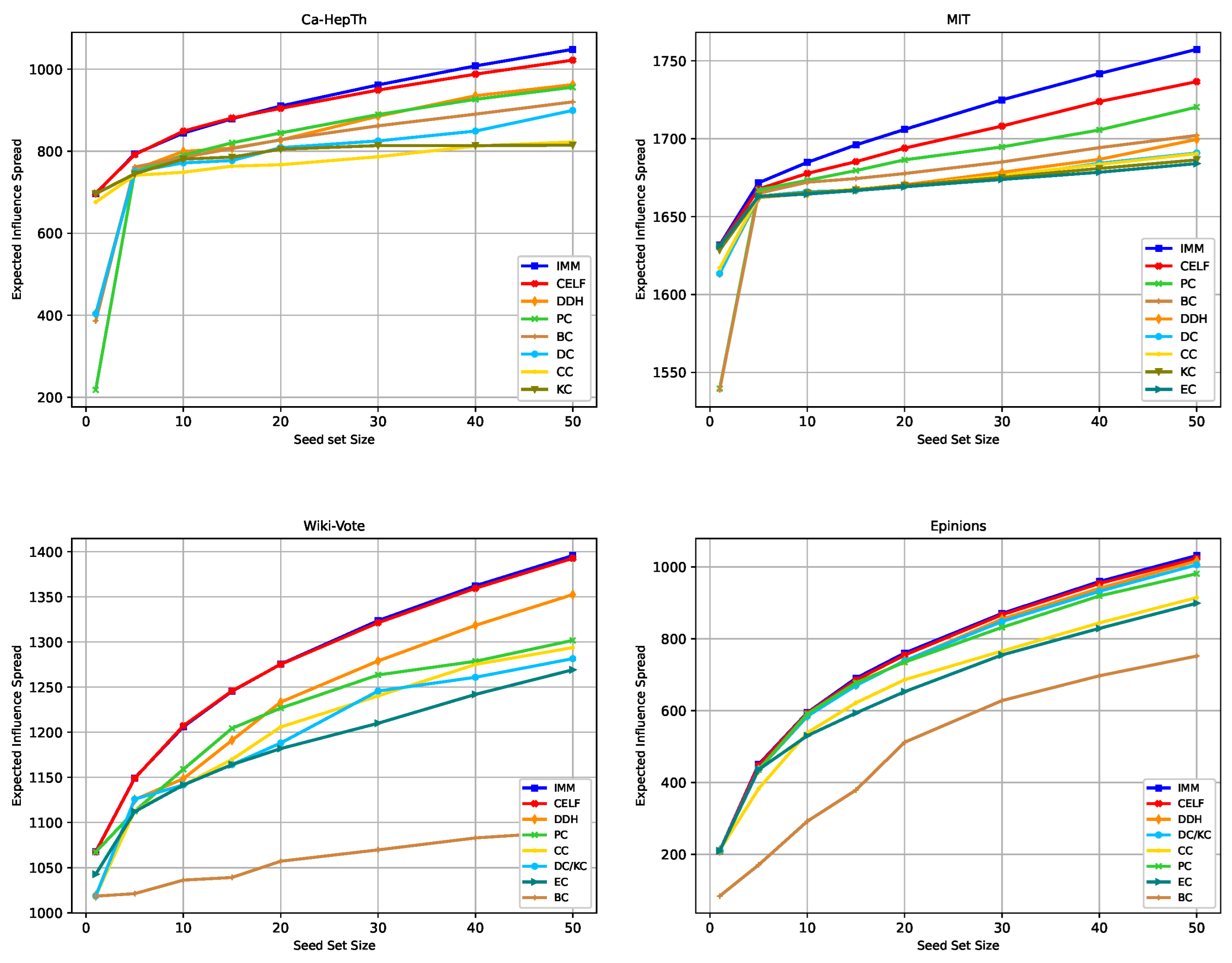
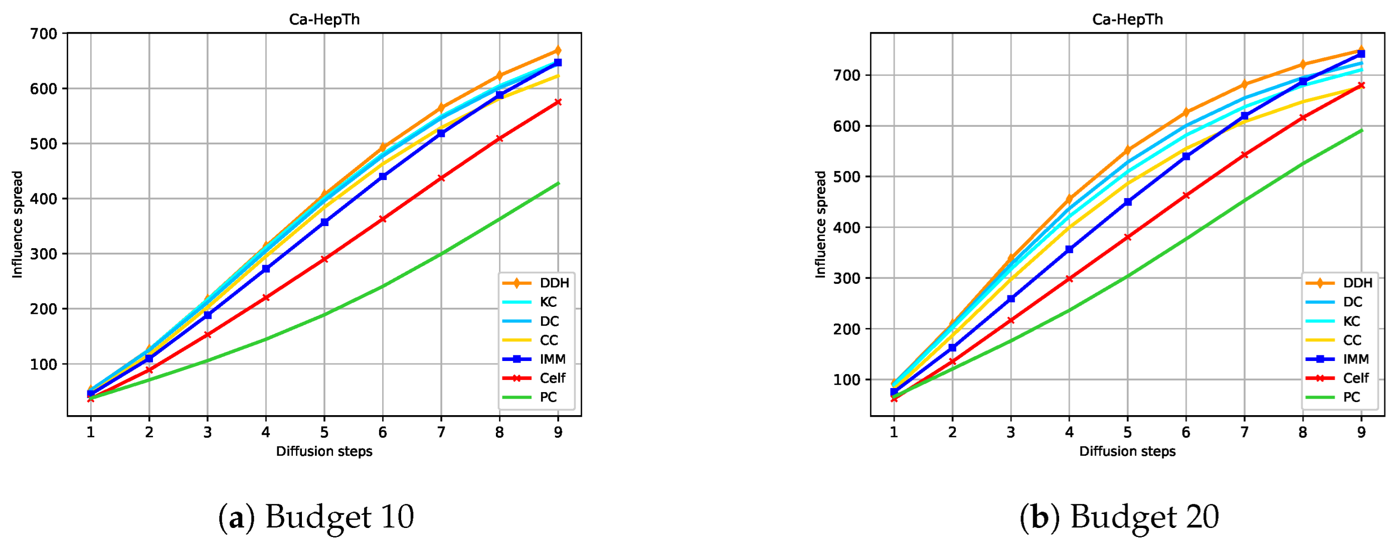
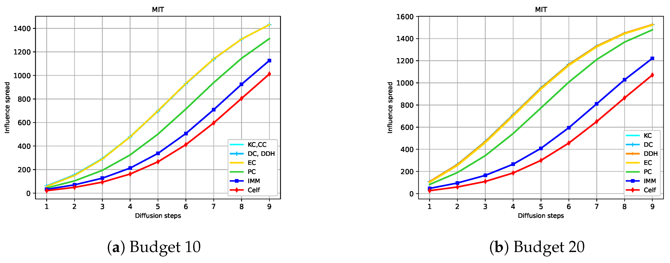
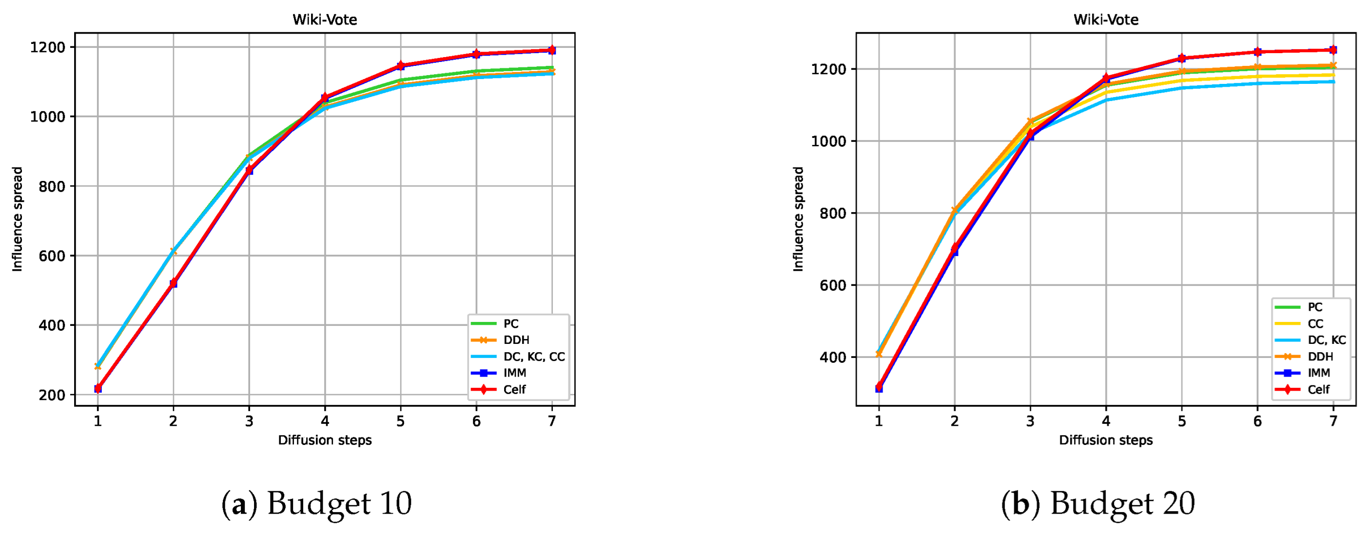

Disclaimer/Publisher’s Note: The statements, opinions and data contained in all publications are solely those of the individual author(s) and contributor(s) and not of MDPI and/or the editor(s). MDPI and/or the editor(s) disclaim responsibility for any injury to people or property resulting from any ideas, methods, instructions or products referred to in the content. |
© 2025 by the authors. Licensee MDPI, Basel, Switzerland. This article is an open access article distributed under the terms and conditions of the Creative Commons Attribution (CC BY) license (https://creativecommons.org/licenses/by/4.0/).