Abstract
In machine learning, the processing of datasets is an unavoidable topic. One important approach to solving this problem is to design some corresponding algorithms so that they can eventually converge to the optimal solution of the optimization problem. Most existing acceleration algorithms exhibit asymptotic convergence. In order to ensure that the optimization problem converges to the optimal solution within the prescribed time, a novel prescribed-time convergence acceleration algorithm with time rescaling is presented in this paper. Two prescribed-time acceleration algorithms are constructed by introducing time rescaling, and the acceleration algorithms are used to solve unconstrained optimization problems and optimization problems containing equation constraints. Some important theorems are given, and the convergence of the acceleration algorithms is proven using the Lyapunov function method. Finally, we provide numerical simulations to verify the effectiveness and rationality of our theoretical results.
Keywords:
exponential prescribed-time convergence; acceleration algorithm; time rescaling; optimization problem; Lyapunov function MSC:
65K10
1. Introduction
Machine learning stands as a predominant approach to addressing numerous artificial intelligence challenges in the present day. It has a wide range of applications across various domains, including but not limited to computer vision, natural language processing, secure communication, and search technologies. With the development of the Internet, dealing with huge datasets has become a topic of concern for scholars. As a result, many requirements are placed on the convergence speed of machine learning, and gradient descent-based algorithms naturally attract attention.
The origins of the earliest accelerated algorithms [1] can be traced to the heavy-ball method proposed by Polyak in 1964. This method achieved a local linear convergence rate through spectral analysis. Since it was difficult to guarantee global convergence for the heavy-ball method, Nesterov later proposed the Nesterov accelerated gradient (NAG) method [2] using estimated sequences in 1983, which reduced the complexity of the classical gradient descent method and showed the worst-case convergence speed of in minimizing smooth convex functions. To further advance the development of the acceleration algorithm, Nesterov proposed methods with a convergence speed of for a class of smooth convex functions that are unconditionally minimized [3]. A universal method for developing optimal algorithms aimed at minimizing smooth convex functions was presented in [4]. Thereafter, the heavy-ball method and the accelerated gradient method attracted the attention of numerous scholars. In 1994, Pierro et al. [5] proposed a method to speed up iterative algorithms for solving symmetric linear complementarity problems. At the same time, Arihiro et al. [6] proposed an enhancement to the error backpropagation algorithm, widely used in multilayer neural networks, by incorporating prediction to improve its speed. However, these methods did not garner significant interest within the machine learning community. It was not until Beck and Teboulle [7] introduced the accelerated proximity gradient (APG) method in 2009, aimed at solving composite optimization problems, including sparse and low-rank models, that the machine learning community began to take significant notice. This method was an extension of the work in [4] and was simpler compared to that in [8]. As it happens, the sparse and low-rank models are common in machine learning. The accelerated proximity gradient (APG) method has been widely recognized in the field of machine learning.
However, one of the drawbacks of the methods based on Nesterov’s method was that they exhibited an oscillatory behavior, which could seriously slow down their convergence speed. Many scholars have made extensive attempts to address this problem. B. O’Donoghue and E. Candès [9] introduced a function restart strategy and a gradient restart strategy to enhance the convergence speed of Nesterov’s method. Further, Nguyen et al. [10] proposed the accelerated residual method, which could be regarded as a finite-difference approximation of the second-order ODE system. The method was shown to be superior to Nesterov’s method and was extended to a large class of accelerated residual methods. These strategies successfully mitigated the oscillatory convergence associated with Nesterov’s method. The convergence of the aforementioned accelerated algorithms is mainly asymptotic, i.e., the solution to the optimization problem or the ODE problem is obtained as time tends to infinity.
It is well known that finite-time convergence has made great progress in dynamical systems, where the convergence time is linked to the system’s initial conditions. In addition, there is another type of convergence: fixed-time convergence. Fixed-time convergence is independent of the initial value and enables the estimation of the upper limit of the settling time without relying on any data regarding the initial conditions. While fixed-time convergence offers numerous benefits for estimating when a process will stop, it cannot establish a straightforward and lucid link between the control parameters and the target maximum stopping time. This frequently results in an overestimation of the stopping time, which, in turn, misrepresents the system’s performance. Additionally, the stopping time cannot be directly adjusted in finite-time or fixed-time convergence scenarios since it is also influenced by the design parameters of other control systems. In order to address the challenge of excessive estimations regarding the stopping time and to reduce the dependence of the stopping time on design parameters, a prescribed-time convergence has been developed [11]. In other words, the system is capable of achieving stability within a predetermined timeframe, irrespective of the initial conditions. It should be highlighted that the integration of prescribed-time convergence with optimization problems is likewise a fascinating area of study [12,13,14].
In practice, many dynamical systems are related to time. Time rescaling is a concept that involves time transformation. Within the realm of non-autonomous dissipative dynamic systems, adjusting the time parameter is a simple yet effective approach to expedite the convergence of system trajectories. As noted in the unconstrained minimization problem in [15,16,17] and the linear constrained minimization problem in [18,19], the time-rescaling parameter has the effect of further increasing the rate of convergence of the objective function values along the trajectory. Balhag et al. [20] developed fast methods for convex unconstrained optimization by leveraging inertial dynamics that combine viscous damping and Hessian-driven damping with time rescaling. In their work [21], Hulett et al. introduced the time-rescaling function, which resulted in improved convergence rates. This achievement can also be considered a further development of the time-rescaling approach that was presented for constrained scenarios in [15,16].
Based on the above facts, we ensure that the optimization problem converges to the optimal solution within the prescribed time, and a novel prescribed-time convergence acceleration algorithm with time rescaling is proposed. A distinctive aspect of this paper is the utilization of time rescaling to integrate the concept of prescribed time with second-order systems for tackling optimization problems. This enables the optimization problem to achieve convergence to the optimal value within the prescribed time. Several second-order systems with respect to time t for unconstrained optimization problems and optimization problems containing equational constraints were presented in [22,23,24,25]. Under these second-order systems, the above optimization problems yielded asymptotic convergence. In contrast to [22,23,24,25], the contributions of this paper are as follows:
(1) We obtain the prescribed-time convergence rate , where , is a positive function, T is the prescribed time, and as t → T, we have
(2) In some cases, the use of time rescaling improves the convergence of the optimization algorithm. So, we use to transform the time t into an integral form, i.e., , where is a continuous positive function. In this way, the second-order system we construct becomes more flexible, and the convergence is improved to a certain extent. We give different and verify the validity of the results with numerical simulations.
In addition, we compare this paper with the literature [15,16,18,20], as shown in Table 1. To simplify, ➀ and ➁ are used to represent smooth and non-smooth objective functions, respectively; ➂, ➃, and ➄ are used to represent the unconstrained optimization problem, the optimization problem with equation constraints, and the structured convex optimization problem, respectively; ➅ is used to represent “Accelerate”; and ➆ and ➇ are used to represent “converge within the prescribed time, i.e., , ” and “asymptotic convergence, i.e., , ”, respectively.

Table 1.
Different algorithmic models.
The subsequent sections of this article are structured as follows. Section 2 provides a concise overview of the fundamental concepts utilized throughout this paper. In Section 3 and Section 4, we design new algorithms that allow unconstrained optimization problems and optimization problems with equational constraints to converge to the optimum within the prescribed time. We give corresponding examples for different time rescalings in Section 5. Numerical simulations are given in Section 6. Conclusions and suggestions for future work are given in Section 7.
2. Preliminaries
Consider the Hilbert space V, and let f:V → R be a properly -strongly convex differentiable smooth function. Furthermore, the space V is equipped with an inner product and the corresponding norm . The notation represents the duality pairing between and V, where is the continuous dual space of V, equipped with the standard dual norm . For simplicity, we consider the real vector space , whose Euclidean norm is denoted as for . For a given function f, let be its optimal point for the optimization problem, and the optimal value is . In addition, the lemmas used in this paper are provided below.
Lemma 1
([23]). For any , we have
Lemma 2
([23]). If f is a μ-strongly convex differentiable function, then for any , where Ω is the domain of definition of f, we have
Assumption 1.
The function is a continuous positive function, i.e., .
Assumption 2.
When holds, let the relationship between t and δ be
i.e., (1) is a time rescaling. And the above equation satisfies that when , holds, where T is a positive number. We have
Also, the inverse function
obtained from the above equation satisfies that when , there is .
Assumption 3.
When holds, let the function
and the above equation satisfy that when there is .
Assumption 4.
In the case of > 0 and (1),
holds.
Assumption 5.
In the case of satisfying > 0, let the function
and the above equation satisfy that when , there is
In [23], for the unconstrained optimization problem
of a smooth function f on the entire space V, the second-order ODE constructed for the optimization problem is
The aforementioned system can be transformed into the following system of first-order ordinary differential equations (ODEs):
Meanwhile,
In [25], the author used primal-dual methods to study the convex optimization problem constrained by linearity
Specifically, when f is a smooth function, the system constructed for the optimization problem containing the equation constraints is
Meanwhile,
Different second-order systems are constructed for the above two types of optimization problems. Then, by introducing different Lyapunov functions, both optimization problems reach asymptotic convergence, i.e., as , there is .
Remark 1.
Under certain conditions, the authors of [26] used the generalized finite-time gain function concerning the variable τ, obtaining that when , there is . The result obtained is also asymptotically convergent. Inspired by the literature [26], we modify the above two systems to obtain that when t → T, there is , where T is the prescribed time.
Remark 2.
Instead of directly giving the second-order system with respect to the variable t, we first use the time rescaling in [23] to construct the system with respect to the variable δ. By establishing the coefficient relationship between the two systems and applying this relationship, we indirectly obtain the second-order system with respect to the variable t.
3. For Unconstrained Optimization Problems
In this subsection, we construct a category of second-order systems designed to address the unconstrained optimization issue (9), ensuring that the solution converges to the optimal outcome within the prescribed time under the influence of these second-order systems.
We consider the unconstrained optimization problem
where , , and f is a -strongly convex differentiable smooth function. Let its optimal solution be .
Based on the ODE theory, which can provide deeper insights into optimization, we aim to design a second-order system of the following form:
where , is a positive function, , , , and
Additionally, our objective is to identify an appropriate such that (9) achieves convergence to the optimal solution within the prescribed time under the influence of Equation (9a,b). Specifically, as , we require that . In order to find the right , we proceed as described below.
Firstly, the variable transformation is used to change the optimization problem (9) into the following equivalent optimization problem (11). The details are given below.
Using the relationship between t and , we can obtain
By substituting (10) into (9), we obtain the optimization problem
which is equivalent to (9), where y = y(), , and f is a -strongly convex differentiable smooth function. The optimal solution of the optimization problem (11) is also .
Secondly, under certain conditions, a second-order system is constructed to solve the optimization problem (11), so that (11) converges asymptotically to the optimal solution under the action of the system. The details are given below.
Inspired by [23], a second-order system is constructed for the optimization problem (11) as follows:
where , , and are positive functions, , and . Additionally, we have the equation
Next, by applying the variable transformation
along with (2), (9a,b) and (11a,b), we obtain
Finally, after analyzing (9a,b) and (11a,b), we find that
By substituting Assumption 4 into the above equation, we find that
holds. Therefore, for the optimization problem (11), we use to construct a second-order system (14a,b):
where , is a positive function, and , . Additionally, we have the equation
Next, we show that the optimization problem (11) converges asymptotically to the optimal value under system (14a,b), where satisfies Assumptions 1–4.
Theorem 1.
The optimization problem (11) converges asymptotically to the optimal value under system (14a,b), where satisfies Assumptions 1–4.
Proof.
We construct the Lyapunov function as follows:
Differentiating the above equation with respect to yields
By substituting (14a,b) into the above equation and using Lemmas 1 and 2, we obtain
Furthermore, we have
By applying Assumption 3 to the above equation, we can obtain . So, as , we can obtain . □
In summary, we can ensure that the optimization problem (11) asymptotically converges to the optimal solution by using the second-order system (14a,b) derived from Assumptions 1–4. Although we can obtain the expression of from Assumption 4, substituting this into system (9a,b) does not guarantee that the optimization problem (9) converges to the optimal solution within the prescribed time T.
Thirdly, under certain conditions, a second-order system is constructed to solve the optimization problem (9) so that (9) converges to the optimal solution within the prescribed time T.
Theorem 2.
When and satisfy Assumptions 1–5, the optimization problem (9) can converge to the optimal solution within the prescribed time under the action of system (9a,b).
Proof.
From Assumptions 1–4, we can derive . In addition, it is known from Assumption 2 that as , and vice versa.
For (9a,b), the adaptive Lyapunov function is
and (16) takes advantage of the fact that is a positive function. Differentiating the above equation with respect to t yields
By substituting (9a,b) into the above equation and using Lemmas 1 and 2, we obtain
Further, we have
so we obtain
By applying Assumption 5 to the above equation, we can conclude that . □
Thus, under Assumptions of 1–5, we turn the optimization problem (9) of the strongly convex objective function into an equivalent optimization problem (11). The latter converges asymptotically to the optimal solution under the action of system (14a,b), while the former converges to the optimal solution within the prescribed time under the action of system (9a,b).
For the unconstrained optimization problem (9), our algorithm is summarized below (Algorithm 1).
| Algorithm 1: The Eulerian method that accelerates the convergence of the unconstrained optimization problem (9) within the prescribed time |
Input: , , , , , 1. for k = 1, 2, …, K. 2. . 3. 4. end for |
Remark 3.
When and , (9a,b) and (14a,b) become asymptotic systems that solve the unconstrained optimization problems in [23].
4. For Optimization Problems with Equality Constraints
In this subsection, we consider optimization problems with equality constraints:
where , (with f being a -strongly convex differentiable smooth function), , and . The Lagrangian function for problem (17) is
Let be the saddle point of , thus
is the optimal value point of the problem (17), that is,
Based on the ODE theory, we want to design a second-order system that has the following form:
where , , and are positive functions. , , , and
Clearly, from the first equation of (17b), we obtain
Further, our aim is also to select a suitable so that (17) can converge to the optimal solution within the prescribed time under the action of (17a,b), that is, as . To determine the appropriate , our work is divided into the steps described below.
Firstly, the variable transformation (10) is used to convert the optimization problem (17) into the following equivalent optimization problem (18). The details are given below.
By substituting (10) into (17), we obtain the following optimization problem:
where , (with f being a -strongly convex differentiable smooth function), , and . The optimal solution of the optimization problem (18) is also . The Lagrangian function of problem (18) is
where is the saddle point of .
Secondly, under certain conditions, a second-order system is constructed to solve the optimization problem (18) so that (18) converges asymptotically to the optimal solution under the action of the system. The details are given below.
Inspired by [25], a second-order system is constructed for the optimization problem (18):
where , and are positive functions. , , , and
Clearly, from the first equation of (18b), we obtain
In addition to (10) and (12), we apply the variable transformation
to obtain
After analyzing (17a,b) and (18a,b), we find that
By substituting Assumption 4 into the above equation, we find that
holds. Therefore, for the optimization problem (18), we use to construct a second-order system:
where , and are positive functions. , , , and
Next, we show that the optimization problem (18) converges asymptotically to the optimal value under system (20a,b), where satisfies Assumptions 1–4.
Theorem 3.
The optimization problem (18) converges asymptotically to the optimal value under system (20a,b), where satisfies Assumptions 1–4.
Proof.
We construct the Lyapunov function as follows:
Differentiating the above equation with respect to yields
and
is used to ensure that the above equation holds. By substituting (20a,b) into the above equation, we obtain
where
From
and when f is a strongly convex function, we have
which leads to
By substituting the above equation into (22), we have
Further, we obtain
Assuming that the initial point is not the optimal point, it is clear that is true. By applying Assumption 3 to the above equation, we can deduce that . However, we are not able to achieve convergence, as this requires further work. The details are given below.
By substituting (21) into (23), we obtain
Let
From the expression for in (20b), we obtain
Differentiating (26) with respect to and substituting into the first and third equations of (20a) yields . So, we have
From (26), we have , so
where . From the above equation and (25), we achieve
Further, we have
where , so
Since , substituting Assumption 3 into the above equation yields →. □
In summary, we can ensure that the optimization problem (18) asymptotically converges to the optimal solution by using the second-order system (20a,b) constructed based on Assumptions 1–4. Although we can derive the expression for by substituting into Assumption 4, substituting the obtained into system (17a,b) does not guarantee that the optimization problem (17) will converge to the optimal solution within the prescribed time T.
Thirdly, under certain conditions, a second-order system is constructed to solve the optimization problem (17) so that (17) converges to the optimal solution within the prescribed time T.
Theorem 4.
When and satisfy Assumptions 1–5, the optimization problem (17) can converge to the optimal solution within the prescribed time under the action of system (17a,b).
Proof.
From Assumptions 1–4, we are able to derive . In addition, according to Assumption 2, as , , and vice versa.
For (17), the adaptive Lyapunov function is
Differentiating the above equation with respect to t yields
where
is used so that the above equation holds. By substituting (17) into the above equation, we obtain
where
From
and when f is a strongly convex function with
we obtain
By substituting the above equation into (28), we have
Further, we obtain
Assuming that the initial point is not the optimal point, it is clear that . By applying Assumption 5 to the above equation, we can obtain . However, the desired convergence speed has not yet been achieved, which requires further work.
By substituting (27) into (29), we obtain
Let
From the expression for , we obtain
Differentiating (32) with respect to t and substituting into (17a) yields . So, we have
From (32), we have , so
where . And from the above equation and (28), we obtain
Further, we have
where , so
Since holds, substituting Assumption 5 into the above equation yields →. □
Thus, under Assumptions 1–5, we transform the optimization problem (17) into an equivalent optimization problem (18). The latter converges asymptotically to the optimal solution under the action of system (20a,b), while the former converges to the optimal solution within the prescribed time under the action of system (17a,b).
For the optimization problem (17), our algorithm is summarized below (Algorithm 2).
| Algorithm 2: The Eulerian method that accelerates the convergence of the optimization problem (17) within the prescribed time |
Input: , , , , , , , , , . 1. for k = 1, 2, …, K. 2. . 3. 4. 5. 6. end for |
Remark 4.
When and , (17a,b) and (20) become asymptotic systems that solve optimization problems with equality constraints in [25].
5. Examples
Furthermore, we construct the following functions for based on linear functions, exponential functions, and the Pearl function, and correspondingly define the functions for We prove that these functions satisfy Assumptions 1–5. Then, we prove that substituting the corresponding , into system (9a,b) or system (17a,b) ensures that the unconstrained optimization problem (9) and the optimization problem with equality constraints (17) converge to the optimal solution within the prescribed time T. The details are given below.
Example 1.
We construct
based on the linear functions, where and
Clearly, , so Assumption 1 holds, and
From , we know that
Since and , it follows that . Clearly, as δ → +∞, → T, and vice versa, so Assumption 2 holds. Next, we compute
Clearly, as δ → +∞, → +∞, so Assumption 3 holds. By substituting into , we obtain
thus Assumption 4 holds. Let
and then
Clearly, as , t → T, so Assumption 5 holds. Next, we show that is a positive function. By substituting into (9b) or (17b), we obtain
Since the coefficient of is positive, by considering , , and , we find that according to the image method. As t → T, →μ. Since , we conclude that is a positive function.
Case 1: For the unconstrained optimization problem (9), we use (16) as the Lyapunov function. Taking the derivative of (16) with respect to the variable t, we can obtain by further calculation. Thus, as t → T, we have →.
Case 2: For the optimization problem with equality constraints, we still have that and are positive functions. Using (27) as the Lyapunov function and taking the derivative of (27) with respect to the variable t, we obtain
Further, we have
where . Assuming that the selected initial value point is not the optimal value point, it is clear that . So, as t → T, → 0. We also obtain
Further, when t → T, there is →.
Example 2.
If we choose
and
we can still get the same conclusion.
Example 3.
We use the exponential function as the basis for constructing the exponential function type
where . Clearly, , and
In addition,
We are able to show that problems (9) and (17) can converge to the optimal solution within the prescribed time T under system (9a,b) and (17a,b), respectively.
Example 4.
We construct the following function based on the Pearl function
where . Clearly, we have
In addition, we construct
Let us first prove that . Since , , it follows that
so the first term in (33) is positive. The second term in (33) is decreasing with respect to the variable δ, and as δ→, the second term in (33) tends to 0, so the second term in (33) is always a positive function. Therefore, is true, which satisfies Assumption 1. From , we know that
Let
where , , and . We now compute the derivative
which shows that
When , , so and . And as δ → +∞, → 1 and →. So, →T. Further, we obtain
where
From the above equation, we know that
As t → T, H → 1. So, as t → T, δ(t) → +∞, which satisfies Assumption 2. Next,
From the above equation, it follows that as δ → +∞, → +∞. So, Assumption 3 holds. By substituting into , we obtain
which clearly satisfies Assumption 4. In addition,
As, →, t → T, which satisfies Assumption 5. Therefore, using a similar process as above, we can conclude that both the unconstrained optimization problem (9) and the optimization problem (17) with equality constraints converge to the optimal solution within the prescribed time T.
6. Numerical Results
On a Windows 8.1 system, we utilized MATLAB R2018a to carry out the corresponding numerical simulations.
By selecting different , , and varying the parameter a, we considered system (9a,b) with the variable t and system (14a,b) with the variable for the unconstrained optimization problems (9) and (11), respectively. We also considered system (17a,b) with the variable t and system (20a,b) with the variable for optimization problems (17) and (18), respectively.
Figure 1, Figure 2, Figure 3, Figure 4, Figure 5, Figure 6, Figure 7 and Figure 8 show the unconstrained optimization problems, where Figure 1, Figure 2, Figure 5 and Figure 6 show systems with the variable t, and Figure 3, Figure 4, Figure 7 and Figure 8 show systems with the variable . Figure 9, Figure 10, Figure 11, Figure 12, Figure 13, Figure 14, Figure 15 and Figure 16 show the optimization problems with equality constraints, where Figure 9, Figure 10, Figure 13 and Figure 14 show systems with the variable t, and Figure 11, Figure 12, Figure 15 and Figure 16 show systems with the variable . The findings indicate that both systems converged to the same optimal solution for the strongly convex objective function.

Figure 1.
Change in with respect to t.
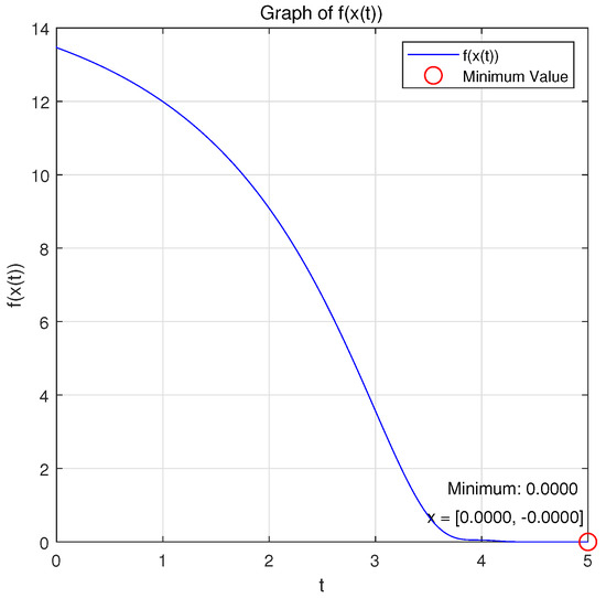
Figure 2.
Change in with respect to t.

Figure 3.
Change in with respect to .

Figure 4.
Change in with respect to .
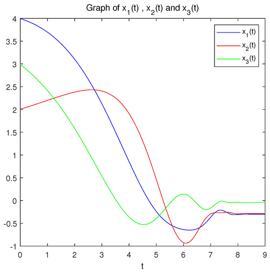
Figure 5.
Change in with respect to t.
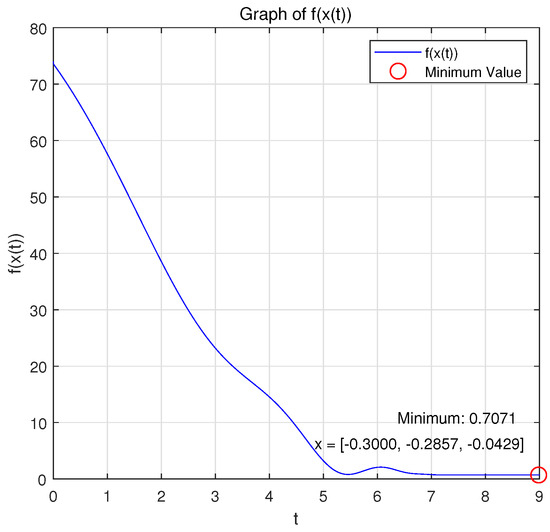
Figure 6.
Change in with respect to t.
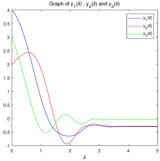
Figure 7.
Change in with respect to .
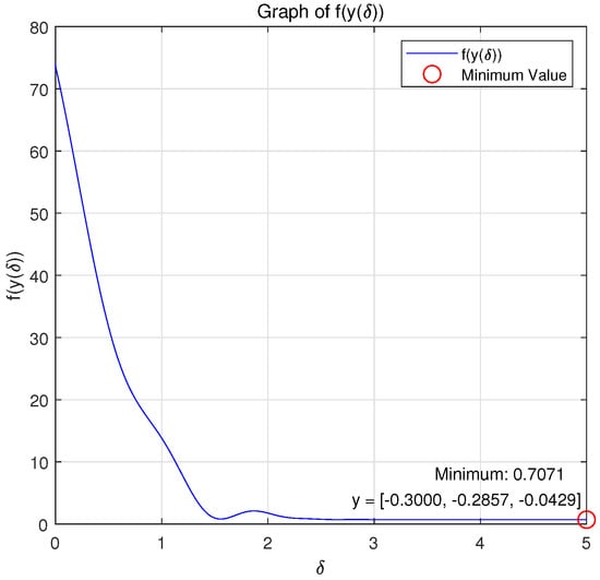
Figure 8.
Change in with respect to .
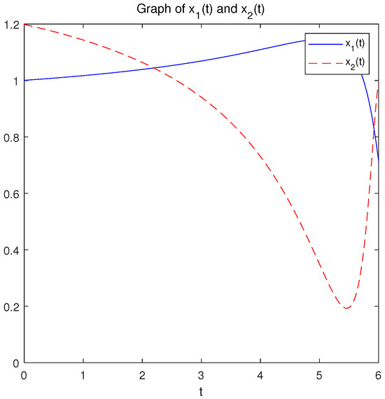
Figure 9.
Change in with respect to t.
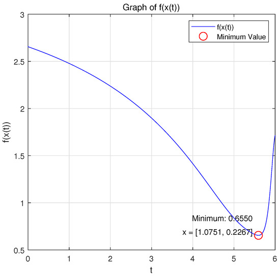
Figure 10.
Change in with respect to t.
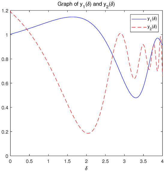
Figure 11.
Change in with respect to .
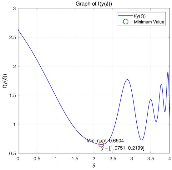
Figure 12.
Change in with respect to .
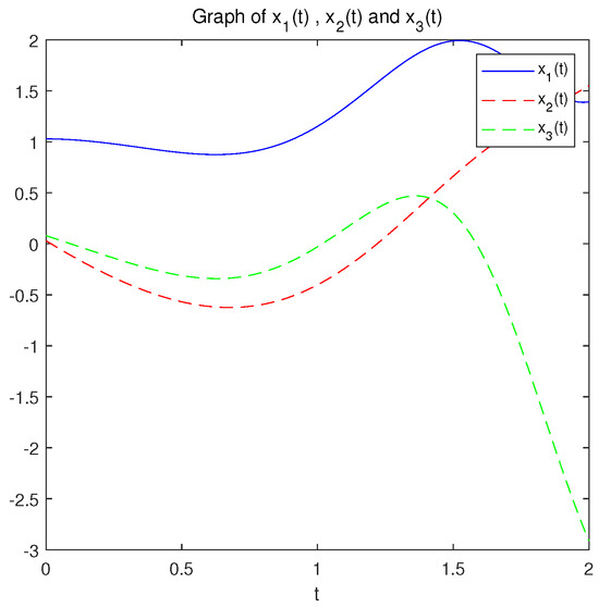
Figure 13.
Change in with respect to t.
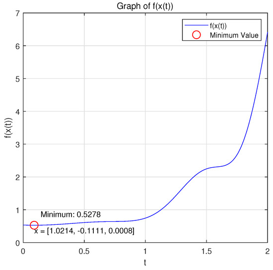
Figure 14.
Change in with respect to t.
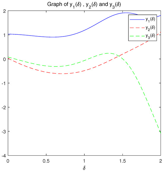
Figure 15.
Change in with respect to .
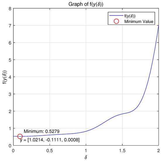
Figure 16.
Change in with respect to .
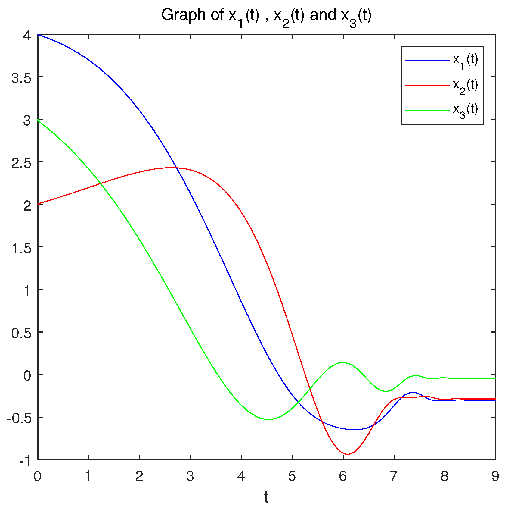
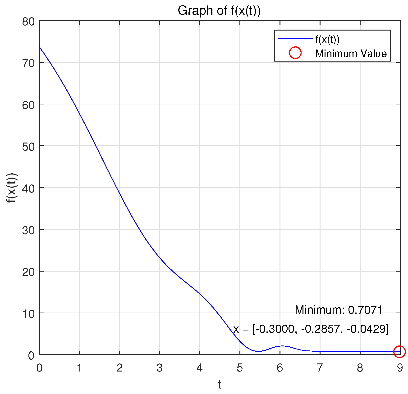
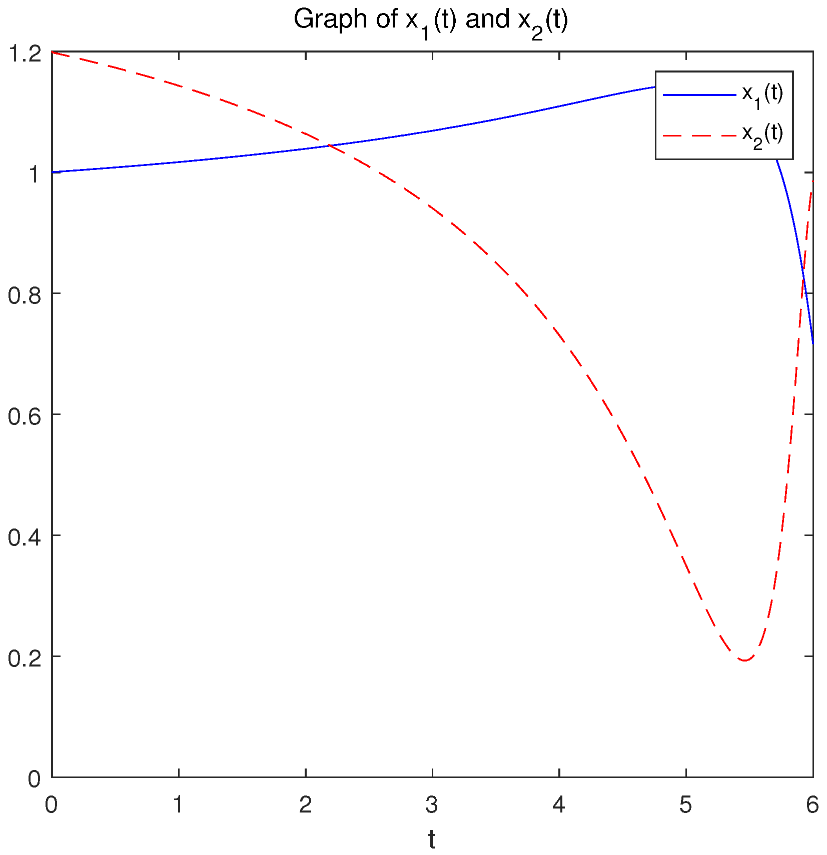
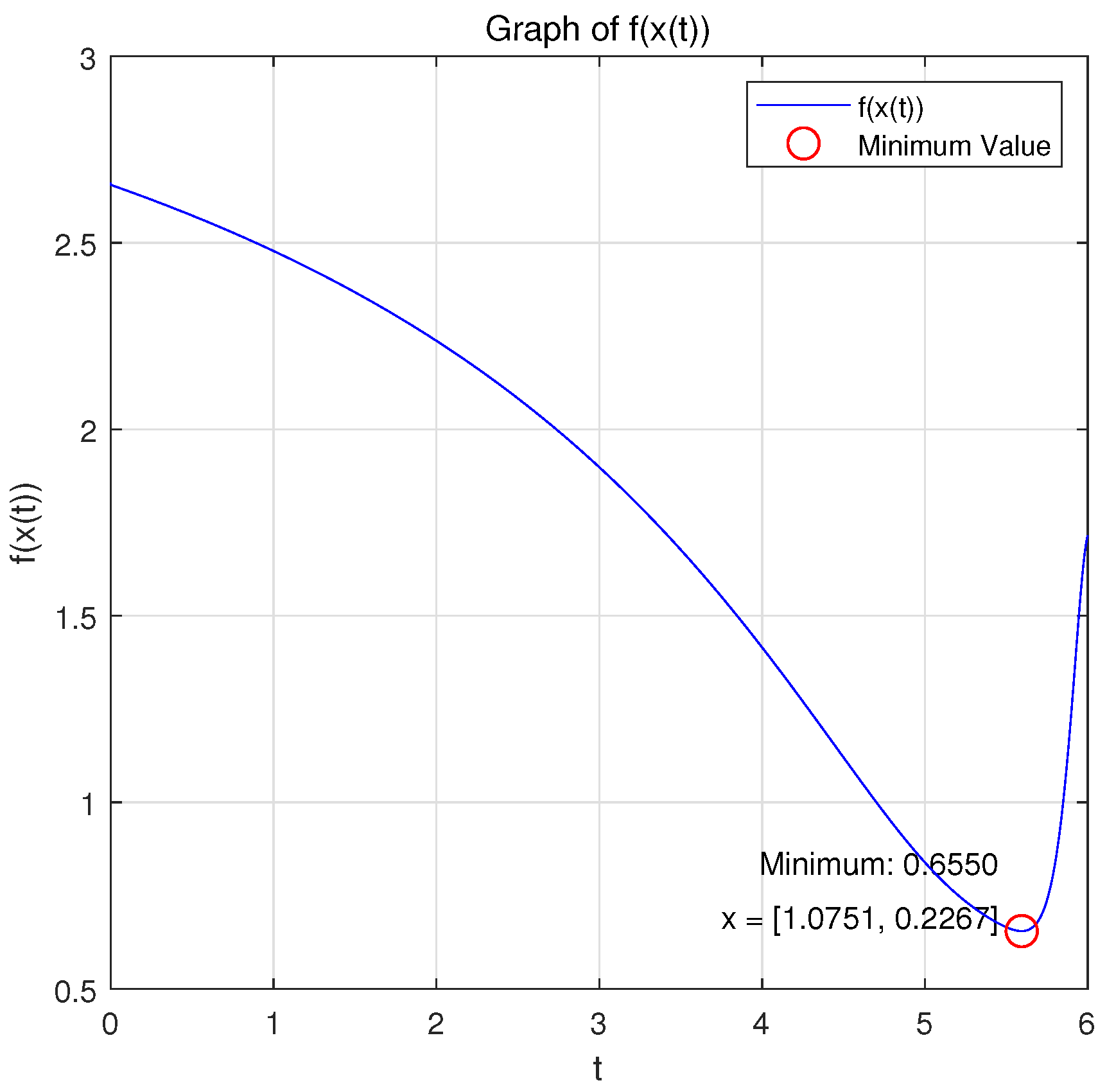
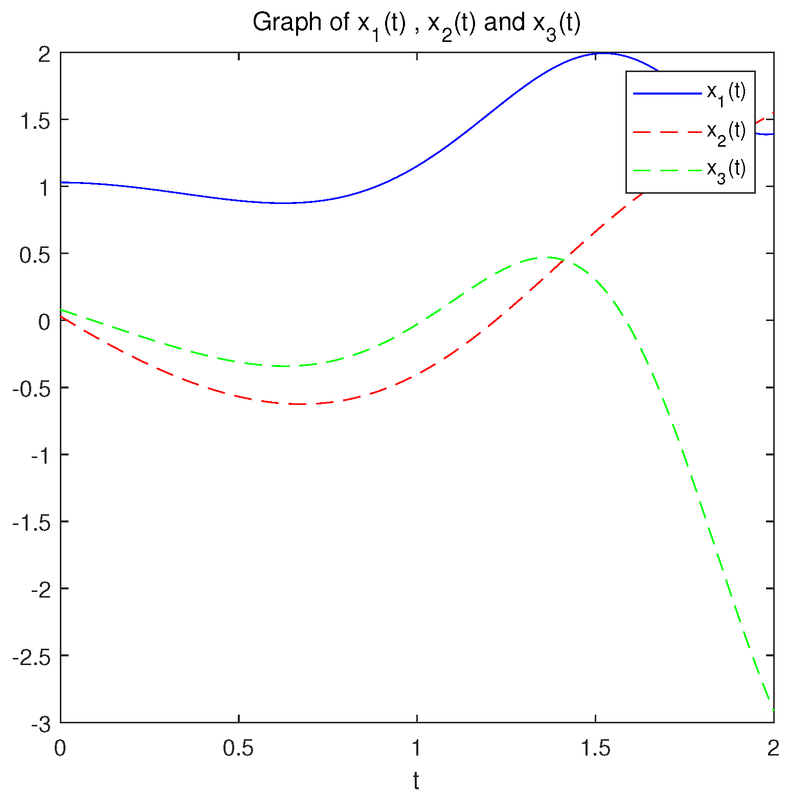
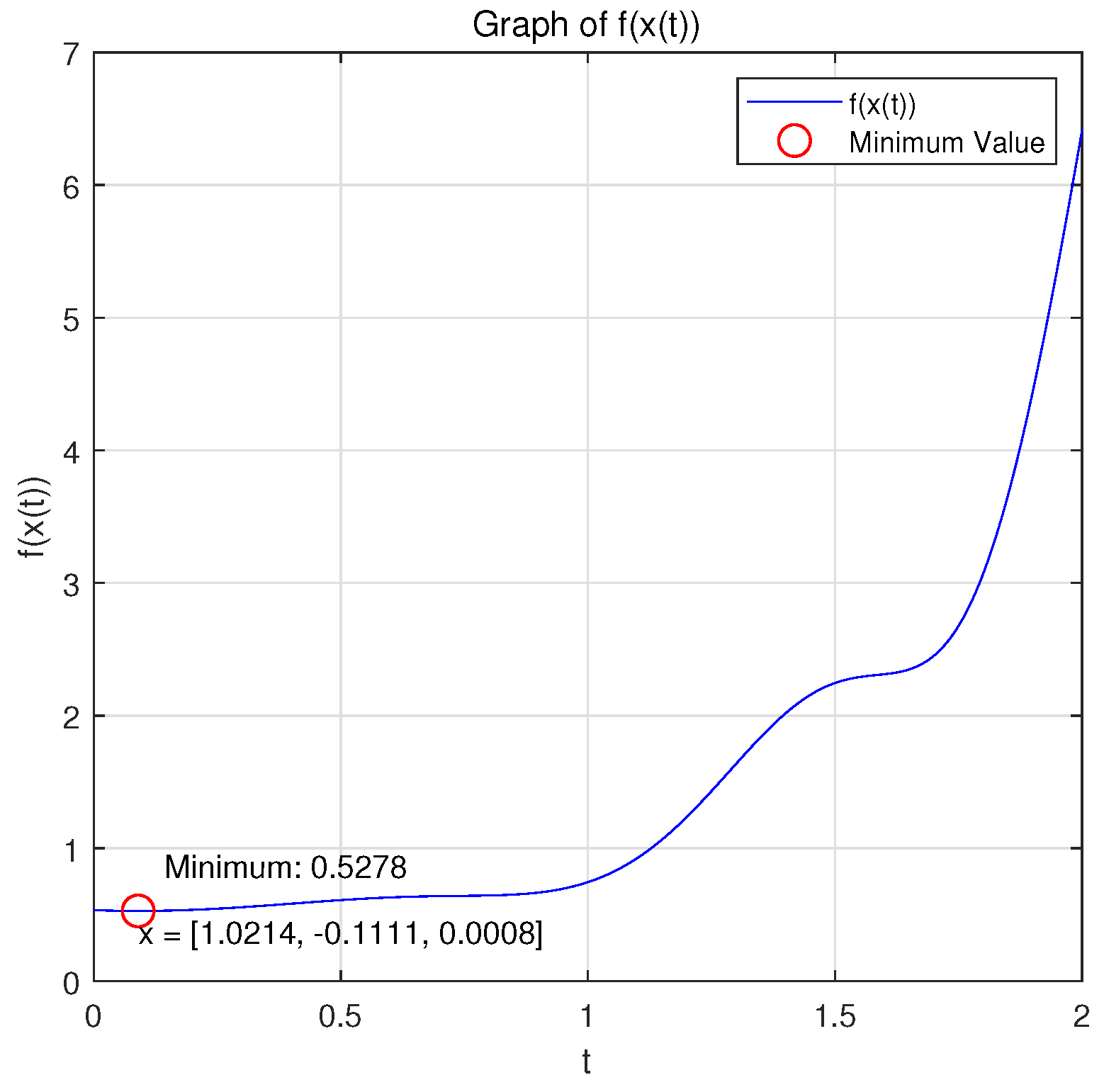
Case 3: When = 0.5, a = 2, = 1, T = 6, and A = , we choose and , and we consider the minimum of the strongly convex function .
Figure 1 and Figure 2 show the variations in the variables x and with respect to t when system (9a,b) was applied to solve the problem.
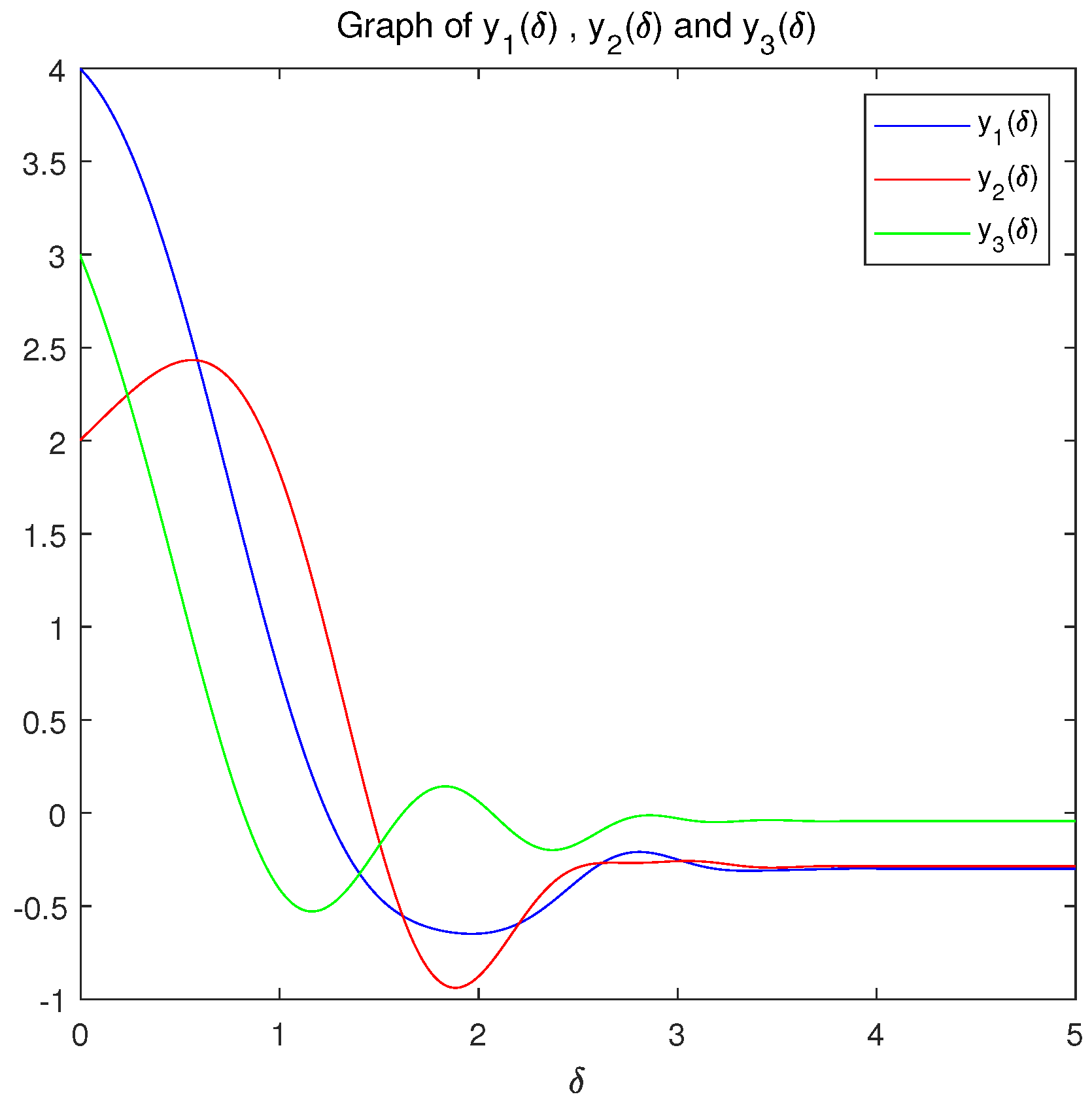
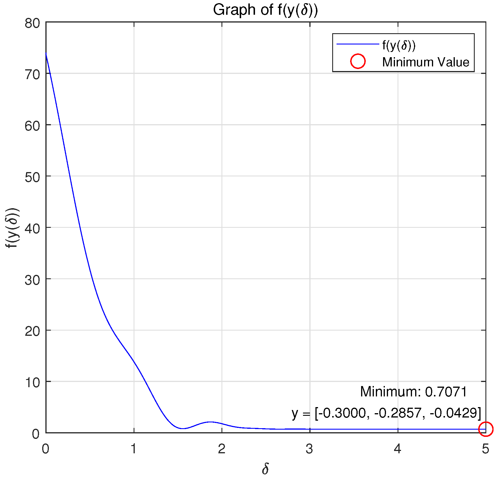
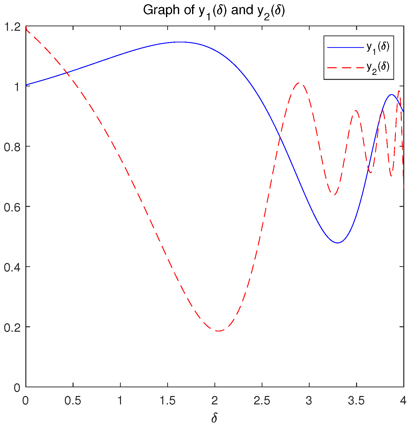
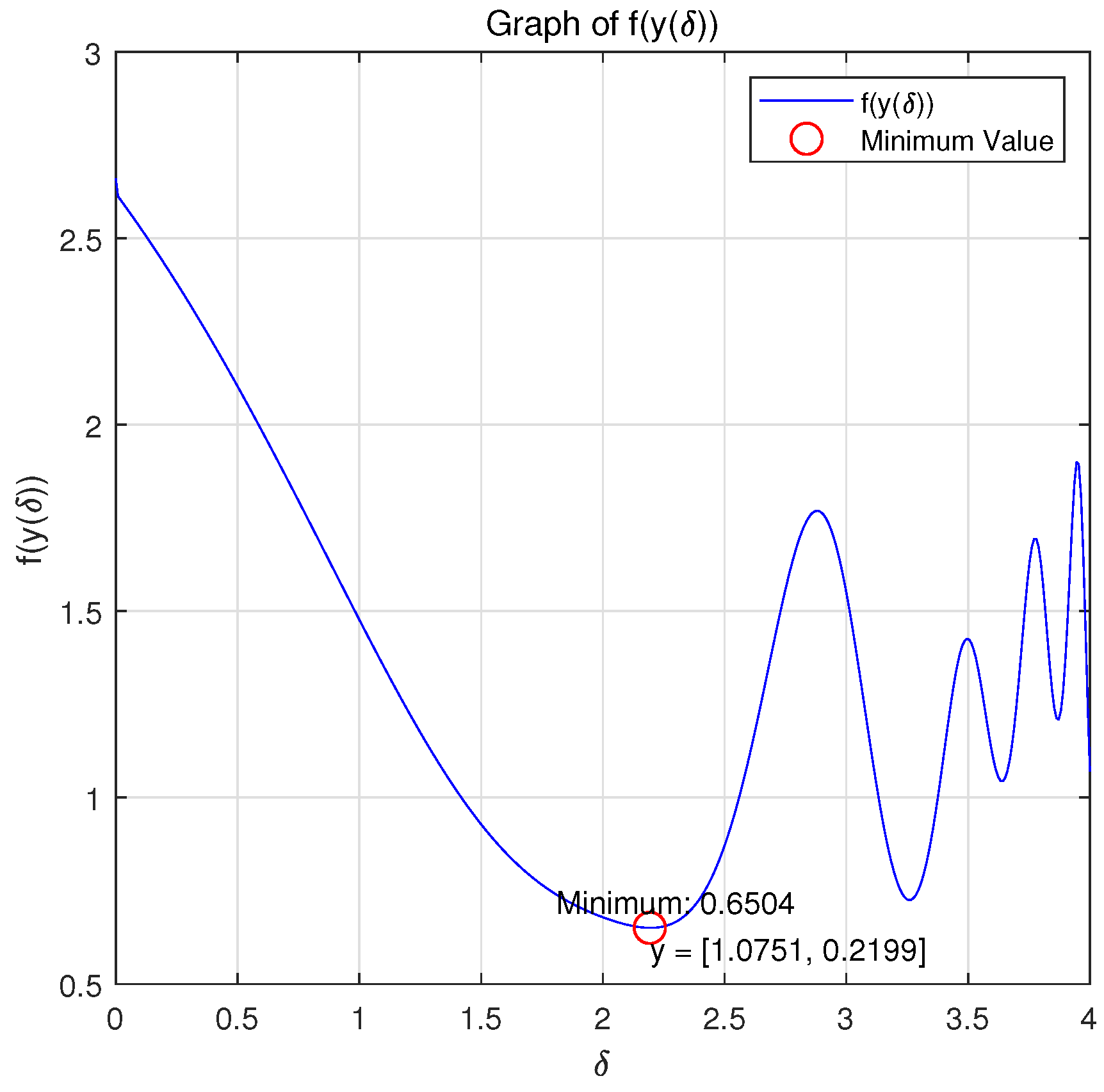
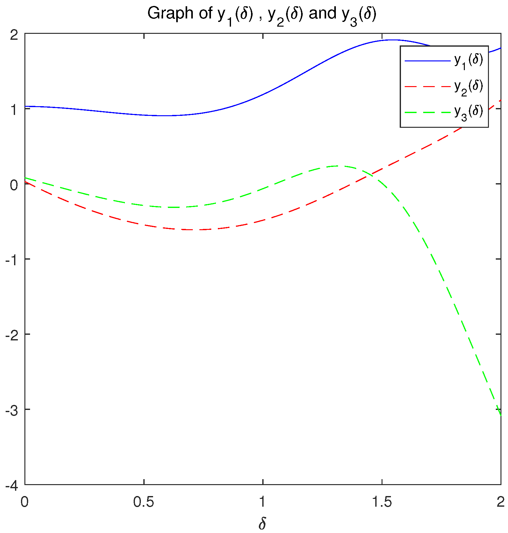
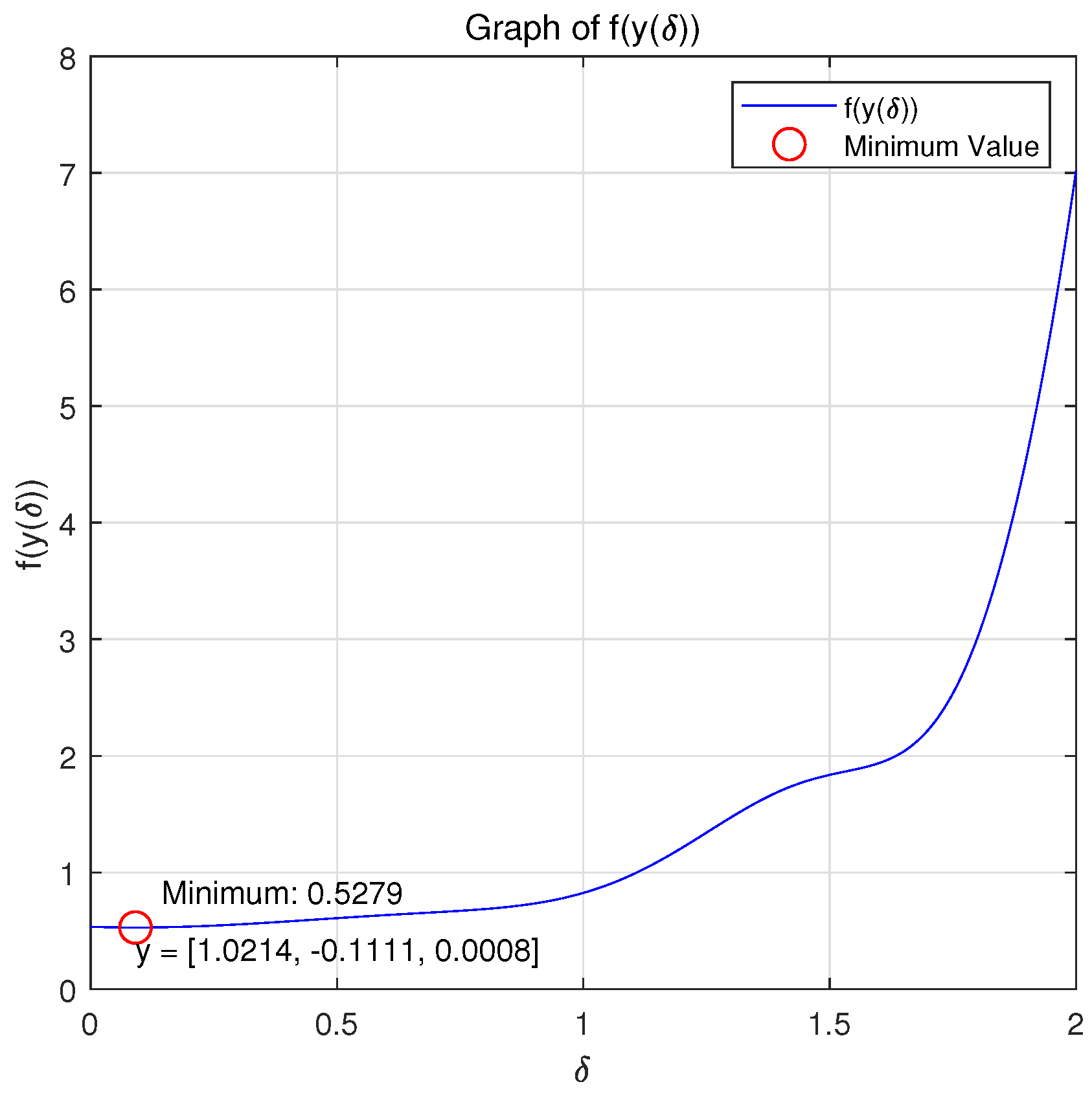
Figure 3 and Figure 4 show the variations in the variables y and f(y()) with respect to when system (14a,b) was applied to solve the problem.
Remark 5.
The optimization problem reached the optimal solution within the prescribed time under the action of system (9a,b), and the equivalent optimization problem converged asymptotically to the same optimal solution under the action of system (14a,b).
Case 4: When = 1, a = 3, T = 9.5, A = , c = , d = 1, and b = 1/2, we choose and , and we consider the minimum of the strongly convex function .
Figure 5 and Figure 6 show the variations in the variables x and with respect to t when system (9a,b) was applied to solve the problem.
Figure 7 and Figure 8 show the variations in the variables y and with respect to when system (14a,b) was applied to solve the problem.
Remark 6.
The optimization problem reached the optimal solution within the prescribed time under the action of system (9a,b), and the equivalent optimization problem converged asymptotically to the same optimal solution under the action of system (14a,b).
Case 5: When = 1, a = 0.5, T = 6.5, k = 0.9, A = , and b = , we choose and , and we consider the minimum of the strongly convex function .
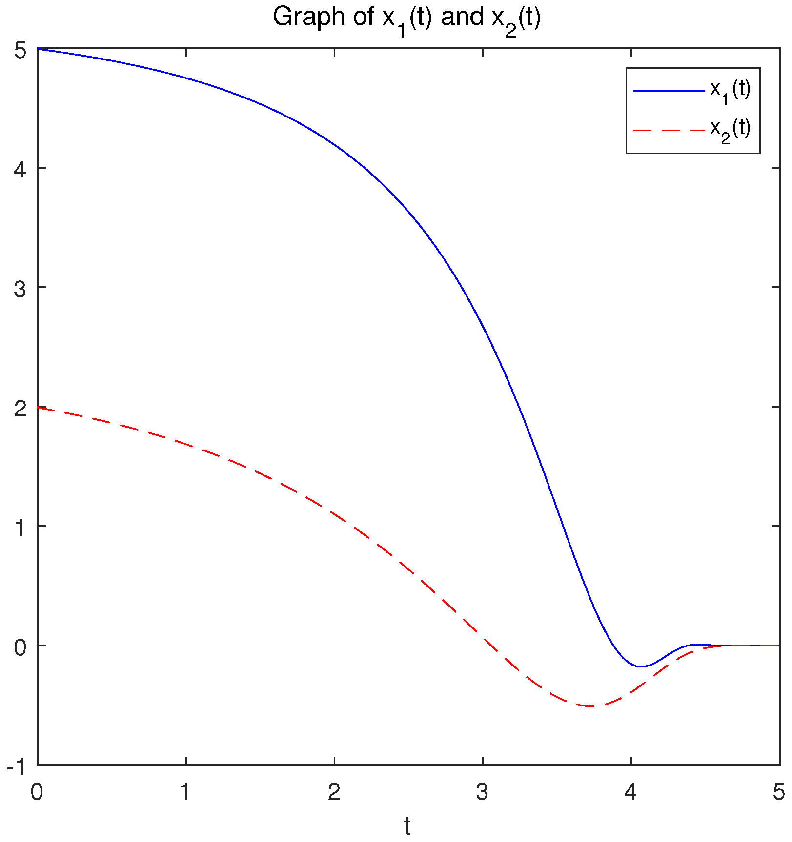
Figure 9 and Figure 10 show the variations in the variables x and with respect to t when system (17a,b) was applied to solve the problem.
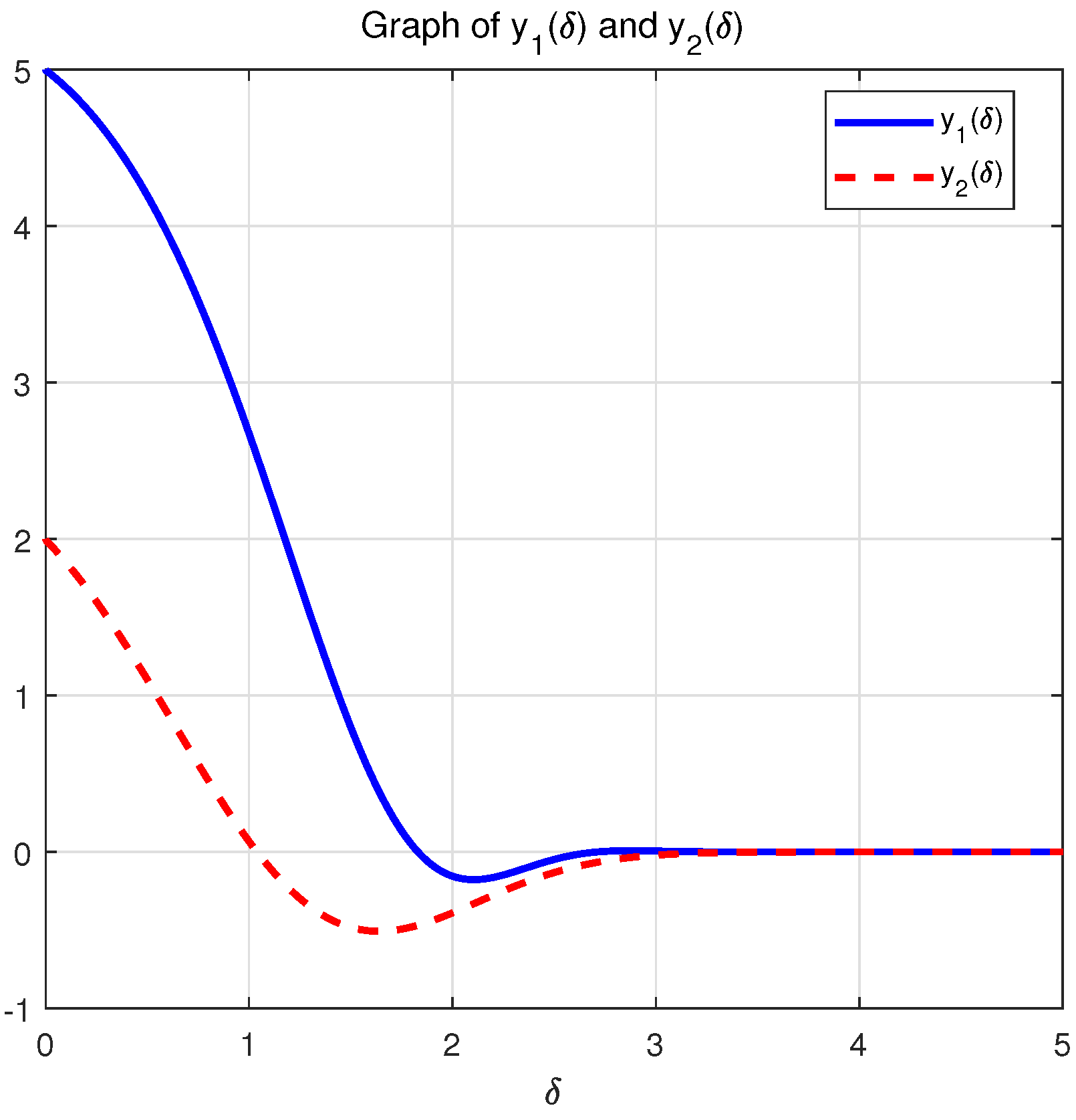
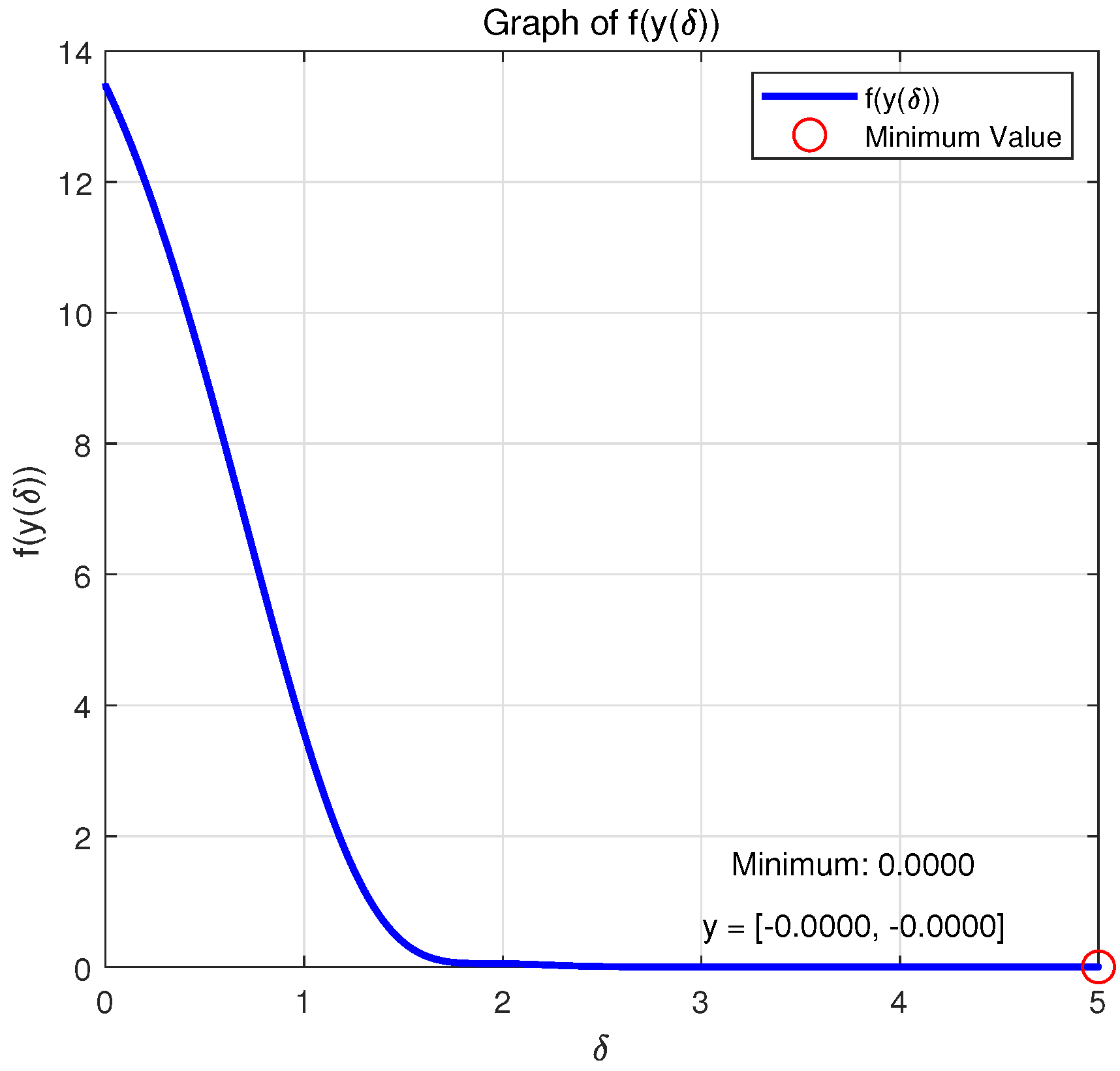
Figure 11 and Figure 12 show the variations in the variables y and with respect to when system (20a,b) was applied to solve the problem.
Remark 7.
Within the allowable error range, the optimization problem reached the optimal solution within the prescribed time under the action of system (17a,b), and the equivalent optimization problem converged asymptotically to the same optimal solution under the action of system (20a,b).
Case 6: When = 0.35, a = 0.8, T = 8, A = , and b = we choose and , and we consider the minimum of the strongly convex function .
Figure 13 and Figure 14 show the variations in the variables x and with respect to t when system (17a,b) was applied to solve the problem.
Figure 15 and Figure 16 show the variations in the variables y and with respect to when system (20a,b) was applied to solve the problem.
Remark 8.
The optimization problem reached the optimal solution within the prescribed time under the action of system (17a,b), and the equivalent optimization problem converged asymptotically to the same optimal solution under the action of system (20a,b).
7. Conclusions and Future Work
For the unconstrained optimization problem with a strongly convex objective function and the optimization problem with equality constraints, we develop a novel prescribed-time convergence acceleration algorithm with time rescaling. Our basic idea is to construct different second-order systems under certain conditions so that the two types of optimization problems converge to the optimal solution within the prescribed time T. These systems are more flexible than traditional exponential asymptotic convergence and significantly improve the convergence of the algorithm.
The advantage of our model is that it transforms the time t into an integral of (), i.e., . In this way, the second-order system we construct becomes more flexible, and convergence is achieved within the prescribed time T. The limitation of this paper is that our algorithm is only applicable to strongly convex functions, which limits its applicability to general convex and quasi-convex functions. Our future work will focus on the following:
(1) We will investigate the convergence of optimization problems with general convex and quasi-convex objective functions within the prescribed time T under the constraints of general convex sets or inequalities.
(2) In addition to the Euler method, we also hope to use the Runge–Kutta method and other methods to discretize the system and ensure that it converges to the optimal solution within the prescribed time T.
(3) We will explore acceleration algorithms for distributed optimization problems that converge within the prescribed time T.
Author Contributions
X.M.: Conceptualization, Funding acquisition, Methodology, Validation, Formal analysis, Writing—original draft. P.Z.: Supervision, Validation. H.J.: Writing—review & editing. Z.Y.: Sofware, Validation. All authors have read and agreed to the published version of the manuscript.
Funding
This research was supported by the National Natural Science Foundation of China (62163035), Technology Development Guided by the Central Government (ZYYD2022A05), the Tianshan Talent Training Program (2022TSYCLJ0004), the Ministry of Science and Technology Base and Talent Special Project—Third Xinjiang Scientific Expedition Project (2021xjkk1404), and Natural Science Foundation of Xinjiang Uygur Autonomous Region (grant No. 2022D01C45).
Data Availability Statement
No new data were created or analyzed in this study. Data sharing is not applicable to this article.
Conflicts of Interest
The authors declare no conflicts of interest. The funders had no role in the design of the study; in the collection, analyses, or interpretation of data; in the writing of the manuscript; or in the decision to publish the results.
References
- Polyak, B. Some methods of speeding up the convergence of iteration methods. USSR Comput. Math. Math. Phys. 1964, 4, 1–17. [Google Scholar] [CrossRef]
- Nesterov, Y.E. A method of solving a convex programming problem with convergence rate O(1/k2). Proc. USSR Acad. Sci. 1983, 269, 543–547. [Google Scholar]
- Nesterov, Y.E. One class of methods of unconditional minimization of a convex function, having a high rate of convergence. USSR Comput. Math. Math. Phys. 1985, 24, 80–82. [Google Scholar] [CrossRef]
- Nesterov, Y.E. An approach to the construction of optimal methods for minimization of smooth convex function. Èkonom. Mat. Metody 1988, 24, 509–517. [Google Scholar]
- Pierro, A.; Lopes, J. Accelerating iterative algorithms for symmetric linear complementarity problems. Int. J. Comput. Math. 1994, 50, 35–44. [Google Scholar] [CrossRef]
- Arihiro, K.; Satoshi, F.; Tadashi Ae Members. Acceleration by prediction for error back-propagation algorithm of neural network. Syst. Comput. Jpn. 1994, 25, 78–87. [Google Scholar]
- Beck, A.; Teboulle, M. A fast iterative shrinkage-thresholding algorithm for linear inverse problems. SIAM J. Imaging Sci. 2009, 2, 183–202. [Google Scholar] [CrossRef]
- Nesterov, Y.E. Gradient Methods for Minimizing Composite Objective Function; Technical Report Discussion Paper, 2007/76; Center for Operations Research and Econometrics (CORE): Leuven, Belgium, 2007. [Google Scholar]
- O’Donoghue, B.; Cand, E. Adaptive restart for accelerated gradient schemes. Found. Comput. Math. 2015, 15, 715–732. [Google Scholar] [CrossRef]
- Nguyen, N.C.; Fernandez, P.; Freund, R.M.; Peraire, J. Accelerated residual methods for the iterative solution of systems of equations. SIAM J. Sci. Comput. 2018, 40, A3157–A3179. [Google Scholar] [CrossRef]
- Song, Y.; Wang, Y.; Holloway, J.; Krstic, M. Time-varying feedback for regulation of normal-form nonlinear systems in prescribed finite time. Automatica 2017, 83, 243–251. [Google Scholar] [CrossRef]
- Li, H.; Zhang, M.; Yin, Z.; Zhao, Q.; Xi, J.; Zheng, Y. Prescribed-time distributed optimization problem with constraints. ISA Trans. 2024, 148, 255–263. [Google Scholar] [CrossRef] [PubMed]
- Liu, L.; Liu, P.; Teng, Z.; Zhang, L.; Fang, Y. Predefined-time position tracking optimization control with prescribed performance of the induction motor based on observers. ISA Trans. 2024, 147, 187–201. [Google Scholar] [CrossRef] [PubMed]
- Zhang, Y.; Chadli, M.; Xiang, Z. Prescribed-Time Adaptive Fuzzy Optimal Control for Nonlinear Systems. IEEE Trans. Fuzzy Syst. 2024, 32, 2403–2412. [Google Scholar] [CrossRef]
- Attouch, H.; Chbani, Z.; Riahi, H. Fast proximal methods via time scaling of damped inertial dynamics. SIAM J. Optim. 2019, 29, 2227–2256. [Google Scholar] [CrossRef]
- Attouch, H.; Chbani, Z.; Riahi, H. Fast convex optimization via time scaling of damped inertial gradient dynamics. Pure Appl. Funct. Anal. 2021, 6, 1081–1117. [Google Scholar]
- Attouch, H.; Chbani, Z.; Fadili, J.; Riahi, H. First-order optimization algorithms via inertial systems with Hessian driven damping. Math. Program. 2022, 193, 113–155. [Google Scholar] [CrossRef]
- Attouch, H.; Chbani, Z.; Fadili, J.; Riahi, H. Fast convergence of dynamical ADMM via time scaling of damped inertial dynamics. J. Optim. Theory Appl. 2022, 193, 704–736. [Google Scholar] [CrossRef]
- He, X.; Hu, R.; Fang, Y.P. Inertial primal-dual dynamics with damping and scaling for linearly constrained convex optimization problems. Appl. Anal. 2022, 102, 4114–4139. [Google Scholar] [CrossRef]
- Balhag, A.; Chbani, Z.; Attouch, H. Fast convex optimization via inertial dynamics combining viscous and Hessian-driven damping with time rescaling. Evol. Equ. Control Theory 2022, 11, 487–514. [Google Scholar]
- Hulett, D.A.; Nguyen, D.-K. Time Rescaling of a Primal-Dual Dynamical System with Asymptotically Vanishing Damping. Appl. Math. Optim. 2023, 88, 27. [Google Scholar] [CrossRef]
- Luo, H. A primal-dual flow for affine constrained convex optimization. ESAIM Control. Calc. Var. 2022, 28, 1–34. [Google Scholar] [CrossRef]
- Luo, H.; Chen, L. From differential equation solvers to accelerated first-order methods for convex optimization. Math. Program. 2021, 195, 735–781. [Google Scholar] [CrossRef]
- Chen, L.; Luo, H. A unified convergence analysis of first order convex optimization methods via strong lyapunov functions. arXiv 2021, arXiv:2108.00132. [Google Scholar]
- Luo, H. Accelerated primal-dual methods for linearly constrained convex optimization problems. arXiv 2021, arXiv:2109.12604v2. [Google Scholar]
- Tran, D.; Yucelen, T. Finite-time control of perturbed dynamical systems based on a generalized time transformation approach. Syst. Control Lett. 2020, 136, 104605. [Google Scholar] [CrossRef]

Disclaimer/Publisher’s Note: The statements, opinions and data contained in all publications are solely those of the individual author(s) and contributor(s) and not of MDPI and/or the editor(s). MDPI and/or the editor(s) disclaim responsibility for any injury to people or property resulting from any ideas, methods, instructions or products referred to in the content. |
© 2025 by the authors. Licensee MDPI, Basel, Switzerland. This article is an open access article distributed under the terms and conditions of the Creative Commons Attribution (CC BY) license (https://creativecommons.org/licenses/by/4.0/).