Bounded Rational Decision-Risk Propagation Coupling Dynamics in Directed Weighted Multilayer Hypernetworks

Abstract

Industrial symbiosis network (ISN) is crucial to improving resource utilization efficiency and promoting sustainable development. In order to mitigate the damage caused to symbiotic systems by risk propagation, this paper constructs a directed weighted multilayer hypernetwork model that considers bounded rational decision and risk propagation coupling ($\mathrm{U}{\mathrm{A}}^{\mathrm{P}}{\mathrm{A}}^{\mathrm{H}}\mathrm{U}-\mathrm{S}\mathrm{I}\mathrm{S}$), providing a new method for risk management in industrial symbiosis networks. This paper constructs a weighted hypernetwork model to simulate the interaction of risk information in a symbiotic network and uses a time-varying adaptive propagation mechanism to describe the changes in bounded rational decisions made by enterprises during the risk information interaction process. A directed weighted network is developed to simulate the evolution process of an industrial symbiosis network, with the network topology representing the risk propagation path. The study also considers the roles of mass media and crowd effects and innovatively introduces the assumption of decision incubation periods. The proposed coupled dynamic model is theoretically analyzed and numerically simulated by using the Microscopic Markov Chain Approach (MMCA). The findings indicate that enhancing the enterprises’ risk response willingness and risk perception ability, improving the risk recovery ability, and cooperating with timely and accurate media reports can effectively inhibit the risk propagation on ISN.

1. Introduction

Industrial symbiosis (IS) enables traditionally separate entities and companies to share and cooperate in materials, energy, and information [1], which contributes to improving sustainability [2,3] and brings environmental, economic, and social benefits [4,5]. The exchange of substances between symbiotic companies forms a dynamic and complex network known as the industrial symbiosis network (ISN).

As core nodes within industrial symbiotic networks, the stability of enterprises underpins the robust operation of the entire system. However, enterprises may encounter imbalances between the resource supply and the demand due to external environmental shifts or internal organizational coordination failures. This not only impacts their own production and operations but also transmits risks to partners through symbiotic linkages, ultimately posing significant risks to the entire industrial symbiotic system. The 2021 grounding of the Ever Given in the Suez Canal caused severe congestion and delays across global shipping networks, plunging numerous enterprises into supply chain disruptions and ultimately inflicting substantial economic losses upon multiple sectors, including automotive, retail, and electronics worldwide [6]. In 2017, Kobe Steel’s data falsification scandal triggered a global crisis of trust and safety concerns, severely undermining the credibility and reliability of the entire symbiotic network. Consequently, the stability of industrial symbiosis networks plays a vital role in societal production and economic development [7,8]. Investigating the patterns of risk propagation within industrial symbiosis networks thus holds significant theoretical and practical importance.

Implementing targeted risk management strategies to curb the propagation of risks is of significant importance. When enterprises come into contact with risk-related information through internal company systems, supply chain management systems, or industry information platforms, they are constrained by factors such as information asymmetry, resource limitations (risk management cost constraints), and cognitive biases, leading them to make ‘satisfactory solutions’ under bounded rationality rather than fully rational optimal solutions [9,10]. This paper draws on Herbert Simon’s adaptive strategy for simplifying decision dimensions [11], reducing complex and continuous risk attitudes to a binary ‘Hesitant-Positive’ typology. As an important carrier of risk information, mass media has a systematic impact on the bounded rational decision process of enterprises [12,13]. The timely and accurate nature of media reports will affect the decisions made by enterprises regarding risks. When media reports are timely and accurate, enterprises can establish effective risk warning mechanisms to prevent risks. Therefore, analyzing the bounded rational decision made by enterprises in the face of risks and the role of media reports in decision-making will help to more accurately describe the risk transmission mechanism in industrial symbiosis networks.

From a macro perspective, risk propagation in the industrial symbiosis network is considered a complex, network-driven phenomenon, which makes the complex network theory an effective tool for studying industrial risk propagation. Li et al. [14] applied the complex network theory to analyze the topological characteristics of symbiotic networks. Wang et al. [15] established a directed weighted network cascade failure model, demonstrating that the interaction between economic fluctuations and network structure is a key determinant of industrial symbiosis network vulnerability. Wu et al. [16] quantified environmental risks within steel industry symbiotic networks, providing evidence-based foundations for environmental risk mitigation strategies in industrial symbiosis networks. Shan et al. [17] developed multi-network frameworks to investigate the impact of risk information disclosure on risk propagation, subsequently exploring the influence of risk sharing on risk transmission within multi-path networks [18]. However, given the intricate information-sharing mechanisms among enterprises within industrial symbiosis networks, simple peer-to-peer information propagation models are no longer adequate. Within hypernetworks, risk information can propagate simultaneously across multiple symbiotic enterprises via hyperedges, more accurately reflecting real-world information flows [19,20]. Therefore, this paper constructs a directed weighted multilayer hypernetwork model that accounts for bounded rationality decision-making and risk propagation coupling, offering a novel approach to risk management within industrial symbiosis networks.

The main contributions of this paper are as follows:

• This paper employs weighted hypernetwork models to simulate risk information interaction in symbiotic networks and uses a directed weighted network model to describe risk propagation among symbiotic enterprises, thereby forming a directed weighted multilayer hypernetwork model that considers bounded rational decision and risk propagation coupling ($\mathrm{U}{\mathrm{A}}^{\mathrm{P}}{\mathrm{A}}^{\mathrm{H}}\mathrm{U}-\mathrm{S}\mathrm{I}\mathrm{S}$);
• A time-varying adaptive communication mechanism is used to describe changes in bounded rational decisions made by enterprises during the risk information interaction process, while introducing the influence of mass media and crowd effects. During the risk propagation process the influence of the degree of symbiotic dependence between enterprises and the k-shell value of enterprises on risk propagation is considered, and the assumption of a decision incubation period is innovatively introduced;
• The Microscopic Markov Chain Approach (MMCA) is used to perform theoretical analysis and numerical simulation of the proposed coupled dynamic model.

The rest of this paper is structured as follows. Section 2 introduces the construction process of the directed weighted multilayer hypernetwork model and the coupling mechanism of bounded rational decision and risk propagation. In Section 3, the dynamic equations satisfied by the hyperdegree of nodes in the weighted hypernetworks are calculated, and the proposed coupled dynamic model is theoretically analyzed using the Microscopic Markov Chain Approach (MMCA). Section 4 conducts numerical simulation verification of the theoretical derivations in Section 3. Based on the numerical simulation results in Section 4, Section 5 provides relevant risk management recommendations.

2. Model Description

The Kalundborg Symbiosis in Denmark is one of the world’s most famous and successful examples of industrial symbiosis [7,21,22]. The symbiosis began in the 1960s when a small number of companies (such as the Asnæs Power Station, the Statoil refinery, and the Gypsum Plasterboard Factory) spontaneously launched a resource exchange cooperation based on economic and environmental benefits. Over time, more companies (such as Novo Nordisk Pharmaceuticals and soil remediation companies) and municipal departments gradually joined in, forming a complex industrial symbiosis network through multi-level recycling of resources and by-products. In this process, cooperation among various entities gradually expanded from bilateral transactions to multilateral collaboration, ultimately propelling Kalundborg to become a global model for industrial ecologization.

This paper employs a weighted hypernetwork model to simulate risk information interaction among symbiotic enterprises and constructs a directed weighted network model that considers the relationship between resource supply and demand to generate an industrial symbiosis network. The topological structure of the network is shown in Figure 1, where the nodes in each layer are the same, but each layer exhibits different evolutionary processes and topological structures.

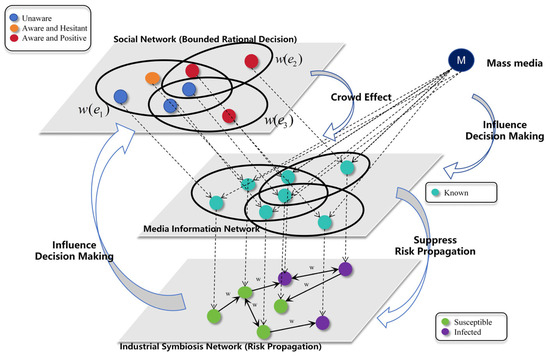
Figure 1. Schematic diagram of the directed weighted multilayer hypernetwork model. Node M represents the Mass media, which is connected to every node in the network and influences the bounded rational decision-making process. The top layer corresponds to the transmission of risk information on social networks. There are three types of bounded rational decisions made by enterprises: unaware ($\mathrm{U}$), aware and hesitant (${\mathrm{A}}^{\mathrm{H}}$), and aware and positive (${\mathrm{A}}^{\mathrm{P}}$). The middle layer represents that each node can obtain risk information from mass media reports, and each node is known ($\mathrm{K}$). The bottom layer represents the risk propagation layer, where nodes have two states: susceptible ($\mathrm{S}$) and infected ($\mathrm{I}$).

Next, this section first introduces the basic concepts involved in the directed weighted multilayer hypernetwork model, then describes the evolution mechanism of the network model, and finally proposes the coupling dynamics rules.

2.1. Related Concepts

2.1.1. Hypernetworks Based on Hypergraphs

Let $\mathrm{V}=\left\{{\mathrm{v}}_1,{\mathrm{v}}_2,\dots ,{\mathrm{v}}_{\mathrm{n}}\right\}$ be a non-empty and finite set, and let ${\mathrm{e}}_{\mathrm{i}}=\left\{{\mathrm{v}}_{\mathrm{i}1},{\mathrm{v}}_{\mathrm{i}2},\dots ,{\mathrm{v}}_{\mathrm{i}\mathrm{j}}\right\}$, ${\mathrm{v}}_{\mathrm{i}\mathrm{k}}\in \mathrm{V},\mathrm{k}=\mathrm{1,2},\dots ,\mathrm{j}$, and $\mathrm{E}=\left\{{\mathrm{e}}_1,{\mathrm{e}}_2,\dots ,{\mathrm{e}}_{\mathrm{m}}\right\}$ be a family of subsets of $\mathrm{V}$. The pair $\mathrm{H}=\left(\mathrm{V},\mathrm{E}\right)$ is called a hypergraph, where the elements ${\mathrm{v}}_1,{\mathrm{v}}_2,\dots ,{\mathrm{v}}_{\mathrm{n}}$ of $\mathrm{V}$ are called the nodes or vertices and ${\mathrm{e}}_{\mathrm{i}}\left(\mathrm{i}=\mathrm{1,2},\dots ,\mathrm{m}\right)$ are called the hyperedges. The triple $\mathrm{H}=\left(\mathrm{V},\mathrm{E},\mathrm{W}\right)$ is called a weighted hypergraph, where $\mathrm{V}=\left\{{\mathrm{v}}_1,{\mathrm{v}}_2,\dots ,{\mathrm{v}}_{\mathrm{n}}\right\}$, $\mathrm{E}=\left\{{\mathrm{e}}_1,{\mathrm{e}}_2,\dots ,{\mathrm{e}}_{\mathrm{m}}\right\}$, and $\mathrm{W}=\left\{{\mathrm{w}}_1,{\mathrm{w}}_2,\dots ,{\mathrm{w}}_{\mathrm{m}}\right\}$ are the sets of nodes, hyperedges, and weights, respectively. In hypergraph, if there exists a hyperedge that encompasses two nodes, the two nodes are said to be adjacent. Suppose that $\mathsf{\Omega }=\left(\mathrm{V},\mathrm{E},\mathrm{W}\right)$ is a finite weighted hypergraph and $\mathrm{G}$ is a map from $\mathrm{T}=\left[0,\mathrm{\infty }\right]$ into $\mathsf{\Omega }$. For any given $\mathrm{t}\ge 0$, $\mathrm{G}\left(\mathrm{t}\right)=\left(\mathrm{V}\left(\mathrm{t}\right),\mathrm{E}\left(\mathrm{t}\right),\mathrm{W}\left(\mathrm{t}\right)\right)$ is a finite weighted hypergraph. A weighted hypernetwork $\left\{\mathrm{G}\left(\mathrm{t}\right),\mathrm{t}\in \mathrm{T}\right\}$ is a collection of weighted hypergraphs [23]. The hyperdegree of node ${\mathrm{v}}_{\mathrm{j}}$ is defined as the number of hyperedges associated with that node, denoted as ${\mathrm{h}}_{\mathrm{j}}=\sum _{\mathrm{i}=1}^{\mathrm{m}}{\mathrm{c}}_{\mathrm{i}\mathrm{j}}$, where ${\mathrm{c}}_{\mathrm{i}\mathrm{j}}=\left\{\begin{array}{c}1 {\mathrm{v}}_{\mathrm{j}}\in {\mathrm{e}}_{\mathrm{i}}\\ 0 \mathrm{otherwise}\end{array}\right.$ is the element in the incidence matrix $\mathrm{C}={\left({\mathrm{c}}_{\mathrm{i}\mathrm{j}}\right)}_{\mathrm{m}\times \mathrm{n}}$.

2.1.2. Directed Weighted Network

• The weight matrix of the directed weighted network is defined as $\mathrm{W}={\left({\mathrm{w}}_{\mathrm{i}\mathrm{j}}\right)}_{\mathrm{n}\times \mathrm{n}}$, where ${\mathrm{w}}_{\mathrm{i}\mathrm{j}}\ge 0$. In this paper, ${\mathrm{w}}_{\mathrm{i}\mathrm{j}}$ represents the amount of resources provided by symbiotic enterprise ${\mathrm{v}}_{\mathrm{i}}$ to ${\mathrm{v}}_{\mathrm{j}}$;
• The degree of node ${\mathrm{v}}_{\mathrm{i}}$ is divided into in-degree (${\mathrm{k}}_{\mathrm{i}}^{\mathrm{i}\mathrm{n}}$) and out-degree (${\mathrm{k}}_{\mathrm{i}}^{\mathrm{o}\mathrm{u}\mathrm{t}}$). The degree of node ${\mathrm{v}}_{\mathrm{i}}$ is equal to the sum of its out-degree and in-degree (${{\mathrm{k}}_{\mathrm{i}}=\mathrm{k}}_{\mathrm{i}}^{\mathrm{i}\mathrm{n}}+{\mathrm{k}}_{\mathrm{i}}^{\mathrm{o}\mathrm{u}\mathrm{t}}$) [14]. In this paper, the degree of enterprise ${\mathrm{v}}_{\mathrm{i}}$ represents the number of enterprises that have a symbiotic relationship with it;
• The strength of a node is defined as the sum of the weights of the directed edges connected to that node [24,25]. The in-strength (${\mathrm{s}}_{\mathrm{i}}^{\mathrm{i}\mathrm{n}}$) and out-strength (${\mathrm{s}}_{\mathrm{i}}^{\mathrm{o}\mathrm{u}\mathrm{t}}$) of node ${\mathrm{v}}_{\mathrm{i}}$ are defined as the following Equation (1):

  $${\mathrm{s}}_{\mathrm{i}}^{\mathrm{i}\mathrm{n}}={\sum }_{\mathrm{j}\in {\mathsf{\Omega }}_{\mathrm{i}}^{\mathrm{i}\mathrm{n}}}{\mathrm{w}}_{\mathrm{j}\mathrm{i}}, {\mathrm{s}}_{\mathrm{i}}^{\mathrm{o}\mathrm{u}\mathrm{t}}={\sum }_{\mathrm{j}\in {\mathsf{\Omega }}_{\mathrm{i}}^{\mathrm{o}\mathrm{u}\mathrm{t}}}{\mathrm{w}}_{\mathrm{i}\mathrm{j}},$$

  (1)
  where ${\mathsf{\Omega }}_{\mathrm{i}}^{\mathrm{i}\mathrm{n}}$ and ${\mathsf{\Omega }}_{\mathrm{i}}^{\mathrm{o}\mathrm{u}\mathrm{t}}$ are the set of in-neighbors and out-neighbors of enterprise ${\mathrm{v}}_{\mathrm{i}}$, respectively. The strength of enterprise ${\mathrm{v}}_{\mathrm{i}}$ is equal to the sum of the out-strength and in-strength, that is ${{\mathrm{s}}_{\mathrm{i}}=\mathrm{s}}_{\mathrm{i}}^{\mathrm{i}\mathrm{n}}+{\mathrm{s}}_{\mathrm{i}}^{\mathrm{o}\mathrm{u}\mathrm{t}}$;
• Given that resource inflows and outflows may differ significantly between symbiotic firms, this paper defines the degree of symbiotic dependence in terms of two-way resource dependence, that is as follows:

  $${\eta }_{ij}={\displaystyle \frac{e^{-w_{ij}/2}{·w}_{ij}+e^{-w_{ji}/2}{·w}_{ji}}{e^{-w_{ij}/2}+e^{-w_{ji}/2}}}.$$

  (2)

2.1.3. Jaccard Similarity

Jaccard similarity is an effective similarity measurement method that has been widely applied in fields such as bioinformatics [26,27], machine learning [28,29], and complex networks [30,31]. In this paper, assuming that ${\mathsf{\Omega }}_{\mathrm{i}}$ and ${\mathsf{\Omega }}_{\mathrm{j}}$ represent the sets of neighbors of nodes ${\mathrm{v}}_{\mathrm{i}}$ and ${\mathrm{v}}_{\mathrm{j}}$ in a directed weighted network, respectively, the similarity between ${\mathrm{v}}_{\mathrm{i}}$ and ${\mathrm{v}}_{\mathrm{j}}$ is as defined below:

$$J\left(i,j\right)=J_{ij}={\displaystyle \frac{\left|{\Omega }_i\cap {\Omega }_j\right|}{\left|{\Omega }_i\cup {\Omega }_j\right|}}$$

(3)

2.1.4. K-Core

A k-shell is defined as a subgraph of a network in which the degree of each node is no less than $\mathrm{k}$. By repeatedly removing nodes with degrees less than $\mathrm{k}$, k-shell decomposition of the network can be obtained [32]. The k-shell value $\mathrm{k}\_\mathrm{s}$ of a node indicates its core position in the network, with higher values indicating a more central position [33,34].

2.2. Generation of the Directed Weighted Multilayer Hypernetworks

2.2.1. Generation of the Social Network

The emergence of numerous social media platforms has provided numerous channels for symbiotic enterprises to exchange information. The hyperedges of the hypernetwork contain an arbitrary number of nodes and can accurately describe the high-order interactivity between symbiotic enterprises. In the hypernetwork described in this paper, nodes represent enterprises, and hyperedges represent information interactions between enterprises. This paper assumes that the formation of hyperedges follows a hyperdegree priority connection mechanism [23]. The evolution process of the network can be summarized as the addition of new node batches, the generation of new hyperedges, and the reconnection of existing hyperedges. The steps for constructing the upper-level social network are as follows.

Figure 2 presents a schematic illustration of the social network construction process, while Table 1 provides a detailed enumeration of the definitions and values of the parameters necessary for constructing the social network.

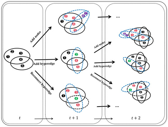
Figure 2. Schematic diagram of the hypernetwork construction process from time $\mathrm{t}$ to $\mathrm{t}+2$. The hypernetwork construction involves three operations: add nodes, add hyperedges, and reconnect hyperedges. Solid black lines represent existing hyperedges. Dashed black lines represent hyperedges removed during the reconnecting process. Dashed blue lines represent new hyperedges formed by newly added batches of nodes. Purple nodes represent the new node batches that have been added. The green nodes represent the nodes randomly selected when adding or reconnecting the hyperedge. The pink nodes represent the selected existing nodes.

Table 1. The definitions and values of the parameters necessary for constructing the social network.

Parameters	Descriptions	Value
${\mathrm{N}}_0$	The number of seed nodes	6
${\mathsf{\lambda }}^{\prime }$	The rate of new node batches arrivals	2
$\mathrm{f}\left(\mathrm{a}\right)$	Probability density function describing the distribution of the number of nodes per batch	U (4,6)
$\mathrm{g}\left(\mathrm{b}\right)$	Probability density function describing the distribution of the number of selected existing nodes	U (6,28)
${\mathrm{q}}_1$	Probability of adding new node batches	0.5
${\mathrm{q}}_2$	Probability of adding new hyperedges	0.2
${\mathrm{q}}_3$	Probability of reconnecting hyperedges	0.3
${\mathrm{m}}_1$	The number of new hyperedges formed in adding new node batches	U (7,12)
${\mathrm{m}}_2$	The number of new hyperedges formed in adding new hyperedges	U (6,8)
${\mathrm{m}}_3$	The number of reconnected hyperedges	U (7,9)

Step 1 Initialization. The initial hypernetwork is constituted by ${\mathrm{N}}_0$ seed nodes and a hyperedge containing them.

Step 2 Growth. At each time instant one of the following scenarios occurs with corresponding probability, where ${\mathrm{q}}_1+{\mathrm{q}}_2+{\mathrm{q}}_3=1$.

• New node batches are added with probability ${\mathrm{q}}_1$.
  Suppose that new node batches nodes arrive at the system according to a Poisson process $\mathrm{N}\left(\mathrm{t}\right)$ with rate ${\mathsf{\lambda }}^{\prime }$. When a new batch of ${\mathrm{a}}_{\mathrm{N}\left(\mathrm{t}\right)}$ nodes is added to the network at time t, these ${\mathrm{a}}_{\mathrm{N}\left(\mathrm{t}\right)}$ new nodes and ${\mathrm{b}}_{\mathrm{N}\left(\mathrm{t}\right)}$ previously existing nodes are encircled by a new hyperedge, totally ${\mathrm{m}}_1$ new hyperedges are constructed with no repetitive hyperedges. ${\mathrm{a}}_{\mathrm{N}\left(\mathrm{t}\right)}$ and ${\mathrm{b}}_{\mathrm{N}\left(\mathrm{t}\right)}$ are positive integers that are taken from the given probability density functions $\mathrm{f}\left(\mathrm{a}\right)$ and $\mathrm{g}\left(\mathrm{b}\right)$, respectively. ($\overline{\mathrm{a}}=\int \mathrm{a}\mathrm{f}\left(\mathrm{a}\right)\mathrm{d}\mathrm{a}<\mathrm{\infty }$, $\overline{\mathrm{b}}=\int \mathrm{b}\mathrm{g}\left(\mathrm{b}\right)\mathrm{d}\mathrm{b}<\mathrm{\infty }$). The selected probability ${\mathsf{\Pi }}_{\mathrm{j}}\left(\mathrm{t},{\mathrm{t}}_{\mathrm{i}}\right)$ for the $\mathrm{j}$ th node of the $\mathrm{i}$ th batch depends on the hyperdegree ${\mathrm{h}}_{\mathrm{j}}\left(\mathrm{t},{\mathrm{t}}_{\mathrm{i}}\right)$, that is,

  $${\mathsf{\Pi }}_{\mathrm{j}}\left(\mathrm{t},{\mathrm{t}}_{\mathrm{i}}\right)={\displaystyle \frac{{\mathrm{h}}_{\mathrm{j}}\left(\mathrm{t},{\mathrm{t}}_{\mathrm{i}}\right)}{\sum _{\mathrm{i},\mathrm{j}}{\mathrm{h}}_{\mathrm{j}}\left(\mathrm{t},{\mathrm{t}}_{\mathrm{i}}\right)}},$$

  (4)

  where ${\mathrm{t}}_{\mathrm{i}}$ denotes the time when the $\mathrm{i}$ th batch of nodes enters into the network.
• New hyperedges are added with probability ${\mathrm{q}}_2$.
  Randomly select a node in the network that is encircled by a new hyperedge along with ${\mathrm{b}}_{\mathrm{N}\left(\mathrm{t}\right)}$ existing nodes that are selected with the probability shown in Equation (3). Repeat this process until ${\mathrm{m}}_2$ new hyperedges without duplicates have been constructed.
• Existing hyperedges are reconnected with probability ${\mathrm{q}}_3$.
  Randomly select a node and a hyperedge containing it. The selected hyperedge is then disconnected, and the node is incorporated into a newly formed hyperedge with ${\mathrm{b}}_{\mathrm{N}\left(\mathrm{t}\right)}$ existing nodes that selected with the probability shown in Equation (3). Repeat this process until ${\mathrm{m}}_3$ new hyperedges without duplication are reconnected.

Step 3 Repeat. Repeat step 2 until the network size reaches the preset value.

2.2.2. Generation of the ISN

This paper uses the evolution mechanism of BBV [35] and the linear preferred connection mechanism of the BA model [36] to construct the ISN. The evolution process of a directed weighted network can be summarized as the addition of nodes, the formation of new directed edges, and the disconnection of existing directed edges. Table 2 lists the parameter definitions and their values required for this section. It is important to note that enterprises in the ISN are only able to generate new directed edges with existing nodes in the same hyperedge of the social network.

Table 2. The definitions and values of the parameters necessary for constructing the ISN.

Parameters	Descriptions	Value
${\mathrm{N}}_0$	The number of seed nodes	6
${\mathrm{w}}_0$	The initial weights	1
${\mathrm{q}}_1^{\prime }$	Probability of adding new nodes	0.5
${\mathrm{q}}_2^{\prime }$	Probability of adding new directed edges	0.3
${\mathrm{q}}_3^{\prime }$	Probability of disconnecting existing directed edges	0.2
${\mathrm{m}}_4$	The number of directed edges generated when adding a new node	8
${\mathrm{m}}_5$	The number of existing directed edges to disconnect	2
${\mathrm{p}}_1$	Probability of success of an event in a binomial distribution	0.5
$\mathsf{ϵ}$	The increase in weight when adding new nodes	3
$\mathsf{\sigma }$	The increase in weight when adding new directed edges	1

Step 1 Initialization. The initial network is a fully coupled network comprising ${\mathrm{N}}_0$ seed nodes and all initial weights set to ${\mathrm{w}}_0$.

Step 2 Growth. At each time instant, one of the following dynamic evolution rules is chosen, where ${\mathrm{q}}_1^{\prime }+{\mathrm{q}}_2^{\prime }+{\mathrm{q}}_3^{\prime }=1$.

• New nodes are added with probability ${\mathrm{q}}_1^{\prime }$.
  A new node ${\mathrm{v}}_{\mathrm{n}}$ is added to the network and generate ${\mathrm{m}}_4$ directed edges, where the number of outgoing edges follows a binomial distribution $\mathrm{B}\left({\mathrm{m}}_4,{\mathrm{p}}_1\right)$.The probability of selecting the existing node as the incoming node or the outgoing node of the new directed edge is expressed by Equation (5).

  $$\left\{\begin{array}{c}{\mathsf{\Pi }}_{\mathrm{n}\to \mathrm{i}}={\displaystyle \frac{{\mathrm{s}}_{\mathrm{i}}^{\mathrm{i}\mathrm{n}}}{\sum _{\mathrm{j}}{\mathrm{s}}_{\mathrm{j}}^{\mathrm{i}\mathrm{n}}}}\\ {\mathsf{\Pi }}_{\mathrm{i}\to \mathrm{n}}={\displaystyle \frac{{\mathrm{s}}_{\mathrm{i}}^{\mathrm{o}\mathrm{u}\mathrm{t}}}{\sum _{\mathrm{j}}{\mathrm{s}}_{\mathrm{j}}^{\mathrm{o}\mathrm{u}\mathrm{t}}}}\end{array}.\right.$$

  (5)
• New directed edges are added with probability ${\mathrm{q}}_2^{\prime }$.
  Select a node ${\mathrm{v}}_{\mathrm{i}}$ at random, select a node ${\mathrm{v}}_{\mathrm{j}1}$ with probability ${\mathsf{\Phi }}_{\mathrm{i}\to \mathrm{j}}={\displaystyle \frac{{\mathrm{w}}_{\mathrm{i}\mathrm{j}}}{{\mathrm{s}}_{\mathrm{i}}^{\mathrm{o}\mathrm{u}\mathrm{t}}}}$, and select a node ${\mathrm{v}}_{\mathrm{k}1}$ with probability ${\mathsf{\Phi }}_{\mathrm{j}\to \mathrm{k}}={\displaystyle \frac{{\mathrm{w}}_{\mathrm{j}\mathrm{k}}}{{\mathrm{s}}_{\mathrm{j}}^{\mathrm{o}\mathrm{u}\mathrm{t}}}}$ to form a new directed edge $⟨\mathrm{i},{\mathrm{k}}_1⟩$. Select a node ${\mathrm{v}}_{\mathrm{j}2}$ with probability ${\mathsf{\Phi }}_{\mathrm{j}\to \mathrm{i}}={\displaystyle \frac{{\mathrm{w}}_{\mathrm{j}\mathrm{i}}}{{\mathrm{s}}_{\mathrm{i}}^{\mathrm{i}\mathrm{n}}}}$ and a node ${\mathrm{v}}_{\mathrm{k}2}$ with probability ${\mathsf{\Phi }}_{\mathrm{k}\to \mathrm{j}}={\displaystyle \frac{{\mathrm{w}}_{\mathrm{k}\mathrm{j}}}{{\mathrm{s}}_{\mathrm{j}}^{\mathrm{i}\mathrm{n}}}}$ to form a new directed edge $⟨{\mathrm{k}}_2,\mathrm{i}⟩$.
• Existing directed edges are disconnected with probability ${\mathrm{q}}_3^{\prime }$.
  Select a node ${\mathrm{v}}_{\mathrm{i}}$ at random and disconnect ${\mathrm{m}}_5\left({\mathrm{m}}_5<{\mathrm{m}}_4\right)$ edges, where the number of outgoing edges follows a binomial distribution $\mathrm{B}\left({\mathrm{m}}_5,{\mathrm{p}}_1\right)$. The probability of selecting the node ${\mathrm{v}}_{\mathrm{k}}$ as the incoming node or the outgoing node of the deleted edge are given by Equation (6).

  $$\left\{\begin{array}{c}{\mathsf{\Pi }}_{\mathrm{i}\to \mathrm{k}}^{\prime }={\displaystyle \frac{1-{\mathsf{\Pi }}_{\mathrm{i}\to \mathrm{k}}}{{\mathrm{N}}_{\mathrm{t}}-1}}\\ {\mathsf{\Pi }}_{\mathrm{k}\to \mathrm{i}}^{\prime }={\displaystyle \frac{1-{\mathsf{\Pi }}_{\mathrm{k}\to \mathrm{i}}}{{\mathrm{N}}_{\mathrm{t}}-1}}\end{array}\right.,$$

  (6)

  where ${\mathrm{N}}_{\mathrm{t}}$ denotes the total number of nodes in the network at time $\mathrm{t}$. When a node has all its edges disconnected from other nodes, the node is removed from the network.

Step 3: Weight update.

• Add nodes to the network.
  The new node ${\mathrm{v}}_{\mathrm{n}}$ establishes a new edge with the existing node ${\mathrm{v}}_{\mathrm{i}}$, and the total weight of the existing edges connected to ${\mathrm{v}}_{\mathrm{i}}$ is modified by $\mathsf{ϵ}$. [37]. This modification is distributed proportionally among the edges based on their weights, that is

  $${\mathrm{w}}_{\mathrm{j}\mathrm{i}}\to {\mathrm{w}}_{\mathrm{j}\mathrm{i}}+\mathsf{ϵ}{\displaystyle \frac{{\mathrm{w}}_{\mathrm{j}\mathrm{i}}}{{\mathrm{s}}_{\mathrm{i}}^{\mathrm{i}\mathrm{n}}}},{\mathrm{s}}_{\mathrm{i}}^{\mathrm{i}\mathrm{n}}\to {\mathrm{s}}_{\mathrm{i}}^{\mathrm{i}\mathrm{n}}+\mathsf{ϵ}+{\mathsf{\omega }}_0,\left(\mathrm{j}\in {\mathsf{\Omega }}_{\mathrm{i}}^{\mathrm{i}\mathrm{n}}\right);$$

  (7)
  Similarly,

  $${\mathrm{w}}_{\mathrm{i}\mathrm{j}}\to {\mathrm{w}}_{\mathrm{i}\mathrm{j}}+\mathsf{ϵ}{\displaystyle \frac{{\mathrm{w}}_{\mathrm{i}\mathrm{j}}}{{\mathrm{s}}_{\mathrm{i}}^{\mathrm{o}\mathrm{u}\mathrm{t}}}},{\mathrm{s}}_{\mathrm{i}}^{\mathrm{o}\mathrm{u}\mathrm{t}}\to {\mathrm{s}}_{\mathrm{i}}^{\mathrm{o}\mathrm{u}\mathrm{t}}+\mathsf{ϵ}+{\mathsf{\omega }}_0,\left(\mathrm{j}\in {\mathsf{\Omega }}_{\mathrm{i}}^{\mathrm{o}\mathrm{u}\mathrm{t}}\right).$$

  (8)
• Add new directed edges.
  If there is a connection between nodes ${\mathrm{v}}_{\mathrm{i}}$ and ${\mathrm{v}}_{\mathrm{k}1}$, the weight is increased by $\mathsf{\sigma }$, otherwise, the new edges $⟨\mathrm{i},{\mathrm{k}}_1⟩$ is established, and ${\mathrm{w}}_{\mathrm{i}{\mathrm{k}}_1}={\mathrm{w}}_0$. Similarly to new directed edge $⟨{\mathrm{k}}_2,\mathrm{i}⟩$.
• Disconnect existing directed edges.
  If the deleted edge is $⟨\mathrm{i},\mathrm{k}⟩$, then ${\mathrm{w}}_{\mathrm{i}\mathrm{j}}\to {\mathrm{w}}_{\mathrm{i}\mathrm{j}}+{\mathrm{w}}_{\mathrm{i}\mathrm{k}}\times {\displaystyle \frac{{\mathrm{w}}_{\mathrm{i}\mathrm{j}}}{{\mathrm{s}}_{\mathrm{i}}^{\mathrm{o}\mathrm{u}\mathrm{t}}}}$, where $\mathrm{k}\in {\mathsf{\Omega }}_{\mathrm{i}}^{\mathrm{o}\mathrm{u}\mathrm{t}}$. Similarly to existing directed edge $⟨\mathrm{k},\mathrm{i}⟩$.

Step 4: Repeat steps 2–3 until the network size reaches the set point.

2.3. Coupled Dynamics Model

In the proposed directed weighted multilayer hypernetwork model, we consider two types of risk attitudes and the impact of mass media on risk propagation in industrial symbiosis networks. We couple bounded rational decision, which is constructed as Unaware-Hesitant-Positive-Unaware ($U{A}^H{A}^{P}U$), and risk propagation, which is constructed as Susceptible–Infected–Susceptible ($\mathrm{S}\mathrm{I}\mathrm{S}$), and define it as the $\mathrm{U}{\mathrm{A}}^{\mathrm{P}}{\mathrm{A}}^{\mathrm{H}}\mathrm{U}-\mathrm{S}\mathrm{I}\mathrm{S}$ model. Table 3 lists the parameter symbols and definitions required for the coupled dynamics model in the order in which they appear in this paper.

Table 3. Definitions of parameter symbols used in the coupled dynamics model.

Parameters	Descriptions
$p_{j,i}$	Probability that $e_j$ containing node $v_i$ is active
$h_j\left(t,t_i\right)$	The hyperdegree of the $j$th node of the $i$th batch entering the hypernetwork
${\lambda }_H$	Probability of $U$-state enterprises transforming to $A^H$ after being informed by its neighbors in state $A^H$
${\lambda }_P$	Probability of $U$-state enterprises transforming to $A^P$ after being informed by its neighbors in state $A^P$
${\delta }_H$	Probability of decision forgetting for $A^H$ state
${\delta }_P$	Probability of decision forgetting for $A^P$ state
${\xi }_i$	Crowd effect
$\theta$	Weakening factors in the scale of risk reported by the mass media
$\eta$	The social reinforcement effect of mass media reports
$\overline{k_i}$	Global perception ratio
$k$	Control factor of the global perception ratio
$g_i^U$	Probability of $U$-state enterprises transforming to $A^P$ under the influence of mass media
$g_i^H$	Probability of $A^H$-state enterprises transforming to $A^P$ under the influence of mass media and crowd effect
$\alpha$	Risk perception capabilities
${\phi }_{ij}$	The degree of symbiotic dependence of enterprise $v_i$ to $v_j$
${\rho }_0$	The minimum risk scale for triggering company’s risk perception capabilities
${\rho }_c$	Specific thresholds for triggering company’s risk perception capabilities
$A_i^X\left(t\right)$	Risk admission rate of susceptible enterprise $v_i$
$T_i\left(t\right)$	Risk transmission rate of infected enterprise $v_i$
$\beta$	Basic risk propagation rate
${k\_s}_i\left(t\right)$	The k-shell value of enterprise $v_i$ at time $t$
${\chi }_{ij}^X\left(t\right)$	Risk infection rate of susceptible enterprises with $X$ state and infected enterprises at time $t$
$\mu$	Probability of recovery from risks
${\Gamma }_H$	The attenuation factor of risk perception capability of enterprises with $A^H$-state
${\Gamma }_U$	The attenuation factor of risk perception capability of enterprises with $U$-state

2.3.1. Assumption 1: Bounded Rational Decisions on Social Networks

This paper uses a weighted hypernetwork model to simulate social networks, with the network topology representing the diffusion path of risk information. The bounded rational decisions and changes in enterprises are described as the $\mathrm{U}{\mathrm{A}}^{\mathrm{H}}{\mathrm{A}}^{\mathrm{P}}\mathrm{U}$ process, where the $\mathrm{U}$ state represents unaware of risk information, ${\mathrm{A}}^{\mathrm{H}}$ (Aware and Hesitant) represents aware of risk information but hesitant to take self-protection and preventive actions, and ${\mathrm{A}}^{\mathrm{P}}$ (Aware and Positive) represents enterprises aware of risk information and taking active and effective self-protection and preventive actions.

The $\mathrm{U}$ state enterprises can be informed of risk information by any adjacent ${\mathrm{A}}^{\mathrm{H}}$ or ${\mathrm{A}}^{\mathrm{P}}$ state enterprises. These two types of attitudes are often in opposition to each other during the transmission process; that is, when state enterprises are exposed to both ${\mathrm{A}}^{\mathrm{H}}$ and ${\mathrm{A}}^{\mathrm{P}}$ at the same time, they can only transform into one of them, with transformation probabilities of ${\mathsf{\lambda }}_{\mathrm{H}}$ and ${\mathsf{\lambda }}_{\mathrm{P}}$, respectively (the specific process of bounded rational decisions will be detailed in Assumption II). Considering the heterogeneity of enterprises, that is, the greater the hyperdegree, the more capable the enterprise is of exchanging and disseminating information. Assume that enterprises making bounded rational decisions have an information dissemination capability coefficient of ${\mathsf{\omega }}_{\mathrm{i}}\left(\mathrm{t}\right)$.

$${\mathsf{\omega }}_{\mathrm{i}}\left(\mathrm{t}\right)={\displaystyle \frac{{\mathrm{h}}_{\mathrm{i}}\left(\mathrm{t}\right)}{\max \left(\mathrm{h}\left(\mathrm{t}\right)\right)}},$$

(9)

where ${\mathrm{h}}_{\mathrm{i}}\left(\mathrm{t}\right)$ is the hyperdegree of enterprise ${\mathrm{v}}_{\mathrm{i}}$ at time $\mathrm{t}$, $\max \left(\mathrm{h}\left(\mathrm{t}\right)\right)$ represents the maximum hyperdegree value among all nodes in the hypernetwork at time step $t$.

At the same time, assume that the bounded rational decisions forgetting rates are ${\mathsf{\delta }}_{\mathrm{H}}$ and ${\mathsf{\delta }}_{\mathrm{P}}$, respectively. The process of bounded rational decisions changes on social networks is shown in the first part of Figure 3a.

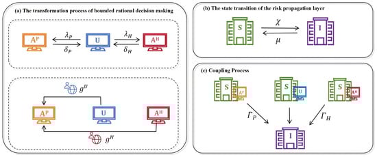
Figure 3. Schematic diagram of state transitions in the coupled dynamics model.

2.3.2. Assumption 2: Time-Varying Adaptive Propagation Rules

The study of information diffusion models in hypernetworks mainly adopts the method based on epidemic models, and the two commonly used methods are global dissemination based on the reactive process (RP) and local dissemination based on the contact process (CP) [38,39,40]. The information propagation process in the real world typically falls between these two extremes, so this paper adopts an adaptive propagation model, which allows for selective propagation of information to neighbors within the hyperedge.

In hypernetworks, the hyperdegree of a node is defined as the number of hyperedges in which the node is involved. The hyperdegree of a node is indicative of the degree of participation of the node in the network. In the threshold model of disease, nodes with higher hyperdegree are more likely to be activated, and the activation speed is faster [41]. In the context of cooperation in multigames, high hyperdegree nodes influence surrounding nodes to form a cooperator cluster, while the groups with a low hyperdegree have a lower degree of cooperation [42]. In the study of rumor propagation, the hyperdegree of nodes is used to replace the degree, and the obtained model reaches equilibrium faster than the general model [43,44].

In this paper, the nodes with large hyperdegree represent the more group interactions that this symbiotic enterprise participates in. The weight of each hyperedge $\left(w\left(e_i\right),i=\mathrm{1,2},\dots ,m\right)$ is assumed to be equal to the sum of the hyperdegrees of the nodes in the hyperedge, and the weight of the hyperedge represents the active degree of the social circle. At each moment, each enterprise first selects an active hyperedge and then exchanges risk information with neighboring nodes in the selected active hyperedge according to the rules in Assumption 1. The probability that hyperedge ${\mathrm{e}}_{\mathrm{j}}$, to which node ${\mathrm{v}}_{\mathrm{i}}$ belongs is selected as an active hyperedge is as follows:

$${\mathrm{p}}_{\mathrm{j},\mathrm{i}}={\displaystyle \frac{\mathrm{w}\left({\mathrm{e}}_{\mathrm{j}}\right)}{\sum _{{\mathrm{e}}_{\mathrm{k}}\in {\mathrm{M}}_{\mathrm{i}}}\mathrm{w}\left({\mathrm{e}}_{\mathrm{k}}\right)}},$$

(10)

where ${\mathrm{M}}_{\mathrm{i}}$ is hyperedge set containing node ${\mathrm{v}}_{\mathrm{i}}$.

It is important to note that social networks are not static entities. Consequently, information dissemination channels are subject to change over time, including the establishment of new social relationships and the dissolution of old ones. Time-varying network models have been demonstrated to capture the dynamic changes in network structures, thereby facilitating a more accurate description of the process of bounded rational decision transformation. Therefore, this paper stipulates that at every moment, the social network undergoes evolution—specifically, the addition and deletion of hyperedges—followed by a shift towards bounded rational decision-making according to the aforementioned adaptive propagation rules. As illustrated in Figure 4, the specific process of bounded rational decision transformation in social networks is demonstrated.

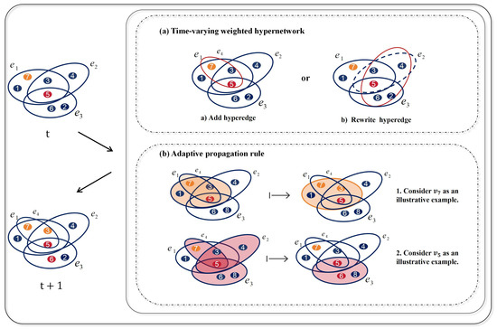
Figure 4. Schematic diagram of state transitions from $\mathrm{t}$ to $\mathrm{t}+1$ according to the time-varying adaptive propagation rule. Node states are categorized as: unaware (blue), aware and hesitant (orange), and aware and positive (red). Panel (a) shows the time-varying process of the hypernetwork, where solid red lines denote newly added hyperedges and dashed blue lines represent removed hyperedges. Panel (b) illustrates the state transition under the adaptive propagation rule (${\mathrm{v}}_7$ is located on hyperedges ${\mathrm{e}}_1$ and ${\mathrm{e}}_4$, the active hyperedge ${\mathrm{e}}_1$ is selected based on the probability shown in Equation (10), and information is exchanged with the neighboring nodes in ${\mathrm{e}}_1$, ultimately changing the state of node ${\mathrm{v}}_3$. Node ${\mathrm{v}}_5$ is similar to).

2.3.3. Assumption 3: Mass Media and Crowd Effects

The mass media serve as the primary and reliable source of risk-related information. However, due to information asymmetry, data acquisition lag, and limited expert interpretation, media reports do not comprehensively cover the scale and severity of risks. We employ $\widetilde{{\mathsf{\rho }}^{\mathrm{I}}}\left(\mathrm{t}\right)$ and ${\mathsf{\rho }}^{\mathrm{I}}\left(\mathrm{t}\right)$ to represent the scale of risk reported by the media and the actual scale of risk at time $\mathrm{t}$, respectively. To describe this difference, this paper introduces a weakening factor $\mathsf{\theta }\left(0\le \mathsf{\theta }\le 1\right)$, allowing $\widetilde{{\mathsf{\rho }}^{\mathrm{I}}}\left(\mathrm{t}\right)=\mathsf{\theta }{\mathsf{\rho }}^{\mathrm{I}}\left(\mathrm{t}\right)$.

In addition, this paper also considers environmental factors, namely the impact of crowd effects on bounded rational decisions. When hesitant firms detect a greater number of proactive symbiotic partners in their vicinity, they may shift towards a risk-positive stance. This paper denotes the crowd effect as ${\mathsf{\xi }}_{\mathrm{i}}\left(\mathrm{t}\right)$. Specifically, firms in state $A^H$ dynamically adjust and update their state at time $t$ based on the state of their neighbors at the previous time step ($t-1$), i.e.,

$${\mathsf{\xi }}_{\mathrm{i}}\left(\mathrm{t}\right)=\mathrm{l}\mathrm{g}\left(1+{\displaystyle \frac{{\sum }_{\mathrm{j}=1}^{\mathrm{N}}{\mathrm{a}}_{\mathrm{j}\mathrm{i}}{\mathrm{P}}_{\mathrm{j}}^{{\mathrm{A}}^{\mathrm{P}}}\left(\mathrm{t}-1\right)}{{\mathrm{k}}_{\mathrm{i}}\left(\mathrm{t}\right)}}\right),$$

(11)

where ${\mathrm{a}}_{\mathrm{j}\mathrm{i}}$ indicates whether nodes ${\mathrm{v}}_{\mathrm{j}}$ and ${\mathrm{v}}_{\mathrm{i}}$ are adjacent in the social network, ${\mathrm{a}}_{\mathrm{j}\mathrm{i}}=1$ indicates that nodes ${\mathrm{v}}_{\mathrm{j}}$ and ${\mathrm{v}}_{\mathrm{i}}$ are adjacent, otherwise ${\mathrm{a}}_{\mathrm{j}\mathrm{i}}=0$. ${\mathrm{k}}_{\mathrm{i}}\left(\mathrm{t}\right)$ indicates the number of nodes adjacent to node ${\mathrm{v}}_{\mathrm{i}}$ at time $\mathrm{t}$. ${\mathrm{P}}_{\mathrm{j}}^{{\mathrm{A}}^{\mathrm{P}}}\left(\mathrm{t}-1\right)$ indicates the probability that node ${\mathrm{v}}_{\mathrm{j}}$ is in state ${\mathrm{A}}^{\mathrm{P}}$ at time $\mathrm{t}-1$.

At the same time, repeated exposure to a piece of information can increase its credibility, meaning that the more times a piece of risk information is repeated, the greater the probability that it will be believed. Therefore, this paper uses $\mathsf{\eta }$ to represent the reinforcement effect of mass media information.

In summary, under the influence of mass media and crowd effects, the probability of symbiotic enterprises changing from states $\mathrm{U}$ and ${\mathrm{A}}^{\mathrm{H}}$ to risk-positive attitudes ${\mathrm{A}}^{\mathrm{P}}$ is defined as decision functions ${\mathrm{g}}_{\mathrm{i}}^{\mathrm{U}}$ and ${\mathrm{g}}_{\mathrm{i}}^{\mathrm{H}}$, respectively.

$$\left\{\begin{array}{l}{\mathrm{g}}_{\mathrm{i}}^{\mathrm{U}}=\mathrm{H}\left(\mathsf{\theta }{\mathsf{\rho }}^{\mathrm{I}}\left(\mathrm{t}\right)·\mathsf{\eta }-\overline{{\mathrm{k}}_{\mathrm{i}}}\left(\mathrm{t}\right)\right)\\ {\mathrm{g}}_{\mathrm{i}}^{\mathrm{H}}=\mathrm{H}\left(\mathsf{\theta }{\mathsf{\rho }}^{\mathrm{I}}\left(\mathrm{t}\right)·\mathsf{\eta }+{\mathsf{\xi }}_{\mathrm{i}}\left(\mathrm{t}\right)-\overline{{\mathrm{k}}_{\mathrm{i}}}\left(\mathrm{t}\right)\right)\end{array}\right.,$$

(12)

where $\mathrm{H}\left(\mathrm{x}\right)$ denotes the step function, $\overline{{\mathrm{k}}_{\mathrm{i}}}\left(\mathrm{t}\right)={\displaystyle \frac{\mathrm{k}}{{\mathrm{k}}_{\mathrm{i}}\left(\mathrm{t}\right)}}$ is the global perception ratio at time $\mathrm{t}$, and $\mathrm{k}\left(0\le \mathrm{k}\le \mathrm{m}\mathrm{a}\mathrm{x}\left({\mathrm{k}}_{\mathrm{i}}\right)\right)$ is the control factor of the global perception ratio.

Figure 5 can help us better understand the influence of mass media and crowd effects on bounded rational decision-making. The second panel of Figure 3a represents the transition of $U$ and $A^H$ states to $A^P$ states according to the decision probabilities $g_i^U$ and $g_i^H$.

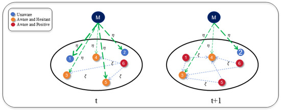
Figure 5. The influence of mass media and crowd effects on bounded rational decision-making processes. Node M represents the Mass media. At time $t$, the unaware nodes $v_1$ and $v_2$ (blue) receive the risk information transmitted by the mass media. The thickness of the green dotted line represents the strength of the reinforcement effect of the mass media information. Nodes $v_3$, $v_4$, and $v_5$ with risk hesitant attitude (orange), in addition to receiving risk information transmitted by mass media (green dashed line), are also affected by the number of surrounding symbiotic partners with positive risk attitude, namely crowd effect (blue dashed line). At time $t+1$, the unaware node $v_1$ and the risk hesitant attitude node $v_5$ become risk-positive (red).

2.3.4. Assumption 4: Risk Transmission Process

In this paper, the $\mathrm{S}\mathrm{I}\mathrm{S}$ epidemic model is used to describe risk propagation in industrial symbiosis networks. Considering that the infection rate, namely the probability of susceptible individuals being infected by their infected neighbors, is always related to the susceptibility (admission rate ${\mathrm{A}}_{\mathrm{i}}$) and infectivity (transmission rate ${\mathrm{T}}_{\mathrm{i}}$) [45]. This paper makes the following assumptions about the risk propagation process.

A company’s risk perception capabilities (the comprehensive ability to identify, assess, and interpret potential risks within a symbiotic network) have a decisive impact on strategic decision-making and crisis response mechanisms [46]. Specifically, enterprises with stronger risk perception capabilities can more accurately quantify the impact of risk events, implement more targeted risk mitigation measures, and more effectively reduce their own risk exposure levels. Additionally, when partners with higher levels of symbiotic dependence encounter risks, the enterprise’s risk acceptance rate will significantly increase. For example, if an enterprise’s sole supplier experiences a production interruption, the enterprise may be unable to quickly find an alternative solution, leading to a higher risk acceptance rate. Therefore, this paper defines the risk acceptance rate of a susceptible enterprise ${\mathrm{v}}_{\mathrm{i}}$ with respect to its infected neighbor ${\mathrm{v}}_{\mathrm{j}}$ as follows:

$${\mathrm{A}}_{\mathrm{i}\mathrm{j}}^{\mathrm{X}}\left(\mathrm{t}\right)=\left\{\begin{array}{l}0\hspace{1em}\hspace{1em}\hspace{1em}\hspace{1em}\hspace{1em}\hspace{1em}\hspace{1em}\hspace{1em}\hspace{1em}\hspace{1em}\hspace{1em}\hspace{1em}\hspace{1em}\hspace{1em}\hspace{1em}\hspace{1em}{\mathsf{\rho }}^{\mathrm{I}}\left(\mathrm{t}\right)\le {\mathsf{\rho }}_0\\ {\mathrm{\phi }}_{\mathrm{i}\mathrm{j}}\left(\mathrm{t}\right)\left(1-{\mathsf{\alpha }}^{\mathrm{X}}\right)\left({\mathsf{\rho }}^{\mathrm{I}}\left(\mathrm{t}\right)-{\mathsf{\rho }}_0\right) {\mathsf{\rho }}_0<{\mathsf{\rho }}^{\mathrm{I}}\left(\mathrm{t}\right)<{\mathsf{\rho }}_{\mathrm{c}}\\ {\mathrm{\phi }}_{\mathrm{i}\mathrm{j}}\left(\mathrm{t}\right)\left(1-{\mathsf{\alpha }}^{\mathrm{X}}\right)\hspace{1em}\hspace{1em}\hspace{1em}\hspace{1em}\hspace{1em}\hspace{1em}\hspace{1em}\hspace{1em}\hspace{1em}{\mathsf{\rho }}^{\mathrm{I}}\left(\mathrm{t}\right)\ge {\mathsf{\rho }}_{\mathrm{c}} \end{array}\right.,$$

(13)

where ${\mathrm{\phi }}_{\mathrm{i}\mathrm{j}}\left(\mathrm{t}\right)$ represents the degree of symbiotic dependence of enterprise ${\mathrm{v}}_{\mathrm{i}}$ to ${\mathrm{v}}_{\mathrm{j}}$ at time $\mathrm{t}$, ${\mathsf{\alpha }}^{\mathrm{X}}$ denotes the risk perception capability of enterprises ${\mathrm{v}}_{\mathrm{i}}$ in state $\mathrm{X}$, with $\mathrm{X}=\left\{\mathrm{U},{\mathrm{A}}^{\mathrm{H}},{\mathrm{A}}^{\mathrm{P}}\right\}$, ${\mathsf{\rho }}_0$ denotes the minimum value of the risk scale that triggers the perception capability of enterprises, ${\mathsf{\rho }}_{\mathrm{c}}$ denotes the specific threshold for triggering firms’ risk perception capabilities, with $0\le {\mathsf{\rho }}_0\le {\mathsf{\rho }}_{\mathrm{c}}\le 1$. When ${\mathsf{\rho }}^{\mathrm{I}}\left(\mathrm{t}\right)\le {\mathsf{\rho }}_0$, susceptible firms are not affected by risk; when ${\mathsf{\rho }}^{\mathrm{I}}\left(\mathrm{t}\right)\ge {\mathsf{\rho }}_{\mathrm{c}}$, the risk admission rate of susceptible firms is no longer influenced by the current risk scale. To calculate the risk propagation threshold, this paper assumes that ${\mathsf{\rho }}_0={\mathsf{\rho }}_{\mathrm{c}}=0$.

The k-shell has the advantages of globality, robustness [47,48] and hierarchical structure [49], and performs better than other metrics in simulations of SIR and SIS models [50]. The k-shell value $\mathrm{k}\_\mathrm{s}$ is a reliable predictor of influential spreaders [51]. During risk propagation, enterprises’ risk transmission capacity is closely related to its position within the network. Therefore, this paper uses Equation (14) containing $\mathrm{k}\_\mathrm{s}$ to express the risk transmission rate ${\mathrm{T}}_{\mathrm{i}}\left(\mathrm{t}\right)$ of the infected enterprise ${\mathrm{v}}_{\mathrm{i}}$ at time $t$.

$${\mathrm{T}}_{\mathrm{i}}\left(\mathrm{t}\right)=\mathsf{\beta }·\left[T_{min}+\left(1-T_{min}\right){\displaystyle \frac{{\mathrm{k}\_\mathrm{s}}_{\mathrm{i}}\left(\mathrm{t}\right)-{{\mathrm{k}}_{\mathrm{s}}}_{\mathrm{m}\mathrm{i}\mathrm{n}}\left(\mathrm{t}\right)}{{\mathrm{k}\_\mathrm{s}}_{\mathrm{m}\mathrm{a}\mathrm{x}}\left(\mathrm{t}\right)-{{\mathrm{k}}_{\mathrm{s}}}_{\mathrm{m}\mathrm{i}\mathrm{n}}\left(\mathrm{t}\right)}}\right]=\mathsf{\beta }·\overline{{\mathrm{k}\_\mathrm{s}}_{\mathrm{i}}}\left(\mathrm{t}\right),$$

(14)

where $\mathsf{\beta }$ is the basic risk propagation rate, ${\mathrm{k}\_\mathrm{s}}_{\mathrm{i}}\left(\mathrm{t}\right)$ is the k-shell value of enterprise ${\mathrm{v}}_{\mathrm{i}}$ at time $\mathrm{t}$, ${\mathrm{k}\_\mathrm{s}}_{\mathrm{m}\mathrm{a}\mathrm{x}}\left(\mathrm{t}\right)$ and ${\mathrm{k}\_\mathrm{s}}_{\mathrm{m}\mathrm{i}\mathrm{n}}\left(\mathrm{t}\right)$ represent the maximum and minimum k-shell values at time $\mathrm{t}$, $T_{min}$ is the minimum risk propagation ability of a node ${\mathrm{v}}_{\mathrm{i}}$, and $T_{min}={10}^{-5}$ is assumed in this paper.

In summary, the infection rate between ${\mathrm{v}}_{\mathrm{i}}$ and ${\mathrm{v}}_{\mathrm{j}}$ is as follows:

$${\mathsf{\chi }}_{\mathrm{i}\mathrm{j}}^{\mathrm{X}}(\mathrm{t})=\left\{\begin{array}{c}{\mathrm{A}}_{\mathrm{i}\mathrm{j}}^{\mathrm{X}}\left(\mathrm{t}\right)·{\mathrm{T}}_{\mathrm{j}}\left(\mathrm{t}\right) {\mathrm{v}}_{\mathrm{i}} \mathrm{is} \mathrm{susceptible} \mathrm{and} {\mathrm{v}}_{\mathrm{j}} \mathrm{is} \mathrm{infectious}\\ {{\mathrm{T}}_{\mathrm{i}}\left(\mathrm{t}\right)·\mathrm{A}}_{\mathrm{j}\mathrm{i}}^{\mathrm{X}}\left(\mathrm{t}\right) {\mathrm{v}}_{\mathrm{i}} \mathrm{is} \mathrm{infectious} \mathrm{and} {\mathrm{v}}_{\mathrm{j}} \mathrm{is} \mathrm{susceptible}\\ 0 \mathrm{otherwise} \end{array}\right.,$$

(15)

where $\mathrm{X}=\left\{\mathrm{U},{\mathrm{A}}^{\mathrm{P}},{\mathrm{A}}^{\mathrm{H}}\right\}$.

Exposed enterprises will return to a susceptible state with probability $\mathsf{\mu }$. The risk propagation process is shown in Figure 3b.

2.3.5. Assumption 5: Coupling Process

Companies that are aware of risk information will constantly monitor the risk situation around them and remain vigilant at all times. This paper introduces the risk perception ability attenuation factors ${\Gamma }_{\mathrm{U}}$ and ${\Gamma }_{\mathrm{H}}$, where $0<{\Gamma }_{\mathrm{U}}<{\Gamma }_{\mathrm{H}}<1$. Companies that take a positive attitude towards risk usually have a higher risk perception ability than the other two states, that is, ${\mathsf{\alpha }}^{\mathrm{P}}>{\mathsf{\alpha }}^{\mathrm{H}}>{\mathsf{\alpha }}^{\mathrm{U}}$, as shown in Figure 3c.

$$\left\{\begin{array}{l}{\mathsf{\alpha }}^{\mathrm{P}}=\mathsf{\alpha }\\ {\mathsf{\alpha }}^{\mathrm{H}}={{\Gamma }_{\mathrm{H}}·\mathsf{\alpha }}^{\mathrm{P}}={\Gamma }_{\mathrm{H}}·\mathsf{\alpha }\\ {\mathsf{\alpha }}^{\mathrm{U}}={{\Gamma }_{\mathrm{U}}·\mathsf{\alpha }}^{\mathrm{P}}={\Gamma }_{\mathrm{U}}·\mathsf{\alpha }\end{array}\right.,$$

(16)

Additionally, this paper proposes a nonlinear coupling relationship, where the transition parameters in one layer are influenced not only by the node states in another layer but also by the topological properties of nodes in another layer. In other words, the topological structure of ISN affects the bounded rational decisions of enterprises. Specifically, the more common partners two symbiotic enterprises have, the more similar their status and roles in ISN are, and the higher the possibility that they belong to the same industry or have similar production directions. Enterprises with high similarity may have similar production models, technical routes, or market strategies, so it is easier for them to understand and accept each other’s decisions about risk information, thereby affecting the change in bounded rational decisions. See Equation (30) for a detailed expression.

2.3.6. Assumption 6: Time-Delay Effect

The formation of bounded rational decisions by enterprises requires a series of processes, such as information acquisition, information interpretation, and risk assessment, which essentially constitute a time delay in risk information perception [52,53]. This paper compares the moment of risk infection with that of bounded rational decision to more accurately describe the dynamic characteristics of risk evolution in industrial symbiosis networks. The model introduces the decision incubation period function ${\mathsf{\tau }}_{\mathrm{i}}$, which satisfies an exponential distribution with mean $\mathsf{\nu }$. Since this paper is based on a discrete Markov chain model, ${\mathsf{\tau }}_{\mathrm{i}}$ is rounded to the nearest integer for convenience. The three following main situations can be derived:

• Scenario 1: ${\mathsf{\tau }}_{\mathrm{i}}\le 1$. Once an enterprise is infected with risk, it will immediately make a bounded rational decision (${\mathrm{A}}^{\mathrm{P}}$), that is, it will directly transition from state $\mathrm{U}\mathrm{I}$ and ${\mathrm{A}}^{\mathrm{H}}\mathrm{I}$ to ${\mathrm{A}}^{\mathrm{P}}\mathrm{I}$. There are only four states in the system: $\mathrm{U}\mathrm{S}$, ${\mathrm{A}}^{\mathrm{H}}\mathrm{S}$, ${\mathrm{A}}^{\mathrm{P}}\mathrm{S}$ and ${\mathrm{A}}^{\mathrm{P}}\mathrm{I}$. The corresponding state transition probability tree can be seen in Figure 6;
  

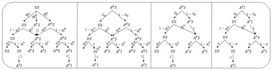  Figure 6. State transition probability tree when ${\mathsf{\tau }}_{\mathrm{i}}\le 1$.
• Scenario 2: $1<\mathrm{t}<{\mathsf{\tau }}_{\mathrm{i}}$. Once a company in the $\mathrm{U}\mathrm{S}$, ${\mathrm{A}}^{\mathrm{H}}\mathrm{S}$ state is infected, it will enter incubation period and remain in $\mathrm{U}\mathrm{I}$ and ${\mathrm{A}}^{\mathrm{H}}\mathrm{I}$ states. The corresponding state transition probability tree is shown in Figure 7 (excluding the red dotted arrow);
  

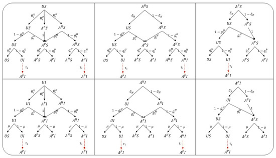  Figure 7. State transition probability tree when $1<\mathrm{t}<{\mathsf{\tau }}_{\mathrm{i}}$ (excluding the red dotted arrow) and $1<{\mathsf{\tau }}_{\mathrm{i}}\le \mathrm{t}$ (including the red dotted arrow).
• Scenario 3: $1<{\mathsf{\tau }}_{\mathrm{i}}\le \mathrm{t}$. The incubation period is over, and companies in the $\mathrm{U}\mathrm{I}$ and ${\mathrm{A}}^{\mathrm{H}}\mathrm{I}$ states realize the risks and make bounded rational decisions, that is, they shift to the ${\mathrm{A}}^{\mathrm{P}}\mathrm{I}$ state. The corresponding state transition probability tree is shown in Figure 7 (including the red dotted arrow).

3. Theory Analysis

3.1. Theoretical Analysis of Hyperdegree Evolution

In this section, the mean theory [54,55] is used to analyze the hyperdegree distribution of the hypernetwork model constructed according to the hyperdegree priority connection mechanism proposed in Section 2.2.1. Supposing that $h_j\left(t,t_i\right)$ is a continuous real variable. It can be seen that $h_j\left(t,t_i\right)$ satisfies the following dynamical equations.

[1]

New node batches are added with probability ${\mathrm{q}}_1$,

$${\displaystyle \frac{\partial h_j\left(t,t_i\right)}{\partial t}}=q_1{m}_{1}b{\lambda }^{\prime }{\displaystyle \frac{h_j\left(t,t_i\right)}{\sum _{i,j}{h}_j\left(t,t_i\right)}},$$

(17)

[2]

New hyperedges are added with probability ${\mathrm{q}}_2$,

$${\displaystyle \frac{\partial h_j\left(t,t_i\right)}{\partial t}}=q_2{m}_2\left({\displaystyle \frac{1}{N_t}}+b{\displaystyle \frac{h_j\left(t,t_i\right)}{\sum _{i,j}{h}_j\left(t,t_i\right)}}\right).$$

(18)

[3]

Existing hyperedges are reconnect with probability ${\mathrm{q}}_3$,

$${\displaystyle \frac{\partial h_j\left(t,t_i\right)}{\partial t}}=q_3{m}_3\left(-{\displaystyle \frac{1}{N_t}}+b{\displaystyle \frac{h_j\left(t,t_i\right)}{\sum _{i,j}{h}_j\left(t,t_i\right)}}\right).$$

(19)

where ${\mathrm{N}}_{\mathrm{t}}$ denotes the total number of nodes at time $\mathrm{t}$, and $\underset{t\to \infty }{\mathit{lim}}{N}_t=q_1\overline{a}{\lambda }^{\prime }t$.

Combining Equations (17)–(19), we can achieve

$${\displaystyle \frac{\partial h_j\left(t,t_i\right)}{\partial t}}=q_1{m}_{1}b{\lambda }^{\prime }{\displaystyle \frac{h_j\left(t,t_i\right)}{\sum _{i,j}{h}_j\left(t,t_i\right)}}+\left(q_2{m}_2+q_3{m}_3\right)b{\displaystyle \frac{h_j\left(t,t_i\right)}{\sum _{i,j}{h}_j\left(t,t_i\right)}}+{\displaystyle \frac{q_2{m}_2-q_3{m}_3}{N_t}}.$$

(20)

Since the arrival of node batches follows a Poisson distribution $\mathrm{N}\left(\mathrm{t}\right)$ with rate ${\mathsf{\lambda }}^{\prime }$, then $\mathrm{E}\left(\mathrm{N}\left(\mathrm{t}\right)\right)={\mathrm{q}}_1{\mathsf{\lambda }}^{\prime }\mathrm{t}$. Let

$$x=\underset{t\to \infty }{\mathit{lim}}{\displaystyle \frac{1}{q_1{\lambda }^{\prime }t}}\sum _{i,j}{h}_j\left(t,t_i\right),$$

(21)

then we have,

$${\displaystyle \frac{\partial h_j\left(t,t_i\right)}{\partial t}}=m_{1}b{\displaystyle \frac{h_j\left(t,t_i\right)}{xt}}+\left(q_2{m}_2+q_3{m}_3\right)b{\displaystyle \frac{h_j\left(t,t_i\right)}{x{q}_1{\lambda }^{\prime }t}}+{\displaystyle \frac{q_2{m}_2-q_3{m}_3}{q_1\overline{a}{\lambda }^{\prime }t}}.$$

(22)

Let $\mathrm{A}={\displaystyle \frac{{\mathrm{m}}_1\mathrm{b}}{\mathrm{x}}}+{\displaystyle \frac{({\mathrm{q}}_2{\mathrm{m}}_2-{\mathrm{q}}_3{\mathrm{m}}_3)\mathrm{b}}{\mathrm{x}{\mathrm{q}}_1{\mathsf{\lambda }}^{\prime }}}, \mathrm{B}={\displaystyle \frac{{\mathrm{q}}_2{\mathrm{m}}_2-{\mathrm{q}}_3{\mathrm{m}}_3}{{\mathrm{q}}_1\overline{\mathrm{a}}{\mathsf{\lambda }}^{\prime }}}$, the solution of Equation (22), with the initial condition that a node in the $\mathrm{i}$ th batch at its birth time satisfies ${\mathrm{h}}_{\mathrm{j}}\left(\mathrm{t},{\mathrm{t}}_{\mathrm{i}}\right)={\mathrm{m}}_1$, is

$$h_j\left(t,t_i\right)=\left(m_1+{\displaystyle \frac{B}{A}}\right){\left({\displaystyle \frac{t}{t_i}}\right)}^A-{\displaystyle \frac{B}{A}},j=\mathrm{1,2},3,\dots ,a_i,$$

(23)

where $\mathrm{x}$ satisfies the following equation,

$$x={\displaystyle \frac{1}{q_1{\lambda }^{\prime }t}}\int g\left(b\right)db\int \left[\left(m_1+{\displaystyle \frac{B}{A}}\right){\left({\displaystyle \frac{t}{t_i}}\right)}^A-{\displaystyle \frac{B}{A}}\right]dt.$$

(24)

It can be seen from Equation (23) that

$$P\left(h_j\left(t,t_i\right)\ge k\right)=P\left(t_i\le t·{\left({\displaystyle \frac{kA+B}{m_{1}A+B}}\right)}^{-{\displaystyle \frac{1}{A}}}\right),$$

(25)

Because $t_i$ follows the gamma distribution $\left(i,{\lambda }^{\prime }\right)$, that is,

$$P\left(t_i\le x\right)=1-e^{-{\lambda }^{\prime }x}\sum _{l=0}^{i-1}{\displaystyle \frac{({\lambda }^{\prime }x{)}^l}{l!}},$$

(26)

then

$$P\left(h_j\left(t,t_i\right)\ge k\right)=1-e^{-{\lambda }^{\prime }·t·{\left({\displaystyle \frac{kA+B}{m_{1}A+B}}\right)}^{-{\displaystyle \frac{1}{A}}}}·\sum _{l=0}^{i-1}{\displaystyle \frac{1}{l!}}{\left[{\lambda }^{\prime }t·{\left({\displaystyle \frac{kA+B}{m_{1}A+B}}\right)}^{-{\displaystyle \frac{1}{A}}}\right]}^l,$$

(27)

The final result is

$$P\left(h_j\left(t,t_i\right)=k\right)\approx {\displaystyle \frac{\partial P\left(h_j\left(t,t_i\right)<k\right)}{\partial k}}={\displaystyle \frac{{\lambda }^{\prime }t}{m_{1}A+B}}{\left({\displaystyle \frac{B+Ak}{m_{1}A+B}}\right)}^{-{\displaystyle \frac{1}{A}}-1}{e}^{-{\lambda }^{\prime }·t·{\left({\displaystyle \frac{kA+B}{m_{1}A+B}}\right)}^{-{\displaystyle \frac{1}{A}}}}{\displaystyle \frac{1}{\left(i-1\right)!}}{\left[{\lambda }^{\prime }t·{\left({\displaystyle \frac{kA+B}{m_{1}A+B}}\right)}^{-{\displaystyle \frac{1}{A}}}\right]}^{i-1}$$

(28)

Therefore, the hyperdegree distribution in a stable state satisfies:

$$P\left(k\right)=\int P\left(h_j\left(t,t_i\right)=k\right)g\left(b\right)db.$$

(29)

3.2. Theoretical Analysis Based on MMCA

MMCA has been widely used to analyze the propagation dynamics of coevolution [56,57]. In this section, MMCA is applied to analyze the risk propagation process and calculate the risk propagation threshold.

The state of an enterprise ${\mathrm{v}}_{\mathrm{i}}$ may be one of $US$, $A^{H}S$, $A^{P}S$, $UI$, $A^{H}I$, and $A^{P}I$ at each time step $\mathrm{t}$, and the corresponding probabilities at these states are set to be $P_i^{US}\left(t\right)$, $P_i^{A^{H}S}\left(t\right)$, $P_i^{A^{P}S}\left(t\right)$, $P_i^{UI}\left(t\right)$, $P_i^{A^{H}I}\left(t\right)$, and $P_i^{A^{P}I}\left(t\right)$, respectively. In this paper, we use ${\gamma }_i^P\left(t\right)$ and ${\gamma }_i^H\left(t\right)$ to denote the probability that risk-unaware enterprises do not receive risk information transmitted by neighbors with hesitant or positive attitudes, respectively.

$$\left\{\begin{array}{c}{\gamma }_i^H\left(t\right)={\displaystyle \prod _{j\ne i}}\left[1-a_{ji}{P}_i^H\left(t\right)J_{ij}{\omega }_j{\lambda }_H\right]\\ {\gamma }_i^P\left(t\right)={\displaystyle \prod _{j\ne i}}\left[1-a_{ji}{P}_i^P\left(t\right)J_{ij}{\omega }_j{\lambda }_P\right]\end{array}\right.,$$

(30)

where $P_i^H\left(t\right)=P_i^{A^{H}S}\left(t\right)+P_i^{A^{H}I}\left(t\right)$, $P_i^P\left(t\right)=P_i^{A^{P}S}\left(t\right)+P_i^{A^{P}I}\left(t\right)$, $J_{ij}$ denotes similarity between ${\mathrm{v}}_{\mathrm{i}}$ and ${\mathrm{v}}_{\mathrm{j}}$.

It is worth noting that when enterprise $v_i$ receives risk information from symbiotic neighbors in both states $A^H$ and $A^P$, it will only accept one view. This paper further introduces ${\Theta }_i^H\left(t\right)$ and ${\Theta }_i^P\left(t\right)$ to represent the probability that risk-unaware enterprises adopt a risk-hesitant attitude and a proactive attitude, respectively, while ${\Theta }_i^U\left(t\right)$ represents the probability that risk-unaware enterprises remain unaware.

$$\left\{\begin{array}{l}{\Theta }_i^U\left(t\right)={\gamma }_i^P\left(t\right)·{\gamma }_i^H\left(t\right) \\ {\Theta }_i^H\left(t\right)=1-{\gamma }_i^H\left(t\right)-\left(1-\epsilon \right)\left(1-{\gamma }_i^P\left(t\right)\right)\left(1-{\gamma }_i^H\left(t\right)\right) \\ {\Theta }_i^P\left(t\right)=1-{\gamma }_i^P\left(t\right)-\epsilon \left(1-{\gamma }_i^P\left(t\right)\right)\left(1-{\gamma }_i^H\left(t\right)\right)\end{array}\right.,$$

(31)

where $\mathsf{\epsilon }\left(0\le \mathsf{\epsilon }\le 1\right)$ is the preference value for hesitant attitudes.

In the risk transmission layer, all infected neighbors of susceptible enterprises may transmit risk to them. Therefore, the probabilities that enterprises in states $\mathrm{U}\mathrm{S}$, ${\mathrm{A}}^{\mathrm{H}}\mathrm{S}$ and ${\mathrm{A}}^{\mathrm{P}}\mathrm{S}$ are not infected by symbiotic neighbors are represented as follows:

$$\left\{\begin{array}{c}{q}_i^U\left(t\right)={\displaystyle \prod _{j\ne i}}\left[1-b_{ji}{P}_j^I\left(t\right){\chi }_{ij}^U\left(t\right)\right]\\ q_i^P\left(t\right)={\displaystyle \prod _{j\ne i}}\left[1-b_{ji}{P}_j^I\left(t\right){\chi }_{ij}^P\left(t\right)\right]\\ q_i^H\left(t\right)={\displaystyle \prod _{j\ne i}}\left[1-b_{ji}{P}_j^I\left(t\right){\chi }_{ij}^H\left(t\right)\right]\end{array}\right.,$$

(32)

where $P_j^I\left(t\right)=P_j^{UI}\left(t\right)+P_j^{A^{H}I}\left(t\right)+P_j^{A^{P}I}\left(t\right)$, $b_{ji}$ denotes the $j$-row and $i$-column element of the adjacency matrix of ISN, in which $b_{ji}=1$ indicates that nodes $v_j$ and $v_i$ are neighbors, otherwise $b_{ji}=0$.

The transition probabilities of node states under different incubation periods are calculated as follows:

• Scenario 1: ${\tau }_i\le 1$. There are only four states in the network: $US$, $A^{H}S$, $A^{P}S,$ and $A^{P}I$, and the evolution equations can be expressed as follows:

  $$\left\{\begin{array}{l}{P}_i^{US}\left(t+1\right)=P_i^{US}\left(t\right){\Theta }_i^U\left(t\right)\left(1-g_i^U\left(t\right)\right)q_i^U\left(t\right)+P_i^{A^{H}S}\left(t\right){\delta }_H\left(1-g_i^U\left(t\right)\right)q_i^U\left(t\right)\\ \hspace{1em}\hspace{1em}\hspace{1em}\hspace{1em}\hspace{1em}\hspace{1em}\hspace{1em}\hspace{1em}\hspace{1em}+P_i^{A^{P}S}\left(t\right){\delta }_P\left(1-g_i^U\left(t\right)\right)q_i^U\left(t\right)+P_i^{A^{P}I}\left(t\right){\delta }_P\left(1-g_i^U\left(t\right)\right)\mu \\ P_i^{A^{H}S}\left(t+1\right)=P_i^{US}\left(t\right){\Theta }_i^H\left(t\right)\left(1-g_i^H\left(t\right)\right)q_i^H\left(t\right)+P_i^{A^{H}S}\left(t\right)\left(1-{\delta }_H\right)\left(1-g_i^H\left(t\right)\right)q_i^H\left(t\right)\\ P_i^{A^{P}S}\left(t+1\right)=P_i^{US}\left(t\right)\left[{\Theta }_i^U\left(t\right)g_i^U\left(t\right)+{\Theta }_i^H\left(t\right)g_i^H\left(t\right)+{\Theta }_i^P\left(t\right)\right]q_i^P\left(t\right)+P_i^{A^{P}S}\left(t\right)\left[{\delta }_P{g}_i^U\left(t\right)+\left(1-{\delta }_P\right)\right]q_i^P\left(t\right)\\ \hspace{1em}\hspace{1em}\hspace{1em}\hspace{1em}\hspace{1em}+P_i^{A^{H}S}\left(t\right)\left[{\delta }_H{g}_i^U\left(t\right)+\left(1-{\delta }_H\right)g_i^H\left(t\right)\right]q_i^P\left(t\right)+P_i^{A^{P}I}\left(t\right)\left[{\delta }_P{g}_i^U\left(t\right)+\left(1-{\delta }_P\right)\right]\mu \\ P_i^{A^{P}I}\left(t+1\right)=P_i^{US}\left(t\right)\left\{\begin{array}{c}{\Theta }_i^U\left(t\right)\left(1-g_i^U\left(t\right)\right)\left(1-q_i^U\left(t\right)\right)+{\Theta }_i^H\left(t\right)\left(1-g_i^H\left(t\right)\right)\left(1-q_i^H\left(t\right)\right)\\ +\left[{\Theta }_i^U\left(t\right)g_i^U\left(t\right)+{\Theta }_i^H\left(t\right)g_i^H\left(t\right)+{\Theta }_i^P\left(t\right)\right]\left(1-q_i^P\left(t\right)\right)\end{array}\right\}\\ \hspace{1em}\hspace{1em}\hspace{1em}\hspace{1em}\hspace{1em}+P_i^{A^{P}S}\left(t\right)\left\{{\delta }_P\left(1-g_i^U\left(t\right)\right)\left(1-q_i^U\left(t\right)\right)+\left[{\delta }_P{g}_i^U\left(t\right)+\left(1-{\delta }_P\right)\right]\left(1-q_i^P\left(t\right)\right)\right\}\\ \hspace{1em}\hspace{1em}\hspace{1em}\hspace{1em}\hspace{1em}+P_i^{A^{H}S}\left(t\right)\left\{\begin{array}{c}{\delta }_H\left(1-g_i^U\left(t\right)\right)\left(1-q_i^U\left(t\right)\right)+\left(1-{\delta }_H\right)\left(1-g_i^H\left(t\right)\right)\left(1-q_i^H\left(t\right)\right)\\ +\left[{\delta }_H{g}_i^U\left(t\right)+\left(1-{\delta }_H\right)\right]\left(1-q_i^P\left(t\right)\right)\end{array}\right\}\\ \hspace{1em}\hspace{1em}\hspace{1em}\hspace{1em}\hspace{1em}\hspace{1em}{+P}_i^{A^{P}I}\left(t\right)\left\{{\delta }_P\left(1-g_i^U\left(t\right)\right)\left(1-\mu \right)+\left[{\delta }_P{g}_i^U\left(t\right)+\left(1-{\delta }_P\right)\right]\left(1-\mu \right)\right\}\\ i\in \left\{\mathrm{1,2},\dots ,N\right\}\end{array},\right.$$

  (33)
• Scenario 2: $1<\mathrm{t}<{\mathsf{\tau }}_{\mathrm{i}}$. There are six states in the network: $US$, $A^{H}S$, $A^{P}S$, $UI$, $A^{H}I,$ and $A^{P}I$, and the evolution equations can be expressed as

  $$\left\{\begin{array}{l}{P}_i^{US}\left(t+1\right)=P_i^{US}\left(t\right){\Theta }_i^U\left(t\right)\left(1-g_i^U\left(t\right)\right)q_i^U\left(t\right)+P_i^{A^{H}S}\left(t\right){\delta }_H\left(1-g_i^U\left(t\right)\right)q_i^U\left(t\right)+P_i^{A^{P}S}\left(t\right){\delta }_P\left(1-g_i^U\left(t\right)\right)q_i^U\left(t\right)\\ \hspace{1em}\hspace{1em}\hspace{1em}\hspace{1em}\hspace{1em}\hspace{1em}+P_i^{UI}\left(t\right){\Theta }_i^U\left(t\right)\left(1-g_i^U\left(t\right)\right)\mu +P_i^{A^{H}I}\left(t\right){\delta }_H\left(1-g_i^U\left(t\right)\right)\mu +P_i^{A^{P}I}\left(t\right){\delta }_P\left(1-g_i^U\left(t\right)\right)\mu \\ P_i^{A^{H}S}\left(t+1\right)=P_i^{US}\left(t\right){\Theta }_i^H\left(t\right)\left(1-g_i^H\left(t\right)\right)q_i^H\left(t\right)+P_i^{A^{H}S}\left(t\right)\left(1-{\delta }_H\right)\left(1-g_i^H\left(t\right)\right)q_i^H\left(t\right)\\ \hspace{1em}\hspace{1em}\hspace{1em}\hspace{1em}\hspace{1em}\hspace{1em}+P_i^{UI}\left(t\right){\Theta }_i^H\left(t\right)\left(1-g_i^H\left(t\right)\right)\mu +P_i^{A^{H}I}\left(t\right)\left(1-{\delta }_H\right)\left(1-g_i^H\left(t\right)\right)\mu \\ P_i^{A^{P}S}\left(t+1\right)=P_i^{US}\left(t\right)\left[{\Theta }_i^U\left(t\right)g_i^U\left(t\right)+{\Theta }_i^H\left(t\right)g_i^H\left(t\right)+{\Theta }_i^P\left(t\right)\right]q_i^P\left(t\right)+P_i^{A^{P}S}\left(t\right)\left[{\delta }_P{g}_i^U\left(t\right)+\left(1-{\delta }_P\right)\right]q_i^P\left(t\right)\\ \hspace{1em}\hspace{1em}\hspace{1em}\hspace{1em}\hspace{1em}\hspace{1em}+P_i^{A^{H}S}\left(t\right)\left[{\delta }_H{g}_i^U\left(t\right)+\left(1-{\delta }_H\right)g_i^H\left(t\right)\right]q_i^P\left(t\right)+P_i^{UI}\left(t\right)\left[{\Theta }_i^U\left(t\right)g_i^U\left(t\right)+{\Theta }_i^H\left(t\right)g_i^H\left(t\right)+{\Theta }_i^P\left(t\right)\right]\mu \\ \hspace{1em}\hspace{1em}\hspace{1em}\hspace{1em}\hspace{1em}\hspace{1em}+P_i^{A^{H}I}\left(t\right)\left[{\delta }_H{g}_i^U\left(t\right)+\left(1-{\delta }_H\right)g_i^H\left(t\right)\right]\mu +P_i^{A^{P}I}\left(t\right)\left[{\delta }_P{g}_i^U\left(t\right)+\left(1-{\delta }_P\right)\right]\mu \\ P_i^{UI}\left(t+1\right)=P_i^{US}\left(t\right){\Theta }_i^U\left(t\right)\left(1-g_i^U\left(t\right)\right)\left(1-q_i^U\left(t\right)\right)+P_i^{A^{H}S}\left(t\right){\delta }_H\left(1-g_i^U\left(t\right)\right)\left(1-q_i^U\left(t\right)\right)\\ \hspace{1em}\hspace{1em}\hspace{1em}\hspace{1em}\hspace{1em}\hspace{1em}+P_i^{A^{P}S}\left(t\right){\delta }_P\left(1-g_i^U\left(t\right)\right)\left(1-q_i^U\left(t\right)\right)+P_i^{UI}\left(t\right){\Theta }_i^U\left(t\right)\left(1-g_i^U\left(t\right)\right)\left(1-\mu \right)\\ \hspace{1em}\hspace{1em}\hspace{1em}\hspace{1em}\hspace{1em}\hspace{1em}+P_i^{A^{H}I}\left(t\right){\delta }_H\left(1-g_i^U\left(t\right)\right)\left(1-\mu \right)+P_i^{A^{P}I}\left(t\right){\delta }_P\left(1-g_i^U\left(t\right)\right)\left(1-\mu \right)\\ P_i^{A^{H}I}\left(t+1\right)=P_i^{US}\left(t\right){\Theta }_i^H\left(t\right)\left(1-g_i^H\left(t\right)\right)\left(1-q_i^H\left(t\right)\right)+P_i^{A^{H}S}\left(t\right)\left(1-{\delta }_H\right)\left(1-g_i^H\left(t\right)\right)\left(1-q_i^H\left(t\right)\right)\\ \hspace{1em}\hspace{1em}\hspace{1em}\hspace{1em}\hspace{1em}\hspace{1em}+P_i^{UI}\left(t\right){\Theta }_i^H\left(t\right)\left(1-g_i^H\left(t\right)\right)\left(1-\mu \right)+P_i^{A^{H}I}\left(t\right)\left(1-{\delta }_H\right)\left(1-g_i^H\left(t\right)\right)\left(1-\mu \right)\\ P_i^{A^{P}I}\left(t+1\right)=P_i^{US}\left(t\right)\left[{\Theta }_i^U\left(t\right)g_i^U\left(t\right)+{\Theta }_i^H\left(t\right)g_i^H\left(t\right)+{\Theta }_i^P\left(t\right)\right]\left(1-q_i^P\left(t\right)\right)+P_i^{A^{H}S}\left(t\right)\left[{\delta }_H{g}_i^U\left(t\right)+\left(1-{\delta }_H\right)g_i^H\left(t\right)\right]\left(1-q_i^P\left(t\right)\right)\\ \hspace{1em}\hspace{1em}\hspace{1em}\hspace{1em}\hspace{1em}\hspace{1em}+P_i^{A^{P}S}\left(t\right)\left[{\delta }_P{g}_i^U\left(t\right)+\left(1-{\delta }_P\right)\right]\left(1-q_i^P\left(t\right)\right)+P_i^{UI}\left(t\right)\left[{\Theta }_i^U\left(t\right)g_i^U\left(t\right)+{\Theta }_i^H\left(t\right)g_i^H\left(t\right)+{\Theta }_i^P\left(t\right)\right]\left(1-\mu \right)\\ \hspace{1em}\hspace{1em}\hspace{1em}\hspace{1em}\hspace{1em}\hspace{1em}+P_i^{A^{H}I}\left(t\right)\left[{\delta }_H{g}_i^U\left(t\right)+\left(1-{\delta }_H\right)g_i^H\left(t\right)\right]\left(1-\mu \right)++P_i^{A^{P}I}\left(t\right)\left[{\delta }_P{g}_i^U\left(t\right)+\left(1-{\delta }_P\right)\right]\left(1-\mu \right)\\ i\in \left\{\mathrm{1,2},\dots ,N\right\}\end{array}\right.$$

  (34)
• Scenario 3: $1<{\mathsf{\tau }}_{\mathrm{i}}\le \mathrm{t}$. The transformation equations in $UI$, $A^{H}I,$ and $A^{P}I$ are different from that of Equation (33), represented as follows:

  $$\left\{\begin{array}{l}{P}_i^{UI}\left(t+1\right)=P_i^{US}\left(t\right){\Theta }_i^U\left(t\right)\left(1-g_i^U\left(t\right)\right)\left(1-q_i^U\left(t\right)\right)+P_i^{A^{H}S}\left(t\right){\delta }_H\left(1-g_i^U\left(t\right)\right)\left(1-q_i^U\left(t\right)\right)\\ \hspace{1em}\hspace{1em}\hspace{1em}\hspace{1em}\hspace{1em}\hspace{1em}+P_i^{A^{P}S}\left(t\right){\delta }_P\left(1-g_i^U\left(t\right)\right)\left(1-q_i^U\left(t\right)\right)+P_i^{UI}\left(t\right){\Theta }_i^U\left(t\right)\left(1-g_i^U\left(t\right)\right)\left(1-\mu \right)\\ \hspace{1em}\hspace{1em}\hspace{1em}\hspace{1em}\hspace{1em}\hspace{1em}+P_i^{A^{H}I}\left(t\right){\delta }_H\left(1-g_i^U\left(t\right)\right)\left(1-\mu \right)+P_i^{A^{P}I}\left(t\right){\delta }_P\left(1-g_i^U\left(t\right)\right)\left(1-\mu \right)\\ \hspace{1em}\hspace{1em}\hspace{1em}\hspace{1em}\hspace{1em}\hspace{1em}-P_i^{UI}\left(t-{\tau }_i+1\right){\displaystyle \prod _{k=t-{\tau }_i+1}^t}{\Theta }_i^U\left(k\right)\left(1-g_i^U\left(k\right)\right)\left(1-\mu \right)-P_i^{A^{H}I}\left(t-{\tau }_i+1\right){\displaystyle \prod _{k=t-{\tau }_i+1}^t}{\delta }_H\left(1-g_i^U\left(k\right)\right)\left(1-\mu \right)\\ P_i^{A^{H}I}\left(t+1\right)=P_i^{US}\left(t\right){\Theta }_i^H\left(t\right)\left(1-g_i^H\left(t\right)\right)\left(1-q_i^H\left(t\right)\right)+P_i^{A^{H}S}\left(t\right)\left(1-{\delta }_H\right)\left(1-g_i^H\left(t\right)\right)\left(1-q_i^H\left(t\right)\right)\\ \hspace{1em}\hspace{1em}\hspace{1em}\hspace{1em}\hspace{1em}\hspace{1em}\hspace{1em}\hspace{1em}\hspace{1em}\hspace{1em}+P_i^{UI}\left(t\right){\Theta }_i^H\left(t\right)\left(1-g_i^H\left(t\right)\right)\left(1-\mu \right)+P_i^{A^{H}I}\left(t\right)\left(1-{\delta }_H\right)\left(1-g_i^H\left(t\right)\right)\left(1-\mu \right)\\ \hspace{1em}\hspace{1em}\hspace{1em}\hspace{1em}\hspace{1em}\hspace{1em}-P_i^{UI}\left(t-{\tau }_i+1\right){\displaystyle \prod _{k=t-{\tau }_i+1}^t}{\Theta }_i^H\left(k\right)\left(1-g_i^H\left(k\right)\right)\left(1-\mu \right)-P_i^{A^{H}I}\left(t-{\tau }_i+1\right){\displaystyle \prod _{k=t-{\tau }_i+1}^t}\left(1-{\delta }_H\right)\left(1-g_i^H\left(k\right)\right)\left(1-\mu \right)\\ P_i^{A^{P}I}\left(t+1\right)=P_i^{US}\left(t\right)\left[{\Theta }_i^U\left(t\right)g_i^U\left(t\right)+{\Theta }_i^H\left(t\right)g_i^H\left(t\right)+{\Theta }_i^P\left(t\right)\right]\left(1-q_i^P\left(t\right)\right)+P_i^{A^{H}S}\left(t\right)\left[{\delta }_H{g}_i^U\left(t\right)+\left(1-{\delta }_H\right)g_i^H\left(t\right)\right]\left(1-q_i^P\left(t\right)\right)\\ \hspace{1em}\hspace{1em}\hspace{1em}\hspace{1em}\hspace{1em}\hspace{1em}+P_i^{A^{P}S}\left(t\right)\left[{\delta }_P{g}_i^U\left(t\right)+\left(1-{\delta }_P\right)\right]\left(1-q_i^P\left(t\right)\right)+P_i^{UI}\left(t\right)\left[{\Theta }_i^U\left(t\right)g_i^U\left(t\right)+{\Theta }_i^H\left(t\right)g_i^H\left(t\right)+{\Theta }_i^P\left(t\right)\right]\left(1-\mu \right)\\ \hspace{1em}\hspace{1em}\hspace{1em}\hspace{1em}\hspace{1em}\hspace{1em}{+P}_i^{A^{H}I}\left(t\right)\left[{\delta }_H{g}_i^U\left(t\right)+\left(1-{\delta }_H\right)g_i^H\left(t\right)\right]\left(1-\mu \right)+P_i^{A^{P}I}\left(t\right)\left[{\delta }_P{g}_i^U\left(t\right)+\left(1-{\delta }_P\right)\right]\left(1-\mu \right)\\ \hspace{1em}\hspace{1em}\hspace{1em}\hspace{1em}\hspace{1em}\hspace{1em}+P_i^{UI}\left(t-{\tau }_i+1\right){\displaystyle \prod _{k=t-{\tau }_i+1}^t}{\Theta }_i^U\left(k\right)\left(1-g_i^U\left(k\right)\right)\left(1-\mu \right)+P_i^{A^{H}I}\left(t-{\tau }_i+1\right){\displaystyle \prod _{k=t-{\tau }_i+1}^t}{\delta }_H\left(1-g_i^U\left(k\right)\right)\left(1-\mu \right)\\ \hspace{1em}\hspace{1em}\hspace{1em}\hspace{1em}\hspace{1em}\hspace{1em}+P_i^{UI}\left(t-{\tau }_i+1\right){\displaystyle \prod _{k=t-{\tau }_i+1}^t}{\Theta }_i^H\left(k\right)\left(1-g_i^H\left(k\right)\right)\left(1-\mu \right)+P_i^{A^{H}I}\left(t-{\tau }_i+1\right){\displaystyle \prod _{k=t-{\tau }_i+1}^t}\left(1-{\delta }_H\right)\left(1-g_i^H\left(k\right)\right)\left(1-\mu \right)\end{array}\right.,$$

  (35)

The risk propagation threshold ${\beta }_c$ determines whether the risk outbreaks or dies out. The epidemic threshold βc follows the rule that, if ${\beta \ge \beta }_c$, the risk will persist in the ISN, and the risk will die out [58] when ${\beta <\beta }_c$.

Theorem 1.

When $t\to \infty$, the risk propagation threshold can be expressed as follows:

$${\beta }_c={\displaystyle \frac{\mu }{{\Lambda }_{max}\left(H\right)}},$$

(36)

where ${\Lambda }_{max}\left(H\right)$ is the maximum eigenvalue of matrix $H={\left(h_{ij}\right)}_{N\times N}$ with  $h_{ij}=\left[1-\alpha \left[1-\left(1-{\mathit{\Gamma }}_U\right)P_i^U-\left(1-{\mathit{\Gamma }}_H\right)P_i^H\right]\right]{\phi }_{ij}\overline{{k\_s}_j}{b}_{ij}$.

Proof. 

The steady state equations of each states can be written as $P_i^X\left(t+1\right)=P_i^X\left(t\right)=P_i^X$, where $X=\left\{US,A^{H}S,A^{P}S,UI,A^{H}I,A^{P}I\right\}$. When approaches the risk propagation threshold, the proportion of infected enterprises could be assumed ${\epsilon }_j=P_j^I=P_j^{UI}+P_j^{A^{H}I}+P_j^{A^{P}I}\ll 1$. Therefore, Equation (32) can be approximated by $q_i^X\approx 1-\sum _{j\ne i}{b}_{ji}{\chi }_{ij}^X{\epsilon }_j=1-\left(1-{\alpha }^X\right)\beta \sum _j{b}_{ij}{\phi }_{ij}\overline{{k\_s}_j}{\epsilon }_j$, where $X=\left\{U,A^H,A^P\right\}$. In the vicinity of the propagation threshold, $P_i^U=P_i^{US}+P_i^{UI}\approx P_i^{US}$, $P_i^{A^P}=P_i^{A^{P}S}+P_i^{A^{P}I}\approx P_i^{A^{P}S}$, $P_i^{A^H}=P_i^{A^{H}S}+P_i^{A^{H}I}\approx P_i^{A^{H}S}$. So, no matter what value ${\tau }_i$ takes, Equations (33)–(35) can be simplified as follows:

$$\left\{\begin{array}{l}{P}_i^U=P_i^{US}{\Theta }_i^U\left(1-g_i^U\right)+P_i^{A^{H}S}{\delta }_H\left(1-g_i^U\right)+P_i^{A^{P}S}{\delta }_P\left(1-g_i^U\right)\\ P_i^{A^P}=P_i^{US}\left[{\Theta }_i^U{g}_i^U+{\Theta }_i^H{g}_i^H+{\Theta }_i^P\right]+P_i^{A^{P}S}\left[{\delta }_P{g}_i^U+\left(1-{\delta }_P\right)\right]+P_i^{A^{H}S}\left[{\delta }_H{g}_i^U+\left(1-{\delta }_H\right)g_i^H\right]\\ P_i^{A^H}=P_i^{US}{\Theta }_i^H\left(1-g_i^H\right)+P_i^{A^{H}S}\left(1-{\delta }_H\right)\left(1-g_i^H\right)\\ {\mu \epsilon }_i=P_i^{US}\left(1-{\alpha }^U\right)\beta {\displaystyle \sum _j}{b}_{ij}{\phi }_{ij}\overline{{k\_s}_j}{\epsilon }_j+P_i^{A^{H}S}\left(1-{\alpha }^H\right)\beta {\displaystyle \sum _j}{b}_{ij}{\phi }_{ij}\overline{{k\_s}_j}{\epsilon }_j\\ \hspace{1em}\hspace{1em}+P_i^{A^{H}S}\left(1-{\alpha }^P\right)\beta {\displaystyle \sum _j}{b}_{ij}{\phi }_{ij}\overline{{k\_s}_j}{\epsilon }_j\end{array}\right.,$$

(37)

The fourth equation in Equation (37) can be further simplified as follows:

$$\sum _j\left\{\left[1-\alpha \left[1-\left(1-{\mathit{\Gamma }}_U\right)P_i^U-\left(1-{\mathit{\Gamma }}_H\right)P_i^H\right]\right]{\phi }_{ij}\overline{{k\_s}_j}{b}_{ij}-{\displaystyle \frac{\mu }{\beta }}{e}_{ji}\right\}{\epsilon }_j=0,$$

(38)

where $e_{ij}=1$ if $i=j$ and $e_{ij}=0$ if $i\ne j$. Therefore, the risk propagation threshold ${\beta }_c$ can be calculated via the maximum eigenvalue of matrix consist of elements $h_{ij}=\left[1-\alpha \left[1-\left(1-{\Gamma }_U\right)P_i^U-\left(1-{\Gamma }_H\right)P_i^H\right]\right]{\phi }_{ij}\overline{{k\_s}_j}{b}_{ij}$, then Equation (36) holds. □

4. Numerical Simulation

4.1. Structural Characteristics of the Network

This section uses numerical simulation to verify the scale-free properties of the constructed multilayer hypernetwork model. When a hypernetwork (directed weighted network) has a scale-free property, the hyperdegree (degree) of the nodes satisfies a power-law distribution [36], that is, $P\left(k\right)~k^{-r}$. As illustrated in Figure 8, the double logarithmic coordinate images of hyperdegree, outdegree, and in-degree are presented, respectively. It is evident that a discernible linear tendency is manifest, which remains constant irrespective of variations in network size.

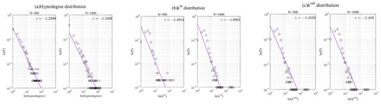
Figure 8. Structural characteristics of the network.

4.2. The Influence of Different Parameters on the Coupled Dynamics

This section investigates the impact of the parameters of the proposed $U{A}^H{A}^{P}U-SIS$ model on the scale of risk propagation through numerical experiments. All experimental results are obtained by simulating the model 50 times and taking the average. Initially, 2% of seed nodes are randomly selected as risk-infected nodes and nodes with a positive attitude toward risk. Bounded rational decision probability: ${\lambda }_P=0.4$, ${\lambda }_H=0.6$; bounded rational decision forgetting rate: ${\delta }_P=0.3$, ${\delta }_H=0.3$; risk preference: $\epsilon =0.8$; mass media reporting risk scale weakening factor: $\theta =0.5$; mass media information reinforcement effect: $\eta =4$; global perception ratio control factor: $K=0.4$; risk perception ability: $\alpha =0.6$; perception capacity decay factor: ${\Gamma }_U=0.1$, ${\Gamma }_H=0.6$; risk recovery rate: $\mu =0.3$; mean of the risk incubation period function: $v=2$. (The setting of parameter values is mainly referred to: [17,18,19,59,60]. Unless otherwise specified, all assumptions and parameters remain unchanged).

Firstly, the present paper employs the MMCA and Monte Carlo (MC) simulations to analyze the changing trends in the proportions of enterprises in different states during the risk propagation process based on the above parameter values. In the context of the MC simulation, ${\mathsf{\rho }}^{\mathrm{X}}={\displaystyle \frac{{\mathrm{N}}_{\mathrm{X}}}{\mathrm{N}}}$, $X=\left\{U,A^H,A^P,S,I\right\}$ where ${\mathrm{N}}_{\mathrm{X}}$ and $\mathrm{N}$ represent the number of X-state enterprises and total number of nodes, respectively. In the context of MMCA, ${\mathsf{\rho }}^{\mathrm{X}}=\sum _{\mathrm{i}=1}^{\mathrm{n}}{\displaystyle \frac{{\mathrm{P}}_{\mathrm{i}}^{\mathrm{x}}}{\mathrm{N}}}$, $X=\left\{U,A^H,A^P,S,I\right\}$, where ${\mathrm{P}}_{\mathrm{i}}^{\mathrm{X}}$ is the probability of node ${\mathrm{v}}_{\mathrm{i}}$ being in each state. As illustrated in Figure 9, the steady-state values of ${\rho }^I$, ${\rho }^{A^P}$, and ${\rho }^{A^H}$ were obtained through MMCA and MC simulations, respectively. The simulation results of the two methods show close agreement, indicating that MMCA is a highly effective theoretical framework for studying coupled dynamics in multiplexed networks. Consequently, all subsequent numerical simulations will utilize MMCA.

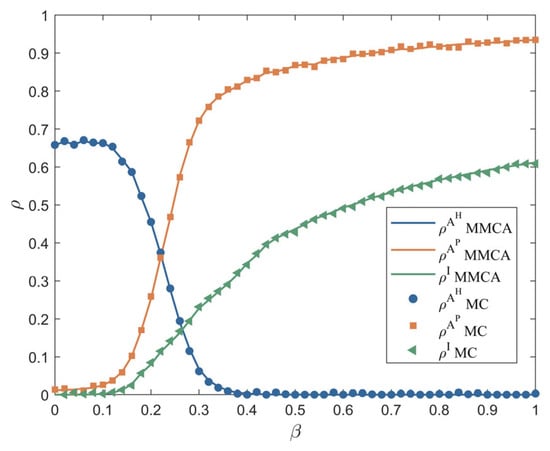
Figure 9. Comparison of experimental results obtained by MMCA and MC.

This paper compares the adaptive propagation model with the most commonly used global propagation based on the reaction process (RP) and local propagation based on the contact process (CP) in hypergraphs, with a basic infection probability of $\beta =0.6$. The results are shown in Figure 10a. At each time step, CP randomly selects only one hyperedge, RP propagates to all hyperedges, and AD propagates adaptively based on the weight values of the hyperedges. Therefore, CP has the smallest scale, RP has the largest scale, and AD falls between the two. Figure 10b illustrates the differences in the proportion of infected enterprises between the CP and AD models (CP-AD) and between the RP and AD models (RP-AD) at different $\beta$ values (from 0 to 1, with a step size of 0.05). The results clearly show that the difference between RP and AD first increases and then decreases with the increase in beta. The difference between CP and AD shows two trends of first increasing and then decreasing with the increase in beta, and the difference between CP and AD is smaller than that between RP and AD. The experimental results are consistent with previous studies [20], confirming the validity of the experimental results and further validating the applicability of the adaptive model.

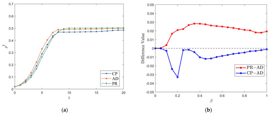
Figure 10. (a) Comparison of infection scale ${\rho }^I$ under different transmission models. (b) The differences in the ${\rho }^I$ between the CP and AD models (CP-AD) and between the RP and AD models (RP-AD) at different $\beta$.

In the following section, the focus is on an examination of the impact of other parameters on risk propagation in industrial symbiosis networks.

As illustrated in Figure 11, the effects of media reporting risk scale attenuation factor $\theta$ and risk propagation rate $\beta$ on the steady-state values of ${\rho }^I$, ${\rho }^{A^H}$, and ${\rho }^{A^P}$ are demonstrated. As the parameter $\theta$ increases, the risk scale ${\rho }^I$ undergoes a gradual decrease, the risk-positive attitude ${\rho }^{A^P}$ undergoes a gradual increase, and the risk hesitation state ${\rho }^{A^H}$ undergoes a gradual decrease. This is because the greater the risk scale attenuation factor $\theta$, the closer the risk scale and severity portrayed in mass media reports align with real-world risk levels. This enables symbiotic enterprises to rationally assess risk threats and implement appropriate risk prevention measures, thereby minimizing the probability of risk contagion. Furthermore, it can be observed that changes in $\theta$ do not affect the risk propagation threshold ${\beta }_c$, which is consistent with the conclusion of Theorem 1. This serves to further validate the accuracy of the proposed model.

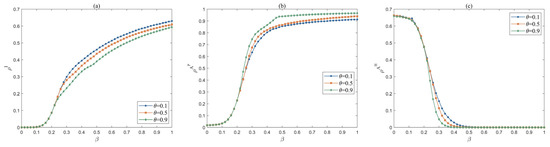
Figure 11. Effect of media reporting risk scale attenuation factor $\theta$ and risk propagation rate $\beta$ on density ${\rho }^I$, ${\rho }^{A^P}$, ${\rho }^{A^H}$. (a) The evolution trend of ${\rho }^I$ with increasing $\beta$ under different $\theta$. (b) The evolution trend of ${\rho }^{A^P}$ with increasing $\beta$ under different $\theta$. (c) The evolution trend of ${\rho }^{A^H}$ with increasing $\beta$ under different $\theta$.

Figure 12 shows the impact of bounded rational decision probabilities ${\lambda }_H$, ${\lambda }_P,$ and mass media reporting attenuation factor $\theta$ on ${\rho }^I$, ${\rho }^{A^P}$, and ${\rho }^{A^H}$ at the steady state. With basic risk propagation rate fixed $\beta$ at 0.3, ${\lambda }_H$ and ${\lambda }_P$ are varied from 0 to 1. As can be observed from Figure 12a, when ${\lambda }_H$ is fixed to any value in $\left[\mathrm{0,1}\right]$, the gradual increase in ${\lambda }_P$ leads to a decrease in ${\rho }^I$. This is because a larger ${\lambda }_P$ can trigger the rapid spread of positive risk attitudes (Figure 12c), while the spread of opposing hesitant risk attitudes is suppressed to some extent (Figure 12e). When ${\lambda }_P$ is large, the proportion of individuals with positive risk attitudes in the steady state is higher, leading to more companies adopting efficient self-protection measures to reduce the probability of being exposed to risk.

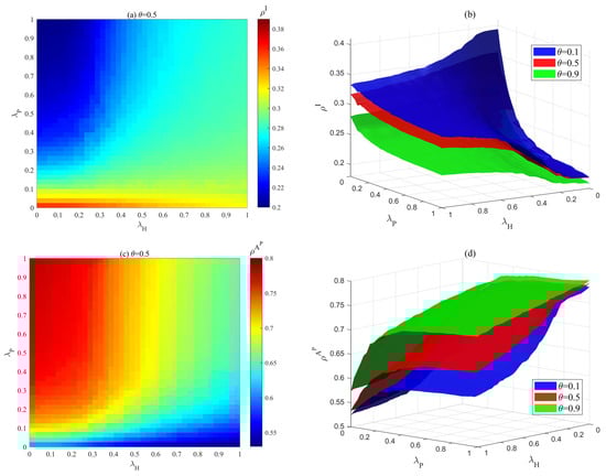
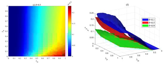
Figure 12. Effect of the impact of bounded rational decision probabilities ${\lambda }_H$, ${\lambda }_P$ and mass media reporting attenuation factor $\theta$ on ${\rho }^I$, ${\rho }^{A^P}$, ${\rho }^{A^H}$ at the steady state. (a) Dependence of ${\rho }^I$ on ${\lambda }_H$, ${\lambda }_P$ when $\theta =0.5$. (b) Dependence of ${\rho }^I$ on ${\lambda }_H$, ${\lambda }_P$ under different $\theta$. (c) Dependence of ${\rho }^{A^P}$ on ${\lambda }_H$, ${\lambda }_P$ when $\theta =0.5$. (d) Dependence of ${\rho }^{A^P}$ on ${\lambda }_H$, ${\lambda }_P$ under different $\theta$. (e) Dependence of ${\rho }^{A^H}$ on ${\lambda }_H$, ${\lambda }_P$ when $\theta =0.5$. (f) Dependence of ${\rho }^{A^H}$ on ${\lambda }_H$, ${\lambda }_P$ under different $\theta$.

On the other hand, as shown in Figure 12a, when the value of ${\lambda }_P$ is fixed, the effect of ${\lambda }_H$ on ${\rho }^I$ can be divided into two distinct cases. When ${\lambda }_P$ is less than 0.1, ${\rho }^I$ does not increase with an increase in ${\lambda }_H$ but instead shows a decreasing trend. There are two main reasons for this phenomenon. First, when ${\lambda }_P$ is small (${\lambda }_P<0.1$), the risk-positive attitude view is difficult to spread (Figure 12c), and risk propagation is almost unaffected by positive attitudes. Second, as ${\lambda }_H$ increases, an increasing number of firms in state $US$ receive risk information and shift to a risk-hesitant attitude (Figure 12e), but in the absence of effective positive information propagation, this phenomenon can still suppress risk propagation to some extent. However, when ${\lambda }_P>0.1$, an inversion phenomenon occurs, where the ${\rho }^I$ increases with increasing ${\lambda }_H$. In particular, this phenomenon becomes more pronounced when ${\lambda }_P$ is large, as a larger ${\lambda }_H$ creates a greater barrier to the spread of positive risk attitudes (Figure 12c). Overall, enhancing the probability of bounded rationality decision-making serves as a crucial means for effective risk control. This finding aligns with the prevailing principles of risk management within ISN, similar to the risk prevention and control mechanisms within the Kalundborg industrial symbiosis system, where enterprises establish effective risk buffering systems through information sharing and coordinated action.

In Figure 12b,d,f, the change trend of ${\rho }^I$, ${\rho }^{A^P}$, and ${\rho }^{A^H}$ with ${\lambda }_H$ and ${\lambda }_P$ is similar to that in Figure 12a,c,e. The difference lies in the fact that as $\theta$ increases, the risk scale ${\rho }^I$ gradually decreases, the proportion of companies with a positive attitude towards risk ${\rho }^{A^P}$ gradually increases, and the proportion of companies in a state of risk hesitation ${\rho }^{A^H}$ gradually decreases. This difference can be attributed to the impact of mass media and crowd effects on risk propagation. When more and more unaware and hesitant companies decide to take effective self-protection measures through the influence of mass media and crowd effects, the risk will be further controlled. This further validates the accuracy of Figure 11 and provides a reference framework for managing risks within real-world ISN.

Figure 13 shows the effects of bounded rational decision forgetting rates ${\delta }_H$, ${\delta }_P$ and mass media reporting attenuation factor $\theta$ on ${\rho }^I$, ${\rho }^{A^P}$, and ${\rho }^{A^H}$ at the steady state. With basic risk propagation rate fixed $\beta$ at 0.3, ${\delta }_H$ and ${\delta }_P$ are varied from 0 to 1. As illustrated in Figure 13a, when the parameter ${\delta }_H$ is assigned a value within the range $\left[\mathrm{0,1}\right]$, the subsequent rise in ${\delta }_P$ results in an increase in the density of ${\rho }^I$.This is because a larger ${\delta }_P$ causes the rapid disappearance of risk-positive attitudes (Figure 13c), resulting in a lower proportion of individuals with risk-positive attitudes in the steady state, making firms more exposed to risk.

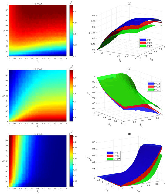
Figure 13. Effect of the bounded rational decision forgetting rates ${\delta }_H$, ${\delta }_P$ and mass media reporting attenuation factor $\theta$ on ${\rho }^I$, ${\rho }^{A^P}$, ${\rho }^{A^H}$ at the steady state. (a) Dependence of ${\rho }^I$ on ${\delta }_H$, ${\delta }_P$ when $\theta =0.5$. (b) Dependence of ${\rho }^I$ on ${\delta }_H$, ${\delta }_P$ under different $\theta$. (c) Dependence of ${\rho }^{A^P}$ on ${\delta }_H$, ${\delta }_P$ when $\theta =0.5$. (d) Dependence of ${\rho }^{A^P}$ on ${\delta }_H$, ${\delta }_P$ under different $\theta$. (e) Dependence of ${\rho }^{A^H}$ on ${\delta }_H$, ${\delta }_P$ when $\theta =0.5$. (f) Dependence of ${\rho }^{A^H}$ on ${\delta }_H$, ${\delta }_P$ under different $\theta$.

On the other hand, when the value of ${\delta }_P$ is fixed, the effect of ${\delta }_H$ on density ${\rho }^I$ exhibits two distinct scenarios. When ${\delta }_P<0.15$, the density ${\rho }^I$ decreases as ${\delta }_H$ increases. There are two main reasons for this. First, when ${\delta }_P<0.15$, a larger proportion of firms hold risk-positive attitudes and are less likely to forget them. By spreading these attitudes to neighboring firms, an increasing number of firms adopt efficient self-protection measures to address risks (Figure 13c). Second, when ${\delta }_P<0.15$, as ${\delta }_H$ increases, the reduction in the proportion of risk-hesitant firms is smaller compared to when ${\delta }_P$ is larger (Figure 13e), meaning this change does not affect risk propagation. However, when ${\delta }_P>0.15$, a reversal occurs, where density ${\rho }^I$ increases as ${\delta }_H$ increases.

In Figure 13b,d,f, the change trend of ${\rho }^I$, ${\rho }^{A^P}$, and ${\rho }^{A^H}$ with ${\delta }_H$ and ${\delta }_P$ is similar to that in Figure 13a,c,e. The difference lies in the fact that as $\theta$ increases, ${\rho }^I$ gradually decreases, ${\rho }^{A^P}$ gradually increases, and ${\rho }^{A^H}$ gradually decreases. This once again verifies the accuracy of Figure 11. This simulation outcome demonstrates intrinsic consistency with the risk coordination and prevention mechanisms observed in real-world ISN. Through efficient information exchange (corresponding to higher ${\lambda }_P$ and ${\lambda }_H$ values) and sustained maintenance of safety protocols (corresponding to lower ${\delta }_H$ and ${\delta }_P$ values), enterprises achieve systematic risk mitigation. The conclusions provide a theoretical framework for further understanding risk governance within actual ISN.

Figure 14 analyses the impact of risk perception ability $\alpha$ and risk propagation rate $\beta$ on ${\rho }^I$ at steady state, and shows the changes under different mass media reporting attenuation factors $\theta$ and different perception ability decay factors (${\mathit{\Gamma }}_U$, ${\mathit{\Gamma }}_H$). As shown in Figure 14a, as $\alpha$ increases, the scale of risk propagation decreases and the risk propagation threshold increases. This is because an enterprise’s risk perception capability determines its risk admission rate. As more enterprises develop higher risk perception capabilities, the risk admission rate decreases during risk propagation in ISN, making it difficult for risks to escalate within the system. Additionally, when the propagation rate $\beta$ is high, enhancing an enterprise’s risk perception capability can effectively control the scale of risk propagation. As shown in Figure 14b, for any given set of $\alpha$ and $\beta$, an increase in $\theta$ reduces the infection density ${\rho }^I$. Therefore, simultaneously enhancing firms’ risk perception capabilities and improving the timeliness and accuracy of mass media reporting can effectively suppress risk propagation.

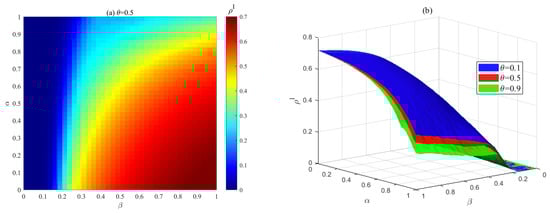
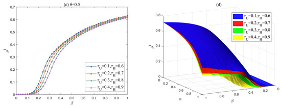
Figure 14. Effect of risk perception ability $\alpha$, risk propagation rate $\beta$, mass media reporting attenuation factor $\theta$, and risk perception decay factors (${\Gamma }_U$, ${\Gamma }_H$) on ${\rho }^I$ at the steady state. (a) Dependence of ${\rho }^I$ on $\alpha$, $\beta$ when $\theta =0.5$. (b) Dependence of ${\rho }^I$ on $\alpha$, $\beta$ under different $\theta$. (c) The evolution trend of ${\rho }^I$ with increasing $\beta$ under different (${\Gamma }_U$, ${\Gamma }_H$) when $\theta =0.5$. (d) Dependence of ${\rho }^I$ on $\alpha$, $\beta$ under different (${\Gamma }_U$, ${\Gamma }_H$) when $\theta =0.5$.

Figure 14c,d provide a detailed analysis of the impact of risk perception decay factors (${\mathit{\Gamma }}_U$, ${\mathit{\Gamma }}_H$) on the scale of risk propagation ${\rho }^I$, where ${\mathit{\Gamma }}_U$ and ${\mathit{\Gamma }}_H$ represent the perception decay coefficients for firms unaware of the risk and those maintaining a hesitant attitude toward the risk, respectively. As shown in Figure 14c, a decrease in ${\mathit{\Gamma }}_U$ and ${\mathit{\Gamma }}_H$ increases the scale of risk propagation and lowers the risk propagation threshold. This is primarily because enterprises’ risk perception capabilities have decreased, leading to an increase in the risk acceptance rate of susceptible enterprises, making them more prone to risk exposure. As shown in Figure 14c, as the infection probability $\beta$ increases, the influence of ${\mathit{\Gamma }}_U$ and ${\mathit{\Gamma }}_H$ on the risk scale ${\rho }^I$ diminishes. This is mainly because, under the influence of mass media and crowd effects, when $\beta$ increases, the rise in the number of infected individuals further promotes the spread of positive attitudes toward risk, thereby suppressing the proportion of companies that are unaware of risks or have hesitant attitudes toward risks to some extent, leading to a reduction in the effect of (${\mathit{\Gamma }}_U$, ${\mathit{\Gamma }}_H$). Figure 14d shows the impact of risk perception ability $\alpha$ and risk transmission rate $\beta$ on risk scale ${\rho }^I$ under different conditions of ${\mathit{\Gamma }}_U$ and ${\mathit{\Gamma }}_H$ when $\theta$ is fixed at 0.5, with the trend consistent with the above.

This finding aligns closely with the operational logic of mature industrial symbiosis systems. Taking the Kalundborg industrial symbiosis system as an example, its symbiotic enterprises have significantly enhanced their capacity for early identification and response to potential risks by establishing robust environmental monitoring and information-sharing mechanisms (equivalent to increasing $\alpha$). This has effectively prevented the diffusion and amplification of risks.

Figure 15 shows the impact of risk recovery capacity $\mu$ and risk propagation rate $\beta$ on ${\rho }^I$ at the stable state, with $\theta =0.5$. As can be observed from Figure 15a, ${\rho }^I$ decreases significantly as $\mu$ increases, and the risk propagation threshold increases significantly. Furthermore, when the propagation rate $\beta$ is high, enhancing a company’s risk resilience can effectively control the scale of risk propagation. A company’s risk resilience is a key indicator for measuring its ability to quickly resume normal operations and minimize losses following a risk event. As $\mu$ increases, companies can more efficiently reduce risk exposure time and optimize resource allocation, thereby significantly lowering the proportion of infected companies in the system. Figure 15b draws a phase diagram of the proportion of infected enterprises changing with risk recovery capacity $\mu$ and risk propagation rate $\beta$.

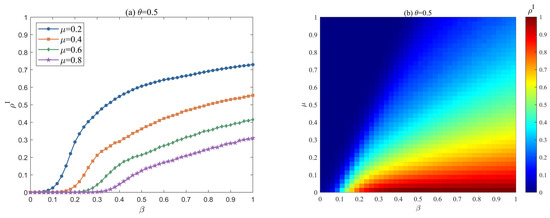
Figure 15. Effect of risk recovery capacity $\mu$ and risk propagation rate $\beta$ on ${\mathsf{\rho }}^{\mathrm{I}}$ at the steady state. (a) The evolution trend of ${\rho }^I$ with increasing $\beta$ under different $\mu$ when $\theta =0.5$. (b) Dependence of ${\rho }^I$ on $\mu$, $\beta$ when $\theta =0.5$.

Therefore, enhancing a company’s risk recovery capability not only reduces direct losses but also effectively suppresses risk diffusion within the symbiotic network, ultimately lowering the proportion of companies at risk of infection. Enterprises may systematically enhance their risk recovery capabilities and overall resilience through multi-dimensional strategies, including establishing redundant resources and backup systems, strengthening intelligent risk monitoring and response mechanisms, and improving risk adaptation capacity. This mechanism validates the core role of risk recovery capability within a company’s risk management system and provides a theoretical basis for optimizing risk response strategies.

5. Conclusions

The exchange of resources or by-products between enterprises in industrial symbiosis networks forms a coupled industrial ecological chain, promotes waste recycling, and balances the conflict between ecological protection and economic development. However, in the development of industrial symbiosis systems, various internal and external risk factors will inevitably lead to the spread of risk within the system. In this paper, we propose a coupled directed weighted multi-layer hypernetwork model to characterize the complex interaction between bounded rational decisions and risk propagation in enterprises under the influence of mass media and crowd effects.

This paper uses a time-varying adaptive hypernetwork model to simulate the formation process of bounded rational decisions made by enterprises in a symbiotic network and develops a risk propagation process that takes into account the degree of symbiotic dependence and k-shells. The constructed multi-layer hypernetwork evolution model has a scale-free characteristic and is very similar to a real network. This paper summarizes the role of mass media as a decision function and takes into account the crowd effect. In the process of enterprise risk state transformation, it innovatively introduces the latent period assumption of bounded rational decision-making and uses the Microscopic Markov Chain Approach to conduct theoretical analysis and numerical simulation of coupled dynamics. The proposed hypernetwork evolution model is theoretically derived with hyperdegree changes, combining theory and experiment to make the research more accurate and complete.

This study conducted an in-depth analysis of the risk diffusion mechanism in industrial symbiosis networks and drew the following important conclusions and management implications:

• Enhancing companies’ willingness to take proactive risk response measures is a key foundation. This requires the establishment of effective mechanisms and evaluation systems, as well as regular training and case reviews to reduce companies’ forgetfulness regarding proactive risk attitudes, ensuring that risk prevention awareness continues to play an effective role.
• Enhancing enterprises’ risk perception capabilities is the first line of defense against risk diffusion. This can be achieved by deploying intelligent monitoring systems, establishing risk warning models, and improving information sharing mechanisms, enabling enterprises to identify potential risks earlier and more accurately.
• Improving enterprises’ risk recovery capabilities is the core means of controlling the scope of risk impact. This requires establishing comprehensive emergency response plans, stockpiling critical resources, and optimizing organizational response processes to reduce risk resolution time and minimize losses.
• The timeliness and accuracy of mass media reporting play a significant regulatory role in risk propagation. A mechanism for information coordination between media and enterprises should be established to ensure the rapid dissemination of authoritative information and avoid the risk amplification effect caused by information distortion.

Overall, risk management in industrial symbiosis networks requires the establishment of a collaborative prevention and control system that organically combines technical means (such as big data analysis) with management innovation (such as cross-enterprise collaboration) to effectively enhance the overall resilience of the network. Future research can further explore the synergistic mechanisms of various elements in different industry contexts, as well as the in-depth application of digital technologies in risk prevention and control, to provide theoretical support and practical guidance for the construction of a safer industrial symbiosis system.

References

- Chertow, M.R. Industrial Symbiosis: Literature and Taxonomy. Annu. Rev. Energy Environ. 2000, 25, 313–337. [Google Scholar] [CrossRef]
- Lombardi, D.R.; Laybourn, P. Redefining Industrial Symbiosis: Crossing Academic–Practitioner Boundaries. J. Ind. Ecol. 2012, 16, 28–37. [Google Scholar] [CrossRef]
- Mantese, G.C.; Amaral, D.C. Agent-Based Simulation to Evaluate and Categorize Industrial Symbiosis Indicators. J. Clean. Prod. 2018, 186, 450–464. [Google Scholar] [CrossRef]
- Huang, B.; Yong, G.; Zhao, J.; Domenech, T.; Liu, Z.; Chiu, S.F.; McDowall, W.; Bleischwitz, R.; Liu, J.; Yao, Y. Review of the Development of China’s Eco-Industrial Park Standard System. Resour. Conserv. Recycl. 2019, 140, 137–144. [Google Scholar] [CrossRef]
- Liu, Z.; Adams, M.; Cote, R.P.; Geng, Y.; Ren, J.; Chen, Q.; Liu, W.; Zhu, X. Co-Benefits Accounting for the Implementation of Eco-Industrial Development Strategies in the Scale of Industrial Park Based on Emergy Analysis. Renew. Sustain. Energy Rev. 2018, 81, 1522–1529. [Google Scholar] [CrossRef]
- Wan, Z.; Su, Y.; Li, Z.; Zhang, X.; Zhang, Q.; Chen, J. Analysis of the Impact of Suez Canal Blockage on the Global Shipping Network. Ocean. Coast. Manag. 2023, 245, 106868. [Google Scholar] [CrossRef]
- Jacobsen, N.B. Industrial Symbiosis in Kalundborg, Denmark: A Quantitative Assessment of Economic and Environmental Aspects. J. Ind. Ecol. 2006, 10, 239–255. [Google Scholar] [CrossRef]
- Wang, Y.; Sun, Z.; Li, P.; Zhu, Z. Small World and Stability Analysis of Industrial Coupling Symbiosis Network of Ecological Industrial Park of Oil and Gas Resource Cities. Energy Explor. Exploit. 2021, 39, 853–868. [Google Scholar] [CrossRef]
- Gallese, V.; Mastrogiorgio, A.; Petracca, E.; Viale, R. Embodied Bounded Rationality. In Routledge Handbook of Bounded Rationality; Viale, R., Ed.; Routledge: London, UK, 2020; pp. 377–390. ISBN 978-1-315-65835-3. [Google Scholar]
- Petracca, E. Embodying Bounded Rationality: From Embodied Bounded Rationality to Embodied Rationality. Front. Psychol. 2021, 12, 710607. [Google Scholar] [CrossRef]
- Simon, H. Administrative Behavior; a Study of Decision-Making Processes in Administrative Organization; Macmillan: New York, NY, USA, 1947. [Google Scholar]
- Song, Y.; Yang, N.; Zhang, Y.; Wang, J. Suppressing Risk Propagation in R&D Networks: The Role of Government Intervention. Chin. Manag. Stud. 2019, 13, 1019–1043. [Google Scholar] [CrossRef]
- TAO, Y.; Morgan, D.; Evans, S. How Policies Influence the Implementation of Industrial Symbiosis: A Comparison between UK and China. Asian J. Manag. Sci. Appl. 2015, 2, 1. [Google Scholar] [CrossRef]
- Li, X.; Xiao, R. Analyzing Network Topological Characteristics of Eco-Industrial Parks from the Perspective of Resilience: A Case Study. Ecol. Indic. 2017, 74, 403–413. [Google Scholar] [CrossRef]
- Wang, D.; Li, J.; Wang, Y.; Wan, K.; Song, X.; Liu, Y. Comparing the Vulnerability of Different Coal Industrial Symbiosis Networks under Economic Fluctuations. J. Clean. Prod. 2017, 149, 636–652. [Google Scholar] [CrossRef]
- Wu, J.; Pu, G.; Ma, Q.; Qi, H.; Wang, R. Quantitative Environmental Risk Assessment for the Iron and Steel Industrial Symbiosis Network. J. Clean. Prod. 2017, 157, 106–117. [Google Scholar] [CrossRef]
- Shan, H.; Guo, Q.; Wei, J. The Impact of Disclosure of Risk Information on Risk Propagation in the Industrial Symbiosis Network. Environ. Sci. Pollut. Res. 2023, 30, 45986–46003. [Google Scholar] [CrossRef]
- Shan, H.; Liang, J.; Pi, W. The Impact of Risk Sharing on Risk Propagation in Multiplex Networks: A Dynamic Simulation on Industrial Symbiosis. Phys. Lett. A 2025, 529, 130110. [Google Scholar] [CrossRef]
- Yu, P.; Wang, P.; Wang, Z.; Wang, J. Supply Chain Risk Diffusion Model Considering Multi-Factor Influences under Hypernetwork Vision. Sustainability 2022, 14, 8420. [Google Scholar] [CrossRef]
- Pan, Q.; Wang, Z.; Wang, H.; Tang, J. Adaptive Dissemination Process in Weighted Hypergraphs. Expert. Syst. Appl. 2025, 268, 126340. [Google Scholar] [CrossRef]
- Kuznetsova, E.; Louhichi, R.; Zio, E.; Farel, R. Input-Output Inoperability Model for the Risk Analysis of Eco-Industrial Parks. J. Clean. Prod. 2017, 164, 779–792. [Google Scholar] [CrossRef]
- Zhang, X.; Chai, L. Structural Features and Evolutionary Mechanisms of Industrial Symbiosis Networks: Comparable Analyses of Two Different Cases. J. Clean. Prod. 2019, 213, 528–539. [Google Scholar] [CrossRef]
- Guo, J.-L.; Zhu, X.-Y.; Suo, Q.; Forrest, J. Non-Uniform Evolving Hypergraphs and Weighted Evolving Hypergraphs. Sci. Rep. 2016, 6, 36648. [Google Scholar] [CrossRef] [PubMed]
- Yook, S.H.; Jeong, H.; Barabási, A.-L.; Tu, Y. Weighted Evolving Networks. Phys. Rev. Lett. 2001, 86, 5835–5838. [Google Scholar] [CrossRef]
- Barrat, A.; Barthélemy, M.; Pastor-Satorras, R.; Vespignani, A. The Architecture of Complex Weighted Networks. Proc. Natl. Acad. Sci. USA 2004, 101, 3747–3752. [Google Scholar] [CrossRef]
- Soto, J.E.; Hernández, C.; Figueroa, M. JACC-FPGA: A Hardware Accelerator for Jaccard Similarity Estimation Using FPGAs in the Cloud. Future Gener. Comput. Syst. 2023, 138, 26–42. [Google Scholar] [CrossRef]
- Panda, A.; Paul, A. Genetic Divergence in French Bean Accessions. Legume Res. Int. J. 2025, 48, 376–384. [Google Scholar] [CrossRef]
- Cekic, E.; Pinar, E.; Pinar, M.; Dagcinar, A. Deep Learning-Assisted Segmentation and Classification of Brain Tumor Types on Magnetic Resonance and Surgical Microscope Images. World Neurosurg. 2024, 182, e196–e204. [Google Scholar] [CrossRef]
- Al-antari, M.A.; Al-masni, M.A.; Choi, M.-T.; Han, S.-M.; Kim, T.-S. A Fully Integrated Computer-Aided Diagnosis System for Digital X-Ray Mammograms via Deep Learning Detection, Segmentation, and Classification. Int. J. Med. Inform. 2018, 117, 44–54. [Google Scholar] [CrossRef] [PubMed]
- Nandini, Y.V.; Jaya Lakshmi, T.; Krishna Enduri, M.; Zairul Mazwan Jilani, M. Link Prediction in Complex Hyper-Networks Leveraging HyperCentrality. IEEE Access 2025, 13, 12239–12254. [Google Scholar] [CrossRef]
- Fu, L.; Ma, G.; Dou, Z.; Bai, Y.; Zhao, X. Local Balance and Information Aggregation: A Method for Identifying Central Influencers in Networks. Appl. Sci. 2025, 15, 2478. [Google Scholar] [CrossRef]
- Verma, K.L. Thermoelastic Symmetric and Antisymmetric Wave Modes with Trigonometric Functions in Laminated Plates. Int. J. Mech. Mater. Eng. 2014, 9, 4. [Google Scholar] [CrossRef]
- Wang, J.; Li, C.; Xia, C. Improved Centrality Indicators to Characterize the Nodal Spreading Capability in Complex Networks. Appl. Math. Comput. 2018, 334, 388–400. [Google Scholar] [CrossRef]
- Li, C.; Wang, L.; Sun, S.; Xia, C. Identification of Influential Spreaders Based on Classified Neighbors in Real-World Complex Networks. Appl. Math. Comput. 2018, 320, 512–523. [Google Scholar] [CrossRef]
- Barrat, A.; Barthélemy, M.; Vespignani, A. Modeling the Evolution of Weighted Networks. Phys. Rev. E 2004, 70, 066149. [Google Scholar] [CrossRef] [PubMed]
- Barabási, A.-L.; Albert, R. Emergence of Scaling in Random Networks. Science 1999, 286, 509–512. [Google Scholar] [CrossRef] [PubMed]
- Barrat, A.; Barthélemy, M.; Vespignani, A. Weighted Evolving Networks: Coupling Topology and Weight Dynamics. Phys. Rev. Lett. 2004, 92, 228701. [Google Scholar] [CrossRef] [PubMed]
- Hong, Z.; Zhou, H.; Wang, Z.; Yin, Q.; Liu, J. Coupled Propagation Dynamics of Information and Infectious Disease on Two-Layer Complex Networks with Simplices. Mathematics 2023, 11, 4904. [Google Scholar] [CrossRef]
- Wang, J.; Hu, R.; Xu, H. Coupled Simultaneous Evolution of Policy, Enterprise Innovation Awareness, and Technology Diffusion in Multiplex Networks. Mathematics 2024, 12, 2078. [Google Scholar] [CrossRef]
- Wang, J.; Wang, Z.; Yu, P.; Xu, Z. The Impact of Different Strategy Update Mechanisms on Information Dissemination under Hyper Network Vision. Commun. Nonlinear Sci. Numer. Simul. 2022, 113, 106585. [Google Scholar] [CrossRef]
- Xu, X.-J.; He, S.; Zhang, L.-J. Dynamics of the Threshold Model on Hypergraphs. Chaos Interdiscip. J. Nonlinear Sci. 2022, 32, 023125. [Google Scholar] [CrossRef]
- Xu, H.; Zhang, Y.; Jin, X.; Wang, J.; Wang, Z. The Evolution of Cooperation in Multigames with Uniform Random Hypergraphs. Mathematics 2023, 11, 2409. [Google Scholar] [CrossRef]
- Zhang, Z.; Mei, X.; Jiang, H.; Luo, X.; Xia, Y. Dynamical Analysis of Hyper-SIR Rumor Spreading Model. Appl. Math. Comput. 2023, 446, 127887. [Google Scholar] [CrossRef]
- Liu, S.; Zhao, D.; Sun, Y. Effects of Higher-Order Interactions and Impulsive Vaccination for Rumor Propagation. Chaos Interdiscip. J. Nonlinear Sci. 2024, 34, 123131. [Google Scholar] [CrossRef]
- Wu, Q.; Fu, X.; Zhang, H.; Small, M. Oscillations and phase transition in the mean infection rate of a finite population. Int. J. Mod. Phys. C 2010, 21, 1207–1215. [Google Scholar] [CrossRef]
- Loder, J.; Rinscheid, A.; Wüstenhagen, R. Why Do (Some) German Car Manufacturers Go Electric? The Role of Dynamic Capabilities and Cognitive Frames. Bus. Strat. Environ. 2024, 33, 1129–1143. [Google Scholar] [CrossRef]
- Wang, K.-L.; Wu, C.-X.; Ai, J.; Su, Z. Complex Network Centrality Method Based on Multi-Order K-Shell Vector. Acta Phys. Sin. 2019, 68, 196402. [Google Scholar] [CrossRef]
- Zhou, B.; Lv, Y.; Mao, Y.; Wang, J.; Yu, S.; Xuan, Q. The Robustness of Graph K-Shell Structure Under Adversarial Attacks. IEEE Trans. Circuits Syst. II Express Briefs 2022, 69, 1797–1801. [Google Scholar] [CrossRef]
- Choi, J.; Lim, J.; Bok, K.; Yoo, J. User Influence Determination using k-shell Decomposition in Social Networks. J. Korea Contents Assoc. 2022, 22, 46–54. [Google Scholar] [CrossRef]
- Kitsak, M.; Gallos, L.K.; Havlin, S.; Liljeros, F.; Muchnik, L.; Stanley, H.E.; Makse, H.A. Identification of Influential Spreaders in Complex Networks. Nat. Phys. 2010, 6, 888–893. [Google Scholar] [CrossRef]
- Pei, S.; Muchnik, L.; Andrade, J.; Zheng, Z.; Makse, H.A. Searching for Superspreaders of Information in Real-World Social Media. Sci. Rep. 2014, 4, 5547. [Google Scholar] [CrossRef] [PubMed]
- Jiang, J.; Dai, J. Time and Risk Perceptions Mediate the Causal Impact of Objective Delay on Delay Discounting: An Experimental Examination of the Implicit-Risk Hypothesis. Psychon. Bull. Rev. 2021, 28, 1399–1412. [Google Scholar] [CrossRef] [PubMed]
- Perrucci, D.V.; Aktaş, C.B.; Sorentino, J.; Akanbi, H.; Curabba, J. A Review of International Eco-Industrial Parks for Implementation Success in the United States. City Environ. Interact. 2022, 16, 100086. [Google Scholar] [CrossRef]
- Shen, A.-Z.; Guo, J.-L.; Suo, Q. Study of the Variable Growth Hypernetworks Influence on the Scaling Law. Chaos Solitons Fractals 2017, 97, 84–89. [Google Scholar] [CrossRef]
- Shen, A.-Z.; Guo, J.-L.; Wu, G.-L.; Jia, S.-W. The Agglomeration Phenomenon Influence on the Scaling Law of the Scientific Collaboration System. Chaos Solitons Fractals 2018, 114, 461–467. [Google Scholar] [CrossRef]
- Granell, C.; Gómez, S.; Arenas, A. Dynamical Interplay between Awareness and Epidemic Spreading in Multiplex Networks. Phys. Rev. Lett. 2013, 111, 128701. [Google Scholar] [CrossRef]
- Granell, C.; Gómez, S.; Arenas, A. Competing Spreading Processes on Multiplex Networks: Awareness and Epidemics. Phys. Rev. E 2014, 90, 012808. [Google Scholar] [CrossRef] [PubMed]
- Lv, S.; Wen, J.; Zhang, X. MPPINet: Multipath Permittivity Inversion Network for Tree Roots Ground-Penetrating Radar Image Recognition. IEEE Trans. Instrum. Meas. 2024, 73, 1–14. [Google Scholar] [CrossRef]
- Yu, P.; Wang, Z.; Sun, Y.; Wang, P. Risk Diffusion and Control under Uncertain Information Based on Hypernetwork. Mathematics 2022, 10, 4344. [Google Scholar] [CrossRef]
- Zhang, Z.; Zhu, K.; Wang, F. Indirect Information Propagation Model with Time-Delay Effect on Multiplex Networks. Chaos Solitons Fractals 2025, 192, 115936. [Google Scholar] [CrossRef]
Disclaimer/Publisher’s Note: The statements, opinions and data contained in all publications are solely those of the individual author(s) and contributor(s) and not of MDPI and/or the editor(s). MDPI and/or the editor(s) disclaim responsibility for any injury to people or property resulting from any ideas, methods, instructions or products referred to in the content. |
© 2025 by the authors. Licensee MDPI, Basel, Switzerland. This article is an open access article distributed under the terms and conditions of the Creative Commons Attribution (CC BY) license (https://creativecommons.org/licenses/by/4.0/).