Article

Variant Poisson Item Count Technique with Non-Compliance †

1
Department of Physics, Astronomy and Mathematics, University of Hertfordshire, Hatfield AL10 9AB, UK
2
School of Mathematical Sciences, South China Normal University, Guangzhou 510631, China
3
Cheers Psychological Consultancy Services, Hong Kong, China
4
Department of Statistics and Data Science, Southern University of Science and Technology, Shenzhen 518055, China
*
Author to whom correspondence should be addressed.
This paper is an extension version of our paper published in 33rd International Workshop of Statistical Modelling, Bristol, UK, 16–20 July 2018; pp. 161–164.
Mathematics 2025, 13(18), 2973; https://doi.org/10.3390/math13182973
Submission received: 23 July 2025 / Revised: 3 September 2025 / Accepted: 5 September 2025 / Published: 14 September 2025
(This article belongs to the Section D1: Probability and Statistics)

Abstract

In this article, we propose a variant Poisson item count technique (VPICT) that explicitly accounts for respondent non-compliance in surveys involving sensitive questions. Unlike the existing Poisson item count technique (PICT), the proposed VPICT (i) replaces the sensitive item with a triangular model that combines the sensitive and an additional non-sensitive item; (ii) utilizes data from both control and treatment groups to estimate the prevalence of the sensitive characteristic, thereby improving the accuracy and efficiency of parameter estimation; and (iii) limits the occurrence of the floor effect to cases where the respondent neither possesses the sensitive characteristic nor meets the non-sensitive condition, thus protecting a subset of respondents from privacy breaches. The method introduces a mechanism to estimate the rate of non-compliance alongside the sensitive trait, enhancing overall estimation reliability. We present the complete methodological framework, including survey design, parameter estimation via the EM algorithm, and hypothesis testing procedures. Extensive simulation studies are conducted to evaluate performance under various settings. The practical utility of the proposed approach is demonstrated through an application to real-world survey data on illegal drug use among high school students.

1. Introduction

Accurate data collection and analysis in surveys involving sensitive or stigmatizing behaviors remain a persistent challenge in social science, public health, and behavioral research. When participants are asked directly about private or potentially incriminating information—such as illicit behavior, socially undesirable actions, or taboo personal experiences—they often respond in ways that align with perceived social norms rather than disclosing the truth. This response bias seriously compromises the validity of prevalence estimates and can distort the results of any subsequent analysis. For instance, van der Heijden et al. [1] reported that only 19% of respondents who had committed welfare or unemployment benefit fraud admitted doing so when asked directly, despite confidentiality assurances. Such reluctance to reveal sensitive truths reflects the deeply rooted social pressures and privacy concerns that respondents face, leading to substantial underreporting and biased findings.
To mitigate this issue and enhance the reliability of survey responses, a number of indirect questioning techniques have been developed. Among the most established is the randomized response (RR) technique, introduced by Warner [2]. This method involves using a randomizing device, such as a coin flip or a random number generator, to determine how a respondent should answer a question—either truthfully or following a pre-specified rule—thereby introducing a controlled level of uncertainty that protects individual privacy while still allowing for unbiased population-level estimates. Extensions and refinements of the RR method have been widely explored in the literature, offering sophisticated mechanisms for maintaining anonymity while improving response accuracy.
In more recent years, non-randomized response (NRR) techniques have gained attention as viable alternatives that avoid the use of randomizing devices altogether. Instead, these designs incorporate a non-sensitive question alongside a sensitive one in a strategic manner, such that the response to the composite query does not reveal which component triggered the answer. This innovation allows for the preservation of respondent confidentiality while reducing administrative complexity. Yu et al. [3] provide an excellent overview of NRR techniques, highlighting their advantages and limitations in practical settings.
Another influential method in this domain is the item count technique (ICT) [4], also known as the unmatched count technique or block total response method [5]. Under ICT, participants are randomly assigned to either a control group or a treatment group. Both groups receive a list of innocuous yes/no questions, but the treatment group’s list includes one additional sensitive question. Rather than answering each question individually, respondents report only the total number of “yes” answers. The difference in mean totals between the two groups is then used to estimate the prevalence of the sensitive attribute. ICT offers several advantages: it is simple to administer, easy to explain to respondents, and effectively conceals individual responses to sensitive items.
Despite its intuitive appeal and growing popularity, ICT has several important drawbacks [6]. One of the most significant is the presence of ceiling and floor effects. If a respondent in the treatment group answers “yes” to all questions, they may be identifiable as possessing the sensitive attribute, potentially compromising anonymity. Similarly, if a respondent in either group answers “no” to all questions, it may be inferred that they do not possess the sensitive attribute. These vulnerabilities can discourage respondents from answering truthfully and may even lead to non-compliance, particularly among those with the sensitive trait who fear disclosure. Additionally, ICT lacks standard guidelines for determining the number and composition of non-sensitive items, and it often assumes independence and known prevalence of these items—assumptions that may not hold in real-world applications.
Moreover, like many other indirect questioning techniques, ICT and its variants generally assume that respondents comply fully with the survey design and answer honestly. This so-called “no-liar” assumption is often unrealistic. Even under RR conditions, it was reported that fewer than 52% of those who admitted to fraud when protected by randomization were truthful, indicating a significant level of residual dishonesty [1]. Wu and Tang [7] showed that failure to model non-compliance in NRR contexts could lead to substantial underestimation of the true prevalence of sensitive behaviors, such as premarital sex. Recognizing the seriousness of this issue, a growing body of research has attempted to model deliberate underreporting as a form of self-protective behavior. For example, Böckenholt and van der Heijden [8] proposed a mixture model that accounts for non-cooperative respondents in RR surveys. Similarly, Cruyff et al. [9] introduced a log-linear randomized response model capable of measuring self-protective tendencies. In the NRR setting, Wu and Tang [7] incorporated an explicit non-compliance parameter to improve estimation accuracy.
The Poisson item count technique (denoted as PICT) was recently introduced as a variant of ICT to address the ceiling effect by assuming that the total number of “yes” answers follows a Poisson distribution [10]. This refinement enhances privacy protection, particularly for respondents with the sensitive attribute. However, the PICT still does not account for the floor effect and continues to rely on the assumption that all respondents comply with the survey instructions. In this setting, a response of zero can unambiguously identify a participant as not having the sensitive trait, which may prompt those who do possess the attribute to falsely report a zero in order to avoid exposure. Consequently, deliberate underreporting persists, and the resulting parameter estimates are biased and unreliable.
To address these challenges, we propose a novel method called the variant Poisson item count technique (denoted as VPICT). Our method extends the existing PICT by explicitly modeling respondent non-compliance. Specifically, we assume that individuals with the sensitive characteristic may choose to falsely report zero—denying their attribute—due to feelings of guilt, fear, or a desire to conform to social expectations. We introduce a non-compliance parameter, denoted by θ , which represents the probability that a respondent with the sensitive trait will misreport. Conversely, respondents who do not possess the sensitive attribute are assumed to comply with the survey protocol and respond truthfully. This modeling framework allows for more accurate estimation of the true prevalence of sensitive attributes and provides valuable insights into the extent of self-protective behavior among respondents.
The structure of this paper is as follows. In Section 2, we present the survey design and derive the maximum likelihood estimators for the model parameters. Section 3 develops hypothesis tests for both the target prevalence and the non-compliance rate. Section 4 reports the results of simulation studies designed to evaluate the statistical performance of our proposed method under various scenarios. In Section 5, we apply the VPICT to real-world survey data concerning illegal drug use among high school students to illustrate its practical utility. Finally, Section 6 offers concluding remarks and discusses potential avenues for further research.

2. Variant Poisson Item Count Techniques with Non-Compliance

In this section, we will propose a variant of the existing Poisson ICT (i.e., VPICT) which allows the estimation of the target proportion in the presence of the non-compliance assumption. Point as well as confidence interval estimation will be developed.

2.1. Survey Design

Assume that the sensitive question of interest is binary (e.g., whether the respondent has ever used illegal drugs in the past 30 days), and our objective is to estimate the prevalence of this sensitive characteristic in the presence of non-compliance. To this end, let n 1 and n 2 respondents be randomly assigned to the first and second groups, respectively, where n = n 1 + n 2 . All n respondents are instructed to answer the following non-sensitive question:
(1) How many times did you travel abroad last year?
In addition, respondents in the first group ( n 1 individuals) are required to answer:
(2) If you were born between January and March and you have never used illegal drugs in the past 30 days (i.e., you do not possess the sensitive characteristic), answer 0; otherwise, answer 1.
Similarly, respondents in the second group ( n 2 individuals) are instructed:
(2) If you were born between April and December and you have never used illegal drugs in the past 30 days, answer 0; otherwise, answer 1.
Finally, all respondents are asked to report only the sum of their answers to questions (1) and (2). For example, a respondent born in January who has never used illegal drugs in the past 30 days and traveled abroad four times last year would report a total of 4 in the first group and 5 in the second group.
In this design, the response to the first question (i.e., the number of trips abroad) is modeled as a count variable X 0 , 1 , , assumed to follow a Poisson distribution with parameter λ . In the second question, the non-sensitive binary variable (birth month), denoted by W, is assumed independent of the sensitive binary variable Z (whether the respondent has ever used illegal drugs in the past 30 days). Specifically, W = 1 indicates birth between April and December, and W = 0 otherwise. The probability p = Pr ( W = 1 ) is assumed known.
Let Z denote the sensitive characteristic, where Z = 1 if the respondent has used illegal drugs in the past 30 days and Z = 0 otherwise. We assume Z Bernoulli ( π ) , where π = Pr ( Z = 1 ) is the unknown parameter of interest. However, some respondents may provide a dishonest answer of 0 with probability θ , in order to conceal the sensitive behavior and project a socially desirable image.
To account for this non-compliance, we introduce a binary variable U, where U = 1 indicates non-compliance. We let Q ( i ) denote the response to the second question for group i, where i = 1 corresponds to the first group and i = 2 to the second group. Note that U and Z are not independent. Specifically, θ = Pr ( U = 1 Z = 1 ) . Here, we assume a respondent will always (i) comply with the design if (s)he does not possess the sensitive characteristic (i.e., Pr ( U = 1 Z = 0 ) = 0 ), and (ii) choose the safe answer if (s)he does not comply with the design (i.e., Pr ( Q ( i ) = 0 U = 1 ) = 1 , i = 1 , 2 ). Therefore, a respondent born in January who has used illegal drugs in the past 30 days, traveled abroad four times last year, and belonged to the first group would report a total of 5 if he complied with the instruction, or 4 if he refused to comply with the instruction.
It is noteworthy that Wu et al. [11] proposed another PICT which accounts for non-compliance (denoted as PICTNC). However, our proposed VPICT differs from PICTNC (and also PICT) in three key aspects. First, while PICTNC incorporates only the Poisson count question (i.e., X) and the sensitive question (i.e., Z), the VPICT additionally introduces a non-sensitive question (i.e., W or its complement), which is combined with the sensitive question. This modification is indeed a combination of the PICT and the triangular model in [3]. That is, the proposed method uses the PICT’s way of asking respondents the answer to the non-sensitive Poisson item and adds the idea of the triangular model of combining sensitive and non-sensitive items. Second, in PICTNC, the control group is asked to respond only to the Poisson count question (X), whereas the treatment group is required to report the sum of the Poisson count and the sensitive question ( X + Z ). Consequently, the control group only contributes to the estimation of the Poisson parameter ( λ ), resulting in a less efficient estimation of the prevalence of the sensitive characteristic ( π ). In contrast, VPICT utilizes the sensitive question in the first and second groups, allowing all respondents to contribute information for the estimation of π . This integrated design improves the efficiency of the estimator for π . Third, under the PICT(NC), if a respondent in the treatment group’s truthful answers to all of the items are negative, then the final answer is zero, which reveals the non-possession of the sensitive characteristic (i.e., floor effect). Under VPICT, the floor effect occurs only when the respondent does not have the sensitive characteristic AND fulfils the non-sensitive condition. As a result, a portion of the respondents who do not possess the sensitive characteristic will be protected from the floor effect.

2.2. Point Estimate

Let the observed data in the first and second groups be y 1 ( 1 ) , , y n 1 ( 1 ) and y 1 ( 2 ) , , y n 2 ( 2 ) , respectively. It is easy to show that (see Appendix A)
Y ( 1 ) = X + [ 1 ( 1 Z ) ( 1 W ) ] ( 1 U ) ,   and Y ( 2 ) = X + [ 1 ( 1 Z ) W ] ( 1 U )
We first derive the method of moment estimate (MOME) (denoted as π ^ M O M ) for π . For this purpose, we note that (see Appendix A)
E ( Y ( 1 ) ) = λ + 1 [ ( 1 p ) ( 1 π ) + π θ ] ,   and E ( Y ( 2 ) ) = λ + 1 [ p ( 1 π ) + π θ ] .
It is easy to see that
π ^ M O M = 1 y ¯ ( 1 ) y ¯ ( 2 ) 2 p 1 .
However, the method of moment estimate may occasionally yield values outside the admissible interval [ 0 , 1 ] if y ¯ ( 2 ) y ¯ ( 1 ) 1 2 p < 0 or y ¯ ( 2 ) y ¯ ( 1 ) 1 2 p > 1 . This often occurs especially when the true parameter is close to its boundaries (i.e., 0 or 1).
To overcome the above issue, we consider the maximum likelihood estimate (MLE). For this purpose, we assume the first m 1 and m 2 observations in the first and second groups are 0, respectively, and notice that the observed likelihood function is
L ( π , θ , λ | Y obs ) = e λ ( 1 p ) ( 1 π ) + π θ m 1 × e λ p ( 1 π ) + π θ m 2 × i = m 1 + 1 n 1 e λ λ y i ( 1 ) y i ( 1 ) ! ( 1 p ) ( 1 π ) + π θ + e λ λ y i ( 1 ) 1 ( y i ( 1 ) 1 ) ! p ( 1 π ) + π ( 1 θ ) × i = m 2 + 1 n 2 e λ λ y i ( 2 ) y i ( 2 ) ! p ( 1 π ) + π θ + e λ λ y i ( 2 ) 1 ( y i ( 2 ) 1 ) ! ( 1 p ) ( 1 π ) + π ( 1 θ ) .
It is easy to observe that there is no closed-form solution for the target parameter π . Here, we will develop the EM algorithm to obtain the MLEs. First, we introduce the missing data Y mis = { { x j ( 1 ) , z j ( 1 ) , u j ( 1 ) } j = 1 n 1 ; { x j ( 2 ) , z j ( 2 ) , u j ( 2 ) } j = 1 n 2 } with { x j ( 1 ) } , { x j ( 2 ) } being the answers to the counting question in the first and second group respectively, { z j ( 1 ) } and { z j ( 2 ) } being the answers to the sensitive question in the first and second group respectively, and { u j ( 1 ) } and { u j ( 2 ) } being the non-compliance variables.
The likelihood function based on the complete observation is:
L ( π , θ , λ | Y com ) = i = 1 n 1 e λ λ x i ( 1 ) x i ( 1 ) ! ( π θ ) z i ( 1 ) u i ( 1 ) ( 1 π ) 1 z i ( 1 ) [ π ( 1 θ ) ] z i ( 1 ) ( 1 u i ( 1 ) ) × i = 1 n 2 e λ λ x i ( 2 ) x i ( 2 ) ! ( π θ ) z i ( 2 ) u i ( 2 ) ( 1 π ) 1 z i ( 2 ) [ π ( 1 θ ) ] z i ( 2 ) ( 1 u i ( 2 ) )
and the log-likelihood is then
= c + i = 1 n 1 [ λ + x i ( 1 ) log λ + z i ( 1 ) log π + ( 1 z i ( 1 ) ) log ( 1 π ) + z i ( 1 ) u i ( 1 ) log ( θ ) + z i ( 1 ) ( 1 u i ( 1 ) ) log ( 1 θ ) ] + i = 1 n 2 [ λ + x i ( 2 ) log λ + z i ( 2 ) log π + ( 1 z i ( 2 ) ) log ( 1 π ) + z i ( 2 ) u i ( 2 ) log ( θ ) + z i ( 2 ) ( 1 u i ( 2 ) ) log ( 1 θ ) ] ,
where c is a constant.
The M step calculates the MLEs based on the complete likelihood and yields
π = i = 1 n 1 z i ( 1 ) + i = 1 n 2 z i ( 2 ) n 1 + n 2 , θ = i = 1 n 1 z i ( 1 ) u i ( 1 ) + i = 1 n 2 z i ( 2 ) u i ( 2 ) i = 1 n 1 z i ( 1 ) + i = 1 n 2 z i ( 2 ) , and λ = i = 1 n 1 x i ( 1 ) + i = 1 n 2 x i ( 2 ) n 1 + n 2 .
The E step finds the conditional expectation and gives
E ( X i ( 1 ) | y i ( 1 ) ) = y i ( 1 ) ( y i ( 1 ) 1 ) π ( 1 θ ) + p ( 1 π ) + y i ( 1 ) λ π θ + ( 1 p ) ( 1 π ) y i ( 1 ) π ( 1 θ ) + p ( 1 π ) + λ π θ + ( 1 p ) ( 1 π ) , E ( X i ( 2 ) | y i ( 2 ) ) = y i ( 2 ) ( y i ( 2 ) 1 ) π ( 1 θ ) + ( 1 p ) ( 1 π ) + y i ( 2 ) λ π θ + p ( 1 π ) y i ( 2 ) π ( 1 θ ) + ( 1 p ) ( 1 π ) + λ π θ + p ( 1 π ) , E ( Z i ( 1 ) | y i ( 1 ) ) = π y i ( 1 ) ( 1 θ ) + λ θ y i ( 1 ) π ( 1 θ ) + p ( 1 π ) + λ π θ + ( 1 p ) ( 1 π ) , E ( Z i ( 2 ) | y i ( 2 ) ) = π y i ( 2 ) ( 1 θ ) + λ θ y i ( 2 ) π ( 1 θ ) + ( 1 p ) ( 1 π ) + λ π θ + p ( 1 π ) , E ( U i ( 1 ) | y i ( 1 ) ) = π λ θ y i ( 1 ) π ( 1 θ ) + p ( 1 π ) + λ π θ + ( 1 p ) ( 1 π ) , and E ( U i ( 2 ) | y i ( 2 ) ) = π λ θ y i ( 2 ) π ( 1 θ ) + ( 1 p ) ( 1 π ) + λ π θ + p ( 1 π ) .
The derivations of the E and M steps are presented in Appendix B. Here, we use the MOME as the initial value and repeat the E and M steps until the estimates converge.

2.3. Confidence Interval Estimate

Let γ ^ = ( π ^ , θ ^ , λ ^ ) be the MLEs of γ = ( π , θ , λ ) obtained from the EM algorithm. Usually, we can construct the Wald-type confidence intervals (CIs) of the parameters using the square root of the diagonal elements of the inverse Fisher information, evaluated at γ = γ ^ . It should be noted that both Bernoulli parameters (i.e., π and θ ) should lie between 0 and 1. In practice, the upper (or lower) bounds of these Wald CIs may be greater (or less) than 1 (or 0), resulting in invalid CIs. Alternatively, we employ the bootstrap method to construct the bootstrap CI for any arbitrary function of γ , denoted by ϑ = h( γ ). Briefly, based on the obtained MLEs γ ^ = ( π ^ , θ ^ , λ ^ ) , we can independently generate y 1 ( 1 ) , , y n 1 ( 1 ) ; y 1 ( 2 ) , , y n 2 ( 2 ) according to the stochastic representation in (1). Having obtained the observed data, we can calculate the parameter estimates γ ^ * and obtain the bootstrap replication ϑ ^ * = h( γ * ). Independently repeating this process G times, we obtain G replications { ϑ ^ g * } g = 1 G . The bootstrap CI for ϑ can be constructed by
[ ϑ L , ϑ U ]
where L and U are the 100( α /2) and 100(1 − α /2) percentiles of { ϑ ^ g * } g = 1 G , respectively.

3. Hypothesis Testing

3.1. Hypothesis Testing of Sensitive Proportion

Suppose that we are interested in testing the following hypotheses
H 0 : π = π 0 vs . H 1 : π π 0
where π 0 is a pre-specified number. For the null hypothesis H 0 specified above, the likelihood ratio test (LRT) statistic is given by
T 1 = 2 [ ( π = π 0 , λ ^ 0 , θ ^ 0 | Y o b s ) ( π ^ , λ ^ , θ ^ | Y o b s ) ] ,
where π ^ , λ ^ , θ ^ are the unconstrained MLEs being calculated by (3) and (4), and λ ^ 0 and θ ^ 0 are the constrained MLEs under the null hypothesis H 0 : π = π 0 . The following EM algorithm can be employed to find the constrained MLEs λ ^ 0 and θ ^ 0 under H 0 .
The M step is to calculate the constrained MLEs:
λ = i = 1 n 1 x i ( 1 ) + i = 1 n 2 x i ( 2 ) n 1 + n 2 , and θ = i = 1 n 1 z i ( 1 ) u i ( 1 ) + i = 1 n 2 z i ( 2 ) u i ( 2 ) i = 1 n 1 z i ( 1 ) + i = 1 n 2 z i ( 2 ) .
The E step is to find the conditional expectation:
E ( X i ( 1 ) | y i ( 1 ) ) = y i ( 1 ) ( y i ( 1 ) 1 ) π 0 ( 1 θ ) + p ( 1 π 0 ) + y i ( 1 ) λ π 0 θ + ( 1 p ) ( 1 π 0 ) y i ( 1 ) π 0 ( 1 θ ) + p ( 1 π 0 ) + λ π 0 θ + ( 1 p ) ( 1 π 0 ) , E ( X i ( 2 ) | y i ( 2 ) ) = y i ( 2 ) ( y i ( 2 ) 1 ) π 0 ( 1 θ ) + ( 1 p ) ( 1 π 0 ) + y i ( 2 ) λ π 0 θ + p ( 1 π 0 ) y i ( 2 ) π 0 ( 1 θ ) + ( 1 p ) ( 1 π 0 ) + λ π 0 θ + p ( 1 π 0 ) , E ( U i ( 1 ) | y i ( 1 ) ) = π 0 λ θ y i ( 1 ) π 0 ( 1 θ ) + p ( 1 π 0 ) + λ π 0 θ + ( 1 p ) ( 1 π 0 ) , E ( U i ( 2 ) | y i ( 2 ) ) = π 0 λ θ y i ( 2 ) π 0 ( 1 θ ) + ( 1 p ) ( 1 π 0 ) + λ π 0 θ + p ( 1 π 0 ) , E ( Z i ( 1 ) | y i ( 1 ) ) = n 1 π 0 ,   and E ( Z i ( 2 ) | y i ( 2 ) ) = n 2 π 0 .
Here, the moment estimate is employed to be the initial value, and we repeat the E step and M step until the estimates are convergent. Let χ 2 ( 1 ) be the chi-square random variable with one degree of freedom and t 1 be the observed value of T 1 . Under the null hypothesis, T 1 is asymptotically chi-squared distributed with one degree of freedom. Hence, the null hypothesis is rejected if the p-value p 1 (= Pr ( χ 2 ( 1 ) > t 1 | H 0 ) ) is less than the prespecified significance level α .

3.2. Hypothesis Testing of Non-Compliance Parameter

To check whether the respondents comply with the design, we test whether the non-compliance parameter is 0 or not. That is, we consider the following hypotheses
H 0 : θ = 0 vs . H 1 : θ > 0 .
Again, we consider the following likelihood ratio test
T 2 = 2 [ ( π ^ 0 , λ ^ 0 , θ = 0 | Y o b s ) ( π ^ , λ ^ , θ ^ | Y o b s ) ] ,
where π ^ 0 , λ ^ 0 are the constrained MLEs under the null hypothesis H 0 , and π ^ , λ ^ , and θ ^ are unconstrained MLEs.
It is noteworthy that the null hypothesis H 0 corresponds to the parameter of interest (i.e., θ ) lying on the boundary of the parameter space (i.e., 0). As pointed out by Self and Liang [12] and Feng and McCulloch [13], the standard asymptotic theory suggesting that under H 0 T 2 is chi-squared distributed may not be appropriate. Instead, it is suggested that the appropriate reference null distribution for T 2 is a mixture of χ 2 distributions. Specifically, the appropriate reference distribution under H 0 is an equal mixture of a χ 2 ( 0 ) (i.e., a constant at zero) and a χ 2 ( 1 ) with the corresponding p-value being given by [14,15]
p 2 = Pr ( T 2 > t 2 | H 0 ) = 1 2 Pr ( χ 2 ( 1 ) > t 2 ) ,
where t 2 is the observed value of T 2 . Again, the hypothesis is rejected if p 2 is less than the prespecified significance level α .

4. Simulation Studies

In this section, all the simulations are performed using R Version 4.4.2.

4.1. Parameter and Confidence Interval Estimates

To evaluate the performance of the proposed point and confidence interval estimates, we consider two non-compliance cases: θ = 0.3 and θ = 0.4 . In surveys with sensitive questions, the proportion of such individuals is generally small. For both cases, we therefore consider π = ( 0.05 , 0.1 , 0.2 , 0.3 , 0.4 ) , p = 0.2 , and λ = 2. For each configuration, we generate { y j ( 1 ) , y j ( 2 ) } j = 1 n according to (1) with n = 1000 , and calculate the MLEs via the EM algorithm (3) and (4) and the 95% bootstrap CIs with G = 1000. Here, we independently repeat this process 1000 times. The corresponding average MLE and average width and average coverage probability of the bootstrap CIs are reported in Table 1 for θ = 0.3 and Table 2 for θ = 0.4 .
It is interesting to note that our proposed VPICT (with non-compliance) produces satisfactory point estimates and confidence interval estimates when the sensitive proportion lies away from boundary values (i.e., 0 and 1). When π = 0.05 , for example, larger estimate biases, wider confidence interval widths, and smaller coverage probabilities are observed. For π = 0.30 , all biases, confidence interval widths, and coverage probabilities substantially improve. On the contrary, estimation of λ is robust for different values of π and θ .

4.2. Hypothesis Testing

In this section, we conduct simulation studies to assess the performance of the likelihood ratio test for the hypothesis regarding the non-compliance parameter (i.e., T 2 ). First, we investigate the performance of its type I error rate. For this purpose, we set λ = 2 , p = 0.2 and θ = 0 . To examine the effect of the value of π , we set n = 1000 and π = 0.05 , 0.1 , 0.2 , 0.3 , 0.4 . For each parameter configuration, we generate { y j ( 1 ) , y j ( 2 ) } j = 1 n according to Equation (1). The test statistic T 2 is then calculated according to Equation ( 7 ) , and the null hypothesis is rejected if p 2 is less than the pre-specified value α = 0.05 . This process is independently repeated 1000 times, and the proportion of rejections is plotted as the simulated type I error rate in Figure 1. It is clear that the empirical type I error rates fluctuate around the pre-specified nominal level of α being 0.05 .
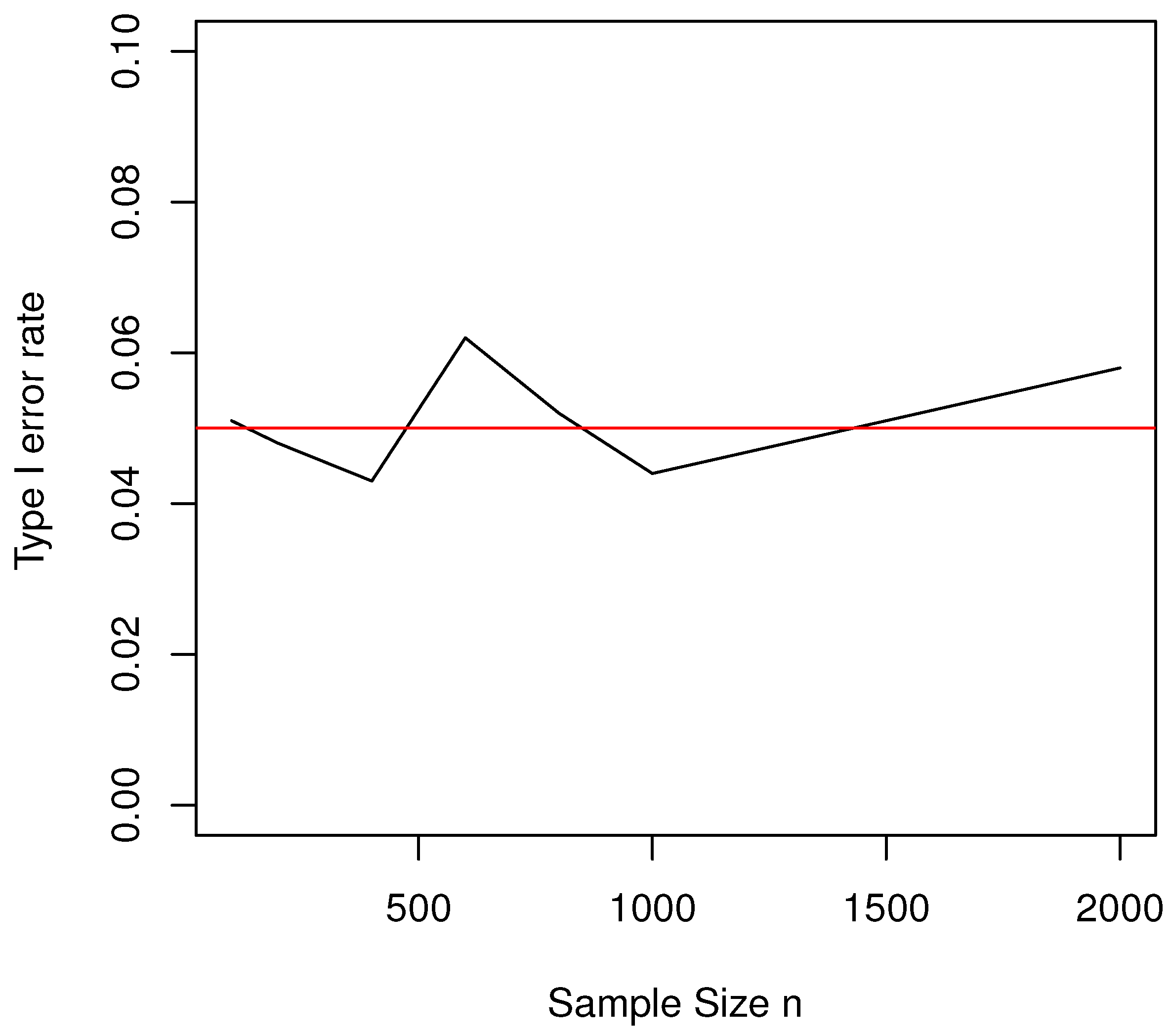
To investigate the influence of sample size on the type I error rate, we set π = 0.2 , θ = 0 and n = 100 , 200 , 400 , 600 , 800 , 1000 , 2000 . Similar to the previous simulation study, the empirical type I error rates are computed based on 1000 repetitions for each configuration. The results are plotted in Figure 2. It is clear that our proposed test is robust for different sample sizes n, even for small sample sizes (e.g., n = 100 ). The simulation results from Figure 1 and Figure 2 show that our proposed likelihood ratio test T 2 is a valid test and behaves satisfactorily in the sense that its empirical type I error rate is close to the nominal level (i.e., α = 0.05 ) for different sensitive proportions (i.e., π ) and sample sizes (i.e., n).
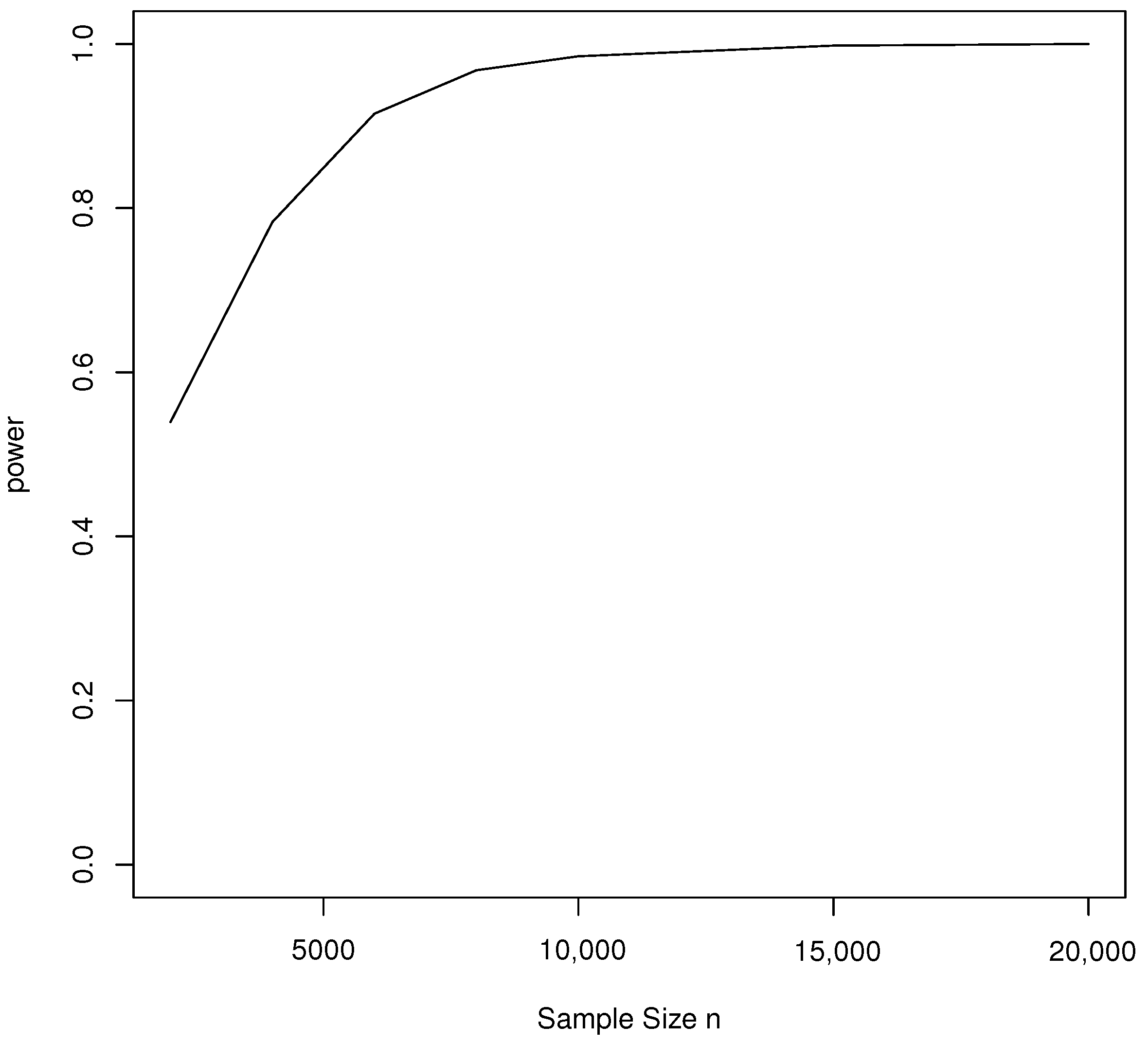
Finally, we investigate the power of the proposed T 2 test for the non-compliance parameter θ when π = 0.2 , p = 0.2 and λ = 2 . Here, we set the true non-compliance parameter at θ = 0.3 and present the simulated power based on 1000 repetitions in Figure 3. As expected, randomized and non-randomized response techniques are designed to improve the validity of survey responses by reducing social desirability bias, but this often comes at the cost of reduced statistical power compared to direct questioning. Figure 3 shows that our proposed VPICT requires substantially more sample size in order to identify the non-compliance effect at an acceptable statistical power (e.g., 0.8 ). From Figure 1, Figure 2 and Figure 3, our simulation results showed that moderate sample sizes (e.g., n = 500 ) are enough for controlling the type I error rate at the pre-specified nominal level (e.g., 0.05), but substantially larger sample sizes (e.g., 5000) are required to achieve desirable statistical power (e.g., 0.8).

5. Real Data Analysis

Substance use—including tobacco, alcohol, and illicit drugs—has long been linked to a range of health and social problems worldwide. Adolescents are particularly vulnerable, often engaging in risky behaviors such as smoking, drinking, and drug use. Research indicates that many begin experimenting with these substances at an early age. In the U.S., adolescent lifetime use of illicit drugs declined steadily between 2000 and 2010, then plateaued from 2019 onward. Marijuana remains the most commonly used illicit substance among youth due to its accessibility and increasing social acceptance. Between 2008 and 2013, past 30-day marijuana use rose across all grade levels: from 5.8% to 7% in 8th graders, 13.8% to 18% in 10th, and 19.4% to 22.7% in 12th. In Europe, lifetime use of drugs such as cocaine and ecstasy rose from 12% in 1995 to 20% in 2011, then gradually declined. Marijuana use peaked in 2011 (7.6%) and has since stabilized. Similar downward trends are observed in Asia: in Hong Kong, under-21 drug use dropped from 17% in 2011 to 9% in 2020, while Macau reported a 1.9% past-month use among students (2014–2018). In mainland China, 8% of registered drug users in 2016 were under 25, though adolescent-specific data were lacking [16].
To illustrate our proposed methods, we conduct two small scale surveys on drug use among senior high school students aged from 16–18 in an urban city in Guangdong Province in Mainland China. We apply both the direct question survey and our proposed variant Poisson item count technique with non-compliance for the investigation. In the first survey, 200 interviewees were directly asked whether they used illegal drugs in the past 30 days. A total of 175 of them responded, and only one indicated illegal drug usage in his/her final answer. Thus, the estimate for the sensitive proportion of illegal drug usage is π ^ = 0.0057 . Although all respondents were instructed to provide responses in an anonymously answered questionnaire, a 12.5 % non-response rate was observed. This result is not surprising as illegal drug usage is a sensitive topic among Asian families. Compared to the aforementioned illegal drug usage prevalences among youth in Europe, Macau, and Hong Kong, a 0.57 % of illegal drug usage prevalence obtained from this direct question survey seems to be an underestimate. It is reasonable to believe that social desirability effects (e.g., high student school students should not smoke and take illegal drugs) may bias prevalence estimates of sensitive behaviors (i.e., illegal drug usage) and opinions obtained using direct questioning. This supports us to conduct another survey about illegal drug usage among high school students using our proposed variant Poisson item count technique (VPICT).
In the second survey, 400 people participated in the first and second groups with 200 participants in each group based on our proposed VPICT. Briefly, the sensitive variable (i.e., Y) represents whether an interviewee had engaged in illegal drug usage in the past 30 days (i.e., Y = 1 if an interviewee had engaged in illegal drug usage in the past 30 days; =0 otherwise) and the non-sensitive variable (i.e., W) represents whether the respondent was born between April and December (i.e., W = 1 if the respondent was born between April and December; = 0 otherwise). The common non-sensitive question for all participants is the frequency of travelling outside their home cities last year. We received 195 and 187 valid questionnaires from the first and second groups. That is, only 2.5 % and 6.5 % non-response rates were reported in the first and second groups, respectively. These seem to suggest that VPICT as an indirect questioning survey method substantially reduces the non-response rate. The observed answers and frequencies from Groups 1 and 2 are reported in Table 3. The parameter estimates and 95 % bootstrap confidence interval are shown in Table 4. Compared to the direct questioning survey, the reported prevalence for illegal drug usage among high school students is significantly greater, which is close to that reported from the aforementioned Europe studies. This also supports that the prevalence estimate from the direct questioning survey is an underestimate. It is interesting to notice that an estimate of 40.4 % of the respondents who took illegal drugs in the past 30 days did not comply with the design and intentionally chose the safe answer in their responses. However, these results should be interpreted with caution since the sample sizes (i.e., 195 and 187) may not be sufficiently large to attain a reasonable statistical power according to our power simulation study in Figure 3.

6. Discussion

In this manuscript, we introduce a novel survey methodology grounded in the Poisson item count technique (ICT), which incorporates respondent non-compliance into the modeling framework. This enhancement is aimed at improving the credibility and validity of self-reported data on sensitive topics. The proposed model effectively addresses the floor effect—a common limitation in ICT—by incorporating a non-sensitive control question, thereby increasing the variability of responses and improving parameter estimation.
To estimate the model parameters, we develop an Expectation-Maximization (EM) algorithm that efficiently computes the maximum likelihood estimates (MLEs). Furthermore, we propose hypothesis testing procedures for the key model parameters, including the sensitive population proportion ( π ) and the non-compliance parameter ( θ ). These tests provide a rigorous statistical framework for making inferences about sensitive behaviors or attributes, which are often underreported in traditional survey methods.
Despite the methodological advances presented, this study does not yet explore the relationship between the sensitive attribute and other relevant covariates. Prior literature has shown that factors such as individual characteristics (e.g., rebelliousness and low religiosity), family background (e.g., low parental education and neglect), and community influences (e.g., association with peers who engage in drug abuse) play significant roles in predicting adolescent drug use globally [17]. However, modeling such associations within the context of indirect questioning methods like ICT remains relatively underexplored. Future research could extend the current framework by integrating covariate information through generalized linear models or other regression-based approaches, thereby enabling more comprehensive analyses of sensitive behaviors.
Another critical consideration in survey design is the determination of an appropriate sample size. Broadly speaking, sample size calculations fall into two categories: hypothesis testing-based approaches and confidence interval-based approaches. In the former, sample size is determined to ensure that a test of hypothesis achieves a pre-specified statistical power at a given significance level. In the latter, the goal is to control the width of the confidence interval for a parameter estimate at a desired confidence level [18]. Notably, sample size formulas derived from hypothesis testing account for both Type I error (significance level) and power (the probability of correctly rejecting a false null hypothesis). In contrast, confidence interval-based methods typically focus on precision without explicit reference to statistical power. In the context of surveys involving sensitive questions, especially those using complex response mechanisms like the Poisson ICT, determining optimal sample sizes becomes particularly challenging due to the additional model complexity and potential for measurement error. As such, the development of robust sample size formulas tailored to both hypothesis testing and confidence interval criteria remains a promising direction for future methodological research. Such advancements would support more efficient survey designs while maintaining the integrity and interpretability of statistical inferences in sensitive data collection contexts.

Author Contributions

Conceptualization, M.-L.T., Q.W., D.H.-S.C. and G.-L.T.; methodology, M.-L.T., Q.W. and G.-L.T.; software, Q.W.; validation, M.-L.T. and Q.W.; formal analysis, Q.W.; investigation, Q.W. and D.H.-S.C.; resources, Q.W. and D.H.-S.C.; data curation, Q.W.; writing—original draft preparation, Q.W. and M.-L.T.; writing—review and editing, M.-L.T. and D.H.-S.C.; visualization, Q.W.; supervision, M.-L.T.; project administration, D.H.-S.C.; funding acquisition, M.-L.T., Q.W. and G.-L.T. All authors have read and agreed to the published version of the manuscript.

Funding

The research of Qin WU was supported by a grant (12171167) from National Natural Science Foundation of China (NSFC). Man-Lai TANG’s research was supported by Research Matching Grant (project: 700006 Applications of SAS Viya in Big Data Analytics) from the Research Grants Council of the Hong Kong Special Administration Region, and the Big Data Intelligence Centre in The Hang Seng University of Hong Kong. The research of Guo-Liang TIAN was fully supported by a grant (12171225) from National Natural Science Foundation of China (NSFC).

Data Availability Statement

The data used in this manuscript are available in Table 3.

Acknowledgments

The authors thank the associate editor and anonymous referees for their insightful comments that improved the final version of this paper.

Conflicts of Interest

The authors declare no conflicts of interest.

Appendix A. Derivations of Formulas for E[Y(i)] (i=1,2) and MOME (i.e., π ^ M O M )

We recall that (i) a respondent will always comply with the design if (s)he does not possess the sensitive characteristic (i.e., Pr ( U = 1 Z = 0 ) = 0 ), (ii) a respondent will always choose the safe answer if (s)he does not comply with the design (i.e., Pr ( Q ( i ) = 0 U = 1 ) = 1 , i = 1 , 2 ), and (iii) Q ( i ) represents the response to the second question of a subject in group i, where i = 1 , 2 . Let first consider Q ( 1 ) .
(a)
When a respondent does not comply with the design (i.e., U = 1 ), the corresponding value for Q ( 1 ) must be 0 (i.e., 1 U ).
(b)
When a respondent complies with the design (i.e., U = 0 ), Q ( 1 ) = 0 if the respondents does not satisfy the sensitive (i.e., Z = 0 ) nor non-sensitive ( W = 0 ) items; = 1 otherwise. That is, Q ( 1 ) = 1 ( 1 Z ) ( 1 W ) .
  • Combining (a) and (b), we have Q ( 1 ) = [ 1 ( 1 Z ) ( 1 W ) ] ( 1 U ) . Similarly, we have Q ( 2 ) = [ 1 ( 1 Z ) W ] ( 1 U ) . Hence, Y ( i ) = X + Q ( i ) ( i = 1 , 2 ).
To derive the formulas for E[ Y ( i ) ] ( i = 1 , 2 ) , we observe that
Pr ( Q ( 1 ) = 0 ) = Pr ( Q ( 1 ) = 0 | Z = 0 ) Pr ( Z = 0 ) + Pr ( Q ( 1 ) = 0 | Z = 1 ) Pr ( Z = 1 ) = Pr ( W = 0 ) Pr ( Z = 0 ) + Pr ( Q ( 1 ) = 0 | Z = 1 ) Pr ( Z = 1 ) = ( 1 p ) ( 1 π ) + [ Pr ( Q ( 1 ) = 0 | Z = 1 , U = 0 ) Pr ( U = 0 | Z = 1 ) + Pr ( Q ( 1 ) = 0 | Z = 1 , U = 1 ) Pr ( U = 1 | Z = 1 ) ] π = ( 1 p ) ( 1 π ) + [ 0 × ( 1 θ ) + 1 × θ ] π = ( 1 p ) ( 1 π ) + θ π .
Therefore, E ( Q ( 1 ) ) = Pr ( Q ( 1 ) = 1 ) = 1 ( 1 p ) ( 1 π ) θ π . Similarly, E ( Q ( 2 ) ) = Pr ( Q ( 2 ) = 1 ) = 1 p ( 1 π ) θ π . Since Y ( i ) = X + Q ( i ) ( ( i = 1 , 2 ) ), we have E ( Y ( i ) ) = E ( X ) + E ( Q ( i ) ) = λ + E ( Q ( i ) ) . Therefore,
E ( Y ( 1 ) ) ( Y ( 2 ) ) = E ( Q ( 1 ) ) E ( Q ( 2 ) ) = [ 1 ( 1 p ) ( 1 π ) ] [ 1 p ( 1 π ) ] = ( 2 p 1 ) ( 1 π ) .
In other word, π = 1 - [ E ( Y ( 1 ) ) ( Y ( 2 ) ) ]/(2p − 1). Hence, we have π ^ M O M = 1 y ¯ ( 1 ) y ¯ ( 2 ) 2 p 1 .

Appendix B. Derivations of E and M Steps for the EM Algorithm

In this section, the details of the EM algorithm will be represented. First, we derive the closed-form prepsentations for the M steps. For this purpose, we differentiate the log-likelihood function with respect to each of the three parameters ( π , θ , λ ). Then, we have
π = i = 1 n 1 z i ( 1 ) + i = 1 n 2 z i ( 2 ) π n 1 + n 2 ( i = 1 n 1 z i ( 1 ) + i = 1 n 2 z i ( 2 ) ) ) 1 π , θ = i = 1 n 1 z i ( 1 ) u i ( 1 ) + i = 1 n 2 z i ( 2 ) u i ( 2 ) θ i = 1 n 1 z i ( 1 ) ( 1 u i ( 1 ) ) + i = 1 n 2 z i ( 2 ) ( 1 u i ( 2 ) ) 1 θ , and λ = ( n 1 + n 2 ) + i = 1 n 1 x i ( 1 ) + i = 1 n 2 x i ( 2 ) λ .
Setting these equations equal to zero yields the M steps in (3).
Second, we derive the E steps in (4). For this purpose, we notice that the conditional distribution of X i ( 1 ) | Y i ( 1 ) is given as:
Pr ( X i ( 1 ) | Y i ( 1 ) ) = y i ( 1 ) , with probability λ π θ + ( 1 p ) ( 1 π ) λ π θ + ( 1 p ) ( 1 π ) + y i ( 1 ) π ( 1 θ ) + p ( 1 π ) y i ( 1 ) 1 , with probability y i ( 1 ) π ( 1 θ ) + p ( 1 π ) λ π θ + ( 1 p ) ( 1 π ) + y i ( 1 ) π ( 1 θ ) + p ( 1 π ) .
The conditional expectations of the missing data given the observations in Group 1 are as follows:
E ( X i ( 1 ) | Y i ( 1 ) = y i ( 1 ) ) = ( y i ( 1 ) 1 ) Pr ( X i ( 1 ) = y i ( 1 ) 1 ) + y i ( 1 ) Pr ( X i ( 1 ) = y i ( 1 ) ) = y i ( 1 ) ( y i ( 1 ) 1 ) π ( 1 θ ) + p ( 1 π ) + y i ( 1 ) λ π θ + ( 1 p ) ( 1 π ) y i ( 1 ) π ( 1 θ ) + p ( 1 π ) + λ π θ + ( 1 p ) ( 1 π ) , E ( Z i ( 1 ) | Y i ( 1 ) = y i ( 1 ) ) = Pr ( Z i ( 1 ) = 1 | Y i ( 1 ) ) = Pr ( Z i ( 1 ) = 1 , Y i ( 1 ) = y i ( 1 ) ) Pr ( Y i ( 1 ) = y i ( 1 ) )
= Pr ( X i ( 1 ) = y i ( 1 ) 1 ) Pr ( Q ( 1 ) = 1 , Z i ( 1 ) = 1 ) ) + Pr ( X i ( 1 ) = y i ( 1 ) ) Pr ( Q ( 1 ) = 0 , Z i ( 1 ) = 1 ) ) Pr ( X i ( 1 ) = y i ( 1 ) 1 | Q ( 1 ) = 1 ) Pr ( Q ( 1 ) = 1 ) ) + Pr ( X i ( 1 ) = y i ( 1 ) | Q ( 1 ) = 0 ) Pr ( Q ( 1 ) = 0 ) ) = e λ λ y i ( 1 ) 1 ( y i ( 1 ) 1 ) ! π ( 1 θ ) + e λ λ y i ( 1 ) ( y i ( 1 ) ) ! π θ e λ λ y i ( 1 ) 1 ( y i ( 1 ) 1 ) ! π ( 1 θ ) + ( 1 π ) p + e λ λ y i ( 1 ) ( y i ( 1 ) ) ! π θ + ( 1 π ) ( 1 p ) = π y i ( 1 ) ( 1 θ ) + λ θ y i ( 1 ) π ( 1 θ ) + p ( 1 π ) + λ π θ + ( 1 p ) ( 1 π ) , and
E ( Z i ( 1 ) U i ( 1 ) | Y i ( 1 ) = y i ( 1 ) ) = Pr ( Z i ( 1 ) U i ( 1 ) = 1 | Y i ( 1 ) ) = Pr ( Z i ( 1 ) U i ( 1 ) = 1 , Y i ( 1 ) = y i ( 1 ) ) Pr ( Y i ( 1 ) = y i ( 1 ) )
= Pr ( X i ( 1 ) = y i ( 1 ) ) Pr ( Q ( 1 ) = 0 , Z i ( 1 ) = 1 ) ) Pr ( X i ( 1 ) = y i ( 1 ) 1 | Q ( 1 ) = 1 ) Pr ( Q ( 1 ) = 1 ) ) + Pr ( X i ( 1 ) = y i ( 1 ) | Q ( 1 ) = 0 ) Pr ( Q ( 1 ) = 0 ) ) = e λ λ y i ( 1 ) ( y i ( 1 ) ) ! π θ e λ λ y i ( 1 ) 1 ( y i ( 1 ) 1 ) ! π ( 1 θ ) + ( 1 π ) p + e λ λ y i ( 1 ) ( y i ( 1 ) ) ! π θ + ( 1 π ) ( 1 p ) = π λ θ y i ( 1 ) π ( 1 θ ) + p ( 1 π ) + λ π θ + ( 1 p ) ( 1 π ) .
Similarly, we can obtain the results for the second group.

References

  1. van der Heijden, P.G.M.; van Gils, G.; Boutes, J.; Hox, J.J. A Comparison of Randomized Response, Computer-Assisted Self-Interview, and Face-to-Face Direct Questioning Eliciting Sensitive Information in the Context of Welfare and Unemployment Benefit. Soc. Methods Res. 2000, 4, 505–537. [Google Scholar] [CrossRef]
  2. Warner, S.L. Randomized response: A survey technique for eliminating evasive answer bias. J. Am. Stat. Assoc. 1965, 60, 63–69. [Google Scholar] [CrossRef] [PubMed]
  3. Yu, J.W.; Tian, G.L.; Tang, M.L. Two new models for survey sampling with sensitive characteristic: Design and analysis. Metrika 2008, 67, 251–263. [Google Scholar] [CrossRef]
  4. Miller, J.D. A New Survey Technique for Studying Deviant Behavior. Ph.D. Thesis, The George Washington University, Washington, DC, USA, 1984. [Google Scholar]
  5. Raghavarao, D.; Federer, W.T. Block total response as an alternative to the randomized response method in surveys. J. R. Stat. Soc. B 1979, 41, 40–45. [Google Scholar] [CrossRef]
  6. Imširević, E. Sensitive Questions in Surveys: The Ceiling and Floor Effects of the Item Count Technique. Master’s Thesis, Johannes Kepler University Linz, Linz, Austria, 2024. [Google Scholar]
  7. Wu, Q.; Tang, M.L. Non-randomized response model for sensitive survey with noncompliance. Stat. Methods Med. Res. 2016, 25, 2827–2839. [Google Scholar] [CrossRef] [PubMed]
  8. Böckenholt, U.; Van der Heijden, P.G.M. Item randomized-response models for measuring noncompliance: Risk-return perceptions, social influences, and self-protective responses. Psychometrika 2007, 72, 245–262. [Google Scholar] [CrossRef]
  9. Cruyff, M.J.L.F.; van der Hout, A.; van der Heijden, P.G.M.; Böckenholt, U. Log-Linear Randomized-Response Models Taking Self-Protective Response Behavior Into Account. Sociol. Methods Res. 2007, 36, 266–282. [Google Scholar] [CrossRef]
  10. Tian, G.L.; Tang, M.L.; Wu, Q.; Liu, Y. Poisson and negative binomial item count techniques for surveys with sensitive question. Stat. Methods Med. Res. 2017, 26, 931–947. [Google Scholar] [CrossRef] [PubMed]
  11. Wu, Q.; Tang, M.L.; Fung, W.H.; Tian, G.L. Poisson item count techniques with noncompliance. Stat. Med. 2020, 39, 4480–4498. [Google Scholar] [CrossRef] [PubMed]
  12. Self, S.G.; Liang, K.Y. Asymptotic properties of the maximum likelihood estimators and likelihood ratio tests under nonstandard conditions. J. Am. Stat. Assoc. 1987, 82, 605–610. [Google Scholar] [CrossRef]
  13. Feng, Z.D.; McCulloch, C.E. Statistical inference using maximum likelihood estimation and the generalized likelihood ratio when the true parameter is on the boundary of the parameter space. Stat. Probab. Lett. 1992, 13, 325–332. [Google Scholar] [CrossRef]
  14. Jansakul, N.; Hinde, J.P. Score tests for zero-inflated Poisson models. Comput. Stat. Data Anal. 2002, 40, 75–96. [Google Scholar] [CrossRef]
  15. Joe, H.; Zhu, R. Generalized Poisson distribution: The property of mixture of Poisson and comparison with negative binomial distribution. Biom. J. 2002, 47, 219–229. [Google Scholar] [CrossRef] [PubMed]
  16. Li, S.D.; Xie, L.; Wu, K.; Lu, J.; Kang, M.; Shen, H. The Changing Patterns and Correlates of Adolescent Substance Use in China’s Special Administrative Region of Macau. Int. J. Environ. Res. Public Health 2022, 19, 7988. [Google Scholar] [CrossRef] [PubMed]
  17. Nawi, A.M.; Ismail, R.; Ibrahim, F.; Hassan, M.R.A.; Amit, N.; Ibrahim, N.; Shafurdin, N.S.; Manaf, M.R. Risk and protective factors of drug abuse among adolescents: A systematic review. BMC Public Health 2021, 21, 2088. [Google Scholar] [CrossRef] [PubMed]
  18. Qiu, S.F.; Lei, J.; Poon, W.Y.; Tang, M.L.; Wong, R.S.F.; Tao, J.R. Sample size determination for interval estimation of the prevalence of a sensitive attribute under non-randomized response models. Br. J. Math. Stat. Psychol. 2024, 77, 508–531. [Google Scholar] [CrossRef] [PubMed]
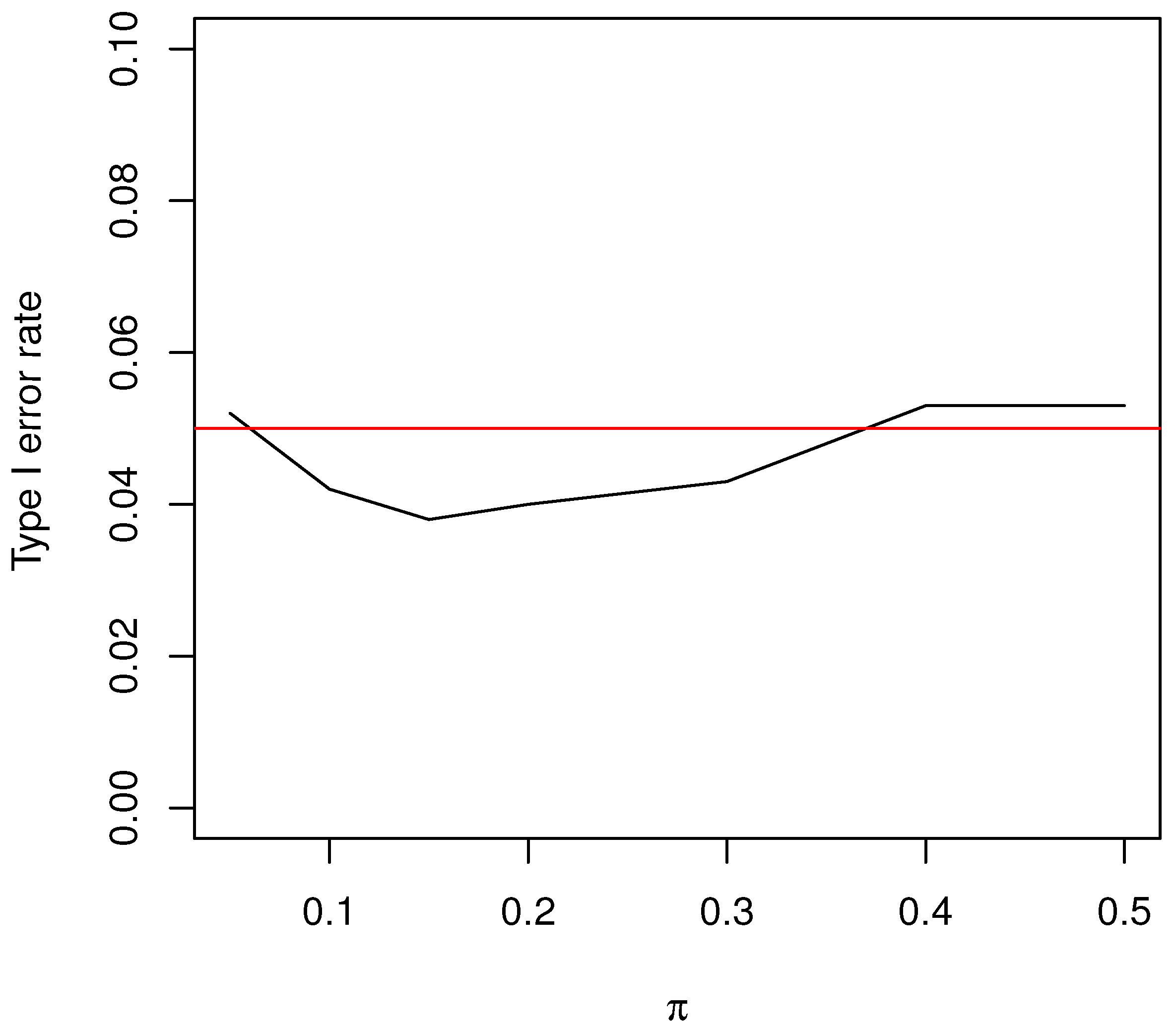
Figure 1. The type I error rates of the LRT for testing H 0 : θ = 0 against H 1 : θ > 0 .
Mathematics 13 02973 g001
Figure 2. The type I error rates of the LRT for testing H 0 : θ = 0 against H 1 : θ > 0 .
Mathematics 13 02973 g002
Figure 3. The power of the LRT for testing H 0 : θ = 0 against H 1 : θ > 0 .
Mathematics 13 02973 g003
Table 1. Point and confidence interval estimates with non-compliance parameter θ = 0.3 and n 1 = n 2 = 1000 .
Variant PICT with Non Compliance ( VPICT )
π ^ θ ^ λ ^ Width of CI
π = 0.05 0.08790.39041.99350.2823 (92.6%)
π = 0.10 0.12460.36041.99610.3087 (94.6%)
π = 0.20 0.20310.34472.00260.3495 (97.5%)
π = 0.30 0.30180.31682.00530.3757 (95.9%)
π = 0.40 0.40210.30972.00380.3848 (96.4%)
Note: Values in parentheses represent the exact coverage percentages.
Table 2. Point and confidence interval estimates with non-compliance parameter θ = 0.4 and n 1 = n 2 = 1000 .
Variant PICT with Non Compliance ( VPICT )
π ^ θ ^ λ ^ Width of CI
π = 0.05 0.07050.45591.99670.2084 (93.9%)
π = 0.10 0.10990.43811.99760.2323 (96.5%)
π = 0.20 0.20290.42362.00020.2671 (95.6%)
π = 0.30 0.30110.41191.99880.2796 (95.1%)
π = 0.40 0.40170.40712.00130.2814 (95.0%)
Note: Values in parentheses represent the exact coverage percentages.
Table 3. Observed answers and frequencies for Groups 1 and 2.
Group 1 Group 2
Observed Answers Frequency Observed Answers Frequency
07015
132137
252255
348343
424426
51957
61064
72
91
Table 4. Parameter estimates and confidence interval.
π ^ λ ^ θ ^ 95 % C.I. for π
Direct Questioning0.0057Not applicableNot applicable(0, 0.0169)
VPICT0.1932.0770.404(0, 0.7256)
Disclaimer/Publisher’s Note: The statements, opinions and data contained in all publications are solely those of the individual author(s) and contributor(s) and not of MDPI and/or the editor(s). MDPI and/or the editor(s) disclaim responsibility for any injury to people or property resulting from any ideas, methods, instructions or products referred to in the content.