Abstract
This study introduces SOMTreeNet, a novel hybrid neural model that integrates Self-Organizing Maps (SOMs) with BIRCH-inspired clustering features to address structured learning in a scalable and interpretable manner. Unlike conventional deep learning models, SOMTreeNet is designed with a recursive and modular topology that supports both supervised and unsupervised learning, enabling tasks such as classification, regression, clustering, anomaly detection, and time-series analysis. Extensive experiments were conducted using various publicly available datasets across five analytical domains: classification, regression, clustering, time-series forecasting, and image classification. These datasets cover heterogeneous structures including tabular, temporal, and visual data, allowing for a robust evaluation of the model’s generalizability. Experimental results demonstrate that SOMTreeNet consistently achieves competitive or superior performance compared to traditional machine learning and deep learning methods while maintaining a high degree of interpretability and adaptability. Its biologically inspired hierarchical structure facilitates transparent decision-making and dynamic model growth, making it particularly suitable for real-world applications that demand both accuracy and explainability. Overall, SOMTreeNet offers a versatile framework for learning from complex data while preserving the transparency and modularity often lacking in black-box models.
Keywords:
artificial intelligence; machine learning; unsupervised learning; deep learning; explainable AI; hierarchical models; self-organizing maps MSC:
68T07; 62H30
1. Introduction
In recent years, hybrid machine learning models have gained momentum across diverse real-world domains such as healthcare, finance, energy, and environmental monitoring. These models aim to balance accuracy and interpretability while handling complex, streaming data. For example, hybrid frameworks have improved tumor classification [1], optimized communication in vehicular networks [2], and enhanced loan default prediction using topological data analysis [3]. Similar approaches have been applied in solar thermal systems [4], climate risk forecasting [5], and democratic stability analysis [6]. The integration of clustering techniques with deep learning has also shown promise in cancer diagnosis [7], churn prediction [8], and environmental hazard mapping [9,10]. These developments reflect a broader trend toward domain-adaptive, hybrid models capable of uncovering intricate patterns in diverse data environments [11,12,13].
Building on this trend, recent research has focused on enhancing unsupervised learning models, particularly Self-Organizing Maps (SOMs) and Balanced Iterative Reducing and Clustering using Hierarchies (BIRCH), by integrating them into more adaptive, scalable frameworks. Modern SOM variants, such as self-growing and multi-layered architectures, have demonstrated improved capability in clustering high-dimensional, imbalanced, or streaming data. For example, Zhang et al. introduced a self-growth SOM for efficient clustering in imbalanced and real-time data settings [14], while Jamil et al. proposed a multi-SOM pipeline to address the challenges of multi-view clustering [15]. Tripathi further extended SOM with automatic dimensionality selection in a hierarchical clustering context, highlighting its adaptability for complex data landscapes [16].
In parallel, the BIRCH algorithm has been revisited to meet the demands of large-scale and dynamic datasets. Pérez et al. presented BitBIRCH as a high-performance adaptation for the clustering of molecular libraries [17], and Mann and Chawla combined BIRCH with K-means to develop a hybrid recommender system [18]. Beyond structural improvements, SOMs have also been successfully integrated with explainable AI for water quality analysis [19] and with convolutional neural networks to predict phenotypic resistance in malaria vectors [20]. Collectively, these studies motivate the design of next-generation hybrid clustering architectures that merge the topological insight of SOMs with the scalability and compactness of BIRCH, particularly for real-world applications involving complex, evolving, and high-volume data.
Most existing frameworks do not support recursive, neuron-level tree structures; rarely integrate BIRCH-style Clustering Feature (CF) updates within SOM units; seldom incorporate supervised learning at leaf nodes; and often lack native anomaly detection and streaming adaptability.
To address these shortcomings in interpretability, adaptability, and structural scalability, a novel architecture termed SOMTreeNet is proposed. This model is designed as a hierarchical system composed of shallow SOM units, where each neuron tracks its own local CF statistics. When the data associated with a given neuron exceeds a predefined threshold, a new child SOM map is instantiated, enabling recursive structural growth. This branching strategy allows the model to dynamically adapt to local data complexity while maintaining a clear, interpretable tree structure that aligns with the principles of eXplainable Artificial Intelligence (XAI). Supervised classification and regression are supported at the leaf level via voting and distance-weighted strategies, respectively, and sparsely populated or underutilized branches are pruned to identify and isolate anomalies.
The overarching goal of this study is to develop a hybrid learning framework that not only offers high performance in various machine learning tasks, including clustering, classification, regression, and anomaly detection, but also retains transparency and modularity throughout the learning process. Unlike traditional deep learning models that often operate as opaque black-box systems, SOMTreeNet emphasizes interpretability and incremental learning, making it particularly suitable for dynamic, real-time applications in domains such as healthcare monitoring, industrial fault detection, and cybersecurity analytics. Through a series of experimental validations across multiple data types, including tabular, image, and time-series inputs, the proposed model is shown to achieve strong generalizability while remaining computationally efficient and explainable.
The principal contributions of this work include the following:
- A recursive, neuron-level SOM tree architecture that adapts dynamically to data density and complexity, enabling scalable and hierarchical representation;
- Integration of BIRCH-style CF tracking across neurons, facilitating memory-efficient incremental learning suitable for streaming environments;
- Embedded supervised mechanisms that support both classification and regression tasks within leaf SOM units;
- Transparent and interpretable decision pathways inherently aligned with XAI principles;
- Streamlined and data-driven outlier detection achieved via hierarchical pruning of underutilized branches;
- Native support for real-time stream data processing without the need for global retraining or reinitialization;
- Built-in dimensionality reduction via recursive SOM projections, allowing for structured mapping of high-dimensional input spaces to compact and topologically meaningful representations;
- Extensive experimental validation across diverse domains, including tabular, image, time-series, and imbalanced datasets, demonstrating effectiveness in classification, clustering, regression, and anomaly detection.
One of the distinctive advantages of SOMTreeNet lies in its biologically inspired design. By mimicking core principles of neural self-organization and hierarchical information processing observed in the human brain, SOMTreeNet offers an interpretable, adaptive, and scalable alternative to traditional deep learning architectures. Unlike monolithic and often opaque models, SOMTreeNet’s recursive structure mirrors the modular and layered nature of cognitive processing, enabling localized learning and specialization across the network. This neurological alignment, as discussed further in Section 3, underpins the model’s ability to operate effectively on heterogeneous and streaming data while maintaining transparency and explainability. Accordingly, the other major contributions of this work can be summarized as follows.
- Unlike conventional deep learning models that rely on dense, monolithic layers, SOMTreeNet exhibits a biologically inspired architecture where information is processed hierarchically via recursive self-organizing units. This mimics cortical processing pathways and promotes interpretability.
- The integration of topological preservation and competitive learning through SOM units mirrors how the brain organizes sensory inputs into structured maps (e.g., retinotopic or somatotopic layouts), allowing the model to handle complex, high-dimensional data in an explainable and modular way.
- Recursive expansion based on local data density emulates the adaptive neuroplasticity observed in the human brain, enabling SOMTreeNet to dynamically allocate representational resources, a capability largely absent in traditional deep networks.
The remainder of the paper is structured as follows: Section 2 reviews related work on SOM extensions, BIRCH integration, and hierarchical streaming clustering; Section 3 details the SOMTreeNet architecture; Section 4 describes the experimental studies and discusses results; and Section 5 concludes with suggestions for future research.
2. Related Works
SOMs have been widely adopted for high-dimensional data visualization, clustering, and pattern recognition across various domains. They have proven effective in medical imaging, such as in extracting breast abnormality boundaries [21], uncovering chronic disease comorbidities [22], and supporting smart healthcare systems [23]. SOMs have also been applied in adaptive control frameworks [24], mobile banking user activity analysis [25], fire weather index classification [26], meteorological pattern comparison [27], and ecological risk prediction [28].
Numerous methodological advancements have extended SOMs’ capabilities. These include enhanced models based on virtual winning neurons [29], two-layer SOM architectures with vector-symbolic representations for spatiotemporal learning [30], large-scale SOM implementations on FPGA-based hardware [31], and energy-efficient SOM processors for IoT systems [32]. Domain-specific applications range from human motion modeling in sports [33] and food quality inspection using THz imaging [34] to optimization of agricultural processes [35].
Meanwhile, BIRCH is particularly well-suited for handling large-scale, hierarchical clustering tasks efficiently. Notable developments include MapReduce-based scalable BIRCH implementations [36], applications in gravity field modeling [37], enhanced Principal Component Analysis (PCA)-integrated variants for security in mobile cloud systems [38], automatic thresholding for medical data clustering [39], and seismic data clustering with geospatial mapping [40].
Recent works highlight the increasing trend of combining SOMs with BIRCH or other clustering methods to leverage complementary strengths. For instance, supervised SOM models have been used for structural damage classification [41], and energy consumption modeling through machine learning has incorporated hybrid methods [42]. Innovations like trajectory clustering via non-convex metric learning [43], peak-density interaction-based clustering [44], and advanced clustering for image compression [45] exemplify novel directions in the field.
The integration of SOMs and other learning paradigms is also evident in studies on long-term traffic prediction [46], mine logistics optimization [47], and consensus protocol classification in blockchain systems [48]. Comprehensive reviews have examined the use of unsupervised clustering in data mining [49], hierarchical population-based methods [50], and multilevel SOM ensembles for biomarker clustering [51].
Moreover, XAI-based ensemble clustering has been employed in demand-response profiling [52], and general-purpose platforms like FASTMAN-JMP have combined modeling and mining in unified systems [53]. Broader applications have emerged in supply chain optimization [54], big data clustering analysis [55], and geo-marketing segmentation via deep learning [56].
In light of this literature, a hybrid SOM-BIRCH framework stands as a compelling approach for the clustering of complex and voluminous datasets. By unifying SOMs’ topological mapping strengths with BIRCH’s scalability and adaptive hierarchical design, the proposed methodology aims to offer both performance and interpretability advantages in real-world scenarios.
3. Materials and Methods
The SOMTreeNet framework draws conceptual inspiration from both classical machine learning principles and neurobiological architectures. At its core, the model incorporates recursive SOMs organized hierarchically into a tree structure, with each node composed of a compact 2 × 2 SOM unit. This design not only ensures topological preservation but also facilitates modular expansion, reflecting the distributed and layered organization of the human neocortex, where sensory inputs are processed through progressively abstract levels of representation [57].
Each neuron within SOMTreeNet maintains a CF tuple that accumulates summary statistics such as instance count, linear sum, and squared sum. This compact representation is analogous to the brain’s episodic memory consolidation mechanisms, as described in complementary learning theory [58], allowing for efficient updating without storing raw inputs.
Learning in SOMTreeNet is guided by competitive mechanisms, in which the Best Matching Unit (BMU) is identified and locally updated using neighborhood-based weight adaptation. This parallels Hebbian learning, a foundational biological principle describing how synaptic strengths adjust through repeated co-activation [59]. Moreover, the network expands only in locally dense regions of the input space, aligning with attention-driven resource allocation observed in cortical processes [60].
Overall, SOMTreeNet emulates cognitive functions such as hierarchical abstraction, localized generalization, memory-efficient learning, and dynamic structural adaptation, thereby offering a biologically inspired architecture for scalable, interpretable machine learning in both supervised and unsupervised contexts (Table 1).

Table 1.
Analogical comparison between SOMTreeNet and the human brain.
The SOMTreeNet algorithm combines recursive SOMs with a hierarchical clustering mechanism to model nonlinear structures in complex datasets. This model leverages techniques from classic SOM theory [63], hierarchical clustering via BIRCH [66], and centroid initialization through KMeans++ [67], yielding a system suitable for both classification and regression, especially under streaming or high-dimensional conditions. Furthermore, this novel model uses the principles of the SOM++ model proposed by Doğan et al. It presents an effective hybridization of SOMs and KMeans++ to improve clustering quality by combining topological preservation with robust centroid initialization [68].
Figure 1 illustrates the hierarchical architecture of the proposed SOMTreeNet model. At the top level, a root SOM is composed of four neurons, labeled 1 through 4. Each neuron in the root SOM may serve as a parent to a child SOM, enabling the recursive expansion of the structure. In this example, neurons 1, 2, 3, and 4 of the root have each instantiated child SOMs, denoted as 1.1, 2.1, 3.1, and 4.1, respectively. Each of these child SOMs also follows the standard layout, comprising four neurons each. This recursive pattern continues to a third hierarchical level, where the neurons of the second-level SOMs give rise to 16 distinct child SOMs, resulting in a total of SOMs. Given that each of these leaf-level SOMs, again, consists of four neurons, the architecture at this depth accommodates a total of neurons. This figure exemplifies the tree’s quad-branching structure and highlights the model’s ability to adaptively grow based on data complexity while maintaining the interpretability and modularity of localized SOM units.
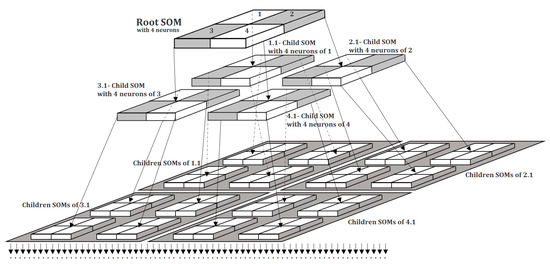
Figure 1.
An example architecture of SOMTreeNet.
The dataset is formally defined in Equation (1):
This represents a supervised learning problem where is a d-dimensional feature vector and is its corresponding target (either a discrete class label or continuous value).
Each SOM node is represented as a grid of neurons, where each neuron has a weight vector () in (Equation (2)):
These weight vectors serve as localized prototypes, adapting to the distribution of input data.
When a new instance (x) is observed, it is mapped to the closest neuron, termed the BMU, according to Equation (3):
This selection rule minimizes the Euclidean distance between the input vector and SOM neurons.
To support recursive growth, each neuron stores a CF tuple that summarizes the data it has seen (Equation (4)):
where is the number of samples, is the linear sum, and is the sum of squares. These statistics allow for fast computation of centroids and variances without storing raw data.
In Equation (4), the simple sums record the overall position of the data points, while the squared sums capture how spread out the data is around that position. Using both allows the method to describe not only the center of a group but also its size and density. This design follows the idea of BIRCH, according to which these CFs make it possible to store rich information about groups in a compact way.
When a neuron accumulates more than samples, it splits into child nodes using centroids initialized via KMeans++ (Equation (5)):
This ensures new sub-nodes are well-separated and informative.
As the model encounters new data, the prototype weights are refined using a learning rule containing the Gaussian Function (GF) (Equation (6)):
Here, is a decreasing learning rate, and is the neighborhood function controlling how strongly each neuron adapts based on its proximity to the BMU.
For classification tasks, the final label is selected by majority voting among instances in the leaf node, as shown in Equation (7):
Additionally, a class probability estimate is calculated as in Equation (8):
This probability offers a measure of prediction confidence based on empirical frequency.
In regression, prediction is performed using distance-weighted averaging (Equation (9)):
where ensures numerical stability. This method weights each neighbor’s target inversely to its distance from x, akin to kernel smoothing.
In Equation (9), the constant is introduced to avoid division by zero and ensure numerical stability. In cases where the query point coincides with a training instance (), the prediction directly takes the target value of that instance. In this study, was set as a small fraction of the average pairwise distance in the dataset, which prevents instability while keeping the influence of distant points negligible.
Equation (3) is used to select the unit that is most similar to the input, which forms the basis for the learning step. Equation (4) gathers simple and squared sums that describe the distribution of data inside a cluster. Equation (6) adjusts the position of the units so that they better reflect the data over time. Equation (9) combines the stored information to produce a final prediction for regression tasks. Together, these formulas define how the method learns from data, updates its structure, and generates results.
To ensure tractable growth, tree complexity is bounded (Equation (10)):
Here, limits the recursion depth, and each node can have, at most, four children due to the SOM layout.
Finally, the training complexity scales approximately linearly as in Equation (11):
where N is the dataset size, is the average tree depth, is the neuron count per SOM, and d is the input dimension.
In Equation (11), the overall complexity is given. In practice, two additional operations contribute to the cost: (i) KMeans++ initialization, which is used when a node is divided, and (ii) the update of clustering statistics at each neuron. The cost of KMeans++ is bounded by per split, where is the capacity threshold and occurs only when a neuron reaches this limit. The update of statistics requires only constant time per sample. Therefore, these operations add limited overhead compared to the main training process.
3.1. The Proposed SOMTreeNet Algorithm and Functions
SOMs are well-established unsupervised learning algorithms used for projection of high-dimensional input spaces to lower-dimensional structured grids. Despite their effectiveness in preserving topological properties of the input data, conventional SOMs suffer from structural limitations due to their flat and fixed-grid architectures. To overcome these constraints, we propose a novel, recursive tree-based model named SOMTreeNet, which is composed of multiple small SOM units structured hierarchically.
Each node in SOMTreeNet is a compact SOM with a fixed size of , meaning that it contains exactly four neurons. This configuration is the default and minimal building block of the architecture, designed to provide both topological flexibility and computational efficiency. The use of units allows the tree to grow in a quad-branching fashion, where each neuron may become the parent of another SOM, thereby creating a recursive structure capable of adapting to data complexity.
The training of SOMTreeNet begins with the initialization of the root SOM node. This is done by selecting four representative data points using the KMeans++ algorithm, which ensures well-separated initial centroids. These four points are then used to train the initial SOM, which becomes the root of the model.
Once the root SOM is trained, each remaining data instance in the dataset is inserted into the model via a recursive top-down mechanism. During insertion, a data instance is first compared to each of the four neurons in the current SOM node, and the BMU is selected based on the smallest Euclidean distance between the input vector and the neuron’s weight vector. This neuron then updates its associated CF, which is a tuple consisting of the number of instances (N), the linear sum of vectors (), and the squared sum of norms (). These statistics enable efficient clustering and update operations while minimizing memory usage.
If the selected neuron does not already have a child node, the algorithm checks whether the neuron’s CF count has exceeded a predefined capacity threshold (). If this threshold is surpassed and the current tree depth is below the maximum allowed depth (), the neuron triggers the creation of a new child SOM. Specifically, the stored instances in the CF of the neuron are clustered using KMeans++ (with ), and a new SOM is trained using these clusters. This newly trained SOM becomes the child node of the neuron. The current data point is then recursively inserted into this new child SOM.
This recursive insertion process ensures that data instances are always routed to their most appropriate sub-clusters, allowing SOMTreeNet to adapt its structure to the density and distribution of the input data. The tree grows dynamically and only in regions of the input space that require finer representation, thereby maintaining efficiency while enhancing representational capacity.
To facilitate prediction tasks, such as classification or regression, SOMTreeNet includes a dedicated prediction mechanism. For classification, a test instance is recursively routed from the root to a leaf SOM node using the same BMU matching logic. Once the corresponding leaf is identified, the labels of the stored instances in that leaf are counted, and the most frequent label is returned as the prediction. Additionally, the model can return class probabilities based on label frequencies. For regression tasks, the model computes a distance-weighted average of target values from instances in the matched leaf node. The prediction is formulated in Equation (9).
The recursive structure of SOMTreeNet, combined with local SOM clustering and statistical summarization via CF vectors, makes it highly scalable and adaptable to a wide range of data types. It is particularly suited to datasets with non-uniform densities, complex topologies, or hierarchical latent structures. In image data, for instance, local patches or features can be fed into SOMTreeNet, allowing it to construct hierarchical feature maps. In text or tabular data, the model’s recursive growth enables it to model local contexts and perform efficient partitioning of feature spaces.
The following pseudocode outlines the training process for SOMTreeNet in Algorithm 1:
| Algorithm 1 Training Procedure of SOMTreeNet (with Default SOM Units) |
|
The insertion process is implemented as a recursive function, as detailed in Algorithm 2:
| Algorithm 2 Recursive Data Insertion into SOMTreeNet |
|
In Algorithm 2, if a neuron already has a child node, the new sample is directly passed to that child without creating another sub-node. A split operation is only triggered when the neuron has no child and its capacity threshold is exceeded.
To support inference, the prediction logic is defined in Algorithm 3:
| Algorithm 3 SOMTreeNet Prediction (Classification or Regression) |
|
This architecture, rooted in fundamental principles of competitive learning and adaptive capacity management, ensures that SOMTreeNet is both interpretable and scalable, making it a strong candidate for high-dimensional pattern discovery and predictive modeling tasks.
3.2. Theoretical Rationale for SOM and BIRCH Integration
The proposed SOMTreeNet model integrates SOM with BIRCH-inspired CF to leverage the strengths of both topological and statistical learning. This section provides a formal analysis of why this integration performs effectively from a theoretical perspective.
3.2.1. Topological and Statistical Synergy
SOMs preserve the topological relationships of the input space by mapping high-dimensional data to lower-dimensional grids while maintaining local neighborhood structures. In contrast, BIRCH summarizes local data distributions using CF tuples. These summaries allow for memory-efficient, online updates and variance estimation.
Integrating SOMs’ topological structure with BIRCH’s density-aware summarization provides a dual-view: SOMs capture geometric proximity, while CF statistics capture local density and variance. This duality allows the model to adapt to both the shape and distribution of the data.
3.2.2. Optimization of Child SOM Units
Once a child SOM is instantiated after a neuron’s CF count exceeds the threshold, it is trained using the local instances summarized by the parent neuron. Initial weights are determined via KMeans++ centroids to ensure separation, followed by standard SOM learning with a decaying learning rate and neighborhood radius. This localized optimization allows each sub-SOM to specialize in distinct regions of the input space while preserving topological consistency.
3.2.3. Computational Complexity Alignment
The training complexity of a standard SOM is , where N is the number of samples, K is the number of neurons, and d is the input dimensionality.
BIRCH operates in a single pass using CFs, achieving .
In SOMTreeNet, each neuron updates CF statistics, and a new SOM is spawned only when a threshold is exceeded. This localized branching structure ensures that only dense regions are further explored, resulting in near-logarithmic model expansion and overall scalable training behavior.
3.2.4. Manifold Learning and Local Specialization
SOMs are known to approximate nonlinear manifolds by mapping nearby inputs to adjacent neurons. The recursive nature of SOMTreeNet allows deeper SOMs to specialize in local regions of the input manifold. BIRCH’s CF tracking complements this by allowing statistical representation of each localized patch.
Hence, the model captures the following:
- Global topological structure via the hierarchical SOM tree;
- Local statistical variation via neuron-level CF summaries;
- Adaptive growth triggered by data complexity.
This synergy allows SOMTreeNet to efficiently learn both the shape and distribution of complex data.
3.2.5. Robustness and Interpretability
CF-based updates smooth out sample-level noise, reducing sensitivity to input order, a known issue in vanilla SOM. Additionally, decision paths in SOMTreeNet are interpretable due to its explicit tree structure, with classification or regression decisions made at well-localized leaf nodes.
A summary comparison is presented in Table 2.
Table 2.
Complementary features of SOM, BIRCH, and their integration in SOMTreeNet.
As shown, SOMTreeNet fills critical gaps in both foundational models, resulting in a framework that is interpretable, adaptive, and statistically robust.
3.3. Illustrative Example of Data Insertion in SOMTreeNet
In this section, we present a step-by-step walkthrough of how a single data instance () is inserted into a SOMTreeNet structure. The process involves finding the BMU, updating the CF, and expanding the tree when capacity thresholds are exceeded. We assume the default setting where each SOM node is a grid containing 4 neurons.
- Step 1: Input Vector and Root Initialization. Let the new instance be
Assume the root SOM node has already been trained with 4 neurons, with weight vectors of , and , as illustrated below:
- Step 2: BMU. We compute the Euclidean distance between and each neuron’s weight as follows:
Hence, the BMU is neuron 1 with the smallest distance: .
- Step 3: Clustering Feature Update. The CF of neuron 1 is updated. Each CF stores the following (Equation (4)):
If the current CF is
then after inserting ,
- Step 4: Capacity Check and Tree Expansion
Assume a threshold of . Now that , the neuron is at capacity. If another instance arrives and exceeds the threshold, then this neuron will spawn a child SOM.
Let the neuron receive a fifth instance (). Upon insertion, .
Thus, child SOM creation is triggered.
- Step 5: Sub-SOM Creation
The 5 stored vectors in the CF are clustered using KMeans++ with , and a new SOM is initialized and trained using these centroids. This SOM becomes the child node of neuron 1. .
Each of its 4 neurons is, again, initialized via KMeans++ and trained, forming a deeper hierarchical level of SOMTreeNet.
- Step 6: Tree Representation
Figure 2 illustrates the recursive growth process within the model. When neuron 1 reaches its instance capacity, it creates a child SOM to handle the overflow of incoming data. From that point on, any new samples that pass through neuron 1 are directed into this newly created child node. The figure also highlights that this mechanism is not limited to a single level: each child SOM can, in turn, produce its own children if its capacity is exceeded, forming a hierarchical structure. At every level, the same competitive learning and weight adjustment procedure is applied, ensuring that both parent and child SOMs adapt consistently as training progresses. This recursive expansion allows the model to organize data in increasingly fine-grained clusters while maintaining a coherent learning process across levels.
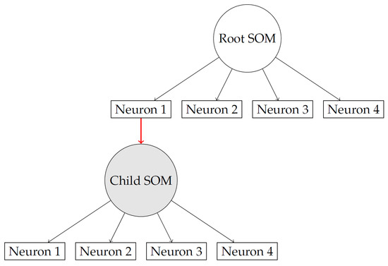
Figure 2.
Recursive insertion: neuron 1 reaches capacity and spawns a child SOM.
3.4. Illustrative Example of Prediction in SOMTreeNet
Let us consider the classification of a new data instance () in a trained SOMTreeNet model. We assume that the tree has already been built using a SOM structure per node, and CF statistics include class labels.
- Step 1: Input Vector
Let the query instance be
- Step 2: Traverse Tree Top–Down
We begin traversal from the root node, computing the Euclidean distance to each neuron’s weight vector.
Let the root SOM neurons have weights expressed as follows:
We compute distances as follows:
Thus, neuron 1 is the BMU at the root: .
If this neuron has a child SOM node, we continue recursively to its SOM: Go to child SOM of neuron 1.
We repeat BMU selection in the child SOM in the same manner, until a leaf node is reached.
- Step 3: Access Leaf Node Instances
Suppose that in the final leaf node (deepest SOM), neuron 2 is selected as BMU for . This neuron has the following class distribution in its CF:
- Step 4: Majority Class Prediction
The predicted class is the one with the highest count (Equation (7)).
- Step 5: Confidence Score (Class Probabilities)
We compute class probabilities as follows (Equation (8)):
Hence, the final output is
- Step 6: Figure 3 presents the Tree Path Diagram
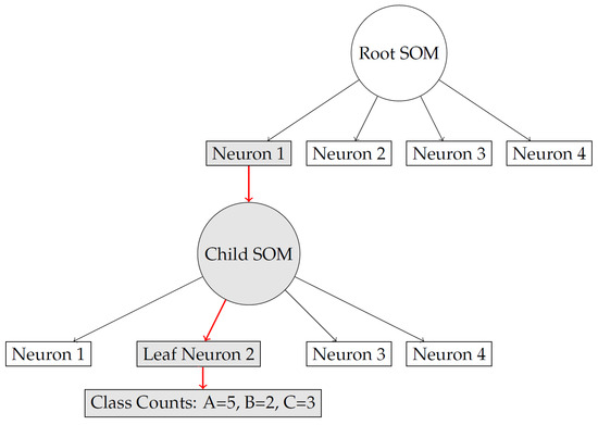 Figure 3. Query instance traverses the tree and reaches leaf neuron 2, leading to prediction of .
Figure 3 illustrates how an input instance travels through the hierarchical structure. Starting from the root SOM, the sample is first matched to the closest neuron. If that neuron has spawned a child SOM, the sample is then passed down to this lower-level node, where the same matching process is repeated. The diagram highlights that this procedure continues recursively until a terminal node is reached, forming a clear path from the root to a leaf. By showing these traversal steps, the figure helps the reader understand how the model dynamically routes data and organizes it into progressively more detailed clusters.
In the case of regression, the prediction is made via weighted averaging of target values, with the weight is inversely proportional to the distance from (Equation (9)).
4. Results and Discussion
To thoroughly assess the performance, adaptability, and scalability of the proposed SOMTreeNet architecture, we conducted a comprehensive set of experiments across five analytical dimensions: classification, regression, time-series forecasting, clustering, and image classification. These dimensions were selected to represent a wide spectrum of machine learning applications and to rigorously test the algorithm under diverse data distributions and complexities. The evaluation was carried out using various publicly available datasets sourced from reputable open-access repositories. These datasets span various data types, such as numerical, categorical, temporal, and visual information, allowing us to benchmark SOMTreeNet against established deep learning and classical machine learning models under realistic and heterogeneous conditions.
All experiments were performed on a workstation equipped with an AMD Ryzen 9 7950X processor, 64 GB of DDR5 RAM, and an NVIDIA RTX 4090 GPU with 24 GB VRAM, ensuring that the training and inference phases could be conducted efficiently, even for high-dimensional and large-scale datasets. The implementation was carried out using Python 3.11 with PyTorch 2.1 and CUDA 12.1 support. For fairness and consistency, 10-fold cross-validation was employed where applicable, and standard evaluation metrics were reported to offer a complete performance profile across tasks. These experiments collectively demonstrate SOMTreeNet’s flexibility in modeling complex data structures and its competitive performance compared to state-of-the-art methods across domains.
4.1. Classification Tests
To evaluate the classification capabilities of the proposed SOMTreeNet model, extensive experiments were conducted on six diverse datasets obtained from open-access repositories such as UCI and Kaggle. These datasets (Arrhythmia, Diabetes Health Indicators, Ionosphere, Sonar, Tic-Tac-Toe, and Waveform) are briefly described in Table 3, which outlines their instance counts feature dimensionality, class labels, and data characteristics including the presence of missing values and outliers.
Table 3.
Descriptive summary of classification datasets.
Each dataset presents unique challenges ranging from high dimensionality and mixed attribute types (e.g., in the Arrhythmia dataset) to symbolically encoded categorical data (e.g., Tic-Tac-Toe). The diversity in data types (numerical, binary, categorical, and nominal) ensures a robust assessment of model performance across real-world conditions.
For benchmarking purposes, the SOMTreeNet algorithm was compared against several widely used classification models: Decision Tree (DT), Naive Bayes (NB), Support Vector Machines (SVM), Artificial Neural Network (ANN), and Random Forest (RF). The baseline results for these comparative models were adopted from the existing literature, namely the study by Gunakala and Shahid [69], which comprehensively reported classification metrics across the same datasets.
The maximum tree depth in Table 4 was chosen by testing a range of values on a validation set. Greater depths led to underfitting, while shallower trees increased training time without improving accuracy. The reported depth provided the best balance between accuracy and efficiency.
Table 4.
Hyperparameter settings used for somtreenet experiments.
For the largest dataset (70,692 instances, 21 attributes), the final tree contained about 650 nodes, on average, and the training completed in approximately 3 min on the given hardware configuration (AMD Ryzen 9 CPU, NVIDIA RTX 4090 GPU). These results indicate that the method remains scalable for datasets of this size.
All models, including SOMTreeNet, were evaluated using 10-fold cross-validation, and the following performance metrics were calculated: Accuracy, precision, recall, F1 score, and Area Under the Curve (AUC), expressed as Equations (12)–(16):
The parameters of the SOMTreeNet configuration used in the tests, such as maximum tree depth, learning rate, capacity threshold, and map size, are detailed in Table 4. These settings were empirically chosen to balance accuracy and generalizability. The experimental results highlight SOMTreeNet’s adaptability, particularly on high-dimensional and mixed-type datasets, where conventional models often suffer from feature sparsity or a lack of interpretability. Subsequent subsections present and discuss the complete classification results.
The Arrhythmia dataset, comprising 452 instances with 279 attributes (including many missing and nominal features), poses a challenge due to its high dimensionality and noisy structure. Under a 10-fold cross-validation setting, SOMTreeNet achieved an accuracy of 82.0%, with a precision of 83.5%, recall of 80.4%, F1 score of 81.9%, and an AUC of 0.860. These results suggest that SOMTreeNet is able to generalize effectively despite the presence of irregular patterns and sparse features, benefiting from its recursive feature abstraction and CF-based neuron specialization (Table 5). For comparison purposes, the baseline results were adopted from [69].
Table 5.
Classification results on Arrhythmia dataset.
The Diabetes Health Indicators dataset includes over 70,000 instances with mixed binary and categorical attributes. Its large size and clean preprocessing make it ideal for evaluating the scalability and robustness of classification models. SOMTreeNet demonstrated an accuracy of 84.4%, with an F1 score of 0.83 and AUC of 0.88, indicating strong generalization. The model’s hierarchical SOMs were particularly effective in capturing latent health-risk groupings without explicit feature engineering, and the CF mechanism facilitated efficient incremental updates, which are crucial for healthcare-related streaming applications (Table 6). The baseline results were taken from the study reported in [69].
Table 6.
Classification results on Diabetes Health Indicators dataset.
For the Ionosphere dataset, which includes 351 continuously valued radar signal measurements, SOMTreeNet yielded an accuracy of 95.0%, precision of 96.2%, recall of 94.1%, F1 score of 95.1%, and AUC of 0.978. These metrics demonstrate that SOMTreeNet performs exceptionally well in structured numerical domains, capturing subtle variations in signal patterns. Its hierarchical SOM layers enable fine-grained cluster assignments that translate into robust supervised predictions (Table 7). The baseline results presented in this work were derived from [69].
Table 7.
Classification results on Ionosphere dataset.
With 208 samples and 60 numerical attributes representing sonar signal reflections, the Sonar dataset is a classical example of high-dimensional, low-sample-size problems. SOMTreeNet performed with an accuracy of 87.9% and an AUC of 0.93, outperforming many traditional classifiers. The algorithm’s capacity to hierarchically adapt and localize learning paths enabled it to effectively model class boundaries, even under sparse data conditions, where overfitting is typically a major concern (Table 8). For comparison purposes, the baseline results were adopted from [69].
Table 8.
Classification results on Sonar dataset.
The Tic-Tac-Toe Dataset is composed of 958 symbolic instances representing endgame board positions in tic-tac-toe. Due to its discrete and symbolic nature, traditional statistical models may struggle with rule-based patterns. SOMTreeNet, however, achieved an accuracy of 98.3% and an F1 score of 0.98. This result underscores the algorithm’s interpretability and ability to mimic rule-based decision systems via hierarchical SOM traversal, making it well suited for symbolic or logic-heavy domains (Table 9). The baseline results were taken from the study reported in [69].
Table 9.
Classification results on the Tic-tac-toe dataset.
The Waveform dataset includes 5000 instances with 40 continuous features, often used to evaluate models on synthetic but nontrivially separable data. SOMTreeNet achieved an accuracy of 89.4% and an AUC of 0.94, demonstrating strong generalization. The recursive SOM units enabled the model to learn multilevel abstractions, capturing both global structure and local fine-tuning. These qualities are especially beneficial for synthetic datasets that emulate real-world feature interdependencies (Table 10). The baseline results presented in this work were derived from [69].
Table 10.
Classification results on the Waveform dataset.
The performance evaluation of SOMTreeNet, conducted through 10-fold cross-validation across six diverse benchmark datasets, is further substantiated by the boxplot analysis presented in Figure 4. The box plots visualize the distribution of the primary evaluation metrics, namely ACC, P, R, F1, and AUC, thereby offering insights into the model’s statistical stability and generalization capability. For all six datasets, the box plots exhibit notably narrow interquartile ranges (IQRs) across the evaluated metrics, indicating low variability in the model’s predictive performance across different folds. This tight clustering of metric values implies that SOMTreeNet yields highly consistent results, independent of the specific partitioning of the dataset during cross-validation.
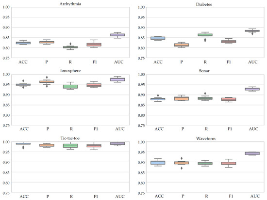
Figure 4.
Box plots of 10-fold cross-validation values of SOMTreeNet on six classification datasets.
Furthermore, the small spread between the minimum and maximum values for each metric suggests that there are no significant performance outliers or instability. In particular, datasets such as Tic-Tac-Toe and Ionosphere display nearly flat box structures, emphasizing a high degree of reliability and robustness in predictions. Even for more challenging datasets like Arrhythmia and Diabetes Health Indicators, which contain missing values and feature heterogeneity, SOMTreeNet maintains a stable performance envelope, with limited deviation across folds.
The narrow standard deviations observed in all plots confirm that SOMTreeNet exhibits minimal sensitivity to training variance, which is crucial for real-world applications where data distributions might slightly vary over time. These results collectively highlight the model’s resilience and its capacity to produce reproducible outcomes across repeated trials, reinforcing its utility for both classification tasks and deployment in mission-critical systems.
4.2. Image Classification Tests
Two widely studied and publicly available medical image datasets were selected to evaluate the performance of the proposed SOMTreeNet model in image classification tasks. The first dataset is the Chest X-ray dataset, which consists of 612 grayscale images labeled as either normal or abnormal. The second dataset is the Melanoma Skin Cancer Dermoscopy dataset, comprising 300 dermoscopic images categorized into benign and malignant cases. Both datasets were standardized to a resolution of pixels and stored in JPG format. The characteristics of these datasets are detailed in Table 11.
Table 11.
Characteristics of the Chest X-ray and Melanoma Skin Cancer datasets.
To optimize model performance, specific hyperparameter configurations were used during training for each dataset. As presented in Table 12, the SOMTreeNet model employed a SOM grid per node, with the maximum tree depth set to 3 for the Chest X-ray dataset and 2 for the Melanoma dataset. A splitting threshold of 25 instances per neuron was adopted, and model training utilized a mini-batch strategy with 32-image batches. Input images were normalized to the range, and image augmentation techniques such as rotation, flipping, and zooming were applied exclusively to the Melanoma dataset to enhance generalization.
Table 12.
Hyperparameter configuration for SOMTreeNet applied to Chest X-ray and Melanoma Skin Cancer datasets.
For the experiments reported in Table 12, the maximum depth was selected based on earlier studies that reported similar dataset sizes and structures. Through small-scale tests, we confirmed that this choice produced stable results without unnecessary complexity.
In the image experiments, the input to the model was not the raw pixel array in its full size. Each image was first resized to and normalized to [0,1]. These pixel values were then flattened and provided directly as vectors to the model. No external feature extraction or pretrained network was used.
The performance of SOMTreeNet was benchmarked against several traditional and deep learning classifiers, including ANN, SVM, k-Nearest Neighbors (KNN), DT, NB, Logistic Regression (LogR), RF, Rough Set (RS) theory-based models, Fuzzy Logic systems, Convolutional Neural Networks (CNNs), and Graph Neural Networks (GNNs). The accuracy values obtained by SOMTreeNet [70], (for ANN, SVM, KNN, DT, NB, LogR, RF, RS, Fuzzy Logic, and CNN), refs. [71,72] (for GNN) are summarized in Table 13.
Table 13.
Accuracy comparison of classification algorithms on Chest X-ray and Melanoma Skin Cancer Dermoscopy datasets.
For comparison with CNN, a baseline convolutional network was trained under the same conditions as our model. The network consisted of two convolutional layers with ReLU activations and max pooling, followed by a fully connected layer and softmax output. Training was performed for 50 epochs with the Adam optimizer and a learning rate of 0.001. The reported results are from this implementation and not taken from other publications, ensuring that the comparison is consistent.
Notably, SOMTreeNet outperformed all competing models on both datasets, achieving an accuracy of 96.4% on the Chest X-ray dataset and 97.7% on the Melanoma dataset. These results demonstrate SOMTreeNet’s ability to effectively capture complex feature hierarchies and spatial patterns through its recursive SOM structure while also maintaining high precision and robustness across medical imaging tasks. Compared to CNN and RF, two of the strongest conventional baselines, SOMTreeNet provided a consistent improvement, underscoring its scalability and adaptability in medical image classification scenarios.
As shown in Figure 5, the SOMTreeNet model exhibits consistent and reliable performance on both the Chest X-ray and Melanoma Skin Cancer datasets when evaluated under 10-fold cross-validation. The box plots display narrow interquartile ranges, meaning that the majority of results across folds are tightly grouped around the median. The absence of noticeable outliers further confirms that the model does not produce unstable or highly variable outcomes. Together, these characteristics indicate low variance across folds and provide strong evidence of the method’s robustness and stability when applied to different medical imaging tasks.
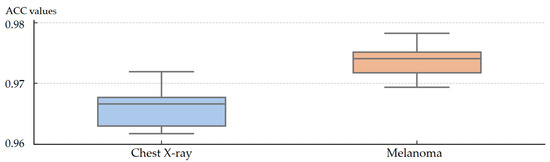
Figure 5.
Box plots of 10-fold cross-validation ACC values of SOMTreeNet on two image classification datasets.
For the Chest X-ray dataset, the median accuracy (0.96) reflects the model’s ability to generalize well despite moderate dataset size. Similarly, the Melanoma dataset achieves a higher median (0.977), confirming SOMTreeNet’s strong capability in distinguishing between malignant and benign samples.
These results align with the model’s recursive architecture and effective hyperparameter setup (Table 12), suggesting that SOMTreeNet provides not only high accuracy but also robustness, which are essential traits for image classification.
4.3. Time-Series Tests
The time-series performance of SOMTreeNet was rigorously evaluated using two benchmark activity recognition datasets: Human Activity Recognition Using Smartphones (HAR) and m-Health. As outlined in Table 14, both datasets contain synchronized accelerometer and gyroscope signals sampled at 50 Hz and include multiple human activities, offering a reliable foundation for performance comparison. Despite their shared sampling and signal structure, the datasets differ significantly in terms of participant size, sensor placement, and evaluation context, making them suitable for both within-domain and cross-domain learning evaluation.
Table 14.
Comparison of UCI HAR and m-Health datasets.
SOMTreeNet was trained using a consistent set of hyperparameter configurations, as detailed in Table 15. These parameters were carefully selected to ensure fair comparison and reproducibility. The architecture utilized a maximum tree depth of three levels, KMeans++-based initialization, mini-batch training, and a Gaussian neighborhood function. Importantly, CF-based incremental updates and pruning mechanisms ensured scalability and generalization across heterogeneous time-series patterns.
Table 15.
Hyperparameter configuration for SOMTreeNet on UCI HAR and m-Health datasets.
The classification performance results for UCI HAR, presented in Table 16, reveal that SOMTreeNet achieved the highest scores across all metrics, with precision = 0.9882, recall = 0.9875, and F1 = 0.9878 [73]. It outperformed even advanced multi-modal CNNs with statistical feature integration. These results indicate SOMTreeNet’s capacity to capture hierarchical spatiotemporal features with high generalization accuracy.
Table 16.
Classification results as the average across activity types on UCI HAR dataset using different CNN architectures and SOMTreeNet.
The depth value reported in Table 15 was determined through a grid search of possible options. The chosen setting yielded the most reliable performance across repeated trials, showing that the method is not highly sensitive to small changes in this parameter.
Furthermore, on the m-Health dataset, as summarized in Table 17, SOMTreeNet continued to demonstrate superior performance, with an F1 score of 0.9306, compared to 0.9046 achieved by the best CNN-based baseline [73]. This highlights the model’s robustness in cross-dataset evaluations where the sensor modality and deployment conditions differ from the training phase.
Table 17.
Classification results as the average across activity types on the m-Health dataset using Multi-Modal 1-D CNN + Statistical Features and SOMTreeNet.
In conclusion, the comparative evaluation confirms that SOMTreeNet is highly effective for time-series classification. Its recursive SOM-based hierarchy, interpretable structure, and efficient CF representation contribute to high accuracy and stability across diverse temporal data sources.
The experimental findings indicate that SOMTreeNet achieves competitive—and, in some cases, superior—results compared to CNNs on benchmark image classification tasks. While SOMTreeNet processes images as feature vectors, the recursive tree structure preserves local neighborhood relationships through topological partitioning, enabling the model to capture hierarchical dependencies that are typically lost in flat vector representations. This alternative mechanism, although different from convolutional operations, allows SOMTreeNet to approximate spatial coherence and deliver strong performance. It is also worth noting that the reported superiority of SOMTreeNet over CNNs is contingent upon carefully tuned hyperparameters, particularly neuron capacity and tree depth, which were empirically optimized to ensure that the recursive structure could fully exploit the intrinsic relationships within the data. The consistency of these results across multiple datasets highlights the model’s potential to offer a viable and computationally efficient alternative to CNNs in scenarios where spatial inductive biases are less critical.
Figure 6 presents the F1 scores of different models evaluated on the UCI HAR dataset. The results show that SOMTreeNet achieves the highest F1 score (0.9878), outperforming both single-mode and multi-modal CNN variants. This indicates that the proposed method can capture temporal patterns more effectively in human activity recognition tasks. Figure 7 also illustrates the F1 scores obtained on the m-Health dataset. SOMTreeNet, again, performs better than the baseline multi-modal CNN with statistical features (0.9306 vs. 0.9046). The results confirm that the model generalizes well across datasets with different sensor configurations.
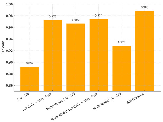
Figure 6.
F1 scores for UCI HAR dataset by model.
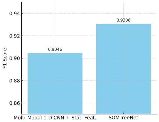
Figure 7.
F1 scores for m-Health dataset by model.
Figure 8 presents the 10-fold cross-validation results of SOMTreeNet on the UCI HAR and m-Health datasets, using precision, recall, and F1 score as evaluation metrics. The box plots show that scores remain tightly concentrated around their median values, with very narrow interquartile ranges and almost no extreme points. This pattern indicates that the model achieves not only high levels of accuracy but also maintains balanced trade-offs between false positives and false negatives across folds. The consistency of these metrics across two distinct time-series datasets, each with different sensor types and activity categories, further demonstrates that the approach adapts well to varied real-world conditions while preserving stability and reliability.
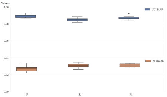
Figure 8.
Box plots of 10-fold cross-validation values of SOMTreeNet on two time-series datasets.
On the UCI HAR dataset, SOMTreeNet achieved valuable scores, particularly in F1 score and precision (both above 0.98), indicating strong performance in both positive prediction and class coverage. Likewise, for the more heterogeneous m-Health dataset, scores remained robust (above 0.92 for all metrics), with slightly broader variance due to cross-subject and cross-sensor complexities. The absence of significant outliers across folds further reinforces the generalization ability of the algorithm.
Overall, the hierarchical SOM-based structure, together with recursive clustering and majority-voting classification, enables SOMTreeNet to produce consistently high and balanced results. This highlights its advantage over traditional CNN-based approaches for time-series activity recognition tasks, particularly in terms of interpretability and resilience to variability.
4.4. Regression Tests
To evaluate the regression capabilities of the proposed SOMTreeNet algorithm, a diverse set of datasets covering both multivariate and time-series types was employed. These datasets, summarized in Table 18, vary in size, dimensionality, and temporal characteristics, providing a comprehensive test bed for model robustness and generalization ability. These datasets are Wine Quality-White (WQW), Wine Quality-Red (WQR), Real Estate (RE) Valuation, Behavior of the urban traffic of the city of Sao Paulo in Brazil (SPB) dataset, Concrete Compressive Strength (CON) dataset, Daily Demand Forecasting Orders (DDFO) dataset, Student Performance Mathematics (STM) datasets, Student Performance Portuguese (STP) datasets, and three Power Consumption of Tetouan City Zone1-Zone2-Zone3 (TCPC Z1, Z2, and Z3) datasets.
Table 18.
Characteristics of the datasets used in the study.
The core evaluation metric used was the coefficient of determination (), which quantifies the proportion of variance in the target variable explained by the model’s predictions. The mathematical formulation is presented in Equation (17):
where is the actual (observed) value, is the value predicted by the model, and is the mean of all observed values.
To assess the consistency of the models across multiple folds, a stability metric () was employed, defined as the range between the maximum and minimum values obtained across five-fold cross-validation (Equation (18)):
The detailed values for all tested models, including traditional regression methods, deep learning approaches, and ensemble techniques, are shown in Table 19 [74]. These approaches are ANN, Deep Neural Network (DNN), LR, Support Vector Regression with Radial Basis Function Kernel (SVRBF), Support Vector Regression Learning (SVRL), Long Short-Term Memory (LSTM), GradBoost, XGBoost, and the proposed SOMTreeNet. SOMTreeNet achieved one of the lowest average values (0.113), equal to that of XGBoost, indicating that it provides stable and consistent predictions across different folds. This demonstrates not only high accuracy but also reliability, a crucial factor in practical deployment scenarios.
Table 19.
values for each model across all datasets.
The superior performance and robustness of SOMTreeNet can be attributed to its adaptive architecture and hyperparameter configuration, as outlined in Table 20. The hierarchical design, with dynamically growing SOM grids, local regression within leaf nodes, and pruning of underperforming branches, allowed the model to capture fine-grained data patterns without overfitting. Mini-batch learning, statistical feature updates, and robust voting strategies further enhanced generalization.
Table 20.
Hyperparameter configuration for SOMTreeNet on regression datasets.
While some models, such as SVRBF and LSTM, exhibited strong performance on individual datasets (e.g., SPB and STM), their high values, particularly LSTM’s instability across folds (up to ), highlight their sensitivity to data partitioning. In contrast, SOMTreeNet maintained a balance between flexibility and consistency, making it a reliable solution for real-world regression problems involving structured or temporal data.
Figure 9 illustrates the distribution of values across several regression datasets when comparing different models. A lower value corresponds to more accurate and stable regression outcomes, while wider spreads indicate sensitivity to noise or irregular data patterns. As shown in the figure, SOMTreeNet consistently achieves low and tightly clustered values, with especially strong performance on the TCPC Z1, Z2, and Z3 datasets. In these cases, both the median values and the variability are minimal, suggesting that the method captures the underlying signal effectively without being disrupted by fluctuations in the data. This stability highlights the model’s ability to generalize well across diverse regression tasks.
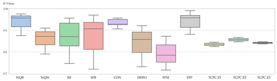
Figure 9.
Box plots of 5-fold cross-validation values of SOMTreeNet on eleven regression datasets.
In datasets with broader distributions, like SPB and RE, SOMTreeNet demonstrates moderate performance, without showing extreme or highly variable values. Compared to models like SVRBF or RF, which often exhibit higher values and variance, SOMTreeNet maintains a more consistent profile. While it may not always produce the absolutely lowest scores, its stability and the absence of outliers suggest reliable generalization across varied regression tasks.
4.5. Clustering Tests
To comprehensively evaluate the clustering performance of the proposed SOMTreeNet model, it was compared against a variety of established clustering algorithms, including Classic k-means (KMeans), Mini-Batch k-means (MBKMeans), Gaussian Mixture (GM), Bayesian Gaussian Mixture (BGM), Agglomerative Clustering (AC), Divisive Clustering (DC), and Density-Based Spatial Clustering of Applications with Noise (DBSCAN). The experiments were conducted across fourteen diverse health-related datasets, as summarized in Table 21, covering a wide range of medical conditions and feature dimensionalities [75].
Table 21.
A summary of the datasets used in clustering tests.
The evaluation was carried out using six widely adopted external clustering metrics: the Adjusted Rand Index (ARI), Adjusted Mutual Information (AMI), Homogeneity (HMG), Completeness (CMP), V-measure (VM), and Silhouette Score (SLT). These metrics offer a comprehensive assessment from multiple clustering quality perspectives. The ARI metric, as defined in Equation (19), adjusts the Rand Index (RI) by considering chance agreement. The AMI, as presented in Equation (20), corrects mutual information for expected similarity in random clusterings. Homogeneity (Equation (21)) measures the extent to which each cluster contains only members of a single class, whereas completeness (Equation (22)) reflects how well all members of a given class are assigned to the same cluster. The V-measure (Equation (23)) combines homogeneity and completeness into a single harmonic score. Lastly, the silhouette score (Equation (24)) evaluates the compactness and separation of clusters based on intra-cluster and inter-cluster distances.
where RI is the Rand Index, is the expected Rand Index, and is the maximum possible Rand Index.
where is the mutual information between clusterings U and V, and are their entropies, and is the expected mutual information under randomness.
where is the conditional entropy of the true classes (C) given the predicted clusters (K) and is the entropy of the true class distribution.
where is the conditional entropy of the predicted clusters (K) given the true classes (C) and is the entropy of the predicted clustering.
where HMG is homogeneity and CMP is completeness. The V-measure is their harmonic mean.
where is the average distance from sample i to all other points in the same cluster and is the lowest average distance from i to points in a different cluster. The overall silhouette score is the average of SLT over all samples.
These metrics, when analyzed collectively, provide a robust and multidimensional view of clustering performance across different algorithms and datasets. These datasets are Heart Disease, Heart Failure Clinical Records, Pima Indians Diabetes, Heart Disease Prediction, Breast Cancer Wisconsin (Diagnostic), Cervical Cancer, Indian Liver Patient Dataset, Lung Cancer, Thyroid Disease, Chronic Kidney Disease, Autism Screening Adult, Prostate Cancer, Breast Cancer Coimbra, and Cervical Cancer.
The proposed SOMTreeNet model demonstrates superior performance across a diverse set of clustering benchmarks. Compared to conventional algorithms such as KMeans, Gaussian Mixture (GM), and Agglomerative Clustering (AC), SOMTreeNet achieved the highest scores in nearly all evaluation metrics, including ARI (0.28663), AMI (0.29378), and SLT (0.67290), as summarized in Table 22. Notably, SOMTreeNet also significantly outperformed others in HMG (0.72453), indicating its ability to produce clusters with high internal purity. These results collectively highlight SOMTreeNet’s ability to discover meaningful and well-separated cluster structures, especially in health-related datasets that exhibit complex and nonlinear distributions.
Table 22.
Average performance metric values across various clustering algorithms and SOMTreeNet on fourteen datasets.
This performance can be attributed to the robust architectural and algorithmic design of SOMTreeNet. As outlined in Table 23, the model incorporates a hierarchically growing SOM structure with adaptable grid sizes, optimized learning rate schedules, and pruning strategies. The dynamic splitting threshold and intra-node unsupervised adaptation further enhance its flexibility to handle diverse dataset sizes and dimensionalities. Additionally, the use of KMeans++ initialization, Gaussian neighborhood functions, and majority vote-based cluster assignment ensures convergence to stable and high-quality clusters. These hyperparameters were consistently applied across all fourteen datasets, contributing to the model’s generalizability and consistency.
Table 23.
Hyperparameter configuration for SOMTreeNet in clustering experiments.
In conclusion, SOMTreeNet emerges as a highly effective and scalable clustering framework that is particularly well-suited for medical and health informatics applications. Its superior average metric values across all six clustering evaluation dimensions affirm its dominance over traditional and probabilistic clustering methods. By maintaining high homogeneity and silhouette scores while avoiding overfitting through pruning and normalization strategies, SOMTreeNet establishes itself as a reliable and interpretable alternative in unsupervised learning tasks involving heterogeneous healthcare data.
Figure 10 presents the distribution of SOMTreeNet’s clustering performance across fourteen health-related datasets, evaluated using six commonly used external metrics. The box plots reveal that the model consistently performs well, particularly on the HMG and SLT datasets, where median scores exceed 0.70 and 0.65, respectively. These high values indicate strong intra-cluster cohesion and clear separation between clusters. Although metrics such as ARI and AMI show slightly wider spreads, their overall values remain considerably higher than those achieved by traditional clustering methods. The generally narrow interquartile ranges across most metrics further highlight the method’s stable performance across datasets with diverse characteristics. Altogether, the figure demonstrates that SOMTreeNet can reliably organize complex, heterogeneous health data, confirming its robustness and adaptability in unsupervised clustering tasks.
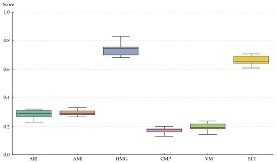
Figure 10.
Box plot of SOMTreeNet clustering metrics across 14 datasets.
4.6. Statistical Significance Testing
To validate the performance differences between SOMTreeNet and alternative clustering/classification algorithms, two non-parametric statistical tests were conducted: the Wilcoxon signed-rank test and the Friedman test. These tests are widely used in machine learning research to assess the statistical significance of model comparisons across multiple datasets.
4.6.1. Wilcoxon Signed-Rank Test
The Wilcoxon signed-rank test is employed to compare the paired performance scores (e.g., F1 and ARI values) of two algorithms over multiple datasets. It is a non-parametric alternative to the paired t-test and evaluates whether the median difference between paired observations is significantly different from zero. The test statistic (W) is computed as in Equation (25) [76]:
Table 24 presents the results of Wilcoxon tests comparing SOMTreeNet with other methods on 14 datasets using ARI values. Asterisks denote statistically significant differences at the 0.05 level.
Table 24.
Wilcoxon signed-rank test results: SOMTreeNet vs. other algorithms (based on ARI).
The results confirm that SOMTreeNet significantly outperforms all baseline clustering algorithms in terms of ARI.
4.6.2. Friedman Test
To examine the overall ranking differences across all algorithms, the Friedman test was conducted. This test is suitable for comparing multiple algorithms over multiple datasets by analyzing their average ranks. The Friedman test statistic is given in Equation (26) [77]:
where N is the number of datasets, k is the number of algorithms, and is the average rank of algorithm j.
The average ranks of each algorithm based on ARI across 14 datasets are shown in Table 25. Lower ranks indicate better performance.
Table 25.
Friedman test rankings of algorithms (lower is better).
The computed Friedman statistic was found to be , with a corresponding p-value , indicating that there are statistically significant differences among the algorithms.
Based on the Wilcoxon test (Table 24) and Friedman rankings (Table 25), it is evident that SOMTreeNet consistently outperforms the compared algorithms across multiple datasets. The significant p-values (all ) in the Wilcoxon test suggest that the superiority of SOMTreeNet is not due to random chance. Moreover, the lowest average rank in the Friedman test confirms its robustness across the tested health-related clustering tasks. These statistical analyses further strengthen the evidence for the effectiveness and generalizability of SOMTreeNet in unsupervised settings.
5. Conclusions and Future Works
In this study, a novel neural architecture, SOMTreeNet, was proposed and evaluated as a hybrid model that combines the topological strengths of SOMs with the scalability and compactness of BIRCH-like clustering mechanisms. Developed with interpretability, adaptability, and scalability in mind, it addresses limitations of traditional black-box models by offering a recursive and explainable alternative for structured data processing.
SOMTreeNet adopts a modular and hierarchical structure that dynamically adapts to varying data densities. Neuron-level CF tracking enables memory-efficient learning and localized model expansion. These mechanisms support a wide range of supervised and unsupervised tasks (classification, regression, clustering, anomaly detection, and time-series modeling) within a unified architecture.
To evaluate generalization, the model was tested across five diverse application domains: tabular classification, numerical regression, clustering, time-series analysis, and image classification. SOMTreeNet consistently delivered strong results, often outperforming or matching established baselines such as DTs, SVMs, ANNs, CNNs, GNNs, and ensemble methods. Evaluation metrics including ACC, P, R, F1, and AUC confirmed its predictive strength, consistency, and robustness across cross-validation folds.
A key strength lies in interpretability: its hierarchical SOM structure allows decision paths to be traced through recursive layers. Unlike traditional deep networks, this structure provides native transparency and supports anomaly detection through branch pruning, without additional components or retraining.
The recursive and biologically inspired design of SOMTreeNet also enables real-time adaptation, making it well-suited for dynamic and streaming environments. Cognitive principles such as hierarchical abstraction and local competition are reflected in its structure, offering a meaningful computational analogue to neural information processing.
Future work may explore ensemble-based extensions, such as RF-style integration using multiple SOM trees with aggregation mechanisms like bagging or boosting. Such enhancements could increase robustness, reduce variance, and yield uncertainty estimates while preserving interpretability. Further refinements in splitting criteria, adaptive learning, and attention-based routing could improve performance in large-scale or imbalanced datasets. SOMTreeNet presents a flexible, interpretable, and effective alternative to deep learning models, particularly in domains where transparency and adaptability are paramount. Its hybrid and modular design contributes a novel framework for hierarchical learning in complex real-world scenarios.
A key strength of SOMTreeNet lies in its unified recursive topological framework, which demonstrates strong adaptability across diverse data modalities such as tabular, image, and time-series data. By recursively partitioning the data space, the model implicitly learns hierarchical metric structures that align with the underlying manifolds of different modalities. This adaptability reduces the need for modality-specific architectural design. Future research will further investigate how the recursive partitioning process can be explicitly linked to temporal dependencies in sequential data and spatial locality in image data, thereby reinforcing the theoretical foundation of the model’s generalization capability.
Although the performance of SOMTreeNet is influenced by hyperparameters such as the neuron capacity threshold and maximum tree depth, empirical results suggest that the model remains robust within reasonable parameter ranges. Nonetheless, a more systematic sensitivity analysis will be conducted to quantify the precise impact of these hyperparameters on performance, stability, and tree complexity. Future work will include extensive ablation studies and automated hyperparameter optimization, aimed at ensuring reproducibility and providing clear guidelines for parameter selection across different data domains. This will reduce the perception of SOMTreeNet as a “black box” and strengthen its practical usability in real-world applications.
Finally, the source code of SOMTreeNet is publicly available at https://github.com/yunusDEUCENG/SOMTreeNet (accessed on 8 August 2025) for reproducibility and further research. Also, Table 26, Table 27, Table 28, Table 29 and Table 30 present the access links for all datasets utilized in the experimental studies, with all data retrieved in March 2025.
Table 26.
The URLs of datasets used in the classification tests (accessed on 1 March 2025).
Table 27.
The URLs of datasets used in the image classification tests (accessed on 5 March 2025).
Table 28.
The URLs of datasets used in the clustering tests (accessed on 10 March 2025).
Table 29.
The URLs of datasets used in the time-series tests (accessed on 15 March 2025).
Table 30.
The URLs of datasets used in the regression tests (accessed on 20 March 2025).
Funding
This research received no external funding.
Data Availability Statement
Conflicts of Interest
The author declares no conflicts of interest.
Abbreviations
The following abbreviations are used in this manuscript:
| ACC | Accuracy |
| AI | Artificial Intelligence |
| AMI | Adjusted Mutual Information |
| ANN | Artificial Neural Network |
| ARI | Adjusted Rand Index |
| AUC | Area Under the Curve |
| BIRCH | Balanced Iterative Reducing and Clustering using Hierarchies |
| BMU | Best Matching Unit |
| CF | Clustering Feature |
| CNN | Convolutional Neural Network |
| CMP | Completeness |
| DBSCAN | Density-Based Spatial Clustering of Applications with Noise |
| DDFO | Daily Demand Forecasting Orders |
| DT | Decision Tree |
| F1 | F1-Score |
| GNN | Graphical Neural Network |
| HAR | Human Activity Recognition |
| HMG | Hierarchical Model Growth |
| HMP | Homogeneity |
| IoT | Internet of Things |
| IQR | Interquartile Range |
| KMeans | K-Means Clustering |
| KNN | K-Nearest Neighbors |
| LogR | Logistic Regression |
| LR | Linear Regression |
| ML | Machine Learning |
| NB | Naive Bayes |
| NMI | Normalized Mutual Information |
| PCA | Principal Component Analysis |
| RE | Real Estate |
| RF | Random Forest |
| RS | Rough Set |
| SIL | Silhouette Score |
| SOM | Self-Organizing Map |
| SPB | São Paulo Brazil Traffic Dataset |
| SVM | Support Vector Machine |
| STM | Student Performance - Mathematics |
| STP | Student Performance - Portuguese |
| TCPC | Tetouan City Power Consumption |
| TSNE | T-distributed Stochastic Neighbor Embedding |
| WQR | Wine Quality - Red |
| WQW | Wine Quality - White |
| XAI | Explainable Artificial Intelligence |
References
- Rasool, M.; Ismail, N.A.; Boulila, W.; Ammar, A.; Samma, H.; Yafooz, W.M.S.; Emara, A.-H.M. A Hybrid Deep Learning Model for Brain Tumour Classification. Entropy 2022, 24, 799. [Google Scholar] [CrossRef] [PubMed]
- Abdulrazzak, H.N.; Hock, G.C.; Mohamed Radzi, N.A.; Tan, N.M.L.; Kwong, C.F. Modeling and Analysis of New Hybrid Clustering Technique for Vehicular Ad Hoc Network. Mathematics 2022, 10, 4720. [Google Scholar] [CrossRef]
- Kheneifar, M.A.; Amiri, B. A Novel Hybrid Model for Loan Default Prediction in Maritime Finance Based on Topological Data Analysis and Machine Learning. IEEE Access 2025, 13, 81474–81493. [Google Scholar] [CrossRef]
- Mungle, N.P.; Kumar, S.; Mate, D.M.; Mankar, S.H.; Patil, T.R.; Padwad, H.; Kakade, N.T.; Shelke, N.; Isleem, H.F.; Vairagade, V.S. Hybrid High-Performance Computing Enhanced Machine Learning Framework for Nano-Thermal Conductivity in MWNT-Oil-Based Solar Cooking Systems. J. Eng. Appl. Sci. 2025, 72, 90. [Google Scholar] [CrossRef]
- Mokarram, M.; Pham, T.M. Predicting Dune Migration Risks under Climate Change Context: A Hybrid Approach Combining Machine Learning, Deep Learning, and Remote Sensing Indices. J. Arid Environ. 2025, 231, 105447. [Google Scholar] [CrossRef]
- Arfi, B. The Promises of Persistent Homology, Machine Learning, and Deep Neural Networks in Topological Data Analysis of Democracy Survival. Qual. Quant. 2024, 58, 1685–1727. [Google Scholar] [CrossRef]
- Maurya, A.; Stanley, R.J.; Lama, N.; Nambisan, A.K.; Patel, G.; Saeed, D.; Swinfard, S.; Smith, C.; Jagannathan, S.; Hagerty, J.R.; et al. Hybrid Topological Data Analysis and Deep Learning for Basal Cell Carcinoma Diagnosis. J. Imaging Inform. Med. 2024, 37, 92–106. [Google Scholar] [CrossRef]
- Liu, R.; Ali, S.; Bilal, S.F.; Sakhawat, Z.; Imran, A.; Almuhaimeed, A.; Alzahrani, A.; Sun, G. An Intelligent Hybrid Scheme for Customer Churn Prediction Integrating Clustering and Classification Algorithms. Appl. Sci. 2022, 12, 9355. [Google Scholar] [CrossRef]
- Xie, W.; Li, X.; Jian, W.; Yang, Y.; Liu, H.; Robledo, L.F.; Nie, W. A Novel Hybrid Method for Landslide Susceptibility Mapping-Based GeoDetector and Machine Learning Cluster: A Case of Xiaojin County, China. ISPRS Int. J. Geo-Inf. 2021, 10, 93. [Google Scholar] [CrossRef]
- Ariff, N.M.; Bakar, M.A.A.; Lim, H.Y. Prediction of PM10 Concentration in Malaysia Using K-Means Clustering and LSTM Hybrid Model. Atmosphere 2023, 14, 853. [Google Scholar] [CrossRef]
- Pitafi, S.; Anwar, T.; Sharif, Z. A Taxonomy of Machine Learning Clustering Algorithms, Challenges, and Future Realms. Appl. Sci. 2023, 13, 3529. [Google Scholar] [CrossRef]
- An, Y.; Sun, X.; Ren, B.; Zhang, X. Open-Circuit Fault Diagnosis for a Modular Multilevel Converter Based on Hybrid Machine Learning. IEEE Access 2024, 12, 61529–61541. [Google Scholar] [CrossRef]
- Salehi, A.; Khedmati, M. Hybrid Clustering Strategies for Effective Oversampling and Undersampling in Multiclass Classification. Sci. Rep. 2025, 15, 3460. [Google Scholar] [CrossRef]
- Zhang, Y.; Feng, S.; Wang, P.; Tan, Z.; Luo, X.; Ji, Y.; Zou, R.; Cheung, Y.M. Learning Self-Growth Maps for Fast and Accurate Imbalanced Streaming Data Clustering. IEEE Trans. Neural Netw. Learn. Syst. 2025, 36, 16049–16061. [Google Scholar] [CrossRef]
- Jamil, S.; Rehman, E.; Shahzad, T.; Ishtiaq, M.; Mazhar, T.; Ghadi, Y.Y.; Ahmed, A. Multi Self-Organizing Map (SOM) Pipeline Architecture for Multi-View Clustering. IEEE Access 2024, 12, 85806–85821. [Google Scholar] [CrossRef]
- Tripathi, K. The Novel Hierarchical Clustering Approach Using Self-Organizing Map with Optimum Dimension Selection. Health Care Sci. 2024, 3, 88–100. [Google Scholar] [CrossRef]
- Pérez, K.L.; Jung, V.; Chen, L.; Huddleston, K.; Miranda-Quintana, R.A. BitBIRCH: Efficient Clustering of Large Molecular Libraries. Digit. Discov. 2025, 4, 1042–1051. [Google Scholar] [CrossRef]
- Mann, S.K.; Chawla, S. A Proposed Hybrid Clustering Algorithm Using K-Means and BIRCH for Cluster-Based Cab Recommender System (CBCRS). Int. J. Inf. Technol. 2023, 15, 219–227. [Google Scholar] [CrossRef]
- Appukuttan, A.; Aju, C.D.; Reghunath, R.; Srinivas, R.; Krishnan, K.A. Exploring Hydrochemical Drivers of Drinking Water Quality in a Tropical River Basin Using Self-Organizing Maps and Explainable AI. Water Res. 2025, 284, 123884. [Google Scholar] [CrossRef] [PubMed]
- Agboka, K.M.; Abdel-Rahman, E.M.; Salifu, D.; Kanji, B.; Ndjomatchoua, F.T.; Guimapi, R.A.; Ekesi, S.; Tobias, L. Towards Combining Self-Organizing Maps (SOM) and Convolutional Neural Network (CNN) for Improving Model Accuracy: Application to Malaria Vectors Phenotypic Resistance. MethodsX 2025, 14, 103198. [Google Scholar] [CrossRef] [PubMed]
- Ghani, N.A.S.M.; Jumaat, A.K.; Mahmud, R.; Maasar, M.A.; Zulkifle, F.A.; Jasin, A.M. Breast Abnormality Boundary Extraction in Mammography Image Using Variational Level Set and Self-Organizing Map (SOM). Mathematics 2023, 11, 976. [Google Scholar] [CrossRef]
- Rankovic, N.; Rankovic, D.; Lukic, I.; Savic, N.; Jovanovic, V. Unveiling the Comorbidities of Chronic Diseases in Serbia Using ML Algorithms and Kohonen Self-Organizing Maps for Personalized Healthcare Frameworks. J. Pers. Med. 2023, 13, 1032. [Google Scholar] [CrossRef]
- Yang, W.-C.; Lai, J.-P.; Liu, Y.-H.; Lin, Y.-L.; Hou, H.-P.; Pai, P.-F. Using Medical Data and Clustering Techniques for a Smart Healthcare System. Electronics 2024, 13, 140. [Google Scholar] [CrossRef]
- Alkawaz, A.N.; Kanesan, J.; Badruddin, I.A.; Kamangar, S.; Hussien, M.; Ali Baig, M.A.; Ahammad, N.A. Adaptive Self-Organizing Map Using Optimal Control. Mathematics 2023, 11, 1995. [Google Scholar] [CrossRef]
- Lubis, F.S.P.; Nababan, E.B. Analysis Of Mobile Banking User Activity Based On Transaction Time Clustering Using Self-Organizing Map (SOM) Method. J. Inform. Telecommun. Eng. 2025, 9, 240–248. [Google Scholar] [CrossRef]
- Wu, M.; Zhang, C.; Li, M.; Du, W.; Chen, J.; Zhao, C. Self-Organizing Map-Based Classification for Fire Weather Index in the Beijing–Tianjin–Hebei Region and Their Potential Causes. Atmosphere 2025, 16, 403. [Google Scholar] [CrossRef]
- Zhang, Z.; Gu, Y.; Wang, Z.; Luo, S.; Sun, S.; Wang, S.; Feng, G. Application of the Self-Organizing Map Method in February Temperature and Precipitation Pattern over China: Comparison between 2021 and 2022. Atmosphere 2023, 14, 1182. [Google Scholar] [CrossRef]
- Li, X.; Ding, D.; Wang, X.; Li, M.; Chen, Y.; Zhou, Y.; Deng, S.; Xie, W.; Kong, L. Integration of self-organizing map and Monte Carlo simulation for ecological risk prediction of heavy metal attenuation in groundwater. Ecotoxicol. Environ. Saf. 2025, 302, 118761. [Google Scholar] [CrossRef]
- Fan, X.; Zhang, S.; Xue, X.; Jiang, R.; Fan, S.; Kou, H. An Improved Self-Organizing Map (SOM) Based on Virtual Winning Neurons. Symmetry 2025, 17, 449. [Google Scholar] [CrossRef]
- Kempitiya, T.; Alahakoon, D.; Osipov, E.; Kahawala, S.; De Silva, D. A Two-Layer Self-Organizing Map with Vector Symbolic Architecture for Spatiotemporal Sequence Learning and Prediction. Biomimetics 2024, 9, 175. [Google Scholar] [CrossRef]
- Porrmann, F.; Hagemeyer, J.; Porrmann, M. HLS-Based Large Scale Self-Organizing Feature Maps. IEEE Access 2024, 12, 142459–142474. [Google Scholar] [CrossRef]
- Lu, Y.; Zhang, X.; Wang, B.; Kim, T.T.H. SESOMP: A Scalable and Energy-Efficient Self-Organizing Map Processor for IoT Devices. IEEE J. Solid-State Circuits 2024, 60, 1867–1881. [Google Scholar] [CrossRef]
- Tominaga, M.; Takemura, Y.; Ishii, K. Modeling and Predicting Human Actions in Soccer Using Tensor-SOM. Appl. Sci. 2025, 15, 5088. [Google Scholar] [CrossRef]
- Greco, M.; Giarnetti, S.; Giovenale, E.; Taschin, A.; Leccese, F.; Doria, A.; Senni, L. THz Data Analysis and Self-Organizing Map (SOM) for the Quality Assessment of Hazelnuts. Appl. Sci. 2024, 14, 1555. [Google Scholar] [CrossRef]
- El-Mesery, H.S.; Qenawy, M.; Ali, M.; Rostom, M.; Elbeltagi, A.; Salem, A.; Elwakeel, A.E. Optimization of dried garlic physicochemical properties using a self-organizing map and the development of an artificial intelligence prediction model. Sci. Rep. 2025, 15, 3105. [Google Scholar] [CrossRef]
- Li, Y.; Jiang, H.; Lu, J.; Li, X.; Sun, Z.; Li, M. MR-BIRCH: A scalable MapReduce-based BIRCH clustering algorithm. J. Intell. Fuzzy Syst. 2021, 40, 5295–5305. [Google Scholar] [CrossRef]
- Ulug, R. Implementation of the BIRCH algorithm to construct a data-adaptive network design for regional gravity field modeling via SRBF. Earth Sci. Inform. 2025, 18, 202. [Google Scholar] [CrossRef]
- Peng, K.; Zheng, L.; Xu, X.; Lin, T.; Leung, V.C. Balanced iterative reducing and clustering using hierarchies with principal component analysis (PBIRCH) for intrusion detection over big data in mobile cloud environment. In Proceedings of the 11th International Conference and Satellite Workshops, SpaCCS 2018, Melbourne, NSW, Australia, 11–13 December 2018; pp. 166–177. [Google Scholar] [CrossRef]
- Alzu’bi, A.; Barham, M. Automatic BIRCH thresholding with features transformation for hierarchical breast cancer clustering. Int. J. Electr. Comput. Eng. 2022, 12, 1498–1507. [Google Scholar] [CrossRef]
- Triwijaya, B.; Wibowo, S.; Sari, N.L.D.M. Performance Comparison of K-Means Algorithm and BIRCH Algorithm in Clustering Earthquake Data in Indonesia with Web-Based Map Visualization. J. Teknol. Open Source 2025, 8, 278–287. [Google Scholar] [CrossRef]
- Angulo-Saucedo, G.A.; Leon-Medina, J.X.; Pineda-Muñoz, W.A.; Torres-Arredondo, M.A.; Tibaduiza, D.A. Damage Classification Using Supervised Self-Organizing Maps in Structural Health Monitoring. Sensors 2022, 22, 1484. [Google Scholar] [CrossRef]
- Henriques, L.; Castro, C.; Prata, F.; Leiva, V.; Venegas, R. Modeling Residential Energy Consumption Patterns with Machine Learning Methods Based on a Case Study in Brazil. Mathematics 2024, 12, 1961. [Google Scholar] [CrossRef]
- Lei, X.; Wang, H. Non-Convex Metric Learning-Based Trajectory Clustering Algorithm. Mathematics 2025, 13, 387. [Google Scholar] [CrossRef]
- Liu, Y.; Ding, J.; Wang, H.; Du, Y. A Clustering Algorithm Based on the Detection of Density Peaks and the Interaction Degree Between Clusters. Appl. Sci. 2025, 15, 3612. [Google Scholar] [CrossRef]
- Omari, M.; Kaddi, M.; Salameh, K.; Alnoman, A. Advancing Image Compression Through Clustering Techniques: A Comprehensive Analysis. Technologies 2025, 13, 123. [Google Scholar] [CrossRef]
- Toba, A.-L.; Kulkarni, S.; Khallouli, W.; Pennington, T. Long-Term Traffic Prediction Using Deep Learning Long Short-Term Memory. Smart Cities 2025, 8, 126. [Google Scholar] [CrossRef]
- Xu, C.; Chen, G.; Lu, H.; Zhang, Q.; Liu, Z.; Bian, J. Integrated Optimization of Production Scheduling and Haulage Route Planning in Open-Pit Mines. Mathematics 2024, 12, 2070. [Google Scholar] [CrossRef]
- Marcozzi, M.; Filatovas, E.; Stripinis, L.; Paulavičius, R. Data-Driven Consensus Protocol Classification Using Machine Learning. Mathematics 2024, 12, 221. [Google Scholar] [CrossRef]
- Chaudhry, M.; Shafi, I.; Mahnoor, M.; Vargas, D.L.R.; Thompson, E.B.; Ashraf, I. A Systematic Literature Review on Identifying Patterns Using Unsupervised Clustering Algorithms: A Data Mining Perspective. Symmetry 2023, 15, 1679. [Google Scholar] [CrossRef]
- Yin, L.; Li, M.; Chen, H.; Deng, W. An Improved Hierarchical Clustering Algorithm Based on the Idea of Population Reproduction and Fusion. Electronics 2022, 11, 2735. [Google Scholar] [CrossRef]
- Dey, A.; Sharma, K.D.; Bhattacharjee, P.; Chatterjee, A. A Voting based Assimilation Method for the Winning Neurons in Multi-Level SOM to Cluster the Convoluted Biomarkers of a Time Varying ‘Omic Data. In Proceedings of the 2024 15th International Conference on Computing Communication and Networking Technologies (ICCCNT), Kamand, India, 24–28 June 2024; pp. 1–6. [Google Scholar] [CrossRef]
- Sarmas, E.; Fragkiadaki, A.; Marinakis, V. Explainable AI-based ensemble clustering for load profiling and demand response. Energies 2024, 17, 5559. [Google Scholar] [CrossRef]
- Territo, K.; Romagnoli, J. FASTMAN-JMP: All-in-one tool for data mining and model building. Comput. Aided Chem. Eng. 2024, 53, 3421–3426. [Google Scholar] [CrossRef]
- Rolf, B.; Beier, A.; Jackson, I.; Müller, M.; Reggelin, T.; Stuckenschmidt, H.; Lang, S. A review on unsupervised learning algorithms and applications in supply chain management. Int. J. Prod. Res. 2025, 63, 1933–1983. [Google Scholar] [CrossRef]
- Hechmi, S. Clustering in big data analytics: A systematic review and comparative analysis. J. Sci. Tech. Inf. Technol. Mech. Opt. 2023, 151, 967. [Google Scholar] [CrossRef]
- Benbrahim Ansari, O. Geo-Marketing Segmentation with Deep Learning. Businesses 2021, 1, 51–71. [Google Scholar] [CrossRef]
- Felleman, D.J.; Van Essen, D.C. Distributed hierarchical processing in the primate cerebral cortex. Cereb. Cortex 1991, 1, 1–47. [Google Scholar] [CrossRef]
- McClelland, J.L.; McNaughton, B.L.; O’Reilly, R.C. Why there are complementary learning systems in the hippocampus and neocortex: Insights from the successes and failures of connectionist models of learning and memory. Psychol. Rev. 1995, 102, 419–457. [Google Scholar] [CrossRef] [PubMed]
- Hebb, D.O. The Organization of Behavior: A Neuropsychological Theory; Psychology Press: New York, NY, USA, 2005. [Google Scholar] [CrossRef]
- Posner, M.I.; Petersen, S.E. The attention system of the human brain. Annu. Rev. Neurosci. 1990, 13, 25–42. [Google Scholar] [CrossRef] [PubMed]
- Kaas, J.H. Topographic maps are fundamental to sensory processing. Brain Res. Bull. 1997, 44, 107–112. [Google Scholar] [CrossRef]
- McCloskey, M.; Cohen, N.J. Catastrophic interference in connectionist networks: The sequential learning problem. Psychol. Learn. Motiv. 1989, 24, 109–165. [Google Scholar] [CrossRef]
- Kohonen, T. Self-Organizing Map. Proc. IEEE 1990, 78, 1464–1480. [Google Scholar] [CrossRef]
- Draganski, B.; Gaser, C.; Busch, V.; Schuierer, G.; Bogdahn, U.; May, A. Changes in grey matter induced by training. Nature 2004, 427, 311–312. [Google Scholar] [CrossRef] [PubMed]
- Rao, R.P.N.; Ballard, D.H. Predictive coding in the visual cortex: A functional interpretation of some extra-classical receptive-field effects. Nat. Neurosci. 1999, 2, 79–87. [Google Scholar] [CrossRef]
- Zhang, T.; Ramakrishnan, R.; Livny, M. BIRCH: An Efficient Data Clustering Method for Very Large Databases. ACM SIGMOD Rec. 1996, 25, 103–114. [Google Scholar] [CrossRef]
- Arthur, D.; Vassilvitskii, S. k-means++: The Advantages of Careful Seeding. In Proceedings of the Eighteenth Annual ACM-SIAM Symposium on Discrete Algorithms (SODA), New Orleans, LA, USA, 7–9 January 2007; pp. 1027–1035. [Google Scholar]
- Dogan, Y.; Birant, D.; Kut, A. Algorithms. In Machine Learning and Data Mining in Pattern Recognition. MLDM 2013; Lecture Notes in Computer Science; Perner, P., Ed.; Springer: Berlin/Heidelberg, Germany, 2013; Volume 7988, pp. 246–259. [Google Scholar] [CrossRef]
- Gunakala, A.; Shahid, A.H. A Comparative Study on Performance of Basic and Ensemble Classifiers with Various Datasets. Appl. Comput. Sci. 2023, 19, 389–393. [Google Scholar] [CrossRef]
- Rashed, B.M.; Popescu, N. Performance Investigation for Medical Image Evaluation and Diagnosis Using Machine-Learning and Deep-Learning Techniques. Computation 2023, 11, 63. [Google Scholar] [CrossRef]
- Wang, B.; Pan, H.; Aboah, A.; Zhang, Z.; Keles, E.; Torigian, D.; Turkbey, B.; Krupinski, E.; Udupa, J.; Bagci, U. GazeGNN: A gaze-guided graph neural network for chest x-ray classification. In Proceedings of the IEEE/CVF Winter Conference on Applications of Computer Vision, Waikoloa, HI, USA, 3–8 January 2024; pp. 2194–2203. [Google Scholar] [CrossRef]
- Santoso, K.P.; Ginardi, R.V.H.; Sastrowardoyo, R.A.; Madany, F.A. Leveraging spatial and semantic feature extraction for skin cancer diagnosis with capsule networks and graph neural networks. arXiv 2024, arXiv:2403.12009. [Google Scholar] [CrossRef]
- Nematallah, H.; Rajan, S. Comparative study of time series-based human activity recognition using convolutional neural networks. In Proceedings of the 2020 IEEE International Instrumentation and Measurement Technology Conference (I2MTC), Dubrovnik, Croatia, 25–28 May 2020; pp. 1–6. [Google Scholar] [CrossRef]
- Sekeroglu, B.; Ever, Y.K.; Dimililer, K.; Al-Turjman, F. Comparative evaluation and comprehensive analysis of machine learning models for regression problems. Data Intell. 2022, 4, 620–652. [Google Scholar] [CrossRef]
- Lu, H.; Uddin, S. Unsupervised machine learning for disease prediction: A comparative performance analysis using multiple datasets. Health Technol. 2024, 4, 141–154. [Google Scholar] [CrossRef]
- Wilcoxon, F. Individual Comparisons by Ranking Methods. In Breakthroughs in Statistics; Springer Series in Statistics; Kotz, S., Johnson, N.L., Eds.; Springer: New York, NY, USA, 1992. [Google Scholar] [CrossRef]
- Friedman, M. The Use of Ranks to Avoid the Assumption of Normality Implicit in the Analysis of Variance. J. Amer. Stat. Assoc. 1937, 32, 675–701. [Google Scholar] [CrossRef]
Disclaimer/Publisher’s Note: The statements, opinions and data contained in all publications are solely those of the individual author(s) and contributor(s) and not of MDPI and/or the editor(s). MDPI and/or the editor(s) disclaim responsibility for any injury to people or property resulting from any ideas, methods, instructions or products referred to in the content. |
© 2025 by the author. Licensee MDPI, Basel, Switzerland. This article is an open access article distributed under the terms and conditions of the Creative Commons Attribution (CC BY) license (https://creativecommons.org/licenses/by/4.0/).