Direct Sampling Method to Retrieve Small Objects from Two-Dimensional Limited-Aperture Scattered Field Data

Abstract

In this study, we investigate the application of the direct sampling method (DSM) to identify small dielectric objects in a limited-aperture inverse scattering problem. Unlike previous studies, we consider the bistatic measurement configuration corresponding to the transmitter location and design indicator functions for both a single source and multiple sources, and we convert the unknown measurement data to a fixed nonzero constant. To explain the applicability and limitation of object detection, we demonstrate that the indicator functions can be expressed by an infinite series of Bessel functions, the material properties of the objects, the bistatic angle, and the converted constant. Based on the theoretical results, we explain how the imaging performance of the DSM is influenced by the bistatic angle and the converted constant. In addition, the results of our analyses demonstrate that a smaller bistatic angle enhances the imaging accuracy and that optimal selection of the converted constant is crucial to realize reliable object detection. The results of the numerical simulations obtained using a two-dimensional Fresnel dataset validate the theoretical findings and illustrate the effectiveness and limitations of the designed indicator functions for small objects.

1. Introduction

This paper addresses the inverse scattering problem of localizing a set of small objects using scattered field data collected using a limited-aperture measurement system. Inverse scattering problems include important research topics in mathematics, physics, and engineering because they play a crucial role in various applications that are relevant to human life, including medical imaging (e.g., breast cancer detection [1], brain stroke diagnosis [2], and thermal therapy monitoring [3]), nondestructive testing (e.g., damage detection in concrete structures [4], eddy-current testing of damaged plates [5], and surface crack detection [6]), and radar applications (e.g., human heart motion imaging [7], mine detection in a two-layered medium [8], and through-wall imaging [9]). Numerous studies [10,11,12,13,14,15,16,17] have discussed related theories and applications. Despite being an important research topic, it is extremely challenging to solve inverse scattering problems due to their inherent nonlinearity and ill-posedness. Thus, various iterative (or quantitative) and noniterative (or qualitative) inversion techniques have been investigated.

Generally, iterative techniques have been developed to reconstruct the parameter (dielectric permittivity, electric conductivity, or magnetic permeability) distribution of a bounded domain. For example, the Newton-type method was proposed for shape reconstruction of an arc-like perfectly conducting crack [18], the Gauss–Newton method was proposed for electrical impedance tomography (EIT) [19], the Born iterative technique was proposed for brain stroke detection [20], the Levenberg–Marquardt method was proposed to reconstruct two-dimensional isotropic and anisotropic inhomogeneities [21], and the Newton–Kantorovich algorithm was developed to retrieve the permittivity distribution of the human thorax and arm [22]. However, as confirmed by various previous studies (see [23], for example), the iterative process must begin with a good initial guess that is close to the true solution to ensure successful application of iteration-based algorithms and avoid various critical issues, e.g., nonconvergence, becoming trapped in local minima, and high computational costs. Consequently, fast algorithms are required to obtain a good initial guess.

Motivated by this issue, previous studies have investigated various noniterative techniques to retrieve the existence, location, or outline shape of arbitrary shaped objects. For example, the direct sampling method (DSM) has gained increasing popularity due to its computational efficiency and robustness against noise. Thus, the DSM has been applied in various interesting problems, e.g., the localization of two-dimensional and three-dimensional scatterers in full- and limited-view inverse scattering problems [24,25,26,27,28]. In addition, the DSM has been applied in EIT [29], diffusive optical tomography [30], and monostatic imaging [31]. The DSM has also been employed for the shape reconstruction of arbitrary shaped scatterers from far-field measurement data [32,33], the identification of multipolar acoustic sources [34] and small anisotropic scatterers [35], the detection of small inhomogeneities in transverse electric polarized waves [36], and anomaly detection from scattering parameter data in microwave imaging [37]. Previous studies have confirmed that the DSM is a fast, stable, and effective technique in full-view and limited-view/aperture inverse scattering problems. However, the data acquisition processes in many real-world applications are limited. For example, the diagonal elements of the scattering matrix cannot be obtained because each antenna is used exclusively for signal transmission, and the remaining antennas are utilized for signal reception (refer to the literature [38] for a detailed description). Following the inverse scattering problem using an experimental Fresnel dataset [39], a receiver rotates within a limited range based on each transmitter’s direction when the transmitter is located at a fixed position to avoid interference between the transmitter and receiver. Previous studies [40,41,42] have demonstrated that converting unmeasurable data with a zero constant guarantees good results; however, to the best of our knowledge, the theoretical implications of this approach to the DSM have not been explored. In addition, the impact of the bistatic angle on imaging performance has not been analyzed theoretically.

Thus, in this paper, we consider the application of the DSM to a real-world limited-aperture inverse scattering problem to identify a set of small objects. To this end, we design an indicator function of the DSM by converting unmeasurable scattered field data to a fixed nonzero constant. In addition, to explore the impact of the converted constant and bistatic angle, we demonstrate that the designed indicator function can be expressed by an infinite series of Bessel functions of integer order of the first kind, the material properties of the objects and the background, the converted constant, and the bistatic angle. Based on the theoretical results, it can be explained that imaging performance is strongly dependent on both the converted constant and the bistatic angle. The conversion of the zero constant ensures good imaging results; however, setting the bistatic angle to $180°$ does not. To demonstrate this theoretical result, various numerical simulation results using Fresnel dataset are discussed and analyzed.

The remainder of this paper is organized as follows. Section 2 introduces the two-dimensional problem, including the configuration of the limited-aperture data measurement process and the formulation of the integral equation for the scattered field in the presence of a set of small objects. Section 3 presents the design of the indicator function for the DSM, the mathematical structure of the designed indicator function with a single source, and its various properties. Then, Section 4 extends the framework to the DSM with multiple sources, explores its mathematical structure, and discusses its various properties, including the observed improvements. Section 5 discusses and analyzes the numerical simulation results obtained on the Fresnel dataset that support our theoretical findings. Finally, the paper is concluded in Section 6 with a summary of key insights and potential future research directions.

2. Problem Setup and Scattered Field

Here, we summarize the basic concept of the scattered field in the presence of small dielectric objects and the configuration of the data measurement process. To set up the problem mathematically, $\Omega$ denotes a two-dimensional homogeneous region to be inspected. Note that $\Omega$ is considered as a vacuum throughout this paper. For each $\mathbf{r}\in \Omega$, the values of the background conductivity, permeability, and permittivity are set to ${\sigma }_0\approx 0$, ${\mu }_0=4\pi \times {10}^{-7}\mathrm{H}/\mathrm{m}$, and ${\epsilon }_0=8.854\times {10}^{-12}\mathrm{F}/\mathrm{m}$, respectively, at the given angular frequency of operation $\omega =2\pi f$, where f is the ordinary frequency. With this, we denote $k=\omega \sqrt{{\epsilon }_0{\mu }_0}$ and $\lambda$ as the lossless background wavenumber and positive wavelength, respectively.

We assume that $\Omega$ contains a finite number of small objects $\left\{D_s:s=1,2,\dots ,S\right\}$, each of the form

$$D_s={\mathbf{r}}_s+{\alpha }_s{\mathbf{B}}_s,$$

where ${\mathbf{r}}_s$ and $\alpha$ characterize the location and size of $D_s$ and ${\mathbf{B}}_s$ is a bounded domain with smooth boundary containing the origin. Throughout this paper, we set all objects $D_s$ as being linear, isotropic, time-invariant, and completely characterized by their permittivity value ${\epsilon }_s$ at $\omega$. We also assume that ${\epsilon }_s>{\epsilon }_0$ for all $s=1,2,\dots ,S$ and that all objects are well-separated from each other. With this setting, we introduce the following piecewise constant function of permittivity:

$$\epsilon \left(\mathbf{r}\right)=\left\{\begin{array}{ccc}{\epsilon }_s& \mathrm{if}& \mathbf{r}\in D_s\hfill \\ {\epsilon }_0& \mathrm{if}& \mathbf{r}\in \Omega \setminus \overline{D},\hfill \end{array}\right.$$

where D denotes the collection of objects $D_s$.

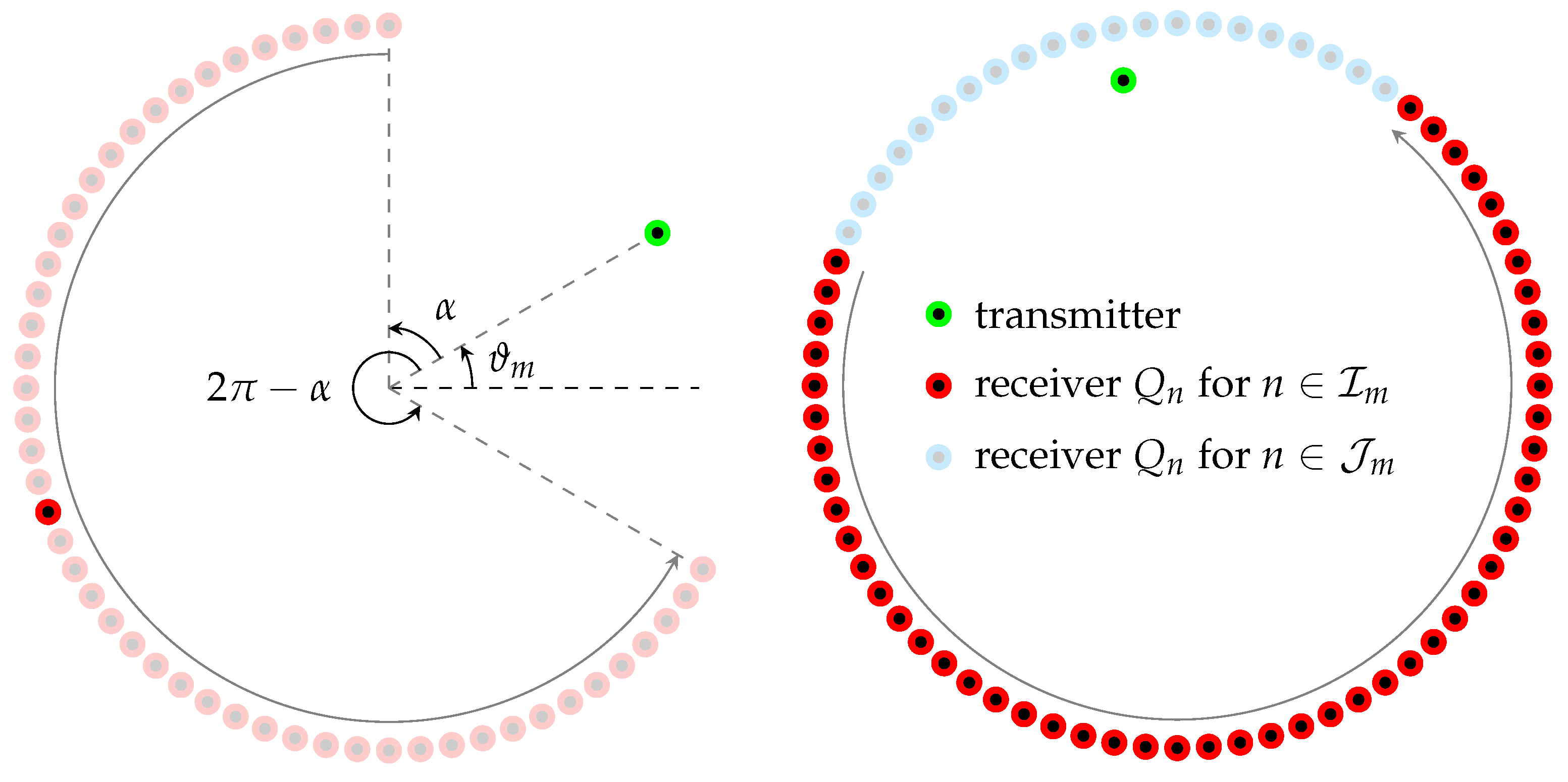
In this study, a bistatic measurement system is considered. Here, when a transmitter is fixed, the receiver rotates while measuring the data (as shown in Figure 1). To describe the measurement configuration, ${\mathcal{P}}_m$ and ${\mathcal{Q}}_n$ denote the mth transmitter and nth receiver, respectively. In addition, ${\mathbf{p}}_m$ and ${\mathbf{q}}_n$ denote the locations of ${\mathcal{P}}_m$ and ${\mathcal{Q}}_n$, respectively, such that

$${\mathbf{p}}_m=P{\mathit{\vartheta }}_m=P(cos{\vartheta }_m,sin{\vartheta }_m)\mathrm{and}{\mathbf{q}}_n=Q{\mathit{\theta }}_n=Q(cos{\theta }_n,sin{\theta }_n),$$

where for $m=1,2,\dots ,M$ and $n=1,2,\dots ,N$

$${\vartheta }_m=(m-1)▵\vartheta ={\displaystyle \frac{2\pi (m-1)}{M}}\mathrm{and}{\theta }_n=(n-1)▵\theta ={\displaystyle \frac{2\pi (n-1)}{N}}.$$

Furthermore, $\mathcal{P}$ and $\mathcal{Q}$ denote the collection of transmitters ${\mathcal{P}}_m$ and receivers ${\mathcal{Q}}_n$, respectively.

Figure 1. Bistatic measurement system.

Remark 1.

Here, we provide a detailed discussion of several conditions.

1. 

(Smallness of an object) If ${\alpha }_m$ satisfies

$$\left(\sqrt{{\displaystyle \frac{{\epsilon }_s}{{\epsilon }_0}}}-1\right){\alpha }_m<{\displaystyle \frac{\lambda }{4}},$$

then, following [43], the object $D_s$ can be regarded as small, and the approximation in (2) can be applied.

2. 

(Well separation of objects) We let $d(s,s^{\prime })=dist(D_s,D_{s^{\prime }})$ be the distance between two objects $D_s$ and $D_{s^{\prime }}$ providing $s\ne s^{\prime }$. If $d(s,s^{\prime })$ satisfies

$$d(s,s^{\prime })>{\displaystyle \frac{2.4048}{k}}\mathit{for}\mathit{all}s,s^{\prime }=1,2,\dots ,S,$$

then, following [44], all the objects can be assumed to be well-separated. Here, $2.4048$ is the first zero of the Bessel function of order zero. Note that in the three-dimensional problem, the condition is $d(s,s^{\prime })>\lambda /2$.

3. 

(Number of transmitters and receivers) We let R denote the radius of a circular imaging region. If

$$N,M>4kR$$

(1)

then, following [45], it can be ensured that good imaging results are obtained. Since $M=36$ and $N=72$ in Fresnel experimental dataset [39], we select $f=4\mathrm{GHz}$ ($k\approx 83.8338$) and $R=0.1 \mathrm{m}$ in Section 5 to satisfy Condition (1).

In this paper, we denote $u(\mathbf{r},{\mathbf{p}}_m)$ as the time-harmonic total field, which is the z-component of the electric field and satisfies the scalar Helmholtz equation in the presence of D

$$▵u(\mathbf{r},{\mathbf{p}}_m)+{\omega }^2\epsilon \left(\mathbf{r}\right){\mu }_{0}u(\mathbf{r},{\mathbf{p}}_m)=0,\mathbf{r}\in \Omega$$

with transmission condition at $\partial D_s$. We refer to [12,15,39] for a detailed description. The incident field $u_0(\mathbf{r},{\mathbf{p}}_m)$ generated at ${\mathcal{P}}_m$ satisfies the following equation:

$$▵u_0(\mathbf{r},{\mathbf{p}}_m)+k^2{u}_0(\mathbf{r},{\mathbf{p}}_m)=0,\mathbf{r}\in \Omega .$$

Here, the time harmonic dependence $e^{-i\omega t}$ is assumed, $k^2$ is not an eigenvalue for the operator $-▵$, and

$$u_0(\mathbf{r},{\mathbf{r}}^{\prime })=G(\mathbf{r},{\mathbf{r}}^{\prime })=-{\displaystyle \frac{i}{4}}{H}_0^{\left(1\right)}\left(k\right|\mathbf{r}-{\mathbf{r}}^{\prime }\left|\right),\mathbf{r}\ne {\mathbf{r}}^{\prime },$$

where $H_0^{\left(1\right)}$ denotes the zero order Hankel function of the first kind. $u_{scat}({\mathbf{q}}_n,{\mathbf{p}}_m)$ denotes the scattered field measured at the ${\mathcal{Q}}_n$ corresponding to the incident field that satisfies $u_{scat}({\mathbf{q}}_n,{\mathbf{p}}_m)=u({\mathbf{q}}_n,{\mathbf{p}}_m)-u_0({\mathbf{q}}_n,{\mathbf{p}}_m)$ and the Sommerfeld radiation condition:

$$\underset{\left|\mathbf{r}\right|\to \infty }{lim}\sqrt{\left|\mathbf{r}\right|}\left({\displaystyle \frac{\partial u_{scat}(\mathbf{r},{\mathbf{p}}_m)}{\partial \left|\mathbf{r}\right|}}-ik{u}_{scat}(\mathbf{r},{\mathbf{p}}_m)\right)=0\mathrm{uniformly}\mathrm{in}\mathrm{all}\mathrm{directions}{\displaystyle \frac{\mathbf{r}}{\left|\mathbf{r}\right|}}.$$

Note that a complete expression of $u_{scat}({\mathbf{q}}_n,{\mathbf{p}}_m)$ is required to design an indicator function for the DSM. To this end, based on the findings of a previous study [13], we adopt the following approximation:

$$u_{scat}({\mathbf{q}}_n,{\mathbf{p}}_m)\approx k^2{\int }_D\mathcal{O}\left({\mathbf{r}}^{\prime }\right)G({\mathbf{q}}_n,{\mathbf{r}}^{\prime })G({\mathbf{r}}^{\prime },{\mathbf{p}}_m)\mathrm{d}{\mathbf{r}}^{\prime },\mathcal{O}\left({\mathbf{r}}^{\prime }\right)={\displaystyle \frac{\epsilon \left({\mathbf{r}}^{\prime }\right)-{\epsilon }_0}{{\epsilon }_0{\mu }_0}}.$$

(2)

3. Indicator Function of the DSM with a Single Source

3.1. Introduction of the Indicator Function

Here, we introduce the indicator function of the DSM with a single source. For a fixed transmitter ${\mathcal{P}}_m$, we generate an arrangement of the measurement data such that

$$\mathbb{S}\left(m\right)=\left[\begin{array}{c}{u}_{scat}({\mathbf{q}}_1,{\mathbf{p}}_m)\\ u_{scat}({\mathbf{q}}_2,{\mathbf{p}}_m)\\ ⋮\\ u_{scat}({\mathbf{q}}_N,{\mathbf{p}}_m)\end{array}\right].$$

(3)

By applying the mean-value theorem to (2), $u_{scat}({\mathbf{q}}_n,{\mathbf{p}}_m)$ can be approximated as follows:

$$u_{scat}({\mathbf{q}}_n,{\mathbf{p}}_m)\approx k^2\sum _{s=1}^S\left({\displaystyle \frac{{\epsilon }_s-{\epsilon }_0}{{\epsilon }_0{\mu }_0}}\right)area\left(D_s\right)G({\mathbf{p}}_m,{\mathbf{r}}_s)G({\mathbf{q}}_n,{\mathbf{r}}_s),$$

(4)

where $area\left(D_s\right)$ denotes the area of $D_s$. Correspondingly, $\mathbb{S}\left(m\right)$ is approximated as

$$\begin{array}{cc}\hfill \mathbb{S}\left(m\right)& \approx k^2{\displaystyle \sum _{s=1}^S}\left({\displaystyle \frac{{\epsilon }_s-{\epsilon }_0}{{\epsilon }_0{\mu }_0}}\right)area\left(D_s\right)G({\mathbf{p}}_m,{\mathbf{r}}_s)\left[\begin{array}{c}G({\mathbf{q}}_1,{\mathbf{r}}_s)\\ G({\mathbf{q}}_2,{\mathbf{r}}_s)\\ ⋮\\ G({\mathbf{q}}_N,{\mathbf{r}}_s)\end{array}\right]\hfill \\ \hfill & :=k^2{\displaystyle \sum _{s=1}^S}\left({\displaystyle \frac{{\epsilon }_s-{\epsilon }_0}{{\epsilon }_0{\mu }_0}}\right)area\left(D_s\right)G({\mathbf{p}}_m,{\mathbf{r}}_s)\mathbb{G}\left({\mathbf{r}}_s\right).\hfill \end{array}$$

Based on the above expression, we generate a test vector corresponding to the receivers. Here, for each search point $\mathbf{r}\in \Omega$, we generate

$$\mathbb{Q}\left(\mathbf{r}\right)=\left[\begin{array}{c}G({\mathbf{q}}_1,\mathbf{r})\\ G({\mathbf{q}}_2,\mathbf{r})\\ ⋮\\ G({\mathbf{q}}_N,\mathbf{r})\end{array}\right].$$

(5)

Based on the orthogonality property of the Hilbert space ${\ell }^2$, the value

$${⟨\mathbb{G}\left({\mathbf{r}}_s\right),\mathbb{Q}\left(\mathbf{r}\right)⟩}_{{\ell }^2\left(\mathcal{Q}\right)}:=\mathbb{G}\left({\mathbf{r}}_s\right)·\overline{\mathbb{Q}\left(\mathbf{r}\right)}=\sum _{n=1}^{N}G({\mathbf{q}}_n,{\mathbf{r}}_s)\overline{G({\mathbf{q}}_n,\mathbf{r})}$$

(6)

will reach its maximum value when $\mathbf{r}={\mathbf{r}}_s\in D_s$. Correspondingly, by defining the norm ${\parallel ·\parallel }_{{\ell }^2\left(\mathcal{Q}\right)}={⟨·,·⟩}_{{\ell }^2\left(\mathcal{Q}\right)}^{1/2}$, the following classical indicator function of the DSM can be introduced: for each search point $\mathbf{r}\in \Omega$,

$$\mathfrak{F}(\mathbf{r},m)={\displaystyle \frac{\left|{⟨\mathbb{S}\left(m\right),\mathbb{Q}\left(\mathbf{r}\right)⟩}_{{\ell }^2\left(\mathcal{Q}\right)}\right|}{{\parallel \mathbb{S}\left(m\right)\parallel }_{{\ell }^2\left(\mathcal{Q}\right)}{\parallel \mathbb{Q}\left(\mathbf{r}\right)\parallel }_{{\ell }^2\left(\mathcal{Q}\right)}}}.$$

(7)

Then, $\mathfrak{F}(\mathbf{r},m)\approx 1$ when $\mathbf{r}={\mathbf{r}}_s\in D_s$, $s=1,2,\dots ,S$; thus, by regarding peaks of large magnitudes in the map of $\mathfrak{F}(\mathbf{r},m)$, it is possible to identify the objects $D_s$. Refer to the literature [24,26] for a more detailed description.

However, $u_{scat}({\mathbf{q}}_n,{\mathbf{p}}_m)$ cannot be expressed as (2) due to the interference between the antennas because using the classical indicator function in (7) in this case is nonsense. To avoid such interference, when a transmitter is placed at a fixed position ${\mathbf{p}}_m$, a receiver is rotating within the range ${\vartheta }_m+\alpha$ to ${\vartheta }_m+2\pi -\alpha$ for $0<\alpha <\pi$ (in [39], the value of $\alpha$ is set to $60°$), as shown in Figure 1. Here, $\alpha$ denotes the minimum bistatic angle, i.e., the angle between the transmitter and the receiver. This means that the complete elements of $\mathbb{S}\left(m\right)$ of (3) cannot be used to design the indicator function in (7). Now, we define the following two index sets:

$$\begin{array}{cc}\hfill \mathcal{I}\left(m\right)& =\left\{n:{\vartheta }_m+\alpha \le {\theta }_n\le {\vartheta }_m+2\pi -\alpha \right\},\hfill \\ \hfill \mathcal{J}\left(m\right)& =\left\{n:{\vartheta }_m-\alpha <{\theta }_n<{\vartheta }_m+\alpha \right\}=\left\{1,2,\dots ,N\right\}\setminus \mathcal{I}\left(m\right).\hfill \end{array}$$

Then, it is possible to collect $u_{scat}({\mathbf{q}}_n,{\mathbf{p}}_m)$ for $n\in \mathcal{I}\left(m\right)$. In most studies, the unmeasurable scattered field data were set to zero because there was no signal reception at the receiving antenna ${\mathcal{Q}}_n$ for $n\in \mathcal{J}\left(m\right)$. See [40,41,42] for related works. In contrast to previous studies, we generate an arrangement of measurement data by converting uncollectible data to a fixed constant C such that

$$\mathbb{S}(C,m)=\left[a_{nm}\right]\in {\mathbb{C}}^{N\times 1},\mathrm{where}{a}_{nm}=\left\{\begin{array}{cc}{u}_{scat}({\mathbf{q}}_n,{\mathbf{p}}_m),& n\in \mathcal{I}\left(m\right)\hfill \\ C,& n\in \mathcal{J}\left(m\right).\hfill \end{array}\right.$$

With this, we introduce the following indicator function of the DSM corresponding to the fixed transmitter ${\mathcal{P}}_m$: for each search point $\mathbf{r}\in \Omega$ and fixed constant C,

$${\mathfrak{F}}_{DSM}(\mathbf{r},m,C)={\displaystyle \frac{\left|{|⟨\mathbb{S}(C,m),\mathbb{Q}\left(\mathbf{r}\right)⟩}_{{\ell }^2\left(\mathcal{Q}\right)}\right|}{{\parallel \mathbb{S}(C,m)\parallel }_{{\ell }^2\left(\mathcal{Q}\right)}{\parallel \mathbb{Q}\left(\mathbf{r}\right)\parallel }_{{\ell }^2\left(\mathcal{Q}\right)}}}.$$

(8)

Note that the test vector $\mathbb{Q}\left(\mathbf{r}\right)$ is given in (5).

3.2. Mathematical Structure of the Indicator Function

Throughout the numerical simulation results discussed in Section 5, the imaging performance is strongly dependent on the location of ${\mathcal{P}}_m$ and the value of C. To explain this phenomenon theoretically, we investigate the mathematical structure of the indicator function as follows.

Theorem 1.

Here, we assume that $4k|\mathbf{r}-{\mathbf{q}}_n|\gg 1$ for all $\mathbf{r}\in \Omega$ and $n=1,2,\dots ,N$. Then, ${\mathfrak{F}}_{DSM}(\mathbf{r},m,C)$ can be approximated as follows:

$${\mathfrak{F}}_{DSM}(\mathbf{r},m,C)\approx {\displaystyle \frac{|\Phi \left(\mathbf{r}\right)+\Psi (\mathbf{r},m,C)|}{{\displaystyle \underset{\mathbf{r}\in \Omega }{max}|\Phi \left(\mathbf{r}\right)+\Psi (\mathbf{r},m,C)|}}},$$

(9)

where

$$\Phi \left(\mathbf{r}\right)={\displaystyle \frac{k^2\#\left[\mathcal{I}\left(m\right)\right]}{2\sqrt{kQ\pi }}}{\int }_D\mathcal{O}\left({\mathbf{r}}^{\prime }\right)G({\mathbf{p}}_m,{\mathbf{r}}^{\prime })\left(J_0\left(k\right|\mathbf{r}-{\mathbf{r}}^{\prime }\left|\right)+{\mathcal{E}}_1(\mathbf{r},{\mathbf{r}}^{\prime },m)\right)\mathrm{d}{\mathbf{r}}^{\prime }$$

(10)

and

$$\Psi (\mathbf{r},m,C)=-C(1+i)\#\left[\mathcal{J}\left(m\right)\right]\left(J_0\left(k\right|\mathbf{r}\left|\right)+{\mathcal{E}}_2(\mathbf{r},m)\right).$$

Here, $\#\left[\mathcal{I}\right(m\left)\right]$ denotes the number of elements in the set $\mathcal{I}\left(m\right)$, and $J_n$ is the Bessel function of order n. In addition, we obtain the following:

$$\begin{array}{c}\hfill \begin{array}{cc}\hfill & {\mathcal{E}}_1(\mathbf{r},{\mathbf{r}}^{\prime },m)=2{\displaystyle \sum _{p=1}^{\infty }}{i}^p{J}_p\left(k\right|\mathbf{r}-{\mathbf{r}}^{\prime }\left|\right)cos\left(p({\vartheta }_m-\varphi )\right)sinc\left(p(\pi -\alpha )\right)\hfill \\ \hfill & {\mathcal{E}}_2(\mathbf{r},m)=2{\displaystyle \sum _{q=1}^{\infty }}{i}^q{J}_q\left(k\right|\mathbf{r}\left|\right)cos\left(q({\vartheta }_m-\psi )\right)sinc\left(q\alpha \right),\hfill \end{array}\end{array}$$

(11)

where $sinc\left(x\right)$ denotes the unnormalized sinc function defined for $x\ne 0$ by

$$sinc\left(x\right)={\displaystyle \frac{sinx}{x}}.$$

Proof. 

Since $4k|\mathbf{r}-{\mathbf{q}}_n|\gg 1$ for all n, the following asymptotic form holds (refer to the [15] for additional information):

$$-{\displaystyle \frac{i}{4}}{H}_0^{\left(1\right)}\left(k\right|\mathbf{r}-{\mathbf{q}}_n\left|\right)=-{\displaystyle \frac{(1+i)e^{ikQ}}{4\sqrt{kQ\pi }}}{e}^{-ik{\mathit{\theta }}_n·\mathbf{r}}.$$

(12)

Then, since

$$\mathbb{Q}\left(\mathbf{r}\right)=-{\displaystyle \frac{(1+i)e^{-ikQ}}{4\sqrt{kQ\pi }}}\left[\begin{array}{c}{e}^{-ik{\mathit{\theta }}_1·\mathbf{r}}\\ e^{-ik{\mathit{\theta }}_2·\mathbf{r}}\\ ⋮\\ e^{-ik{\mathit{\theta }}_N·\mathbf{r}}\end{array}\right]$$

and based on (2)

$$u_{scat}({\mathbf{q}}_n,{\mathbf{p}}_m)=-{\displaystyle \frac{k^2(1+i)e^{ikQ}}{4\sqrt{kQ\pi }}}{\int }_D\mathcal{O}\left({\mathbf{r}}^{\prime }\right)G({\mathbf{r}}^{\prime },{\mathbf{p}}_m)e^{-ik{\mathit{\theta }}_n·{\mathbf{r}}^{\prime }}\mathrm{d}{\mathbf{r}}^{\prime },$$

we can evaluate the following:

$$\begin{array}{cc}\hfill {⟨\mathbb{S}(C,m),\mathbb{Q}\left(\mathbf{r}\right)⟩}_{{\ell }^2\left(\mathcal{Q}\right)}=& {\displaystyle \frac{i{k}^2}{8kQ\pi }}{\int }_D\mathcal{O}\left({\mathbf{r}}^{\prime }\right)G({\mathbf{r}}^{\prime },{\mathbf{p}}_m){\displaystyle \sum _{n\in \mathcal{I}\left(m\right)}}{e}^{ik{\mathit{\theta }}_n·(\mathbf{r}-{\mathbf{r}}^{\prime })}\mathrm{d}{\mathbf{r}}^{\prime }\hfill \\ \hfill & -{\displaystyle \frac{C(1+i)e^{-ikQ}}{4\sqrt{kQ\pi }}}{\displaystyle \sum _{n\in \mathcal{J}\left(m\right)}}{e}^{ik{\mathit{\theta }}_n·\mathbf{r}}\hfill \end{array}$$

The following relation holds uniformly (refer to the literature [37] for the derivation).

$$\begin{array}{c}\hfill \begin{array}{cc}\hfill & {\displaystyle \sum _{n=1}^N}{e}^{ixcos({\theta }_n-\varphi )}={\displaystyle \frac{N}{N▵\theta }}{\displaystyle \sum _{n=1}^N}{e}^{ixcos({\theta }_n-\varphi )}▵\theta \approx {\displaystyle \frac{N}{{\theta }_N-{\theta }_1}}{\int }_{{\theta }_1}^{{\theta }_N}{e}^{ixcos(\theta -\varphi )}\mathrm{d}\theta \hfill \\ \hfill & =N\left(J_0\left(x\right)+{\displaystyle \frac{4}{{\theta }_N-{\theta }_1}}{\displaystyle \sum _{p=1}^{\infty }}{\displaystyle \frac{i^p}{p}}{J}_p\left(x\right)cos{\displaystyle \frac{p({\theta }_N+{\theta }_1-2\varphi )}{2}}sin{\displaystyle \frac{p({\theta }_N-{\theta }_1)}{2}}\right)\hfill \\ \hfill & =N\left(J_0\left(x\right)+2{\displaystyle \sum _{p=1}^{\infty }}{i}^p{J}_p\left(x\right)cos{\displaystyle \frac{p({\theta }_N+{\theta }_1-2\varphi )}{2}}sinc\left(p({\theta }_N-{\theta }_1)\right)\right).\hfill \end{array}\end{array}$$

(13)

Thus, by letting $\mathbf{r}-{\mathbf{r}}^{\prime }=|\mathbf{r}-{\mathbf{r}}^{\prime }|(cos\varphi ,sin\varphi )$ and $\mathbf{r}=\left|\mathbf{r}\right|(cos\psi ,sin\psi )$, we can evaluate

$$\begin{array}{cc}\hfill {\displaystyle \sum _{n\in \mathcal{I}\left(m\right)}}& e^{ik{\mathit{\theta }}_n·(\mathbf{r}-{\mathbf{r}}^{\prime })}={\displaystyle \frac{\#\left[\mathcal{I}\right(m\left)\right]}{\#\left[\mathcal{I}\right(m\left)\right]▵\theta }}{\displaystyle \sum _{n\in \mathcal{I}\left(m\right)}}{e}^{ik{\mathit{\theta }}_n·(\mathbf{r}-{\mathbf{r}}^{\prime })}▵\theta \hfill \\ \hfill & \approx {\displaystyle \frac{\#\left[\mathcal{I}\right(m\left)\right]}{2\pi -2\alpha }}{\int }_{{\vartheta }_m+\alpha }^{{\vartheta }_m+2\pi -\alpha }{e}^{ik|\mathbf{r}-{\mathbf{r}}^{\prime }|cos(\theta -\varphi )}\mathrm{d}\theta \hfill \\ \hfill & =\#\left[\mathcal{I}\left(m\right)\right]\left[J_0\left(k\right|\mathbf{r}-{\mathbf{r}}^{\prime }\left|\right)+{\displaystyle \frac{2}{\pi -\alpha }}{\displaystyle \sum _{p=1}^{\infty }}{\displaystyle \frac{i^p}{p}}{J}_p\left(k\right|\mathbf{r}-{\mathbf{r}}^{\prime }\left|\right)cos\left(p({\vartheta }_m-\varphi )\right)sin\left(p(\pi -\alpha )\right)\right]\hfill \\ \hfill & =\#\left[\mathcal{I}\left(m\right)\right]\left[J_0\left(k\right|\mathbf{r}-{\mathbf{r}}^{\prime }\left|\right)+2{\displaystyle \sum _{p=1}^{\infty }}{i}^p{J}_p\left(k\right|\mathbf{r}-{\mathbf{r}}^{\prime }\left|\right)cos\left(p({\vartheta }_m-\varphi )\right){\displaystyle \frac{sin\left(p(\pi -\alpha )\right)}{p(\pi -\alpha )}}\right]\hfill \end{array}$$

and

$$\begin{array}{cc}\hfill {\displaystyle \sum _{n\in \mathcal{J}\left(m\right)}}{e}^{ik{\mathit{\theta }}_n·\mathbf{r}}& ={\displaystyle \frac{\#\left[\mathcal{J}\right(m\left)\right]}{\#\left[\mathcal{J}\right(m\left)\right]▵\theta }}{\displaystyle \sum _{n\in \mathcal{J}\left(m\right)}}{e}^{ik{\mathit{\theta }}_n·\mathbf{r}}▵\theta \approx {\displaystyle \frac{\#\left[\mathcal{J}\right(m\left)\right]}{2\alpha }}{\int }_{{\vartheta }_m-\alpha }^{{\vartheta }_m+\alpha }{e}^{ik\left|\mathbf{r}\right|cos(\theta -\psi )}\mathrm{d}\theta \hfill \\ \hfill & =\#\left[\mathcal{J}\left(m\right)\right]\left[J_0\left(k\right|\mathbf{r}\left|\right)+{\displaystyle \frac{2}{\alpha }}{\displaystyle \sum _{q=1}^{\infty }}{\displaystyle \frac{i^q}{q}}{J}_q\left(k\right|\mathbf{r}\left|\right)cos\left(q({\vartheta }_m-\psi )\right)sin\left(q\alpha \right)\right]\hfill \\ \hfill & =\#\left[\mathcal{J}\left(m\right)\right]\left[J_0\left(k\right|\mathbf{r}\left|\right)+2{\displaystyle \sum _{q=1}^{\infty }}{i}^q{J}_q\left(k\right|\mathbf{r}\left|\right)cos\left(q({\vartheta }_m-\psi )\right){\displaystyle \frac{sin\left(q\alpha \right)}{q\alpha }}\right].\hfill \end{array}$$

Therefore, we can derive

$$\begin{array}{c}{⟨\mathbb{S}(C,m),\mathbb{Q}\left(\mathbf{r}\right)⟩}_{{\ell }^2\left(\mathcal{Q}\right)}={\displaystyle \frac{i{k}^2\#\left[\mathcal{I}\left(m\right)\right]}{8kQ\pi }}{\int }_D\mathcal{O}\left({\mathbf{r}}^{\prime }\right)G({\mathbf{r}}^{\prime },{\mathbf{p}}_m)\left(J_0\left(k\right|\mathbf{r}-{\mathbf{r}}^{\prime }\left|\right)+{\mathcal{E}}_1(\mathbf{r},{\mathbf{r}}^{\prime },m)\right)\mathrm{d}{\mathbf{r}}^{\prime }\hfill \\ \hfill -{\displaystyle \frac{C(1+i)\#\left[\mathcal{J}\left(m\right)\right]e^{-ikQ}}{4\sqrt{kQ\pi }}}\left(J_0\left(k\right|\mathbf{r}\left|\right)+{\mathcal{E}}_2(\mathbf{r},m)\right).\end{array}$$

(14)

Finally, the approximation given in (9) can be obtained by applying Hölder’s inequality as follows:

$${⟨\mathbb{S}(C,m),\mathbb{Q}\left(\mathbf{r}\right)⟩}_{{\ell }^2\left(\mathcal{Q}\right)}\le {\parallel \mathbb{S}(C,m)\parallel }_{{\ell }^2\left(\mathcal{Q}\right)}{\parallel \mathbb{Q}\left(\mathbf{r}\right)\parallel }_{{\ell }^2\left(\mathcal{Q}\right)}.$$

   □

3.3. Properties of Indicator Function with a Single Source

Based on Theorem 1, we discuss some properties of the indicator function with a single source.

Discussion 1

(Composition of Indicator Function). Since $J_0\left(0\right)=1$ and $J_p\left(0\right)=0$ for $p\ne 0$, the factor $J_0\left(k\right|\mathbf{r}-{\mathbf{r}}^{\prime }\left|\right)$ contributes to the object detection because $J_0\left(k\right|\mathbf{r}-{\mathbf{r}}^{\prime }\left|\right)=1$ when $\mathbf{r}={\mathbf{r}}^{\prime }\in D$. However, due to the factor $G({\mathbf{p}}_m,{\mathbf{r}}^{\prime })$, the imaging performance is strongly dependent on the location of the transmitter. In contrast, the factor ${\mathcal{E}}_1(\mathbf{r},{\mathbf{r}}^{\prime },m)$ disturbs the object detection because ${\mathcal{E}}_1(\mathbf{r},{\mathbf{r}}^{\prime },m)=0$ when $\mathbf{r}={\mathbf{r}}^{\prime }\in D$ and generates several artifacts based on the oscillation property of the Bessel function. In addition, due to the factor $J_0\left(k\right|\mathbf{r}\left|\right)$, a peak of large magnitude will appear at the origin, which disturbs the object detection (unless the object is located at the origin). Finally, the factor ${\mathcal{E}}_2(\mathbf{r},m)$ generates several artifacts and does not contribute to the object detection.

Discussion 2

(Influence of Bistatic Angle). Based on (9), we can observe that the imaging performance of ${\mathfrak{F}}_{DSM}(\mathbf{r},m,C)$ is strongly dependent on $\alpha$. If $\alpha$ is sufficiently small such that  $\alpha ⟶0+$, then since $\#\left[\mathcal{J}\right(m\left)\right]⟶0+$ and $sinc\left(p\pi \right)=0$ for any integer p,

$$\underset{\alpha \to 0+}{lim}{\mathcal{E}}_1(\mathbf{r},{\mathbf{r}}^{\prime },m)=2\sum _{p=1}^{\infty }{i}^p{J}_p\left(k\right|\mathbf{r}-{\mathbf{r}}^{\prime }\left|\right)cos\left(p({\vartheta }_m-\varphi )\right)\left(\underset{\alpha \to 0+}{lim}sinc\left(p(\pi -\alpha )\right)\right)=0,$$

the factor $\Phi \left(\mathbf{r}\right)$ becomes

$$\Phi \left(\mathbf{r}\right)={\displaystyle \frac{k^2\#\left[\mathcal{I}\left(m\right)\right]}{2\sqrt{kQ\pi }}}{\int }_D\mathcal{O}\left({\mathbf{r}}^{\prime }\right)G({\mathbf{p}}_m,{\mathbf{r}}^{\prime })J_0\left(k\right|\mathbf{r}-{\mathbf{r}}^{\prime }\left|\right)\mathrm{d}{\mathbf{r}}^{\prime }.$$

Thus, a good imaging result is expected when $\alpha$ is small because the disturbing factors are eliminated. Otherwise, if $\alpha ⟶\pi -$, then since

$$\underset{\alpha \to \pi -}{lim}sinc\left(p(\pi -\alpha )\right)=1,$$

based on the uniform convergence of the Jacobi–Anger expansion formula (refer to the literature [15] for additional details)

$$e^{ixcos\vartheta }=J_0\left(x\right)+2\sum _{p=1}^{\infty }{i}^p{J}_p\left(x\right)cos\left(p\vartheta \right),$$

(15)

we obtain

$$J_0\left(k\right|\mathbf{r}-{\mathbf{r}}^{\prime }\left|\right)+2\sum _{p=1}^{\infty }{i}^p{J}_p\left(k\right|\mathbf{r}-{\mathbf{r}}^{\prime }\left|\right)cos\left(p({\vartheta }_m-\varphi )\right)=e^{ik|\mathbf{r}-{\mathbf{r}}^{\prime }|cos({\vartheta }_m-\varphi )}=e^{ik{\vartheta }_m·(\mathbf{r}-{\mathbf{r}}^{\prime })}$$

and correspondingly, the factor $\Phi \left(\mathbf{r}\right)$ in (9) becomes

$$\begin{array}{cc}\hfill \Phi \left(\mathbf{r}\right)& ={\displaystyle \frac{k^2\#\left[\mathcal{I}\left(m\right)\right]}{2\sqrt{kQ\pi }}}{\int }_D\mathcal{O}\left({\mathbf{r}}^{\prime }\right)G({\mathbf{p}}_m,{\mathbf{r}}^{\prime })e^{ik{\vartheta }_m·(\mathbf{r}-{\mathbf{r}}^{\prime })}\mathrm{d}{\mathbf{r}}^{\prime }.\hfill \end{array}$$

In addition, since $\left|e^{ik{\vartheta }_m·(\mathbf{r}-{\mathbf{r}}^{\prime })}\right|\equiv 1$ for every $\mathbf{r}\in \Omega$, the factor $\Phi \left(\mathbf{r}\right)$ ceases to contribute to the identification of the objects D, but instead plays a role in imaging the source location under the influence of $G({\mathbf{p}}_m,{\mathbf{r}}^{\prime })$. Consequently, it is impossible to identify the objects through the map ${\mathfrak{F}}_{DSM}(\mathbf{r},m,C)$ when $\alpha$ is close to $\pi$.

Discussion 3

(Influence of Converted Constant). Here, we assume that $0<\alpha <\pi$ and $\mathbf{r}={\mathbf{r}}_s\in D_s$ for some s. Then, based on Discussion 1,

$$\Phi \left(\mathbf{r}\right)={\displaystyle \frac{k^2\#\left[\mathcal{I}\left(m\right)\right]}{2\sqrt{kQ\pi }}}{\int }_{D_s}\left({\displaystyle \frac{{\epsilon }_s-{\epsilon }_0}{{\epsilon }_0{\mu }_0}}\right)G({\mathbf{p}}_m,{\mathbf{r}}^{\prime })\mathrm{d}{\mathbf{r}}^{\prime }-C(1+i)\#\left[\mathcal{J}\left(m\right)\right]\left(J_0\left(k\right|\mathbf{r}\left|\right)+{\mathcal{E}}_2(\mathbf{r},m)\right).$$

Thus, if C satisfies

$$\left|C\right|\ll {\displaystyle \frac{k^2\#\left[\mathcal{I}\left(m\right)\right]}{2\#\left[\mathcal{J}\left(m\right)\right]\sqrt{2kQ\pi }}}\left({\displaystyle \frac{{\epsilon }_s-{\epsilon }_0}{{\epsilon }_0{\mu }_0}}\right){\displaystyle \frac{G({\mathbf{p}}_m,{\mathbf{r}}_s)area\left(D_s\right)}{J_0\left(k\right|{\mathbf{r}}_s\left|\right)+{\mathcal{E}}_2({\mathbf{r}}_s,m)}},$$

then the factor $\left|\Psi (\mathbf{r},m,C)\right|$ is dominated by $\left|\Phi \left(\mathbf{r}\right)\right|$. As a result, it is possible to recognize $D_s$ through the map of ${\mathfrak{F}}_{DSM}(\mathbf{r},m,C)$. Otherwise, if C satisfies the following relation for all $s=1,2,\dots ,S$,

$$\left|C\right|\gg {\displaystyle \frac{k^2\#\left[\mathcal{I}\left(m\right)\right]}{2\#\left[\mathcal{J}\left(m\right)\right]\sqrt{2kQ\pi }}}\left({\displaystyle \frac{{\epsilon }_s-{\epsilon }_0}{{\epsilon }_0{\mu }_0}}\right){\displaystyle \frac{G({\mathbf{p}}_m,{\mathbf{r}}_s)area\left(D_s\right)}{J_0\left(k\right|{\mathbf{r}}_s\left|\right)+{\mathcal{E}}_2({\mathbf{r}}_s,m)}},$$

then the factor $\left|\Phi \left(\mathbf{r}\right)\right|$ is dominated by $\left|\Psi (\mathbf{r},m,C)\right|$. This means that the map of ${\mathfrak{F}}_{DSM}(\mathbf{r},m,C)$ only contains a peak of large magnitude at the origin. Thus, it is very difficult to recognize the existence, location, and shape of the objects.

Based on the above observations, the selection of C to identify $D_s$ is highly dependent on the ${\epsilon }_s$ values, the size of $D_s$, k, and the total number of transmitting and receiving antennas.

Discussion 4

(Best Choice for the Constant). Based on both Discussions 2 and 3, $C=0$ and $\alpha ⟶0$ guarantee good imaging results. However, the setting $\alpha ⟶0$ is impossible; thus, $C=0$ is the best choice for a proper application of the designed DSM, which is the theoretical rationale for converting unmeasurable data to zero in previous studies.

Discussion 5

(Dependence of Material Properties). If $C=0$ and $\mathbf{r}\in D$ then based on (9),

$$\left|\Phi \left(\mathbf{r}\right)\right|\propto \left|{\int }_D\mathcal{O}\left({\mathbf{r}}^{\prime }\right)G({\mathbf{p}}_m,{\mathbf{r}}^{\prime })\mathrm{d}{\mathbf{r}}^{\prime }\right|=\left|{\int }_D\left({\displaystyle \frac{\epsilon \left({\mathbf{r}}^{\prime }\right)-{\epsilon }_0}{{\epsilon }_0{\mu }_0}}\right)G({\mathbf{p}}_m,{\mathbf{r}}^{\prime })\mathrm{d}{\mathbf{r}}^{\prime }\right|,$$

the value of ${\mathfrak{F}}_{DSM}(\mathbf{r},m,0)$ depends on the material properties (size and permittivity) of objects. For example, suppose there exist two objects $D_1$ and $D_2$ of the same size but with different permittivities ${\epsilon }_1$ and ${\epsilon }_2$, where ${\epsilon }_1>{\epsilon }_2$. In this case, ${\mathfrak{F}}_{DSM}({\mathbf{r}}_1,m,0)>{\mathfrak{F}}_{DSM}({\mathbf{r}}_2,m,0)$, i.e., $D_1$ is more clearly visible than $D_2$ through the map of ${\mathfrak{F}}_{DSM}(\mathbf{r},m,0)$. A similar phenomenon can also be observed when ${\epsilon }_1={\epsilon }_2$ and $area\left(D_1\right)>area\left(D_2\right)$ are considered.

4. Indicator Function of DSM with Multiple Sources

Further improvement of the indicator with a single source is required because the imaging performance is strongly dependent on the location of the transmitter (refer to Discussion 1) and the selection of the constant C, which is in turn highly dependent on the given problem at hand (e.g., the material properties of unknown objects; refer to Discussion 3). Thus, in the following, we introduce an indicator function with multiple sources.

4.1. Introduction of the Indicator Function

For each transmitter ${\mathcal{P}}_m$, $m=1,2,\dots ,M$, we generate an arrangement such that

$$\mathbb{M}\left(C\right)=\left[\begin{array}{c}{⟨\mathbb{M}(C,1),\mathbb{Q}\left(\mathbf{r}\right)⟩}_{{\ell }^2\left(\mathcal{Q}\right)}\\ {⟨\mathbb{M}(C,2),\mathbb{Q}\left(\mathbf{r}\right)⟩}_{{\ell }^2\left(\mathcal{Q}\right)}\\ ⋮\\ {⟨\mathbb{S}(C,M),\mathbb{Q}\left(\mathbf{r}\right)⟩}_{{\ell }^2\left(\mathcal{Q}\right)}\end{array}\right].$$

Here, if $C=0$, since $\#\left[\mathcal{I}\right(m\left)\right]$ are identical, then based on (14),

$${⟨\mathbb{M}(0,m),\mathbb{Q}\left(\mathbf{r}\right)⟩}_{{\ell }^2\left(\mathcal{Q}\right)}={\displaystyle \frac{i{k}^2\#\left[\mathcal{I}\left(m\right)\right]}{8kQ\pi }}{\int }_D\mathcal{O}\left({\mathbf{r}}^{\prime }\right)G({\mathbf{p}}_m,{\mathbf{r}}^{\prime })\left(J_0\left(k\right|\mathbf{r}-{\mathbf{r}}^{\prime }\left|\right)+{\mathcal{E}}_1(\mathbf{r},{\mathbf{r}}^{\prime },m)\right)\mathrm{d}{\mathbf{r}}^{\prime },$$

the arrangement $\mathbb{M}\left(C\right)$ can be written as

$$\mathbb{M}\left(C\right)={\displaystyle \frac{i{k}^2\#\left[\mathcal{I}\left(m\right)\right]}{8kQ\pi }}\left[\begin{array}{c}{\displaystyle {\int }_D\mathcal{O}\left({\mathbf{r}}^{\prime }\right)G({\mathbf{p}}_1,{\mathbf{r}}^{\prime })\left(J_0\left(k\right|\mathbf{r}-{\mathbf{r}}^{\prime }\left|\right)+{\mathcal{E}}_1(\mathbf{r},{\mathbf{r}}^{\prime },m)\right)\mathrm{d}{\mathbf{r}}^{\prime }}\\ {\displaystyle {\int }_D\mathcal{O}\left({\mathbf{r}}^{\prime }\right)G({\mathbf{p}}_2,{\mathbf{r}}^{\prime })\left(J_0\left(k\right|\mathbf{r}-{\mathbf{r}}^{\prime }\left|\right)+{\mathcal{E}}_1(\mathbf{r},{\mathbf{r}}^{\prime },m)\right)\mathrm{d}{\mathbf{r}}^{\prime }}\\ ⋮\\ {\displaystyle {\int }_D\mathcal{O}\left({\mathbf{r}}^{\prime }\right)G({\mathbf{p}}_M,{\mathbf{r}}^{\prime })\left(J_0\left(k\right|\mathbf{r}-{\mathbf{r}}^{\prime }\left|\right)+{\mathcal{E}}_1(\mathbf{r},{\mathbf{r}}^{\prime },m)\right)\mathrm{d}{\mathbf{r}}^{\prime }}\end{array}\right].$$

Based on this, the factor $G({\mathbf{p}}_m,{\mathbf{r}}^{\prime })J_0\left(k\right|\mathbf{r}-{\mathbf{r}}^{\prime }\left|\right)$ contains information of ${\mathbf{r}}^{\prime }\in D$; therefore, similar to the development of the indicator function with a single source, we generate a test vector corresponding to the transmitters. Here, for each search point $\mathbf{r}\in \Omega$,

$$\mathbb{P}\left(\mathbf{r}\right)=\left[\begin{array}{c}G({\mathbf{p}}_1,\mathbf{r})\\ G({\mathbf{p}}_2,\mathbf{r})\\ ⋮\\ G({\mathbf{p}}_M,\mathbf{r})\end{array}\right].$$

(16)

Then, to test the orthogonality property of the Hilbert space ${\ell }^2$, we define

$${⟨\mathbb{M}\left(C\right),\mathbb{P}\left(\mathbf{r}\right)⟩}_{{\ell }^2\left(\mathcal{P}\right)}:=\mathbb{M}\left(C\right)·\overline{\mathbb{P}\left(\mathbf{r}\right)}\mathrm{and}{\parallel ·\parallel }_{{\ell }^2\left(\mathcal{P}\right)}={⟨·,·⟩}_{{\ell }^2\left(\mathcal{P}\right)}^{1/2},$$

and the following indicator function of the DSM with multiple sources can be introduced: for each $\mathbf{r}\in \Omega$ and fixed constant C,

$${\mathfrak{F}}_{MSM}(\mathbf{r},C)={\displaystyle \frac{{|⟨\mathbb{M}\left(C\right),\mathbb{P}\left(\mathbf{r}\right)⟩}_{{\ell }^2\left(\mathcal{P}\right)}|}{{\parallel \mathbb{M}\left(C\right)\parallel }_{{\ell }^2\left(\mathcal{P}\right)}{\parallel \mathbb{P}\left(\mathbf{r}\right)\parallel }_{{\ell }^2\left(\mathcal{P}\right)}}}.$$

(17)

4.2. Mathematical Structure of the Indicator Function

Based on numerical simulation results discussed in Section 5, we can say that ${\mathfrak{F}}_{MSM}(\mathbf{r},C)$ with $C=0$ improves the imaging performance. To support this fact theoretically, we investigate the mathematical structure of the ${\mathfrak{F}}_{MSM}(\mathbf{r},C)$ as follows.

Theorem 2.

Here, we assume that $4k|\mathbf{r}-{\mathbf{r}}_m|\gg 1$ and $4k|\mathbf{r}-{\mathbf{q}}_n|\gg 1$ for all $\mathbf{r}\in \Omega$, $m=1,2,\dots ,M$, and $n=1,2,\dots ,N$. Then, ${\mathfrak{F}}_{MSM}(\mathbf{r},C)$ can be approximated as follows:

$${\mathfrak{F}}_{MSM}(\mathbf{r},C)\approx {\displaystyle \frac{|\Lambda \left(\mathbf{r}\right)+\Gamma (\mathbf{r},C)|}{{\displaystyle \underset{\mathbf{r}\in \Omega }{max}|\Lambda \left(\mathbf{r}\right)+\Gamma (\mathbf{r},C)|}}},$$

(18)

where

$$\Lambda \left(\mathbf{r}\right)={\displaystyle \frac{\#\left[\mathcal{I}\right(m\left)\right]}{8\sqrt{PQ}\pi }}{\int }_D\mathcal{O}\left({\mathbf{r}}^{\prime }\right)\left(J_0\left(k\right|\mathbf{r}-{\mathbf{r}}^{\prime }{\left|\right)}^2+2\sum _{p=1}^{\infty }{(-1)}^p{J}_p\left(k\right|\mathbf{r}-{\mathbf{r}}^{\prime }{\left|\right)}^{2}sinc\left(p(\pi -\alpha )\right)\right)\mathrm{d}{\mathbf{r}}^{\prime }$$

and

$$\Gamma (\mathbf{r},C)={\displaystyle \frac{C\#\left[\mathcal{J}\right(m\left)\right]}{k}}\left(J_0{\left(k\right|\mathbf{r}\left|\right)}^2+2\sum _{q=1}^{\infty }{(-1)}^q{J}_q{\left(k\right|\mathbf{r}\left|\right)}^{2}sinc\left(q\alpha \right)\right).$$

Proof. 

Based on (12), (14), and (16), we obtain

$$\begin{array}{c}⟨\mathbb{M}{\left(C\right),\mathbb{P}\left(\mathbf{r}\right)⟩}_{{\ell }^2\left(\mathcal{P}\right)}\hfill \\ =-{\displaystyle \sum _{m=1}^M}{\displaystyle \frac{\#\left[\mathcal{I}\right(m\left)\right]}{64PQ{\pi }^2}}{\int }_D\mathcal{O}\left({\mathbf{r}}^{\prime }\right)e^{ik{\mathit{\vartheta }}_m·(\mathbf{r}-{\mathbf{r}}^{\prime })}\left(J_0\left(k\right|\mathbf{r}-{\mathbf{r}}^{\prime }\left|\right)+{\mathcal{E}}_1(\mathbf{r},{\mathbf{r}}^{\prime },m)\right)\mathrm{d}{\mathbf{r}}^{\prime }\hfill \\ -{\displaystyle \sum _{m=1}^M}{\displaystyle \frac{iC\#\left[\mathcal{J}\left(m\right)\right]e^{-ik(P+Q)}}{8k\pi \sqrt{PQ}}}{e}^{ik{\mathit{\vartheta }}_m·\mathbf{r}}\left(J_0\left(k\right|\mathbf{r}\left|\right)+{\mathcal{E}}_2(\mathbf{r},m)\right).\hfill \end{array}$$

(19)

First, by applying (13), we immediately obtain

$$\sum _{m=1}^M{e}^{ik{\mathit{\vartheta }}_m·(\mathbf{r}-{\mathbf{r}}^{\prime })}{J}_0\left(k\right|\mathbf{r}-{\mathbf{r}}^{\prime }\left|\right)\approx M{J}_0\left(k\right|\mathbf{r}-{\mathbf{r}}^{\prime }{\left|\right)}^2.$$

(20)

Next, by letting $\mathbf{r}-{\mathbf{r}}^{\prime }=|\mathbf{r}-{\mathbf{r}}^{\prime }|(cos\varphi ,sin\varphi )$ and $\mathbf{r}=\left|\mathbf{r}\right|(cos\psi ,sin\psi )$, based on (13), we obtain

$$\begin{array}{c}\hfill \begin{array}{cc}\hfill & {\displaystyle \sum _{m=1}^M}{e}^{ik{\mathit{\vartheta }}_m·(\mathbf{r}-{\mathbf{r}}^{\prime })}cos\left(q({\vartheta }_m-\varphi )\right)\approx {\displaystyle \frac{M}{2\pi }}{\int }_0^{2\pi }{e}^{ik|\mathbf{r}-{\mathbf{r}}^{\prime }|cos(\phi -\varphi )}cos\left(q(\vartheta -\psi )\right)\mathrm{d}\vartheta \hfill \\ \hfill & ={\displaystyle \frac{M}{2\pi }}{\int }_0^{2\pi }\left(J_0\left(k\right|\mathbf{r}-{\mathbf{r}}^{\prime }\left|\right)+2{\displaystyle \sum _{p=1}^{\infty }}{i}^p{J}_p\left(k\right|\mathbf{r}-{\mathbf{r}}^{\prime }\left|\right)cos\left(p(\vartheta -\varphi )\right)\right)cos\left(q(\vartheta -\varphi )\right)\mathrm{d}\vartheta \hfill \\ \hfill & =M{i}^q{J}_q\left(k\right|\mathbf{r}-{\mathbf{r}}^{\prime }\left|\right)\hfill \end{array}\end{array}$$

(21)

and

$$\sum _{m=1}^M{e}^{ik{\mathit{\vartheta }}_m·\mathbf{r}}{J}_0\left(k\right|\mathbf{r}\left|\right)\approx M{J}_0{\left(k\right|\mathbf{r}\left|\right)}^2.$$

(22)

Similar to the derivation of (21), we can obtain

$$\sum _{m=1}^M{e}^{ik{\mathit{\vartheta }}_m·\mathbf{r}}cos\left(q({\vartheta }_m-\psi )\right)\approx M{i}^q{J}_q\left(k\right|\mathbf{r}\left|\right).$$

(23)

Thus, plugging (20)–(23) into (19) yields

$$\begin{array}{c}⟨\mathbb{M}{\left(C\right),\mathbb{P}\left(\mathbf{r}\right)⟩}_{{\ell }^2\left(\mathcal{P}\right)}\hfill \\ =-{\displaystyle \frac{M\#\left[\mathcal{I}\right(m\left)\right]}{64PQ{\pi }^2}}{\int }_D\mathcal{O}\left({\mathbf{r}}^{\prime }\right)\left(J_0\left(k\right|\mathbf{r}-{\mathbf{r}}^{\prime }{\left|\right)}^2+2{\displaystyle \sum _{p=1}^{\infty }}{(-1)}^p{J}_p\left(k\right|\mathbf{r}-{\mathbf{r}}^{\prime }{\left|\right)}^{2}sinc\left(p(\pi -\alpha )\right)\right)\mathrm{d}{\mathbf{r}}^{\prime }\hfill \\ -{\displaystyle \frac{iCM\#\left[\mathcal{J}\left(m\right)\right]e^{-ik(P+Q)}}{8k\pi \sqrt{PQ}}}\left(J_0{\left(k\right|\mathbf{r}\left|\right)}^2+2{\displaystyle \sum _{q=1}^{\infty }}{(-1)}^q{J}_q{\left(k\right|\mathbf{r}\left|\right)}^{2}sinc\left(q\alpha \right)\right).\hfill \end{array}$$

Finally, by applying Hölder’s inequality, we obtain (18).    □

4.3. Properties of Indicator Function with Multiple Sources

Based on Theorem 2, we discuss some properties of the indicator function with multiple sources.

Discussion 6

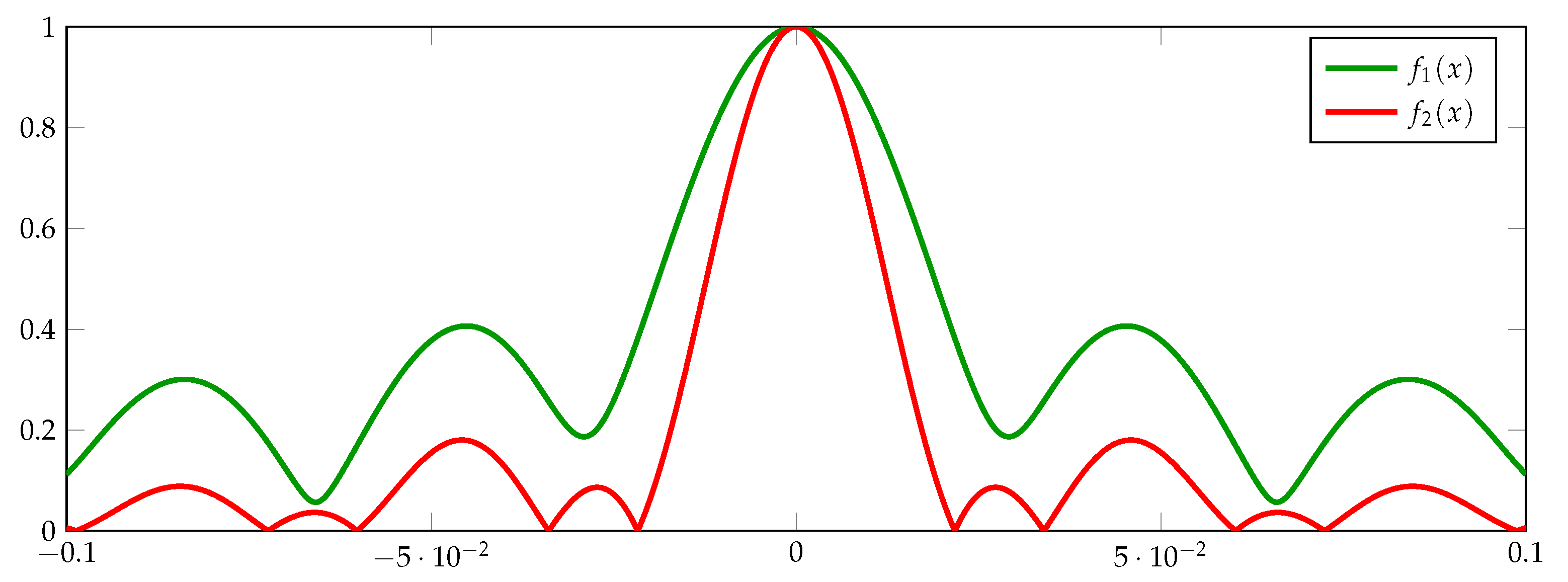
(Composition of Indicator Function). Similar to the indicator function with a single source, the factor $J_0\left(k\right|\mathbf{r}-{\mathbf{r}}^{\prime }{\left|\right)}^2$ contributes to the object detection while the remaining factors disturb the object detection and generate several artifacts. In contrast, the imaging performance of the ${\mathfrak{F}}_{MSM}(\mathbf{r},C)$ is independent of the transmitter’s location. To compare the imaging performance between single and multiple sources, we consider the following:

$$\begin{array}{cc}\hfill f_1\left(x\right)& =J_0\left(k\right|x\left|\right)+2{\displaystyle \sum _{p=1}^{{10}^5}}{i}^p{J}_p\left(k\right|x\left|\right)sinc\left({\displaystyle \frac{p\pi }{2}}\right)\hfill \\ \hfill f_2\left(x\right)& =J_0{\left(k\right|x\left|\right)}^2+2{\displaystyle \sum _{p=1}^{{10}^5}}{(-1)}^p{J}_p{\left(k\right|x\left|\right)}^{2}sinc\left({\displaystyle \frac{p\pi }{2}}\right).\hfill \end{array}$$

Note that these are similar to the 1D version of ${\mathfrak{F}}_{DSM}(\mathbf{r},m,0)$ and ${\mathfrak{F}}_{MSM}(\mathbf{r},0)$ with $\alpha =90°$ in the presence of a single object located at the origin. By comparing the plots in Figure 2, we can say that the application of multiple sources yields better images because less oscillation is involved than when imaging is performed with only a single source.

Figure 2. Plots of $f_1\left(x\right)$ and $f_2\left(x\right)$ at $f=4\mathrm{GHz}$.

Discussion 7

(Influence of Bistatic Angle). Based on (18), we observe that the imaging performance of ${\mathfrak{F}}_{MSM}(\mathbf{r},C)$ is highly dependent on $\alpha$. Similar to imaging with a single source, a good imaging result is expected when $\alpha$ is small; however, it is impossible to identify the objects when $\alpha$ is close to $\pi$.

Discussion 8

(Influence of Converted Constant). Here, we assume that $\mathbf{r}={\mathbf{r}}_s\in D_s$ for some s. Then, based on (18),

$$\begin{array}{c}\Lambda \left({\mathbf{r}}_s\right)+\Gamma ({\mathbf{r}}_s,C)\hfill \\ \hfill ={\displaystyle \frac{\#\left[\mathcal{I}\right(m\left)\right]}{8\sqrt{PQ}\pi }}{\int }_D\mathcal{O}\left({\mathbf{r}}^{\prime }\right)\mathrm{d}{\mathbf{r}}^{\prime }+{\displaystyle \frac{C\#\left[\mathcal{J}\right(m\left)\right]}{k}}\left(J_0\left(k\right|{\mathbf{r}}_s{\left|\right)}^2+2{\displaystyle \sum _{q=1}^{\infty }}{(-1)}^q{J}_q\left(k\right|{\mathbf{r}}_s{\left|\right)}^{2}sinc\left(q\alpha \right)\right).\end{array}$$

Thus, if C satisfies

$$\left|C\right|\ll \left|{\displaystyle \frac{karea\left(D_s\right)\#\left[\mathcal{I}\left(m\right)\right]}{8\pi \#\left[\mathcal{J}\left(m\right)\right]\sqrt{PQ}}}\left({\displaystyle \frac{{\epsilon }_s-{\epsilon }_0}{{\epsilon }_0{\mu }_0}}\right){\left(J_0\left(k\right|{\mathbf{r}}_s{\left|\right)}^2+2{\displaystyle \sum _{q=1}^{\infty }}{(-1)}^q{J}_q\left(k\right|{\mathbf{r}}_s{\left|\right)}^{2}sinc\left(q\alpha \right)\right)}^{-1}\right|,$$

then it is possible to recognize $D_s$ through the map of ${\mathfrak{F}}_{MSM}(\mathbf{r},C)$. Otherwise, if C satisfies the following inequality for all $s=1,2,\dots ,S$,

$$\left|C\right|\gg \left|{\displaystyle \frac{karea\left(D_s\right)\#\left[\mathcal{I}\left(m\right)\right]}{8\pi \#\left[\mathcal{J}\left(m\right)\right]\sqrt{PQ}}}\left({\displaystyle \frac{{\epsilon }_s-{\epsilon }_0}{{\epsilon }_0{\mu }_0}}\right){\left(J_0\left(k\right|{\mathbf{r}}_s{\left|\right)}^2+2\sum _{q=1}^{\infty }{(-q)}^1{J}_q\left(k\right|{\mathbf{r}}_s{\left|\right)}^{2}sinc\left(q\alpha \right)\right)}^{-1}\right|,$$

then it is very difficult to recognize the existence, location, and shape of the objects because the map of ${\mathfrak{F}}_{MSM}(\mathbf{r},C)$ only contains a peak of large magnitude at the origin.

Based on the above observations, similar to the imaging with a single source, the selection of C to identify $D_s$ is highly dependent on the ${\epsilon }_s$ values, the size of $D_s$, k, and the total number of transmitting and receiving antennas. Thus, $C=0$ is the best choice for a proper application of ${\mathfrak{F}}_{MSM}(\mathbf{r},C)$.

5. Results of Numerical Simulations

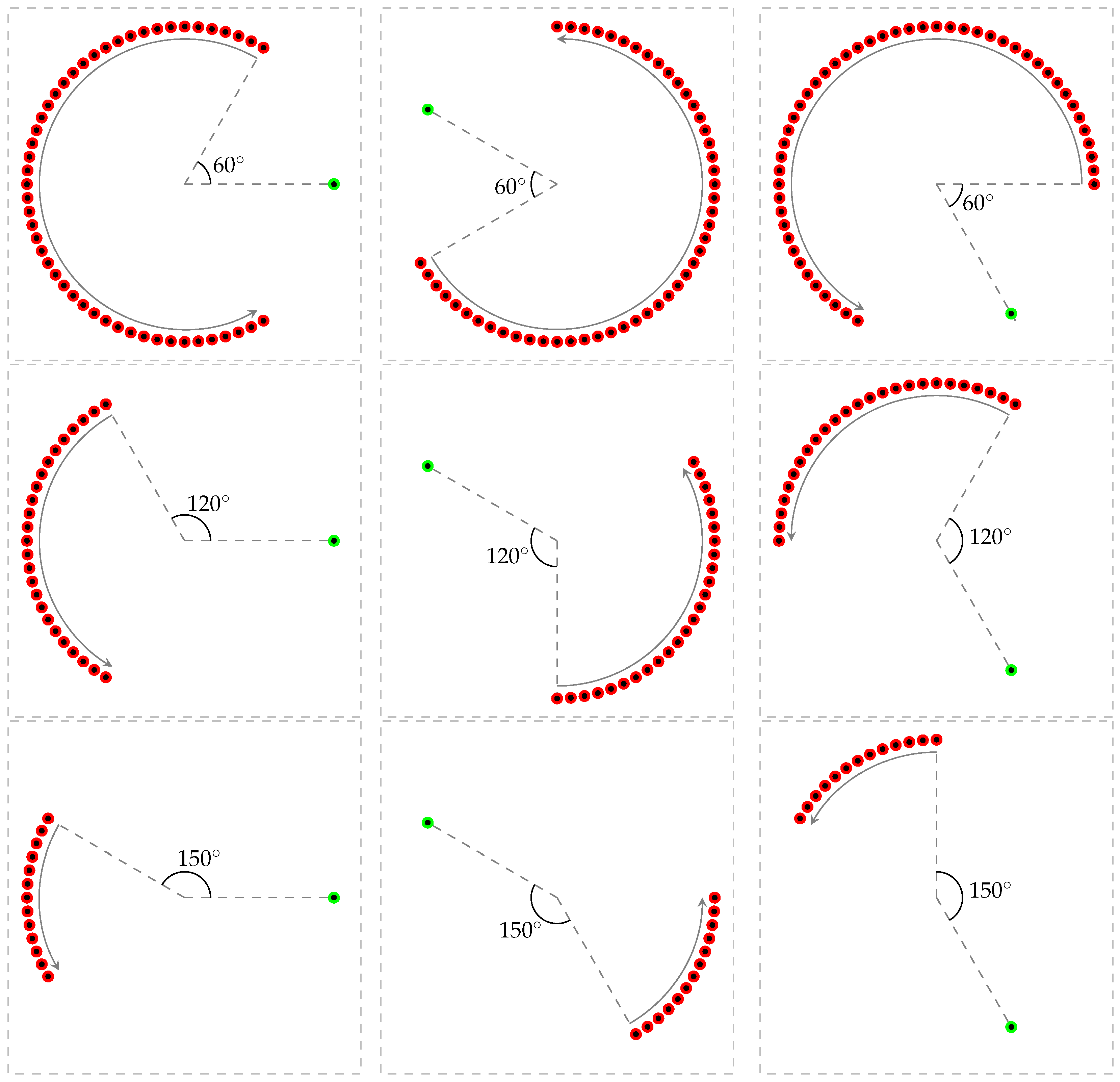
Here, the results of numerical simulations from the Fresnel dataset [39] with $f=4\mathrm{GHz}$ are presented to support the theoretical results and elucidate the discovered properties of the DSM. This dataset contains the scattered field data in the presence of two circular objects $D_s$, $s=1,2$ with centers ${\mathbf{r}}_1=(-0.045 \mathrm{m},0)$, ${\mathbf{r}}_2=(0.045 \mathrm{m},0.010 \mathrm{m})$, the same radii ${\alpha }_s=0.015 \mathrm{m}$, and the permittivity values ${\epsilon }_s=(3\pm 0.3){\epsilon }_0$. In addition, $M=36$ transmitters and $N=72$ receivers are positioned on circles centered at the origin with radii $\left|P\right|=0.72 \mathrm{m}$ and $\left|Q\right|=0.76 \mathrm{m}$, respectively. The range of receivers is restricted from $\alpha$ to $2\pi -\alpha$ with a step size of $▵\theta =5°$ based on each direction of the transmitters ${\vartheta }_m$, and the transmitters are distributed evenly with step sizes of $▵\vartheta =10°$ from $0°$ to $350°$. With this setting, the imaging results ${\mathfrak{F}}_{DSM}(\mathbf{r},m,C)$ with sources $m=1$, 16, and 31 (Figure 3 shows the antenna arrangements), and ${\mathfrak{F}}_{MSM}(\mathbf{r},C)$ with every source $m=1,2,\dots ,36$ were produced for each $\mathbf{r}\in \Omega$, where the imaging region $\Omega$ was selected as the square $[-0.1 \mathrm{m},0.1 \mathrm{m}]\times [-0.1 \mathrm{m},0.1 \mathrm{m}]$.

Figure 3. Antenna arrangements with various bistatic angles $\alpha =60°$, $120°$, and $150°$ corresponding to the transmitter ${\mathcal{P}}_1$ (left column), ${\mathcal{P}}_{16}$ (middle column), and ${\mathcal{P}}_{31}$ (right column). The green circle indicates the location of the transmitter, and the red circles show the arrangement of the receivers.

Example 1

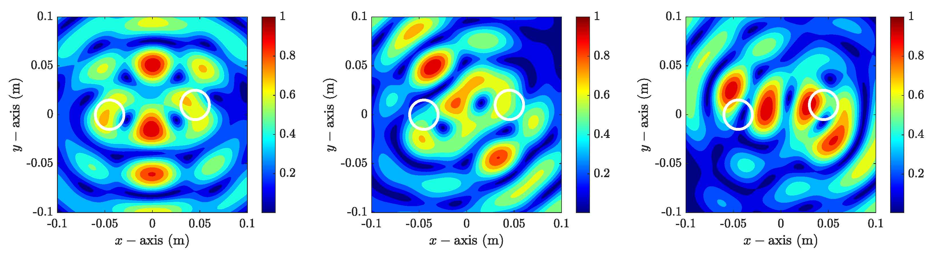
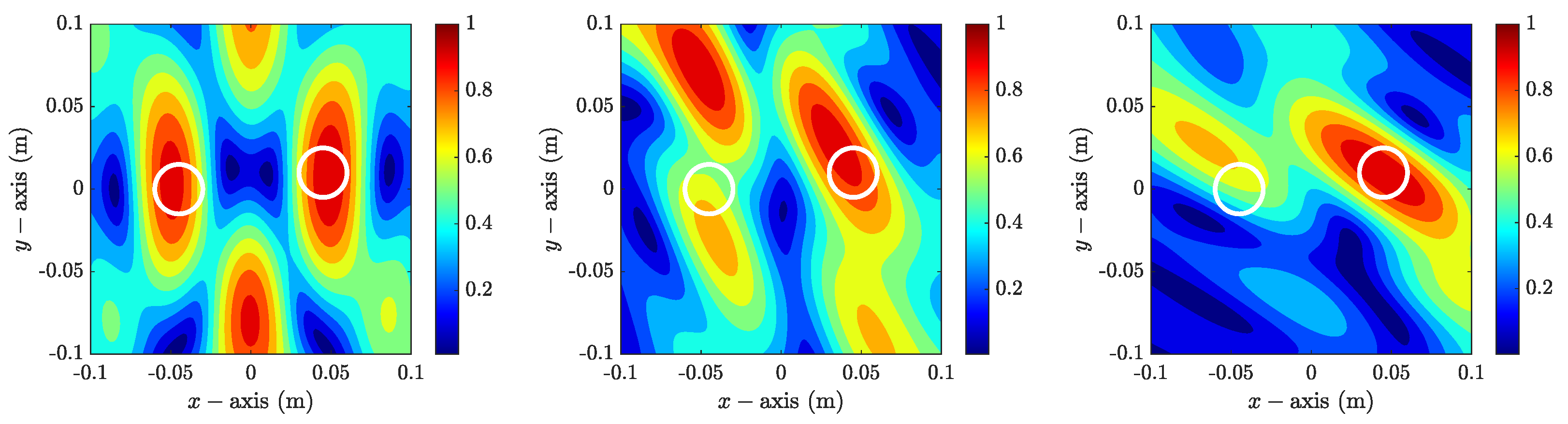
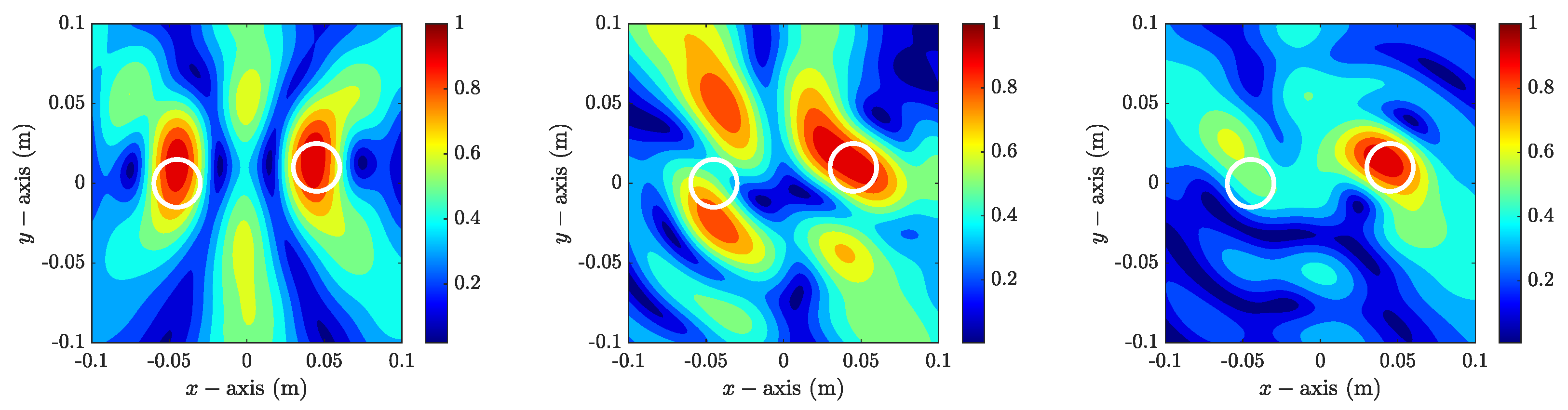
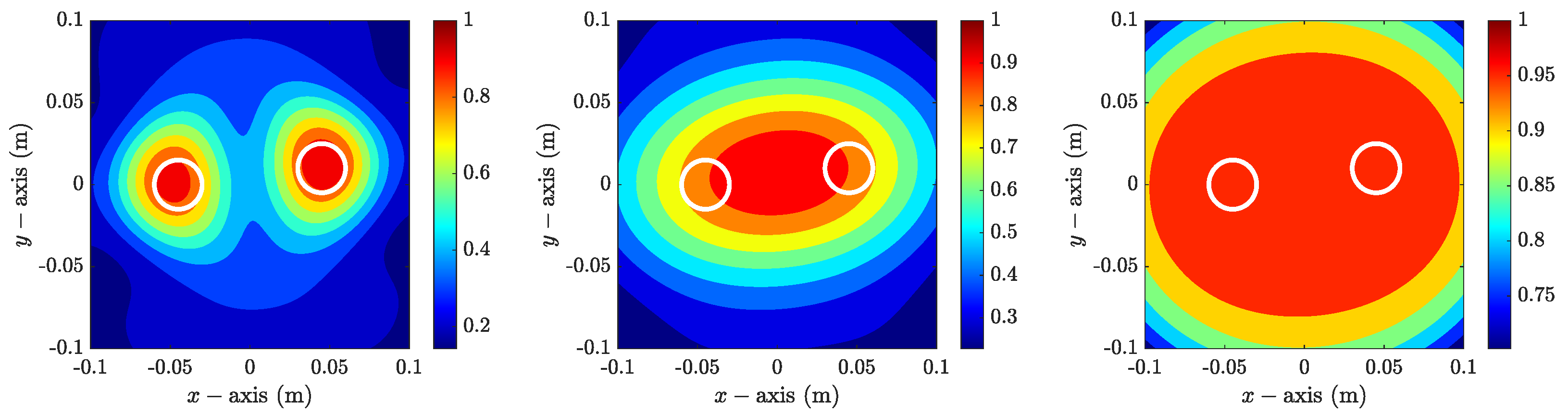
(Imaging With Zero Constant). Figure 4 shows maps of ${\mathfrak{F}}_{DSM}(\mathbf{r},m,0)$ with $\alpha =60°$ and various $m=1$, 16, and 31. Based on the results, it is possible to recognize the existence, nearly accurate location, and shape of $D_s$ when $m=1$. However, it is very difficult to recognize the existence of $D_1$ and $D_2$ due to the appearance of peaks of large magnitudes when $m=16$. Note that the existence of $D_2$ can be recognized; however, it is very difficult to recognize $D_1$ when $m=31$. Thus, the imaging performance of ${\mathfrak{F}}_{DSM}(\mathbf{r},m,0)$ is highly dependent on m, which supports Discussion 1.

Figure 4. (Example 1) Maps of ${\mathfrak{F}}_{DSM}(\mathbf{r},m,0)$ with $\alpha =60°$ for $m=1$ (left), $m=16$ (middle), and $m=31$ (right). The white circles describe the boundaries of the objects $D_1$ and $D_2$.

Example 2

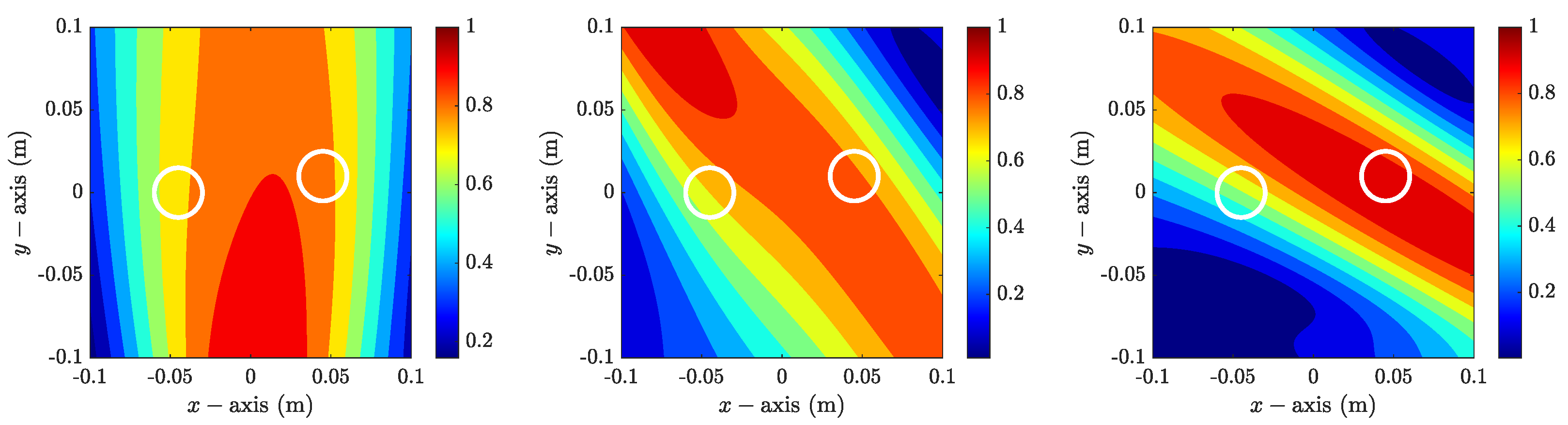
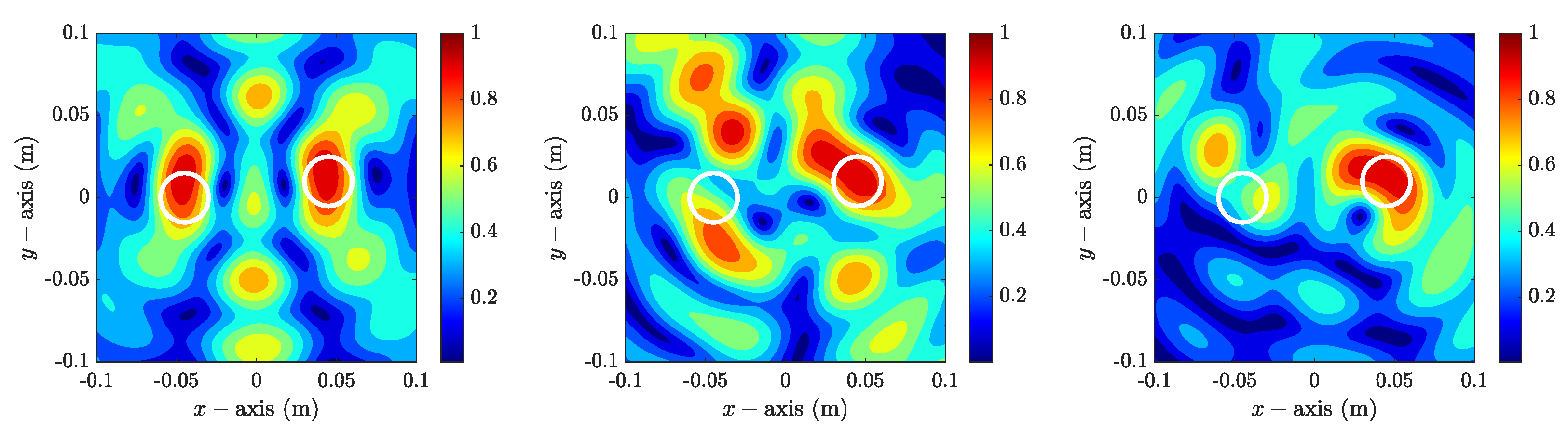
(Imaging With Nonzero Constant). Figure 5 shows maps of ${\mathfrak{F}}_{DSM}(\mathbf{r},m,0.1)$ with $\alpha =60°$ and various m. Similar to Example 1, here, the existence of $D_1$ and $D_2$ can be recognized; however, more artifacts are included when $m=1$. In addition, poor imaging results were obtained for $m=16$ and $m=31$.

Figure 5. (Example 2) Maps of ${\mathfrak{F}}_{DSM}(\mathbf{r},m,0.1)$ for $\alpha =60°$ with $m=1$ (left), $m=16$ (middle), and $m=31$ (right). The white circles describe the boundaries of the objects $D_1$ and $D_2$.

Figure 6 shows maps of ${\mathfrak{F}}_{DSM}(\mathbf{r},m,0.5i)$ with $\alpha =60°$ and various m. Compared with the results shown in Figure 5, in this case, it is impossible to recognize both $D_1$ and $D_2$ due to the appearance of several artifacts with large magnitudes. Based on the imaging results ${\mathfrak{F}}_{DSM}(\mathbf{r},m,2)$ obtained with $\alpha =60°$ and various m, it appears to be impossible to recognize $D_1$ and $D_2$ (Figure 7). Thus, based on Discussion 3, converting unmeasurable scattered field data into the zero constant (i.e., selecting $C=0$) is the best choice.

Figure 6. (Example 2) Maps of ${\mathfrak{F}}_{DSM}(\mathbf{r},m,0.5i)$ for $\alpha =60°$ with $m=1$ (left), $m=16$ (middle), and $m=31$ (right). The white circles describe the boundaries of the objects $D_1$ and $D_2$.

Figure 7. (Example 2) Maps of ${\mathfrak{F}}_{DSM}(\mathbf{r},m,2)$ for $\alpha =60°$ with $m=1$ (left), $m=16$ (middle), and $m=31$ (right). The white circles describe the boundaries of the objects $D_1$ and $D_2$.

Example 3

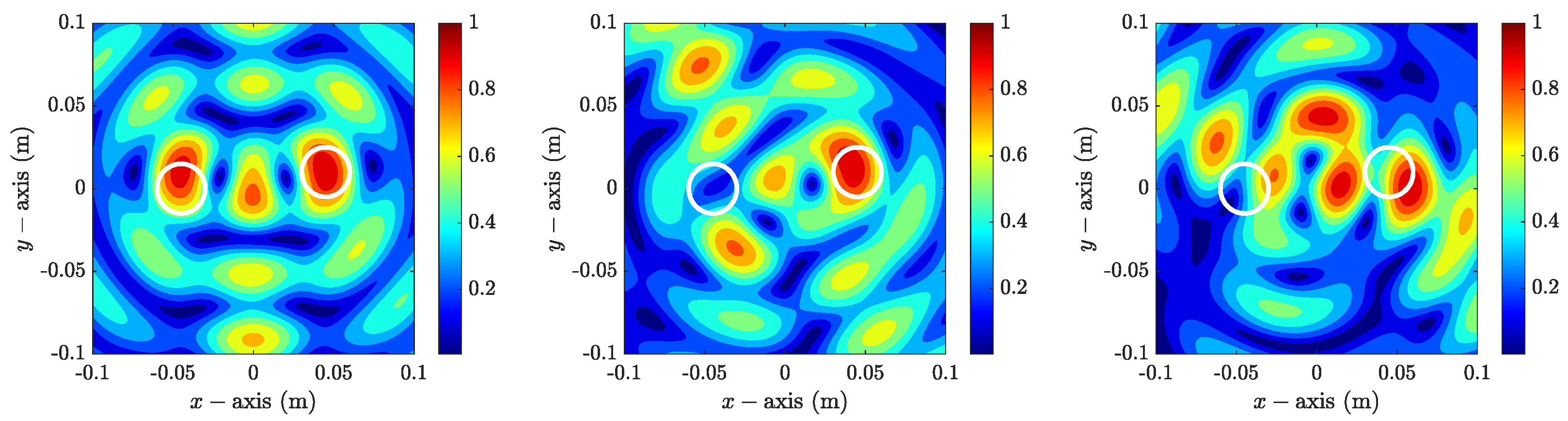
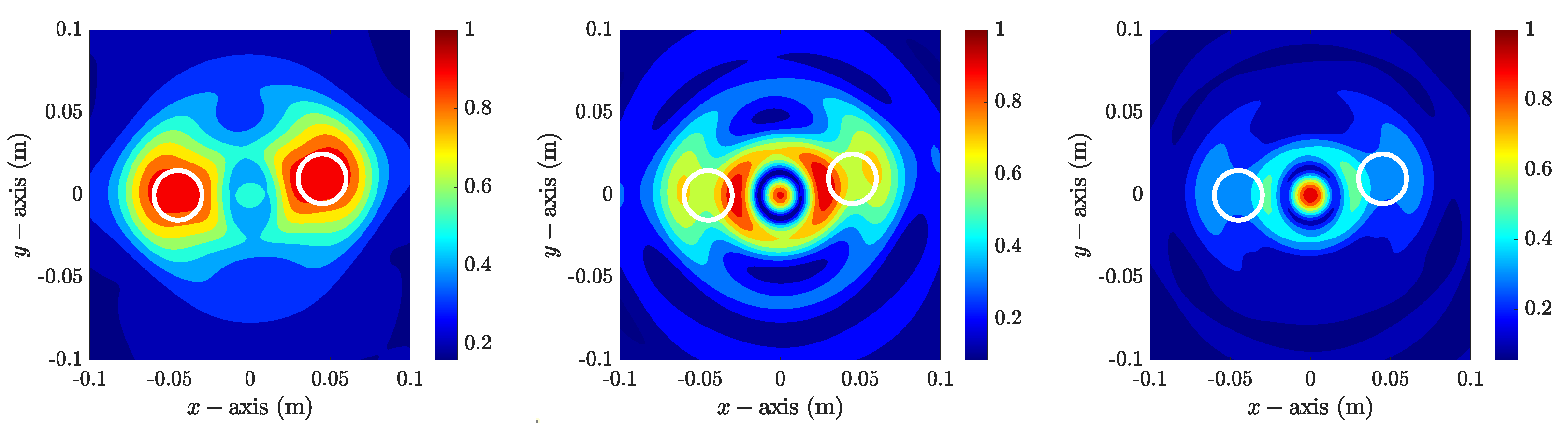
(Imaging With Various Bistatic Angles). Figure 8 shows maps of ${\mathfrak{F}}_{DSM}(\mathbf{r},m,0)$ with $\alpha =120°$ and various m. In contrast to the result obtained for Example 1, here, it is very difficult to identify the outline shape of the objects. In addition, if $C=0.2$ is selected, a peak of large magnitude appears at the origin; thus, it is very difficult to distinguish the objects and artifact when $m=1$ (Figure 9). Furthermore, it is impossible to recognize the objects when $m=16$ and 31.

Figure 8. (Example 3) Maps of ${\mathfrak{F}}_{DSM}(\mathbf{r},m,0)$ for $\alpha =120°$ with $m=1$ (left), $m=16$ (middle), and $m=31$ (right). The white circles describe the boundaries of objects $D_1$ and $D_2$.

Figure 9. (Example 3) Maps of ${\mathfrak{F}}_{DSM}(\mathbf{r},m,0.2)$ for $\alpha =120°$ with $m=1$ (left), $m=16$ (middle), and $m=31$ (right). The white circles describe the boundaries of objects $D_1$ and $D_2$.

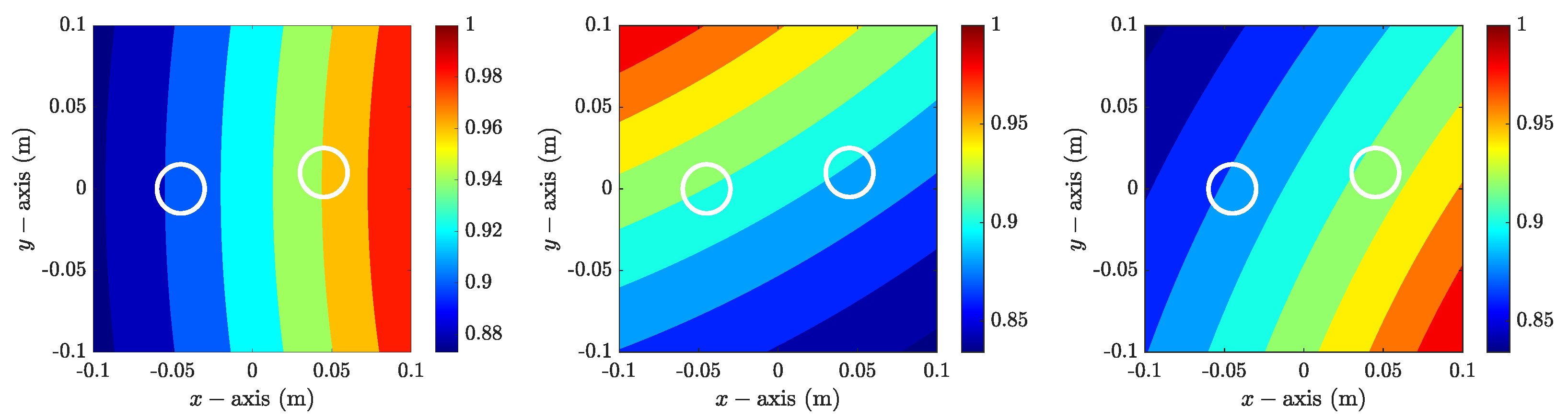
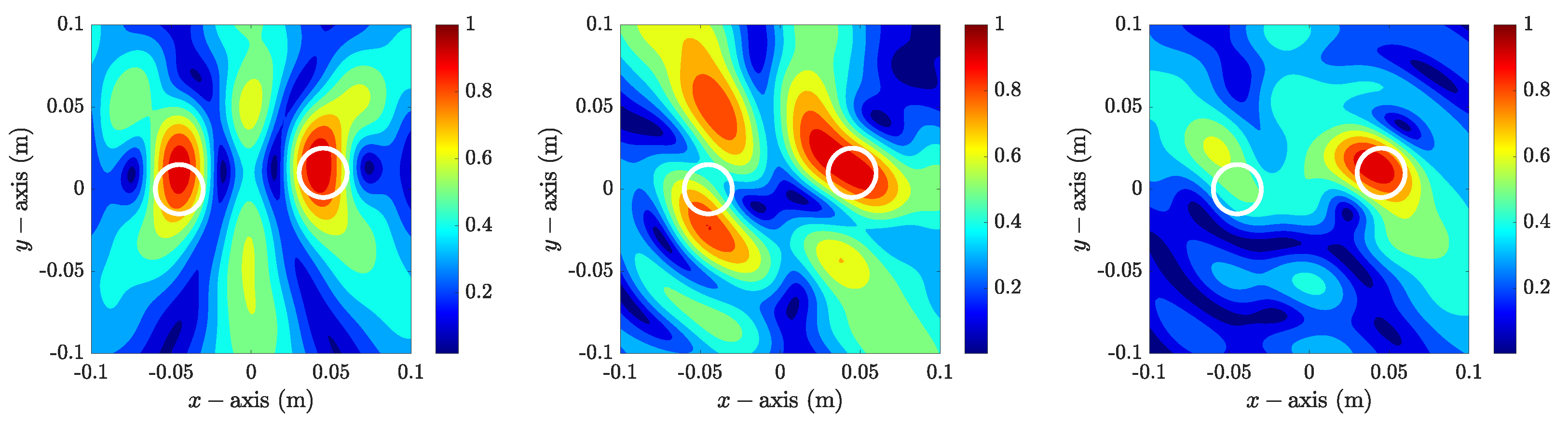
Figure 10 shows maps of ${\mathfrak{F}}_{DSM}(\mathbf{r},m,0)$ with $\alpha =150°$ and various m. In contrast to the previous results, it is impossible to recognize the existence of the objects because peaks of large magnitudes do not appear at the objects. In addition, if $\alpha =180°$, as observed in Discussion 2, nothing can be recognized because there is no peak of large magnitude as shown in Figure 11.

Figure 10. (Example 3) Maps of ${\mathfrak{F}}_{DSM}(\mathbf{r},m,0)$ for $\alpha =150°$ with $m=1$ (left), $m=16$ (middle), and $m=31$ (right). The white circles describe the boundaries of objects $D_1$ and $D_2$.

Figure 11. (Example 3) Maps of ${\mathfrak{F}}_{DSM}(\mathbf{r},m,0)$ for $\alpha =180°$ with $m=1$ (left), $m=16$ (middle), and $m=31$ (right). The white circles describe the boundaries of objects $D_1$ and $D_2$.

Example 4

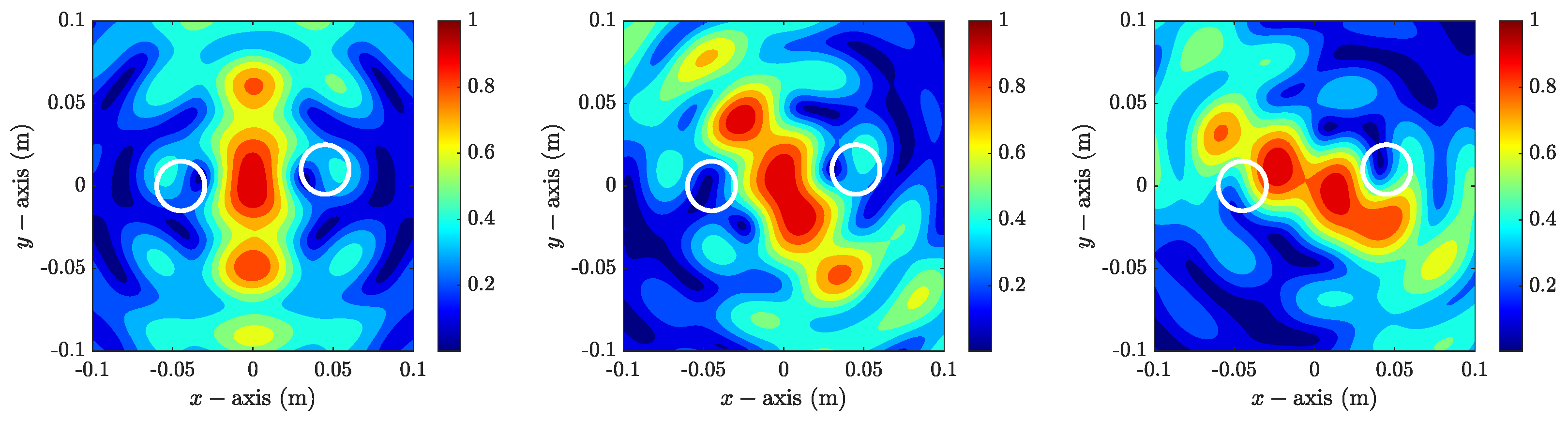
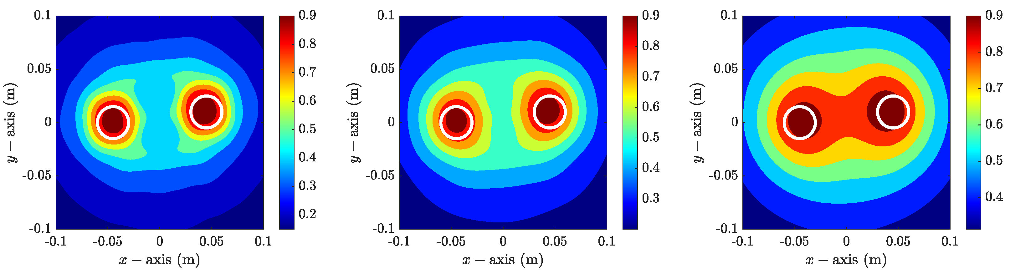
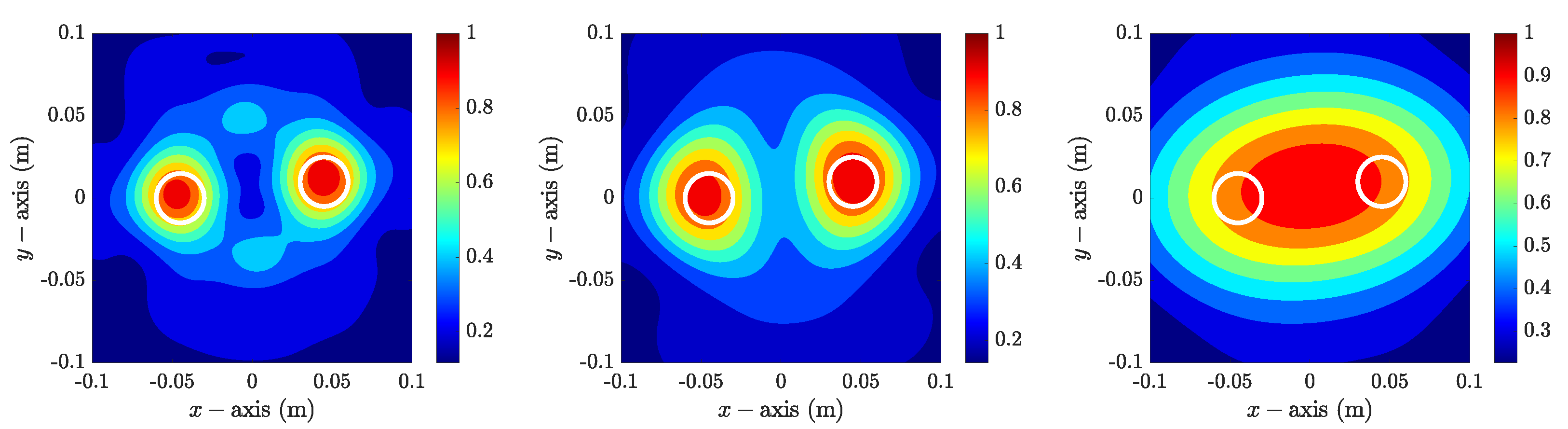
(Imaging With Multiple Sources). Figure 12 shows maps of ${\mathfrak{F}}_{MSM}(\mathbf{r},0)$ with various bistatic angle α values. Here, opposite to Example 3, it is possible to recognize the existence and approximate shape of both $D_1$ and $D_2$ for $\alpha =120°$. However, it remains impossible to retrieve the objects when $\alpha =150°$ and $180°$. Thus, we conclude that the DSM with multiple sources improves the imaging performance, but it is impossible to retrieve the objects when α approaches $180°$.

Figure 12. (Example 4) Maps of ${\mathfrak{F}}_{MSM}(\mathbf{r},0)$ for $\alpha =120°$ (left), $\alpha =150°$ (middle), and $\alpha =180°$ (right). The white circles describe the boundaries of objects $D_1$ and $D_2$.

Example 5

(Imaging With Multiple Sources with Nonzero Constant). Now, we consider the imaging results with various constant C with bistatic angle $\alpha =120°$. Based on Figure 13, it is possible to recognize the existence and location of the objects but their outline shapes cannot be identified when $C=0.1$. Notice that since the values of ${\mathfrak{F}}_{MSM}(\mathbf{r},0.3i)$ are significantly large at the origin and its neighborhood, it seems very difficult to recognize the presence of objects. When a larger C value ($C=0.5$) is applied, since the maximum value of ${\mathfrak{F}}_{MSM}(\mathbf{r},0.5)$ appears only at the origin, it is impossible to recognize the presence of the objects.

Figure 13. (Example 5) Maps of ${\mathfrak{F}}_{MSM}(\mathbf{r},C)$ for $\alpha =120°$ and $C=0.1$ (left), $C=0.3i$ (middle), and $C=0.5$ (right). The white circles describe the boundaries of objects $D_1$ and $D_2$.

Example 6

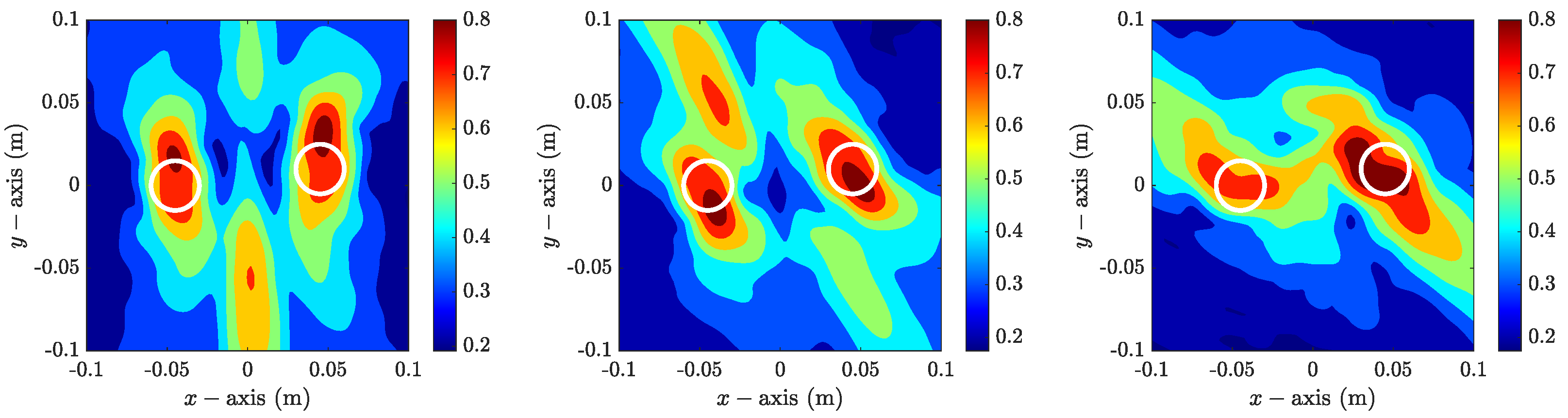
(Further Result: Robustness to Random Noise). Here, we consider the imaging results when the measurement data were corrupted by $20\mathrm{dB}$ white Gaussian noise. Figure 14 shows the maps of ${\mathfrak{F}}_{DSM}(\mathbf{r},m,0)$ for $m=1$, 16, and 31 with $\alpha =60°$. By comparing with Figure 4, we obtain similar results, indicating that the designed indicator function is robust to random noise. Figure 15 shows the maps of ${\mathfrak{F}}_{MSM}(\mathbf{r},0)$ with $\alpha =60°$, $\alpha =120°$, and $\alpha =150°$ in the presence of noice. Similar to the imaging with a single source, comparison with Figure 12 shows that the designed indicator function with multiple sources is robust to random noise.

Figure 14. (Example 6) Maps of ${\mathfrak{F}}_{DSM}(\mathbf{r},m,0)$ with noisy data for $\alpha =60°$: $m=1$ (left), $m=16$ (middle), and $m=31$ (right). The white circles describe the boundaries of the objects $D_1$ and $D_2$.

Figure 15. (Example 6) Maps of ${\mathfrak{F}}_{MSM}(\mathbf{r},0)$ with noisy data for $\alpha =60°$ (left), $\alpha =120°$ (middle), and $\alpha =150°$ (right). The white circles describe the boundaries of the objects $D_1$ and $D_2$.

Example 7

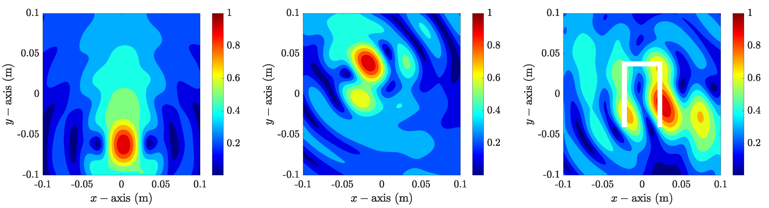
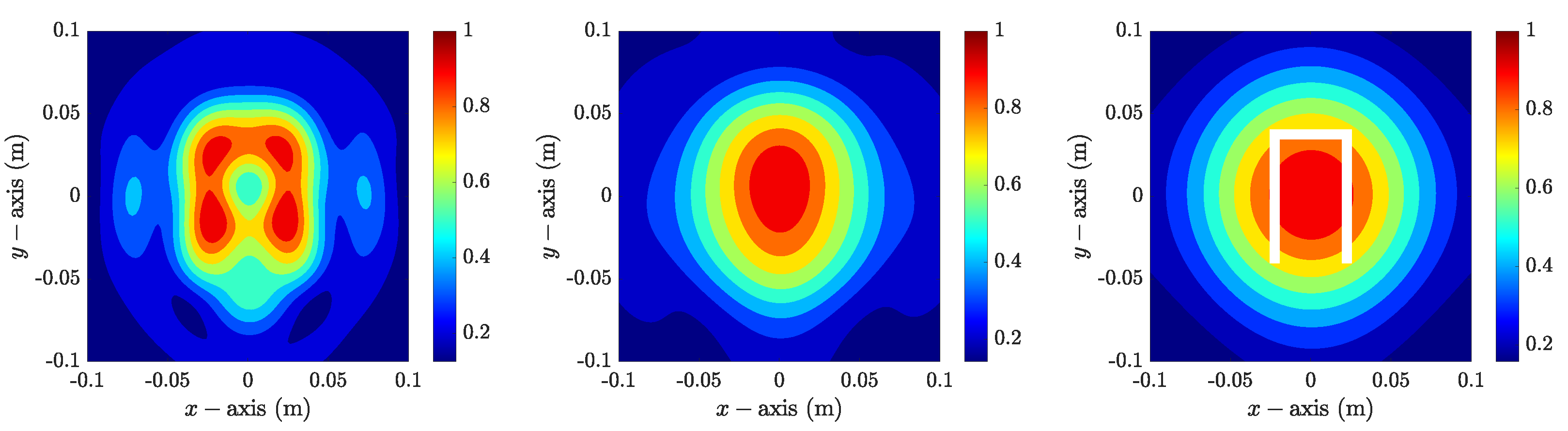
(Further Result: Imaging of Complex Shaped Object). Here, we consider the imaging of U-shaped metallic object (denoted by Γ) from the dataset uTM_shaped.exp; refer to [39]. As in Example 6, the measurement data were polluted by $20\mathrm{dB}$ white Gaussian noise. Figure 16 shows maps of ${\mathfrak{F}}_{DSM}(\mathbf{r},m,0)$ for $m=1,16,31$ with $\alpha =60°$. Unlike the imaging of small objects, it is impossible to recognize the shape of the metallic object. Therefore, it can be concluded that the designed indicator function with a single source is unsuitable for identifying complex-shaped objects. Fortunately, it is possible to recognize the outline of Γ througth the map of ${\mathfrak{F}}_{MSM}(\mathbf{r},0)$ with $\alpha =60°$ (see Figure 17). However, when the bistatic angle is wide, it is impossible to identify the shape of Γ , as shown in Figure 17 for $\alpha =120°$ and $\alpha =150°$. Hence, it can be concluded that the designed indicator function with multiple sources is suitable for identifying complex-shaped objects only when the range of the bistatic angle is not wide.

Figure 16. (Example 7) Maps of ${\mathfrak{F}}_{DSM}(\mathbf{r},m,0)$ with noisy data for $\alpha =60°$: $m=1$ (left), $m=16$ (middle), and $m=31$ (right). The white U-shaped line describes the true object.

Figure 17. (Example 7) Maps of ${\mathfrak{F}}_{MSM}(\mathbf{r},0)$ with noisy data for $\alpha =60°$ (left), $\alpha =120°$ (middle), and $\alpha =150°$ (right). The white U-shaped line describes the true object.

Example 8

(Further Result: Multi-Frequency Imaging). For the final example, we consider the imaging results using multiple frequencies with single and multiple sources. To this end, we introduce a set of frequencies $F=\left\{f:f=1,2,\dots ,8\mathrm{GHz}\right\}$ and the following imaging functions:

$${\mathfrak{F}}_{DSMM}(\mathbf{r},m,C)={\displaystyle \frac{1}{\#\left[F\right]}}\sum _{f\in F}{\mathfrak{F}}_{DSM}^{\left(f\right)}(\mathbf{r},m,C)\mathrm{and}{\mathfrak{F}}_{MSMM}(\mathbf{r},C)={\displaystyle \frac{1}{\#\left[F\right]}}\sum _{f\in F}{\mathfrak{F}}_{MSM}^{\left(f\right)}(\mathbf{r},C),$$

where ${\mathfrak{F}}_{DSM}^{\left(f\right)}(\mathbf{r},m,C)$ and ${\mathfrak{F}}_{MSM}^{\left(f\right)}(\mathbf{r},C)$ are the indicator functions defined in (8) and (17), respectively, at the given operating frequency f. Based on the imaging results with single-source in Figure 18, although it can be observed that the imaging performance has improved compared with the results in Figure 4, it is still difficult to conclude that good imaging results have been achieved. On the other hand, it is observed that the multiple-source imaging results in Figure 19 remain very good as long as the value of α is not excessively large. This is consistent with previous studies [46,47,48], confirming that the multi-frequency DSM successfully improves the imaging performance.

Figure 18. (Example 8) Maps of ${\mathfrak{F}}_{DSMM}(\mathbf{r},m,0)$ with noisy data for $\alpha =60°$: $m=1$ (left), $m=16$ (middle), and $m=31$ (right). The white circles describe the boundaries of objects $D_1$ and $D_2$.

Figure 19. (Example 8) Maps of ${\mathfrak{F}}_{MSMM}(\mathbf{r},0)$ with noisy data for $\alpha =60°$ (left), $\alpha =120°$ (middle), and $\alpha =150°$ (right). The white circles describe the boundaries of objects $D_1$ and $D_2$.

6. Concluding Remarks

In this paper, we considered the application of the DSM for rapid detection of small dielectric targets from a limited-aperture scattered-field data. To achieve this, we designed indicator functions for both single and multiple transmitters by replacing the unknown measurement data with a prescribed constant. To clarify the imaging performance of indicator functions and the roles of the chosen constant and bistatic angle, we showed that the indicator functions can be formulated as an infinite series of integer-order Bessel functions, material properties, specified constant, and bistatic angle. Theoretical results indicated that setting the conversion constant to zero and employing a small bistatic angle yields favorable results. The results of various numerical simulations conducted on a 2D Fresnel dataset were presented to support these theoretical results.

In this paper, we considered the identification of small objects embedded in a homogeneous domain using a two-dimensional Fresnel experimental dataset. The identification of unknown objects embedded in complex environments is an interesting subject for future research. Finally, an extension of the current study using three-dimensional Fresnel experimental dataset [49] is anticipated.

References

- Sasada, S.; Masumoto, N.; Song, H.; Emi, A.; Kadoya, T.; Arihiro, K.; Kikkawa, T.; Okada, M. Microwave breast imaging using rotational bistatic impulse radar for the detection of breast cancer: Protocol for a prospective diagnostic study. JMIR Res. Protoc. 2020, 9, e17524. [Google Scholar] [CrossRef] [Scilit] [PubMed]
- Persson, M.; Fhager, A.; Trefnà, H.D.; Yu, Y.; McKelvey, T.; Pegenius, G.; Karlsson, J.E.; Elam, M. Microwave-based stroke diagnosis making global prehospital thrombolytic treatment possible. IEEE Trans. Biomed. Eng. 2014, 61, 2806–2817. [Google Scholar] [CrossRef] [Scilit]
- Haynes, M.; Stang, J.; Moghaddam, M. Real-time microwave imaging of differential temperature for thermal therapy monitoring. IEEE Trans. Biomed. Eng. 2014, 61, 1787–1797. [Google Scholar] [CrossRef] [Scilit] [PubMed]
- Feng, M.Q.; Flaviis, F.D.; Kim, Y.J. Use of microwaves for damage detection of fiber reinforced polymer-wrapped concrete structures. J. Eng. Mech. 2002, 128, 172–183. [Google Scholar] [CrossRef] [Scilit]
- Henriksson, T.; Lambert, M.; Lesselier, D. Non-iterative MUSIC-type algorithm for eddy-current nondestructive evaluation of metal plates. In Electromagnetic Nondestructive Evaluation (XIV); Studies in Applied Electromagnetics and Mechanics; IOS Press: Amsterdam, The Netherlands, 2011; Volume 35, pp. 22–29. [Google Scholar]
- Foudazi, A.; Mirala, A.; Ghasr, M.T.; Donnell, K.M. Active microwave thermography for nondestructive evaluation of surface cracks in metal structures. IEEE Trans. Instrum. Meas. 2019, 68, 576–585. [Google Scholar] [CrossRef] [Scilit]
- Brovoll, S.; Berger, T.; Paichard, Y.; Aardal, Ø.; Lande, T.S.; Hamran, S. Time-lapse imaging of human heart motion with switched array UWB radar. IEEE Trans. Biomed. Circuits Syst. 2014, 8, 704–715. [Google Scholar] [CrossRef] [Scilit]
- Delbary, F.; Erhard, K.; Kress, R.; Potthast, R.; Schulz, J. Inverse electromagnetic scattering in a two-layered medium with an application to mine detection. Inverse Probl. 2008, 24, 015002. [Google Scholar] [CrossRef] [Scilit]
- Wu, S.; Zhou, H.; Liu, S.; Duan, R. Improved through-wall radar imaging using modified Green’s function-based multi-path exploitation method. EURASIP J. Adv. Signal Process. 2020, 2020, 4. [Google Scholar] [CrossRef] [Scilit]
- Ammari, H. Mathematical Modeling in Biomedical Imaging II: Optical, Ultrasound, and Opto-Acoustic Tomographies; Lecture Notes in Mathematics; Springer: Berlin, Germany, 2011; Volume 2035. [Google Scholar]
- Aster, R.C.; Borchers, B.; Thurber, C.H. Parameter Estimation and Inverse Problems, 2nd ed.; Elsevier: Amsterdam, The Netherlands, 2013. [Google Scholar]
- Ammari, H.; Kang, H. Reconstruction of Small Inhomogeneities from Boundary Measurements; Lecture Notes in Mathematics; Springer: Berlin, Germnay, 2004; Volume 1846. [Google Scholar]
- Bleistein, N.; Cohen, J.; Stockwell, J.S., Jr. Mathematics of Multidimensional Seismic Imaging, Migration, and Inversion; Interdisciplinary Applied Mathematics; Springer: New York, NY, USA, 2001; Volume 13. [Google Scholar]
- Chernyak, V.S. Fundamentals of Multisite Radar Systems: Multistatic Radars and Multiradar Systems; CRC Press; Routledge: Boca Raton, FL, USA, 1998. [Google Scholar]
- Colton, D.; Kress, R. Inverse Acoustic and Electromagnetic Scattering Problems; Mathematics and Applications Series; Springer: New York, NY, USA, 1998; Volume 93. [Google Scholar]
- Nikolova, N.K. Introduction to Microwave Imaging; Cambridge University Press: Cambridge, UK, 2017. [Google Scholar]
- Parker, R.L. Geophysical Inverse Theory; Princeton Series in Geophysics; Princeton University Press: Princeton, NJ, USA, 1994. [Google Scholar]
- Kress, R. Inverse scattering from an open arc. Math. Meth. Appl. Sci. 1995, 18, 267–293. [Google Scholar] [CrossRef] [Scilit]
- Ahmad, S.; Strauss, T.; Kupis, S.; Khan, T. Comparison of statistical inversion with iteratively regularized Gauss Newton method for image reconstruction in electrical impedance tomography. Appl. Math. Comput. 2019, 358, 436–448. [Google Scholar] [CrossRef] [Scilit]
- Ireland, D.; Bialkowski, K.; Abbosh, A. Microwave imaging for brain stroke detection using Born iterative method. IET Microw. Antennas Propag. 2013, 7, 909–915. [Google Scholar] [CrossRef] [Scilit]
- Li, J.; Li, Z.; Huang, R.; Han, F. Electromagnetic FWI of 2-D inhomogeneous objects straddling multiple planar layers by finite-element boundary integral and Levenberg–Marquardt methods. IEEE Trans. Geosci. Remote Sens. 2025, 63, 2001012. [Google Scholar] [CrossRef] [Scilit]
- Mallorqui, J.J.; Joachimowicz, N.; Broquetas, A.; Bolomey, J.C. Quantitative images of large biological bodies in microwave tomography by using numerical and real data. Electron. Lett. 1996, 32, 2138–2140. [Google Scholar] [CrossRef] [Scilit]
- Kwon, O.; Seo, J.K.; Yoon, J.R. A real-time algorithm for the location search of discontinuous conductivities with one measurement. Comm. Pur. Appl. Math. 2002, 55, 1–29. [Google Scholar] [CrossRef] [Scilit]
- Ito, K.; Jin, B.; Zou, J. A direct sampling method to an inverse medium scattering problem. Inverse Probl. 2012, 28, 025003. [Google Scholar] [CrossRef] [Scilit]
- Ito, K.; Jin, B.; Zou, J. A direct sampling method for inverse electromagnetic medium scattering. Inverse Probl. 2013, 29, 095018. [Google Scholar] [CrossRef] [Scilit]
- Kang, S.; Lambert, M.; Park, W.K. Direct sampling method for imaging small dielectric inhomogeneities: Analysis and improvement. Inverse Probl. 2018, 34, 095005. [Google Scholar] [CrossRef] [Scilit]
- Kang, S.; Lambert, M. Structure analysis of direct sampling method in 3D electromagnetic inverse problem: Near- and far-field configuration. Inverse Probl. 2021, 37, 075002. [Google Scholar] [CrossRef] [Scilit]
- Kang, S.; Lambert, M.; Ahn, C.Y.; Ha, T.; Park, W.K. Single- and multi-frequency direct sampling methods in limited-aperture inverse scattering problem. IEEE Access 2020, 8, 121637–121649. [Google Scholar] [CrossRef] [Scilit]
- Chow, Y.T.; Ito, K.; Zou, J. A direct sampling method for electrical impedance tomography. Inverse Probl. 2014, 30, 095003. [Google Scholar] [CrossRef] [Scilit]
- Chow, Y.T.; Ito, K.; Liu, K.; Zou, J. Direct sampling method for diffusive optical tomography. SIAM J. Sci. Comput. 2015, 37, A1658–A1684. [Google Scholar] [CrossRef] [Scilit]
- Kang, S.; Lambert, M.; Park, W.K. Analysis and improvement of direct sampling method in the mono-static configuration. IEEE Geosci. Remote Sens. Lett. 2019, 16, 1721–1725. [Google Scholar] [CrossRef] [Scilit]
- Li, J.; Zou, J. A direct sampling method for inverse scattering using far-field data. Inverse Probl. Imag. 2013, 7, 757–775. [Google Scholar] [CrossRef] [Scilit]
- Harris, I.; Kleefeld, A. Analysis of new direct sampling indicators for far-field measurements. Inverse Probl. 2019, 35, 054002. [Google Scholar] [CrossRef] [Scilit]
- Bousba, S.; Guo, Y.; Wang, X.; Li, L. Identifying multipolar acoustic sources by the direct sampling method. Appl. Anal. 2020, 99, 856–879. [Google Scholar] [CrossRef] [Scilit]
- Harris, I.; Nguyen, D.L.; Nguyen, T.P. Direct sampling methods for isotropic and anisotropic scatterers with point source measurements. Inverse Probl. Imag. 2022, 16, 1137–1162. [Google Scholar] [CrossRef] [Scilit]
- Ahn, C.Y.; Ha, T.; Park, W.K. Direct sampling method for identifying magnetic inhomogeneities in limited-aperture inverse scattering problem. Comput. Math. Appl. 2020, 80, 2811–2829. [Google Scholar] [CrossRef] [Scilit]
- Son, S.H.; Lee, K.J.; Park, W.K. Application and analysis of direct sampling method in real-world microwave imaging. Appl. Math. Lett. 2019, 96, 47–53. [Google Scholar] [CrossRef] [Scilit]
- Kim, J.Y.; Lee, K.J.; Kim, B.R.; Jeon, S.I.; Son, S.H. Numerical and experimental assessments of focused microwave thermotherapy system at 925MHz. ETRI J. 2019, 41, 850–862. [Google Scholar] [CrossRef] [Scilit]
- Belkebir, K.; Saillard, M. Special section: Testing inversion algorithms against experimental data. Inverse Probl. 2001, 17, 1565–1571. [Google Scholar] [CrossRef] [Scilit]
- Park, W.K. On the application of subspace migration from scattering matrix with constant-valued diagonal elements in microwave imaging. AIMS Math. 2024, 9, 21356–21382. [Google Scholar] [CrossRef] [Scilit]
- Park, W.K. Application of Kirchhoff migration from two-dimensional Fresnel dataset by converting unavailable data into a constant. Mathematics 2024, 12, 3253. [Google Scholar] [CrossRef] [Scilit]
- Son, S.H.; Simonov, N.; Kim, H.J.; Lee, J.M.; Jeon, S.I. Preclinical prototype development of a microwave tomography system for breast cancer detection. ETRI J. 2010, 32, 901–910. [Google Scholar] [CrossRef] [Scilit]
- Slaney, M.; Kak, A.C.; Larsen, L.E. Limitations of imaging with first-order diffraction tomography. IEEE Trans. Microw. Theory Techn. 1984, 32, 860–874. [Google Scholar]
- Ammari, H.; Bonnetier, E.; Capdeboscq, Y. Enhanced resolution in structured media. SIAM J. Appl. Math. 2009, 70, 1428–1452. [Google Scholar]
- Solimene, R.; Cuccaro, A.; Ruvio, G.; Tapia, D.F.; O’Halloran, M. Beamforming and holography image formation methods: An analytic study. Opt. Express 2016, 24, 9077–9093. [Google Scholar] [CrossRef] [Scilit]
- Funes, J.F.; Perales, J.M.; Rapún, M.L.; Vega, J.M. Defect detection from multi-frequency limited data via topological sensitivity. J. Math. Imaging Vis. 2016, 55, 19–35. [Google Scholar]
- Moscoso, M.; Novikov, A.; Papanicolaou, G.; Tsogka, C. Robust multifrequency imaging with MUSIC. Inverse Probl. 2018, 35, 015007. [Google Scholar] [CrossRef] [Scilit]
- Muñoz, S.; Rapún, M.L. Towards flaw detection in welding joints via multi-frequency topological derivative methods. Comput. Math. Appl. 2024, 161, 121–136. [Google Scholar] [CrossRef] [Scilit]
- Geffrin, J.M.; Sabouroux, P. Continuing with the Fresnel database: Experimental setup and improvements in 3D scattering measurements. Inverse Probl. 2009, 25, 024001. [Google Scholar] [CrossRef] [Scilit]
Disclaimer/Publisher’s Note: The statements, opinions and data contained in all publications are solely those of the individual author(s) and contributor(s) and not of MDPI and/or the editor(s). MDPI and/or the editor(s) disclaim responsibility for any injury to people or property resulting from any ideas, methods, instructions or products referred to in the content. |
© 2025 by the author. Licensee MDPI, Basel, Switzerland. This article is an open access article distributed under the terms and conditions of the Creative Commons Attribution (CC BY) license (https://creativecommons.org/licenses/by/4.0/).