Collaborative Optimization of Cloud–Edge–Terminal Distribution Networks Combined with Intelligent Integration Under the New Energy Situation

Abstract

The complex electricity consumption situation on the customer side and large-scale wind and solar power generation have gradually shifted the traditional “source-follow-load” model in the power system towards the “source-load interaction” model. At present, the voltage regulation methods require excessive computing resources to accurately predict the fluctuating load under the new energy structure. However, with the development of artificial intelligence and cloud computing, more methods for processing big data have emerged. This paper proposes a new method for electricity consumption analysis that combines traditional mathematical statistics with machine learning to overcome the limitations of non-intrusive load detection methods and develop a distributed optimization of cloud–edge–device distribution networks based on electricity consumption. Aiming at problems such as overfitting and the demand for accurate short-term renewable power generation prediction, it is proposed to use the long short-term memory method to process time series data, and an improved algorithm is developed in combination with error feedback correction. The R² value of the coupling algorithm reaches 0.991, while the values of RMSE, MAPE and MAE are 1347.2, 5.36 and 199.4, respectively. Power prediction cannot completely eliminate errors. It is necessary to combine the consistency algorithm to construct the regulation strategy. Under the regulation strategy, stability can be achieved after 25 iterations, and the optimal regulation is obtained. Finally, the cloud–edge–device distributed coevolution model of the power grid is obtained to achieve the economy of power grid voltage control.

1. Introduction

Since the Industrial Revolution, the large-scale utilization of fossil energy has brought great development to the social economy [1,2]. However, as time goes by, it has been found that fossil energy brings a series of negative impacts, such as the greenhouse effect [3,4,5]. Therefore, China has proposed the dual-carbon strategy [6,7], and the most important means to achieve it is the adjustment of the energy structure. The gradual replacement of fossil energy by clean energy is a new situation. Renewable energy is a typical clean energy, and the most important ones are solar and wind energy. However, it should be noted that wind and solar power generation have the characteristic of being “dependent on the weather”, so the power generation capacity is fluctuating and intermittent [8,9]. Under the new energy situation, higher requirements have been put forward for the regulation of distribution networks. Meanwhile, the traditional way of delivering power solely from plants to end customers through the power grid has been unable to adapt to complex electricity consumption situations [10]. Instead, the “source-load interaction” model is adopted. The electricity consumption at the customer end is also fed back into the power grid. This bidirectional flow mode can effectively improve the utilization of electricity and has the characteristic of being more flexible in adapting to renewable power generation. Facing the complex electricity consumption situations at the customer end and the integration of fluctuating renewable energy at the input end, how to respond promptly to various changes is the current research focus of the power grid.

In order to respond more quickly to complex changes in electrical energy, distributed control has emerged [11,12]. The control of the distribution network is stratified and graded, and each level regulates the distribution situation belonging to that level, which can achieve timely and flexible regulation and control. In addition, with the development of computer technology, a cloud–edge–device integrated technology combining artificial intelligence and edge computing has gradually emerged. By integrating edge resources, a large amount of data information can be processed, stored, and transmitted, but not all of the information will be sent to the cloud. This mitigates computational burdens [13,14,15]. The distributed collaboration of the cloud–edge–device distribution network structure is a control method proposed under the new energy situation. In view of the diverse electricity consumption at the customer end and the reality of renewable energy being connected to the grid, developing real-time distributed optimization of the distribution network, based on the accurate prediction of electricity consumption, and renewable power generation, to provide a more precise control basis for the distribution network regulation, are the current key points of research on new distribution networks.

The customer end mainly considers the random behavior of customers [16]. In the long term, electricity consumption has a certain regularity. For example, working during the day is the peak electricity consumption period, and resting at night is the low electricity consumption period. However, there are special circumstances where significant fluctuations may occur within a very short period of time. Therefore, short-term predictions are usually more difficult to make accurately than long-term ones [17]. In order to conduct effective energy management, a non-intrusive load monitoring method is used to manage the load of each device. Non-invasive monitoring based on families has shown good results [18]. After analysis, it is found that industrial production and commercial activities account for a large proportion of electricity consumption. These activities have relatively clear divisions of working and off-duty hours, which can provide the necessary conditions for high-level prediction. Welikala et al. [19] used non-intrusive methods to consider electrical appliances in industry and commerce, achieving accurate assessment and prediction of loads. Wurm et al. [20] adopted a non-invasive method to collect electrical loads and processed the data using clustering methods, demonstrating excellent prediction results. However, non-invasive methods with high precision and the ability to handle different devices quickly require a large amount of historical data and a complex training process to be realized [17]. Meanwhile, regarding the electricity consumption prediction at the customer end, the existing methods also have many problems that need to be urgently addressed. They have shown good effects for long-term stable power prediction. However, for the short term, especially in the case of extremely large power fluctuations, the current deep-learning methods cannot fit these data well [21,22]. Accurate prediction for similar situations is of great significance for the regulation and control of distributed distribution networks.

For the prediction methods of wind and solar power generation, there are usually statistical mathematics methods and artificial intelligence methods. Fan et al. [23] used traditional statistical mathematics methods to predict the renewable power generation and obtained relatively reasonable results. However, as the installed capacity of renewable energy increases, the sample database becomes increasingly large, making it difficult to handle. Artificial intelligence is a better way to handle big data [13,14]. Artificial neural networks are a type of artificial intelligence algorithm, which have good nonlinear fitting and self-learning feedback capabilities. However, excessive fitting of neural networks is prone to cause a decrease in accuracy. Wang et al. [24] conducted coupling optimization using random forests and artificial neural network models. The coupled model could obtain accurate predicted values, but it is computationally complex. Deep neural networks represent one of the various architectural developments in artificial neural networks. They have more hidden layers and can achieve better results in complex events. Fan et al. [25] used the deep neural network algorithm for the prediction of renewable power generation and simultaneously adopted the restricted Boltzmann machine and the modified linear correlation for coefficient regulation. The accuracy was significantly improved, but the phenomenon of overfitting still occurred.

For customer-side electricity consumption prediction, customer demands and customer behaviors are directly related. Due to demand, customers take actions, and these actions generate electricity consumption. Non-intrusive methods and particle swarm optimization algorithms are combined to construct a hybrid algorithm. The influence of equipment startup and shutdown is considered in the algorithm, effectively improving the prediction accuracy. For the power generation side, an improved long short-term memory method is obtained in combination with error feedback correction. The wind and solar power generation have been accurately predicted. A complete closed loop for power prediction on both the customer side and the power generation side has been formed. However, power prediction has a certain degree of error. At the same time, a consistency optimization strategy is proposed for real-time regulation and control. Ultimately, the intelligent control strategy for cloud–edge–terminal distribution networks under the new energy situation is obtained.

2. Construction of a Distributed Optimization Model for Cloud-Edge-Device Distribution Networks Based on Customer-Side Demands

First, the general process of model construction is introduced. This study is based on the multi-level resource scheduling technology of cloud–edge–device to construct a distributed collaborative framework for the distribution network. The specific distributed collaborative framework of the cloud–edge–device distribution network is shown in Figure 1. The cloud–edge–end system is applied in power grid control, so the energy used is electrical energy. This study does not discuss the actual operation of the power generation side, whether it is coal-fired power generation or renewable power generation. It only considers the regulation and control of electricity in the power grid. The cloud side includes the control center and the power grid company, which are responsible for unified control [26,27,28]. The edge side includes multiple edge side servers, which can be used to control networks at all levels. The end side includes various electricity customers and power generation plants, which consume and generate electricity. Cloud–edge–device distributed collaboration optimally divides the control process hierarchically and decomposes the overall goal, efficiently allocating computing resources to address computational constraints during scaling.

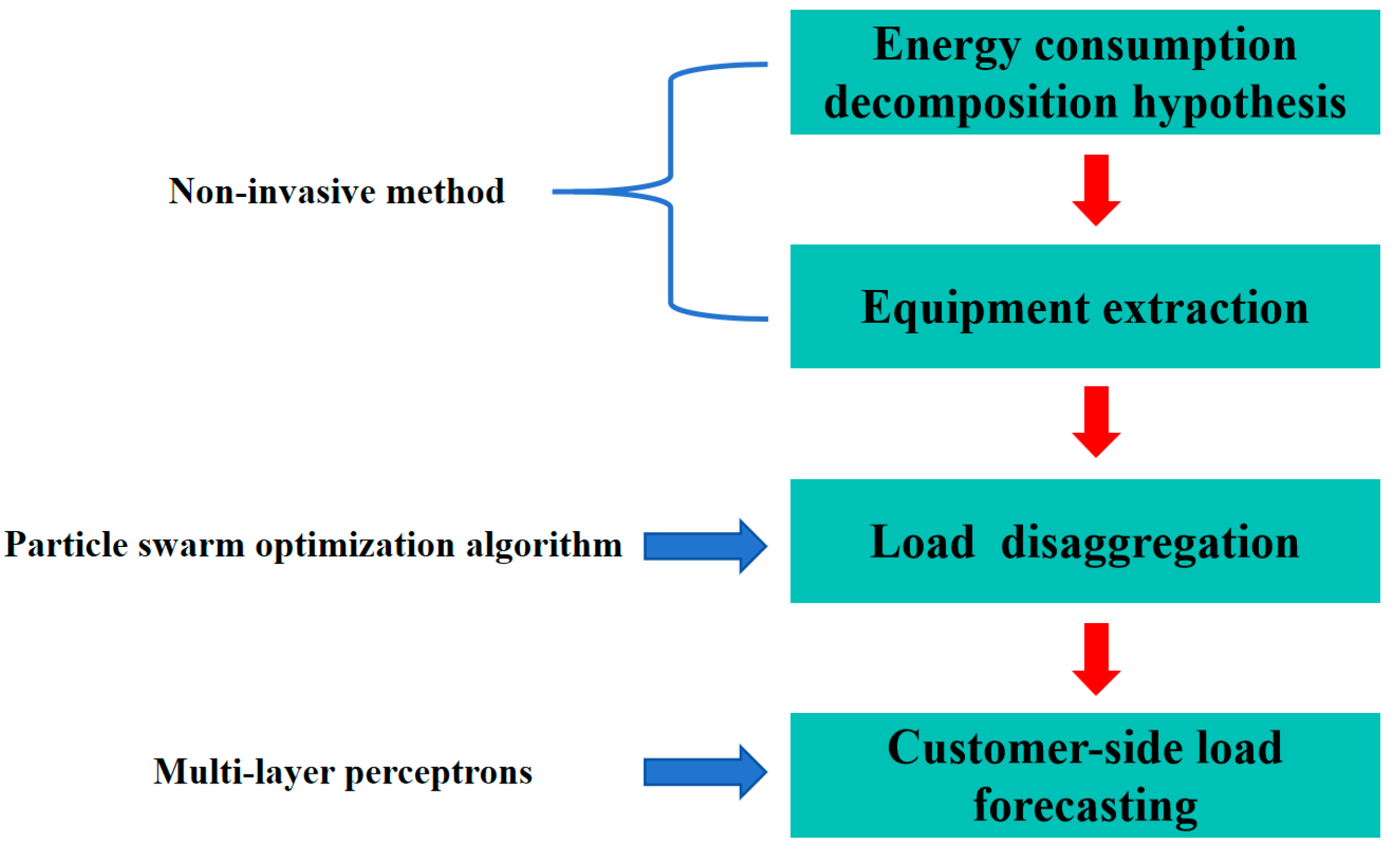
The following introduces the construction process of the customer-side electricity consumption prediction algorithm. First, the electricity consumption decomposition assumption is described. Then, the particle swarm is used to optimize the decomposition assumption to obtain the extraction process of the equipment. Finally, the prediction algorithm is obtained. The structure of the customer-side electricity consumption prediction algorithm can be shown in Figure 2.

A certain district in a certain city of China was selected as the research object. In this district, there are commercial, industrial, and residential areas. This area consists of six residential areas, two shopping malls, and one factory that produces machine tools. There are 2358, 3021, 3487, 1542, 3862, and 3379 households in the six residential areas, respectively. There are 56 and 35 shops in the two shopping malls, respectively. The factory is a small processing plant with 142 employees. At the same time, in order to obtain high-quality data, non-representative customers in the database were deleted, namely, customers with high electricity consumption at night and customers with low electricity consumption throughout the day. The final dataset consisted of 14,675 residential customers, 78 commercial customers, and 126 industrial customers. The data selection period was from December 2019 to December 2020, and the data was provided by the local power supply company. The dataset was divided, with 85% of the data used as the training set to regulate the coefficients. And 15% of the data was used as the testing set to test whether the proposed algorithm was overfitting. The data involved in the paper fully conform to the characteristics of big data [29]. They have the characteristics of large quantity, rapid growth, diverse data types, and the need for processing before obtaining the required effective information.

In the model debugged by the training set, the test set data is input to obtain the output data information. Accuracy rate (A), recall rate (R), and mean absolute percentage error (MAPE) are introduced to determine whether the model performance is qualified. The calculation formulas for P, R, and MAPE are shown in (1)–(3):

$$\mathrm{A}={\displaystyle \frac{N_{TP}}{N_{TP}+N_{FP}}}$$

(1)

$$R={\displaystyle \frac{N_{TP}}{N_{TP}+N_{FN}}}$$

(2)

$$\mathrm{MAPE}={\displaystyle \frac{1}{N}}\left[{\displaystyle \sum }_i^N{\displaystyle \frac{\left|Y_i-Y_i^{\prime }\right|}{Y_i}}\right]\times 100\%$$

(3)

In the formula, NTP represents the number of true class samples, NFP represents the number of false-positive class samples, and NFN represents the number of false-negative class samples. N represents the amount of data, and Y and Y’, respectively, represent the predicted value and the actual value.

2.1. Extraction Process of the Equipment

The equipment power is a sequence function of time [19,20]. Therefore, assuming that the equipment state is a combination of linear relationships over time, the equipment power can be shown by Formula (4):

$$P\left(t\right)={\displaystyle \sum }_{\begin{array}{c}i,t\\ s_i\left(t\right)=1\end{array}}{s}_i\left(t\right)l_i\left(t+\tilde{t}\right)P_i+{\displaystyle \sum }_{\begin{array}{c}i,t\\ s_i\left(t\right)=-1\end{array}}{s}_i\left(t\right)l_i\left(t\right)P_i+\epsilon \left(t\right)$$

(4)

In the formula, P(t) is the total power of the equipment at time t, t is time, $\tilde{t}$ is the time required for the device to reach the state, s is device status, i is device configuration information, l is device dynamic configuration information, Pi is the power of class i equipment, and ε is the error value Device configuration information i ∈ {0, 1, …, M}, and device status s ∈ state matrix {0, 1, −1}^TxM. s_i(t) is the t-th row and i-th column of s. When s_i(t) = 1, device i is switched on at time t. And for s_i(t) = −1, device i is switched off. When s_i(t) = 0, the state of device i remains the same.

$\tilde{t}$represents the time interval. Each device needs a certain amount of time to start up, of course. This specific time is determined by the type of device. This is the original power formula. In the subsequent part of the article, the power calculation formula is simplified, assuming that the equipment can be started or stopped instantaneously.

When calculating the power at time t, the first term includes the device’s startup. $l_i\left(t+\tilde{t}\right)$ represents the i device profile, including dynamic behavior and stable state. Specifically, the first term represents the power when i device starts at time t and begins to operate stably after $\tilde{t}$.

For residential, commercial, and industrial customers, the main focus is on the condition of the electrical equipment. In the electricity consumption, the relationship between active power and reactive power is unique and exclusive to the corresponding equipment.

As for the assumption of energy consumption decomposition, corresponding optimizations must be carried out to achieve an accurate description of power. The optimization process can be shown by Formula (5):

$$Min E\left(P, P_S\right)$$

(5)

In the formula, P represents the total power of the measured equipment, and P_s is the approximate power of the equipment calculated through Formula (4). In order to minimize the error values of calculation and measurement, it is necessary to clarify the functional relationship and the profile of the equipment.

The main electricity consumption are the equipments in daily life, industrial production and commercial activities [30]. Assuming that equipment is a binary state, there are only two states: on and off. The Gaussian mixture model is adopted to extract the effective information of the aggregated data signal to determine the equipment start/stop times [31,32]. In order to identify the sudden and significant decrease or increase in power within a short period of time, the study expresses it through the derivative of power, and its calculation can be shown by Formula (6):

$$\Delta P\left(t\right)={\displaystyle \frac{P\left(t+\Delta t\right)-P\left(t\right)}{\Delta t}}$$

(6)

In the formula, ΔP(t) is the derivative of power at time t, and Δt is the change in time.

All devices are assumed to be able to be turned on and off instantaneously. The peak standard is introduced to determine the event time of device activation, which can be determined by Formula (7):

$$t=t_p\to \Delta P_{tot}\left(t-1\right)<\Delta P_{tot}\left(t\right)\forall \Delta P_{tot}\left(t+1\right)<\Delta P_{tot}\left(t\right)$$

(7)

In the formula, P_tot is the sum of three-phase active power.

The increase or decrease in the three-phase positions of active power and reactive power can correspond to the characteristics of the corresponding equipment. According to this characteristic, this paper classifies the equipment and uniformly divides them into six categories and adopts the classic k-means clustering algorithm to process the sample database. For the specific mode of the device being turned on, the device being turned off is the exact opposite mode. Therefore, it is only necessary to conduct a cluster analysis on the on state. The sample database is divided. The set where the Euclidean distance of the data is the smallest to the cluster center belongs to the K-cluster. Meanwhile, the number of clusters is counted. The analysis method is shown by Formula (8):

$$min{\displaystyle \sum }_{n=1}^N{\displaystyle \sum }_{k=1}^K{r}_{nk}{\left|\Delta P\left(t_{p,n}\right)-\overrightarrow{c_k}\right|}^2$$

(8)

When the value of r_nk is one, the event ∆P(t_p,n) dataset belongs to the k cluster. When the value of rnk is zero, the event ∆P(t_p,n) dataset belongs to other clusters.

The k-means clustering algorithm maximizes the expected value to solve the problem of minimizing the Euclidean distance to the cluster center. To obtain the optimal value for a specific event, the Calinski–Harabasz index (CHI) is proposed, and its calculation formula is shown in Formula (9):

$$CHI={\displaystyle \frac{N-K}{K-1}}{\displaystyle \frac{{{\displaystyle \sum }}_{c_k\in C}\left|c_k\right|{\left|\overrightarrow{c_k}-\overrightarrow{D}\right|}^2}{{{\displaystyle \sum }}_{\overrightarrow{c_k}}{{\displaystyle \sum }}_{\Delta P\left(t_{p,i}\right)\in c_k}{\left|\Delta P\left(t_{p,i}\right)-\overrightarrow{c_k}\right|}^2}}$$

(9)

In the formula, N is the number of specific events, and D is the clustering center of the events. When CHI reaches its maximum value, the Euclidean distance of the event is the smallest.

In order to further simplify the data, clusters are merged based on a similarity measure. Whether two different clusters can be merged is determined by the Pearson correlation coefficient and the absolute percentage error. The Pearson correlation coefficient can be calculated by Formula (10):

$$\rho \left({\overrightarrow{c}}_i,{\overrightarrow{c}}_j\right)={\displaystyle \frac{{\sigma }_{{\overrightarrow{c}}_i,{\overrightarrow{c}}_j}}{{\sigma }_{{\overrightarrow{c}}_i}{\sigma }_{{\overrightarrow{c}}_j}}}$$

(10)

In the formula, ${\sigma }_{{\overrightarrow{c}}_i,{\overrightarrow{c}}_j}$ is the covariance of the different clusters. The absolute percentage error is calculated by Formula (11):

$$APE\left({\overrightarrow{c}}_i,{\overrightarrow{c}}_j\right)={\displaystyle \frac{\left|{\overrightarrow{c}}_i-{\overrightarrow{c}}_j\right|}{\left|{\overrightarrow{c}}_i\right|}}$$

(11)

When $\rho \left({\overrightarrow{c}}_i,{\overrightarrow{c}}_j\right)$ is greater than 0.9 and $APE\left({\overrightarrow{c}}_i,{\overrightarrow{c}}_j\right)$ is less than 0.1, the two clusters can be merged. A Gaussian mixture model is used to divide the running time. The probability calculation of the Gaussian mixture model is shown as Formula (12):

$$p\left(\theta |B\right)={\displaystyle \sum }_{i=1}^m{\pi }_{i}N(\left.\overrightarrow{x}\right|\overrightarrow{{\mu }_i},{{\displaystyle \sum }}_i)$$

(12)

In the formula, p(θ│B) is the parameter probability, and the average value in the Gaussian distribution can represent the running time. To obtain the running time from Formula (12), it is necessary to know the number m in the sub-distribution. In this study, the Bayesian information criterion is used to obtain the optimal quantity [33,34,35], which can be calculated by Formula (13):

$$BIC={\displaystyle \frac{1}{2}}MlnN-lnp\left(B|\theta \right)$$

(13)

In the formula, N represents the number of samples in the dataset, and B and M are the state parameters of θ.

2.2. Particle Swarm Optimization Algorithm for Decomposition Optimization

In this paper, the particle swarm optimization algorithm is adopted to optimize and decompose the clusters, with the aim of extracting the hidden information in each combination [36]. The equipment status is classified as “on” (1), “off” (−1), and “Maintain status” (0). Power at time t can be described as the superposition of individual device types 1-M, and, thus, can form a state matrix {0, 1, −1}^TxM. The particle swarm optimization algorithm determines the state change of each matrix data set and minimizes the error value. Its decomposition process can be shown by Formula (14):

$$E^{\left(a,b\right)}\left(P,P_S\right)=a{\displaystyle \sum }_{t=a}^{b-1}{\left({\overrightarrow{P}}_S\left(t\right)-\overrightarrow{P}\left(t\right)\right)}^2+\beta {\displaystyle \sum }_{t=a}^{b-2}{\left(\Delta {\overrightarrow{P}}_S\left(t\right)-\Delta \overrightarrow{P}\left(t\right)\right)}^2$$

(14)

In the formula, α + β = 1. The status of the equipment is divided into a transient switch state or a stable state, and the load curve of the equipment represents the behavior of the equipment.

When initializing the particle swarm optimization algorithm, the position matrix is set to 0, and events are randomly added to 3% of the entries. The total signal passing through is divided by time, and initialization is required in each period. The selection of hyperparameters depends on the optimization problem itself and the convergence speed. However, due to the limited computing resources, the selection of hyperparameters cannot be infinite. For decomposition, the maximum number of periods is 50, and each period can be iterated up to 30 times at most. The particle swarm optimization algorithm is initialized to 10 particles.

2.3. Power Prediction Algorithm for Customer-Side Electricity Consumption

Welikala et al. [19] used non-intrusive methods to predict power and showed good results but also found that computing resources were an important factor affecting the prediction accuracy. Subsequently, Wurm et al. [20] conducted a cluster analysis on the devices in the preprocessing, which could effectively screen the data. However, for the situation of power mutation, there is currently a lack of consideration. Even the advanced neural network structures at present have difficulty fitting these data well [22]. This study proposes a new method based on device extraction and re-decomposition to predict the electricity consumption at the customer side. This method can not only be applied in the energy industry but also be applied to cases with sudden data changes. The basis of its prediction is to reconstruct the state change of equipment power according to Formula (1), and in the study, the sudden change in load. That is, the equipment starts or stops are considered. Otherwise, the equipment is in a stable operating state. After processing the data, a multilayer perceptron is used to capture nonlinear and linear relationships in the data. Then, an adaptive neuro-fuzzy inference system is used to model the non-clear results of the dataset. Multi-layer perceptions are coupled and connected in parallel with network fuzzy reasoning to predict the electricity consumption. Multi-layer perceptron can effectively capture time parameters and is a mode of neural network models [37,38]. Its functional relationship can be represented by Formula (15).

$$y_t=w_0+{{\displaystyle \sum }}_{j=1}^m{w}_{j}g\left(w_{0j}+{{\displaystyle \sum }}_{i=1}^n{w}_{i,j}{y}_{t-1}\right)+e_t$$

(15)

In the formula, w_i,j are the regulation coefficients, n is the number of nodes of the input data sample, m is the number of nodes in the hidden layer, and e_t is the error value. The sample data information is processed in the hidden layer, and activation functions are logistic and hyperbolic functions. Its general processing function can be represented by Formulas (16) and (17):

$$sig\left(x\right)={\displaystyle \frac{1}{1+e^{-x}}}$$

(16)

$$Tanh\left(x\right)={\displaystyle \frac{1-exp\left(-2x\right)}{1+exp\left(-2x\right)}}$$

(17)

Logistic and hyperbolic functions create a nonlinear mapping between input and output. The nonlinear correlation between the input data information and the output data information can be represented by Formula (18):

$$y_t=f\left(y_{t-1},\cdots y_{t-p},w\right)+{\epsilon }_t$$

(18)

In the formula, f is a function determined by the network, and w is a vector of the parameters.

The hyperparameter optimization of the multi-layer perceptron is carried out with the aid of Talos and the supported random search tools. The parameters set at the beginning may not be able to complete the prediction very well, but it is necessary to set them in advance. MAPE was selected as the standard for quantitatively evaluating the performance of the model. The hyperparameters of the optimized multi-layer perceptron are shown in

Table 1. Hyperparameters of the multi-layer perceptron.

Name of Hyperparameter	Selected Value
The number of neurons	248
Number of hidden layers	3
Learning rate	0.02
Discard rate	5%

.

The adaptive network fuzzy reasoning algorithm is an algorithm that minimizes the errors of each node through self-learning. Its structure can be shown in Figure 3.

The fuzzy rules of its function can be expressed by Formulas (19) and (20).

$$x_1=A_1, x_2=B_1, f_1=p_1{x}_1+q_1{x}_2+r_1$$

(19)

$$x_1=A_2, x_2=B_2, f_2=p_2{x}_1+q_2{x}_2+r_2$$

(20)

The purpose of parallel processing is to minimize the mean square error, reduce post-coupling model errors to a minimum, and ensure the output of accurate data information. Its action process can be shown by Formula (21):

$${\hat{f}}_{Com,t}=\sum _{i=1}^n{W}_i{\hat{f}}_{i,t} \left(i=1,2,\cdots n\right)\left(t=1,2,\cdots m\right)$$

(21)

In the formula, ${\hat{f}}_{Com,t}$ is the predicted value at time t, w_i is the weight, ${\widehat{f}}_{i,t}$ is the predicted value of the i-th component at time t, m is the amount of data, and n is the number of grid layers.

The value output by the algorithm is not an integer but a decimal number. Therefore, its value is the membership degree of the device status. To achieve the reconstruction of power and calculate the weighted sum, Formula (1) can be changed to Formula (22). A threshold of 0.1 is defined to take an element of the prediction into account for the purpose of reconstruction.

$$P\left(t\right)=\sum _{\begin{array}{c}i,\mathrm{t}\\ s_i\left(\mathrm{t}\right)>0.1\end{array}}{s}_i\left(t\right)l_i\left(t+\tilde{t}\right)P_i+{\displaystyle \sum }_{\begin{array}{c}i,\mathrm{t}\\ s_i\left(\mathrm{t}\right)<-0.1\end{array}}{s}_i\left(\mathrm{t}\right)l_i\left(t\right)P_i+\epsilon \left(t\right)$$

(22)

3. Power Prediction of Renewable Energy Generation Under the Cloud–Edge–Device Framework

Among renewable types of energy, the most important ones are solar energy and wind energy, with their power generation accounting for more than 90%. Therefore, this paper conducts research on solar power and wind power generation [39]. Long short-term memory is used to fix the time series information of solar power and wind power generation and remove the redundant data. An improved long short-term memory method is obtained in combination with error feedback correction. The structure of the renewable power generation prediction can be shown in Figure 4.

The data was taken from the power generation data set of a solar power plant and a wind power plant in Northwest China from December 2019 to December 2020. The power generation of the power plant, as well as meteorological data such as temperature and wind speed, was recorded every 15 min. The dataset was also divided according to 85% for the training set and 15% for the testing set.

3.1. Extraction of Time Information

The solar power generation is mainly linearly correlated with the solar radiation intensity. Therefore, most studies focus on the prediction of solar radiation intensity [40]. The solar radiation intensity is usually regarded as a function of meteorological variable data, such as temperature, humidity and cloud distribution. In most practical cases, this function-mapping relationship is very complex and can be expressed by Formula (23):

$$Y\left|\overrightarrow{X}~P\left(·,f\left(\overrightarrow{X}\right)\right)\right.$$

(23)

In the formula, P( ) represents an increasing set of functions whose variables are random; f( ) is a random smooth function.

When the size of wind turbine blades is determined, wind power generation is mainly related to wind speed and air density. Wind speed and air density, in turn, depend on weather conditions [41]. Therefore, it can be seen that the solar and wind power generation is closely related to meteorological information.

Electric load is the corresponding variable of time. The long short-term memory algorithm has a very good effect on fitting variables that change over time [42,43]. It mainly screens the input sample data information through the training and regulation of gates. Its main structure is progressive, and each time, it is processed by a function before being passed. Each forward transmission process can be represented by Formula (24):

$$z_{c_j^v}\left(t\right)={\displaystyle \sum }_m{w}_{c_j^{v}m}{y}_m\left(t-1\right)$$

(24)

In the formula, $c_j^v$ is the v unit of the j-th memory block, w is the connection weight, y_m is the source unit, and z_c is the input value of the neuron.

After processing the input data, the data is transmitted. The output end can be represented by Formulas (25) and (26).

$$y_{i{n}_j}\left(t\right)=f_{i{n}_j}\left(z_{i{n}_j}\left(t\right)\right)$$

(25)

$$z_{i{n}_j}\left(t\right)={\displaystyle \sum }_m{w}_{i{n}_j}{y}_m\left(t-1\right)$$

(26)

In the formula, y_in is the activation value of the function in the gate, and in is the input of the gate. By adjusting the activation value, it is controlled as to whether the data can pass through the gate. The processed data is processed by a function to form new data information, which can be specifically shown by Formula (27):

$$s_{c_j^v}\left(t\right)=y_{{\phi }_i}\left(t\right)s_{c_j^v}\left(t-1\right)+y_{i{n}_j}\left(t\right)g\left(z_{c_j^v}\left(t\right)\right)$$

(27)

In the formula, φ represents the forget gate.

The input data information is a function of time. A limited time is set. When the time is exceeded, the information becomes outdated, and the stored information is deleted. This can effectively prevent excessive occupation of storage resources.

3.2. Construction of Artificial Neural Network Prediction Model

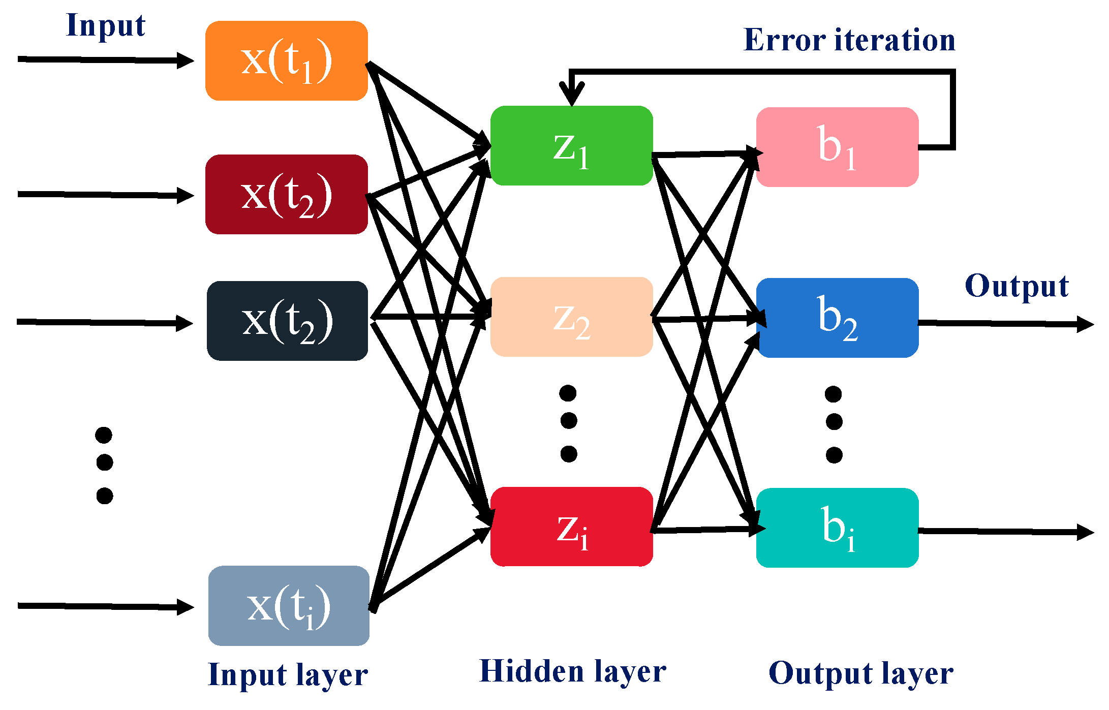
For the nonlinear and fluctuating power of the power grid, artificial neural network algorithms have become an important research means [44]. To improve the prediction accuracy, this paper selects the reverse error propagation neural network to predict the wind and solar power generation. The typical structure is shown in Figure 5. Its functional relationship can be shown by Formula (28).

$$y\left(t\right)=f({\displaystyle \sum }_{i=1}^n{x}_i\left(t\right)z_i\left(t\right)+b_i\left(t\right))$$

(28)

In the formula, x_i(t) is the input sample data set, z_i(t) is the training regulation coefficient in the hidden layer, and b_i(t) is the error value.

The error feedback process is shown in Formulas (29)–(31).

$$E=\Vert \acute{y}\left(t\right)-y{\left(t\right)\Vert }^2$$

(29)

$$z_i\left(t+1\right)=z_i\left(t\right)-{\displaystyle \frac{a\partial E}{\partial w_i\left(t\right)}}$$

(30)

$$b_i\left(t+1\right)=b_i\left(t\right)-{\displaystyle \frac{a\partial E}{\partial b_i\left(t\right)}}$$

(31)

In the formula, E represents the error between the predicted value and the measured value fed back by the reverse transmission, z_i(t + 1) is the coefficient after the learning feedback iteration, and b_i(t) is the error value after the iteration.

The self-learning process of reverse feedback propagation can be shown by Formulas (32) and (33).

$$\Delta w_{km}\left(t\right)=\alpha {\delta }_k\left(t\right)y_m\left(t-1\right)$$

(32)

$${\delta }_k\left(t\right)=-{\displaystyle \frac{\partial E\left(t\right)}{\partial z_k\left(t\right)}}$$

(33)

In the formula, $\Delta w_{km}$ represents the updated weight value.

Hyperparameter optimization is carried out with the aid of Talos and the supported random search tools. MAPE was selected as the standard for quantitatively evaluating the performance of the model.

The hyperparameters of the optimized neural network model are shown in

Table 2. Hyperparameters of the optimized neural network model.

Name of Hyperparameter	Selected Value
The number of neurons	226
Number of hidden layers	3
Learning rate	0.03
Discard rate	4%

.

4. Control Strategies for Cloud–Edge–Device Distribution Networks Combined with Artificial Intelligence

Based on power predictions, the control strategy of the cloud–edge–device distribution network, combined with artificial intelligence, is further obtained. The control strategy aims at minimizing the network loss of the power grid and the regulation cost as the ultimate goal [45]. The network loss of the distribution network is calculated by Formula (34):

$$min{F}_{loss}={\displaystyle \sum }_{t=1}^{96}{\displaystyle \sum }_{i=1}^N{\displaystyle \sum }_{j\in v\left(i\right)}\left({\displaystyle \frac{{\left(P_{ij}^t\right)}^2+{\left(Q_{ij}^t\right)}^2}{{\left(U_i^t\right)}^2}}{r}_{ij}\Delta t\right)$$

(34)

In the formula, F_loss represents network loss; N is the number of nodes in the distribution network; P_ij^t and Q_ij^t represent the active power and reactive power of the ij branch at time t; U_i^t represents the voltage at the i-th node; r_ij^t represents resistance; and Δt represents the time interval, which is 15 min.

The regulation cost of the distribution network can be shown by Formula (35):

$$min{F}_{cost}={\displaystyle \sum }_{t=0}^{95}\left(\begin{array}{c}{\displaystyle {\displaystyle \sum }_{i=1}^{M_1}}\left(C_{tap1}\left|A_{1i}^{t+1}-A_{li}^t\right|\right)+{\displaystyle {\displaystyle \sum }_{i=1}^{M_2}}\left(C_{tap2}\left|A_{2j}^{t+1}-A_{li}^t\right|\right)\\ +{\displaystyle {\displaystyle \sum }_{i=1}^{M_3}}\left(C_{cap}\left|D_k^{t+1}-D_k^t\right|\right)+{\displaystyle {\displaystyle \sum }_{i=1}^{M_4}}\left(C_{svc}\left|E_l^{t+1}-E_l^t\right|\right)\end{array}\right)$$

(35)

In the formula, F_cost represents the cost of power grid regulation; M₁, M₂, M₃, and M₄, respectively, represent the quantities of transformers, voltage regulators, parallel capacitors, and reactive power compensators in the distribution network; and C represents the corresponding equipment cost coefficient.

Under the conditions of meeting customer demands and the safe integration of renewable fluctuating energy, the goal of regulation is to minimize the voltage fluctuation at the node, which can be shown by Formula (36):

$$min{U}_D={\displaystyle \sum }_{t=1}^{24}{\displaystyle \sum }_{t=1}^N{\displaystyle \frac{{\left(U_i-U_N\right)}^2}{{\left(U_{max}-U_{min}\right)}^2}}$$

(36)

In the formula, U_D represents the voltage fluctuation value of the node.

The regulation process still aims at minimizing fluctuations. Therefore, the goal is to minimize the root mean square deviation of the node voltage, which can be shown by Formula (37)

$$min{U}_{RMSE}=\sqrt{{\displaystyle \frac{{{\displaystyle \sum }}_{i=1}^{nr}{\left(U_i-U_{Ni}\right)}^2}{n_r}}}$$

(37)

In the formula, n_r represents the number of nodes in the r-th distribution transformer area; U_l represents the measured voltage value of the l-th node; and U_Ni represents the corresponding set value.

At the same time, the factors influencing the upper and lower node voltages need to be considered to form constraint conditions, as shown in Formula (38):

$$\left\{\begin{array}{c}{P}_l^t=U_l^t{\displaystyle {\displaystyle \sum }_{m=1}^N}{U}_m^t\left(G_{lm}cos{\theta }_{lm}^t+B_{lm}sin{\theta }_{lm}^t\right)\\ Q_l^t=U_m^t{\displaystyle {\displaystyle \sum }_{m=1}^{n_r}}{U}_m^t\left(G_{lm}sin{\theta }_{lm}^t-B_{lm}cos{\theta }_{lm}^t\right)\end{array}\right.$$

(38)

In the formula, P and Q represent active and reactive power, respectively, U represents the voltage variation value, N represents the number of grid nodes, G and B represent the real and imaginary parts of the node admittance matrix, respectively, and ${\theta }_{lm}^t$ represents the angular difference between nodes l and m at time t.

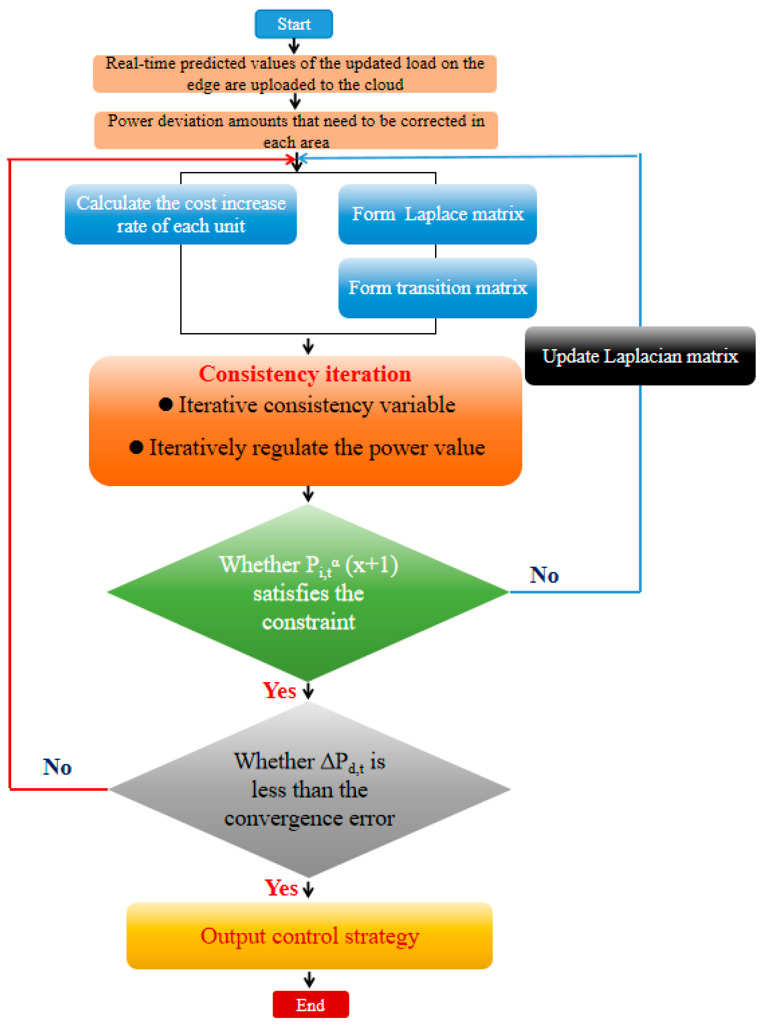
The consistency algorithm has shown good results in distribution optimization [46,47]. In the consistency algorithm, each distribution transformer area is regarded as a node. The Laplacian matrix can accurately reflect the topological structure regulated within each node, as shown by Formula (39):

$$l_{\alpha \beta }=\left\{\begin{array}{c}{\displaystyle {\displaystyle \sum }_{\beta \in n}}{a}_{\alpha \beta },\left(\alpha =\beta \right)\\ -a_{\alpha \beta },\left(\alpha \ne \beta \right)\end{array}\right.$$

(39)

In the formula, l_αβ is the element of the Laplacian matrix, and a_αβ is the non-diagonal element.

d_αβ is the element of the state transition matrix and can be determined through the network topology, as shown in Formula (40):

$$d_{\alpha \beta }={\displaystyle \frac{z_{\alpha \beta }\left(x\right)\left|l_{\alpha \beta }\left(x\right)\right|}{{{\displaystyle \sum }}_{\alpha =1}^n{z}_{\alpha \beta }\left(x\right)\left|l_{\alpha \beta }\left(x\right)\right|}}$$

(40)

In the formula, z_αβ represents the gain control coefficient from node α to node β.

The increase rate of the regulatory cost is the derivative of the regulatory economic cost and the variable power per unit of time. Therefore, the increase rate of the cost after x iterations at time t can be shown by Formula (41):

$${\gamma }_{i,t}^{\alpha }\left(x\right)=\left\{\begin{array}{c}{\displaystyle {\displaystyle \sum }_{\alpha =1}^M}{d}_{\alpha \beta ,t-1}{\gamma }_{i,t-1}^{\beta }+\mu \Delta P_{d,t-1} \Delta P_{i,t-1}>0 \\ {\displaystyle {\displaystyle \sum }_{\alpha =1}^M}{d}_{\alpha \beta ,t-1}{\gamma }_{i,t-1}^{\beta }-\mu \Delta P_{d,t-1} \Delta P_{i,t-1}<0\end{array}\right.$$

(41)

In the formula, μ is the regulation coefficient of power in the virtual power plant.

Then the cost increase rate corresponding to the distribution transformer area can be shown by Formula (42):

$${\gamma }_{i,t}^{\alpha }\left(x\right)={\displaystyle \sum }_{\alpha =1}^M{d}_{\alpha \beta ,t-1}{\gamma }_{i,t-1}^{\beta }$$

(42)

The basis for the termination of the iteration is the deviation of the power after regulation, and its deviation value is expressed by Formula (43)

$$\Delta P_{d,t}=\Delta P_{i,t}-{\displaystyle \sum }_{h=1}^M\Delta P_{i,t}^{\alpha }$$

(43)

In the formula, $\Delta P_{d,t}$ represents the total power deviation of region i in time period t, and $\Delta P_{i,t}$ represents the residual power deviation after regulation.

Based on the cost function and the iterative regulation power function, it can be obtained that the regulation formula which is shown in (44)

$$P_{i,t}^{\alpha }\left(x+1\right)=\left\{\begin{array}{c}{P}_{i,a,min},{\displaystyle \frac{D_a^j\left({\gamma }_{i,t}^{\alpha }\left(x+1\right)-G_j\right)}{2A_j}}\le 0\\ {\displaystyle \frac{D_a^j\left({\gamma }_{i,t}^{\alpha }\left(x+1\right)-G_j\right)}{2A_j}}, 0\le {\displaystyle \frac{D_a^j\left({\gamma }_{i,t}^{\alpha }\left(x+1\right)-G_j\right)}{2A_j}}\le P_{i,a,min}\\ P_{i,a,min},{\displaystyle \frac{D_a^j\left({\gamma }_{i,t}^{\alpha }\left(x+1\right)-G_j\right)}{2A_j}}\ge P_{i,a,min}\end{array}\right.$$

(44)

In the formula, P_i,t^α(x + 1) represents the control power of the x + 1 iteration of the α-th control unit in the distribution transformer area i at time t.

In the calculation of the consistency algorithm, when the deviation of the power is less than the convergence error, it indicates that the calculation of the consistency algorithm is completed. The cost increase rate is iteratively calculated again until the cost increase rates of different nodes are at the same position, as shown in Formula (45)

$${\displaystyle \frac{\partial C_{i,t,k_4^i}^4}{\partial P_{i,t,k_4^i}^4}}=\cdots ={\displaystyle \frac{\partial C_{i,t,k_4^i}^4}{\partial P_{i,t,k_4^i}^4}}$$

(45)

In the formula, superscript 4 represents the load that can be directly controlled.

Finally, the optimal value of the regulation power when the regulation cost is minimized is obtained, as shown in Formula (46)

$$P_{i,t}^{{\alpha }^{*}}={\displaystyle \frac{D_a^j\left({\gamma }_{i,t}^{{\alpha }^{*}}-G_j\right)}{2A_j}}$$

(46)

In the formula, $P_{i,t}^{{\alpha }^{*}}$ represents the optimal regulation power value.

MATLAB R2018a software is adopted to develop a resource aggregation scheduling and optimization control model. Figure 6 shows the solution process of the consistent distributed optimization control.

5. Results and Discussion

From the perspective of electricity consumption, the changes in active power and reactive power are not random but have a certain regularity. Among them, the start-up and shutdown of equipment are separately classified as a cluster. The six characteristics of the derivatives of three-phase active power and reactive power are used to divide the data cluster, and the cluster characteristics are shown in Figure 7. The relationship between active and reactive power is distinctive for specific types of devices. In Figure 7, the horizontal coordinates P₁ to P₆, respectively, represent the three-phase active and three-phase reactive power.

As shown in Figure 7, the six clusters have distinct characteristics. Clusters 1, 3, and 5 exhibit an increase in the power of one phase, while the other clusters, 2, 4, and 6, can be regarded as a collection of three-phase connected devices. The relationship between active power and reactive power has also been clearly revealed. Clusters 1, 3, and 5 do not have an increase in reactive power when the equipment is turned on, while clusters 4 and 6 show a significant upward trend. In cluster 4, the reactive power is even higher than the active power.

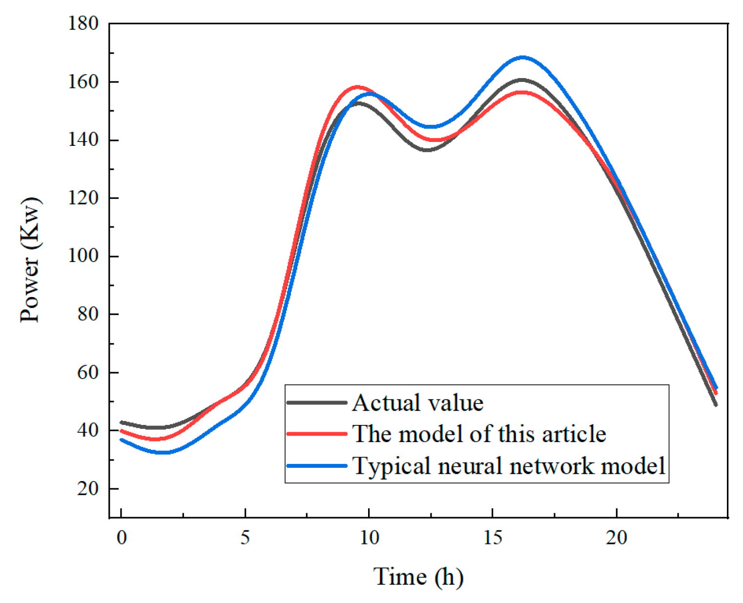
The electricity consumption model proposed in this paper is compared with the typical neural network model. For comparison, a multi-layer perceptron is selected as the typical neural network model. Figure 8 shows the comparison curves of the predicted values and actual values. As can be seen from Figure 8, the load variation at the customer end throughout the day shows a situation of being high during the day and low at night, which is in line with people’s daily living habits. The model developed based on artificial neural networks can well-follow the changes in load. However, compared with the absolute error value of the actual value, its accuracy is not as good as that of the model proposed in this paper. This is mainly because typical neural network models do not consider sudden changes in load. In the research of scholars, this method has shown a certain feasibility. However, in the case of significant fluctuations (the start or stop of the devices), the accuracy is just satisfactory. The model proposed in this paper makes up for this shortcoming very well.

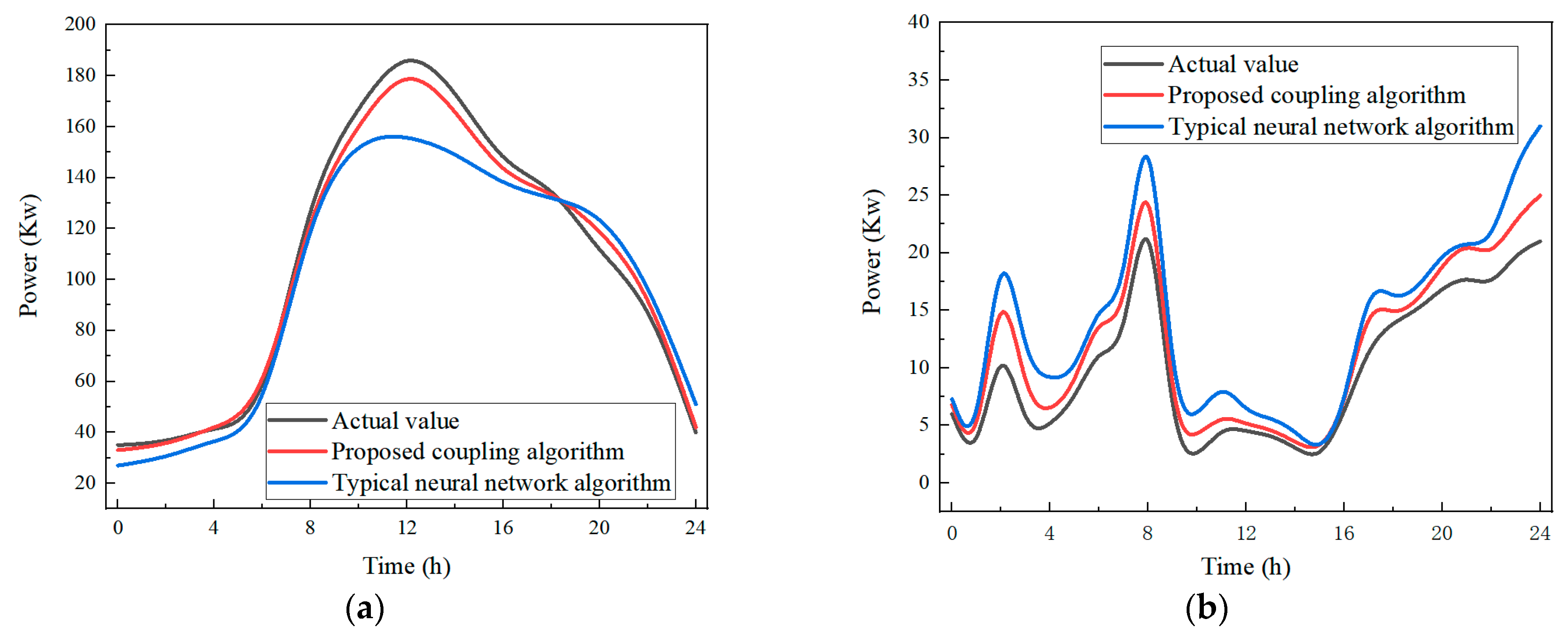
Short-term forecasting of solar and wind power generation provides key guidance for grid regulation. This paper proposes a method of coupling long and short memory with error feedback correction to predict solar and wind power generation. Meanwhile, the proposed coupling prediction algorithm is compared with the traditional neural network algorithm. Figure 9 shows the comparison between the predicted power curves of different algorithms and the actual power curves in a typical day. A typical day refers to a day randomly selected without extreme weather (such as snowstorm, sandstorm, rainstorm, etc.). It can be seen from Figure 9a that, within a typical day, the solar power generation shows obvious fluctuations, which is related to the constantly changing weather. And the power shows a trend of increasing first and then decreasing, reaching the maximum power generation capacity at noon. The solar radiation intensity is the strongest at noon and the lowest in the morning and evening. The absolute value of the difference between the predicted value and the actual value is significantly smaller than that of the neural network algorithm, which indicates that the proposed coupling algorithm has better accuracy. It can be known from the analysis of Figure 9b that the wind power generation also has obvious fluctuations. At noon, the wind speed is relatively low, and the wind power generation capacity is also small. In the morning and evening, when the wind speed is relatively high, the wind power generation capacity is also correspondingly large. The proposed coupling algorithm and neural network algorithm have a good description of the volatility of solar and wind power generation. In a vertical comparison, the proposed coupling algorithm can better approach the actual value, and its prediction accuracy is higher.

To evaluate the performance of the proposed coupling algorithm, MAPE, root mean square error (RMSE), mean absolute error (MAE), and coefficient of determination (R²) are used to measure the performance. The calculation formulas of the performance indicators are shown as (3), (47)–(49):

$$\mathrm{RMSE}=\sqrt{\left({\displaystyle \frac{1}{N}}{\displaystyle \sum }_i^N{\left(Y_i-Y_i^{\prime }\right)}^2\right)}$$

(47)

$$\mathrm{MAE}={\displaystyle \frac{1}{N}}{\displaystyle \sum }_i^N\left|Y_i-Y_i^{\prime }\right|$$

(48)

$$R^2=1-{\displaystyle \frac{{{\displaystyle \sum }}_{n=1}^N{\left(Y_i-{\widehat{Y}}_i\right)}^2}{{{\displaystyle \sum }}_{n=1}^N{\left(Y_i-\widehat{Y}\right)}^2}}$$

(49)

Table 3. Performance comparison of each algorithm.

Algorithm	RMSE	MAPE	MAE	R2
SVR	1454.8	6.07	238.5	0.968
KM-Reg	1362.2	5.59	202.4	0.978
GMM-Reg	1426.1	5.73	228.1	0.981
Neural network algorithm	1410.1	5.64	211.2	0.986
Proposed coupling algorithm	1347.2	5.36	199.4	0.991

summarizes the performance comparison between the proposed coupling algorithm and the traditional algorithms. SVR, KM-Reg, GMM-Reg, and neural network are typical artificial intelligence algorithms. KM-Reg is an improvement of the KM model, mainly by introducing dependency equations and regularization parameters to correct the model. GMM-Reg is an improved algorithm that combines the Gaussian mixture model with regularization techniques. In the process of proposing the coupling algorithm, 85% of the data was used as the training set, and 15% of the data was used as the testing set. For the four typical algorithms, the same training set and testing set are adopted to regulate the algorithm coefficients, thereby obtaining the electric power prediction algorithm. It can be known from Table 3 that the proposed coupling algorithm has the best performance indicators. Among them, the value of R² reaches 0.991, which indicates that the proposed coupling algorithm has good linear correlation performance. Meanwhile, the values of RMSE are 1347.2, MAPE are 5.36, and MAE are 199.4. The three error indicators are the lowest values of each algorithm. This also indicates that the proposed coupling algorithm has good accuracy.

Rushdi et al. [48] used a linear regression model to predict the power generation of wind power, with an R² coefficient of only 0.836. Therefore, the model was improved, and a combination of second-order polynomial regression and artificial neural network was adopted for power prediction. The results showed that the R² coefficient could reach 0.997. However, it should be noted that this model made accurate predictions when there were sufficient computing resources. Wang et al. [49] proposed an algorithm that combines feature selection with long- and short-term time series networks to predict the power of wind and solar power. In the long short-term time series network, the long short-term memory method and the bidirectional long short-term memory method were selected. In feature selection, Random Forest, Grey Relational Analysis, and Principal Component Analysis were chosen. By comparing different combinations, it was found that the bidirectional long short-term memory method combined with random forest had the lowest error. The MAPE value could reach 5.16, while the MAPE values of the other combined algorithms were all above 6. An improved long short-term memory method is obtained in combination with error feedback correction in this paper, which can reduce installation and computing costs. Moreover, its R² value reaches 0.991, and the MAPE value can reach 5.36. While saving computing resources, it ensures the prediction accuracy.

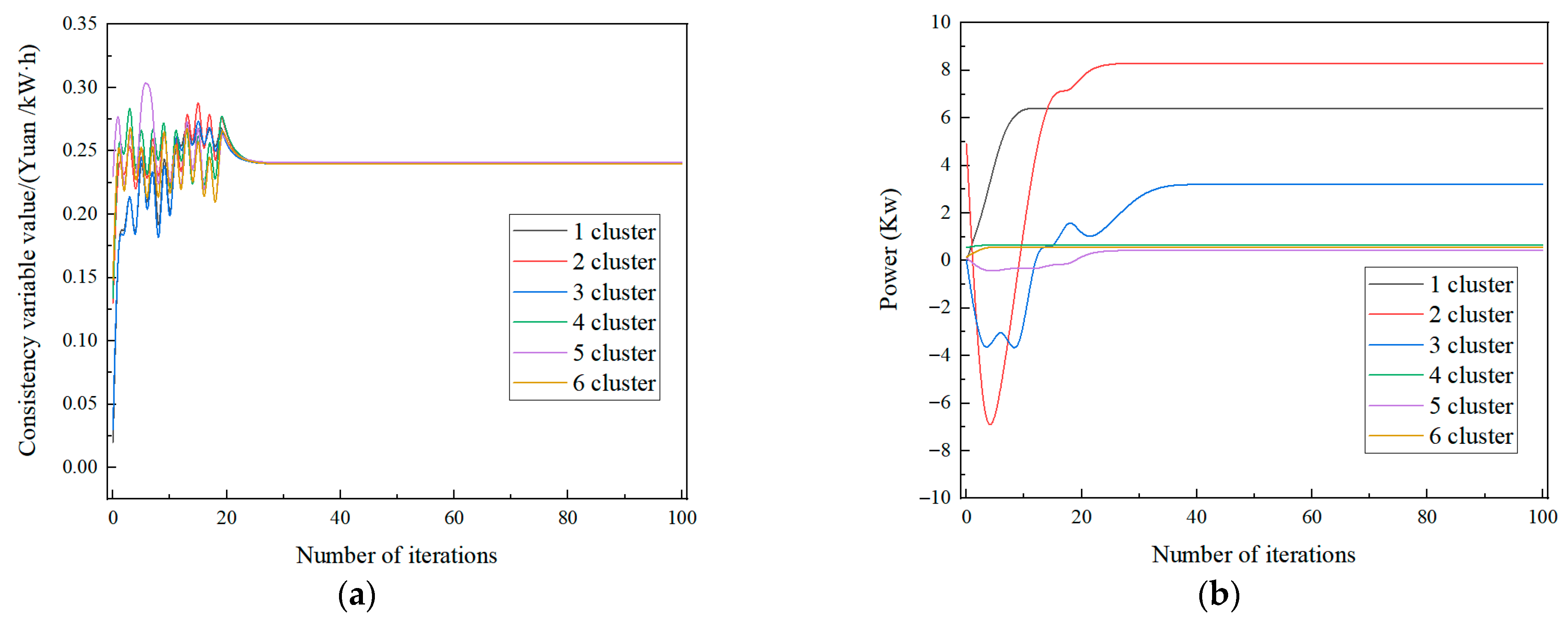
The electricity consumption and the wind and solar power generation have been taken into account, but the power prediction cannot completely eliminate the errors. Under the new energy situation, the distribution regulation and control of cloud-edge-device distribution networks, combined with artificial intelligence, is particularly important. A consistent distributed intelligent optimization is adopted to regulate and control the distribution network. When a certain transformer area needs to correct the power deviation of 32.15 kW, Figure 10 depicts the cost escalation rates per cluster alongside power consistency convergence.

It can be known from Figure 10a that the costs of each cluster are different at the beginning, but basically can reach a stable state after 25 iterations, with a cost increase rate of CNY 0.241/kW·h. When the increasing rate of the regulation cost is stable, the optimal regulation powers of each cluster are 6.42, 8.3, 3.21, 0.67, 0.43, and 0.58 Kw, respectively. The regulation and control all meet the conditions of operational constraints. It can be seen that, in the face of the variable electricity consumption and the fluctuating input of new energy, the distributed coevolution model of the cloud–edge–device power grid structure, combined with artificial intelligence, can effectively achieve low-cost regulation and control.

6. Conclusions

The gradual replacement of fossil energy by clean renewable energy is the key to the current energy structure transformation. However, diverse electricity consumption combined with the large-scale integration of renewable energy will lead to more frequent voltage fluctuations in the power grid, so higher requirements have been put forward for the operation of the power grid. At present, both centralized and decentralized pressure regulation methods require a large amount of computing resources to accurately predict fluctuating loads, so as to make adjustments. However, with the development of artificial intelligence and cloud computing, the processing of huge databases and the release of computing resources have become possible. A cloud–edge–device collaborative framework is developed. According to the energy consumption situation at the customer end, this paper effectively combines load monitoring with power prediction. A new method for electricity consumption analysis based on the mixture of traditional mathematical statistics and machine-learning methods is proposed to make up for the deficiencies of non-intrusive load detection methods. Aiming at problems such as overfitting and the demand for accurate short-term renewable power generation prediction, it is proposed to adopt the long short-term memory method to fix data information and combine the error feedback to develop a hybrid model to obtain the prediction of renewable power generation under the collaboration of cloud–edge–device. Power prediction cannot completely eliminate errors. Combined with the consistency algorithm to construct the regulation strategy. Finally, the cloud–edge–device distributed coevolution model of the power grid is obtained to achieve the economy and security of power grid voltage control.

References

1. Yao, Z.T.; Ji, X.S.; Sarker, P.K.; Tang, J.H.; Ge, L.Q.; Xia, M.S.; Xi, Y.Q. A comprehensive review on the applications of coal fly ash. Earth-Sci. Rev. 2015, 141, 105–121. [Google Scholar] [CrossRef]
2. Yuan, Q.X.; Yang, G.; Zhang, Y.S.; Wang, T.; Wang, J.W.; Romero, C.E. Supercritical CO2 coupled with mechanical force to enhance carbonation of fly ash and heavy metal solidification. Fuel 2022, 315, 123154. [Google Scholar] [CrossRef]
3. Cao, Y.F.; Liang, S.L.; Chen, X.N.; He, T.; Wang, D.D.; Cheng, X. Enhanced wintertime greenhouse effect reinforcing Arctic amplification and initial sea-ice melting. Sci. Rep. 2017, 7, 8462. [Google Scholar] [CrossRef]
4. Yuan, Q.X.; Zhang, Y.S.; Wang, T.; Wang, J.W.; Romero, C.E. Mineralization characteristics of coal fly ash in the transition from non-supercritical CO2 to supercritical CO2. Fuel 2022, 318, 123636. [Google Scholar] [CrossRef]
5. Yuan, Q.X.; Lu, H.R.; Guo, X.M.; Ma, S.X. Quantitative effects of physical encapsulation during carbonation process based on scaled up simulation of fly ash particles. J. Energy Inst. 2024, 115, 10167. [Google Scholar] [CrossRef]
6. Jiang, T.Y.; Guo, Q.M.; Yu, J.H.; Jahanger, A.; Yu, Y.; Li, X.L. Spatial mismatch of resources in China under the “dual-carbon” goal: A new perspective incorporating energy and environmental factors. Energy 2025, 320, 135297. [Google Scholar] [CrossRef]
7. Xing, Y.Z.; Zhang, X.Y.; Li, D.X.; Xue, J.X.; Cao, J.Y.; Zhang, R. Carbon emission reduction responsibility allocation in China’s power generation sector under the “dual carbon” target—Based on a two-stage shared responsibility approach. J. Clean. Prod. 2025, 489, 144699. [Google Scholar] [CrossRef]
8. Zhang, J.; Hodge, B.M.; Lu, S.Y.; Hamann, H.F.; Lehman, B.; Simmons, J.; Campos, E.; Banunarayanan, V.; Black, J.; Tedesco, J. Baseline and target values for regional and point PV power forecasts: Toward improved solar forecasting. Sol. Energy 2015, 122, 804–819. [Google Scholar] [CrossRef]
9. Wang, Y.; Zou, R.M.; Liu, F.; Zhang, L.J.; Liu, Q.Y. A review of wind speed and wind power forecasting with deep neural networks. Appl. Energy 2021, 304, 117766. [Google Scholar] [CrossRef]
10. Pedersen, L.; Stang, J.; Ulseth, R. Load prediction method for heat and electricity demand in buildings for the purpose of planning for mixed energy distribution systems. Energy Build. 2008, 40, 1124–1134. [Google Scholar] [CrossRef]
11. Hai, V.T.; Anh, V.T.; Tan, M.P.; Thang, T.N. Minimize the One-Year Energy for Distribution Power Grids With Renewable Energies-Based Distributed Generators, Capacitors, and Soft Open Points. Int. J. Energy Res. 2015, 1, 3457520. [Google Scholar]
12. Karthik, N.; Arul, R.; Mohit, B.; Valliappan, R.; Vojtech, B.; Lukas, P. Improved Lyrebird optimization for multi microgrid sectionalizing and cost efficient scheduling of distributed generation. Sci. Rep. 2025, 15, 17345. [Google Scholar] [CrossRef]
13. Amal, K.A.; Mohammed, A.; Rakan, A.; Nazir, A.; Sultan, A.; Othman, A.; Ali, A.; Hassan, A. Mitigating malicious denial of wallet attack using attribute reduction with deep learning approach for serverless computing on next generation applications. Sci. Rep. 2025, 15, 18720. [Google Scholar] [CrossRef] [PubMed]
14. Zahra, K.M.; Mehdi, F.; Javad, A.T. An energy-aware virtual machine placement method in cloud data centers based on improved Harris Hawks optimization algorithm. Computing 2025, 107, 136. [Google Scholar]
15. Saurabh, V.; Gordhan, J. Elevating manufacturing excellence with multilevel optimization in smart factory cloud computing using hybrid model. Clust. Comput. 2025, 28, 342. [Google Scholar] [CrossRef]
16. Tran, D.; Khambadkone, A.M. Energy management for lifetime extension of energy storage system in micro-grid applications. IEEE Trans. Smart Grid 2013, 4, 1289–1296. [Google Scholar] [CrossRef]
17. Brucke, K.; Arens, S.; Telle, J.-S.; Steens, T.; Hanke, B.; von Maydell, K.; Agert, C. A non-intrusive load monitoring approach for very short-term power predictions in commercial buildings. Appl. Energy 2021, 292, 116860. [Google Scholar] [CrossRef]
18. Brucke, K.; Arens, S.; Telle, J.-S.; SunkeSchlüters; Hanke, B.; von Maydell, K.; Agert, C. Particle Swarm Optimization for Energy Disaggregation in Industrial and Commercial Buildings. arXiv 2006, arXiv:2006.12940. [Google Scholar]
19. Welikala, S.; Dinesh, C.; Ekanayake, M.P.B.; Godaliyadda, R.I.; Ekanayake, J. Incorporating appliance usage patterns for non-intrusive load monitoring and load forecasting. IEEE Trans. Smart Grid 2017, 10, 448–461. [Google Scholar] [CrossRef]
20. Wurm, M.; Coroama, V.C. Grid-level short-term load forecasting based on disaggregated smart meter data. Comput. Sci.-Res. Dev. 2018, 33, 265–266. [Google Scholar] [CrossRef]
21. Gopakumar, S.; Sree, R.R.T. Determination of Power Transformer Fault’s Severity Based on Fuzzy Logic Model with GR, Level and DGA Interpretation. J. Electr. Eng. Technol. 2023, 19, 2527–2548. [Google Scholar] [CrossRef]
22. Hossain, R.R.; Yin, T.; Du, Y.; Huang, R.; Tan, J.; Yu, W.; Liu, Y.; Huang, Q.H. Efficient learning of power grid voltage control strategies via model-based deep reinforcement learning. Mach. Learn. 2023, 113, 2675–2700. [Google Scholar] [CrossRef]
23. Fan, G.-F.; Peng, L.-L.; Hong, W.-C. Short term load forecasting based on phase space reconstruction algorithmand bi-square kernel regression model. Appl. Energy 2018, 224, 13–33. [Google Scholar] [CrossRef]
24. Wang, K.; Xu, C.; Zhang, Y.; Guo, S.; Zomaya, A. Robust big data analytics for electricity price forecasting in the smart grid. IEEE Trans. Big Data 2017, 5, 34–45. [Google Scholar] [CrossRef]
25. Fan, S.-K.S.; Su, C.-J.; Nien, H.-T.; Tsai, P.-F.; Cheng, C.-Y. Using machine learning and big data approaches to predict travel time based on historical and real-time data from Taiwan electronic toll collection. Soft Comput. 2017, 22, 5707–5718. [Google Scholar] [CrossRef]
26. Guo, J.R.; Dou, C.X.; Yue, D.; Zhang, B.; Zhang, Z.J.; Zhang, Z.Q. Cloud-edge-end collaboration-based joint design of frequency control and transmission communication for virtual power plants. Int. J. Electr. Power Energy Syst. 2025, 166, 110564. [Google Scholar] [CrossRef]
27. Li, H.; Wu, Z.R.; Liu, Y.H.; Luo, J.L.; Yang, K.P. Overall architecture design of power IoT transmission scenario based on cloud-edge-end collaboration. J. Phys. Conf. Ser. 2025, 2935, 012021. [Google Scholar] [CrossRef]
28. Li, J.R.; Li, X.Y.; Yuan, J.; Li, G.Z. Load Balanced Data Transmission Strategy Based on Cloud–Edge–End Collaboration in the Internet of Things. Sustainability 2022, 14, 9602. [Google Scholar] [CrossRef]
29. Azgomi, H.; Sohrabi, M.K. MR-MVPP: A map-reduce-based approach for creating MVPP in data warehouses for big data applications. Inf. Sci. 2021, 570, 200–224. [Google Scholar] [CrossRef]
30. Min, Y.; Chaoran, W.; Yi, L.; Gustaf, O.; Hua, B. Water and related electrical energy use in urban households-Influence of individual attributes in Beijing, China. Resour. Conserv. Recycl. 2018, 130, 190–199. [Google Scholar]
31. Muyuan, C. Building molecular model series from heterogeneous CryoEM structures using Gaussian mixture models and deep neural networks. Commun. Biol. 2025, 8, 798. [Google Scholar] [CrossRef]
32. Chen, Y.J.; Cheng, N.; Cai, M.; Cao, C.Z.; Yang, J.W.; Zhang, Z.C. A spatially constrained asymmetric Gaussian mixture model for image segmentation. Inf. Sci. 2021, 575, 41–65. [Google Scholar] [CrossRef]
33. Alexander, R. Modified Bayesian Information Criterion for Item Response Models in Planned Missingness Test Designs. Analytics 2024, 3, 449–460. [Google Scholar] [CrossRef]
34. Shota, S.; Shun, S.; Hiroki, S.; Takama, Y. Dynamic Generation of Subordinate Clusters Based on Bayesian Information Criterion for Must-Link Constrained K-Means:Regular Papers. J. Adv. Comput. Intell. Intell. Inform. 2024, 28, 86–93. [Google Scholar]
35. Shinotsuka, H.; Nagata, K.; Yoshikawa, H.; Mototake, Y.; Shouno, H. Development of spectral decomposition based on Bayesian information criterion with estimation of confidence interval. Sci. Technol. Adv. Mater. 2020, 21, 402–419. [Google Scholar] [CrossRef]
36. Tu, B.E.; Xu, X.L.; Gu, Y.F.; Deng, K.T.; Xu, Y.L.; Zhang, T.Y.; Gao, X.R.; Wang, K.N.; Wei, Q.J. Improved Droop Control Strategy for Islanded Microgrids Based on the Adaptive Weight Particle Swarm Optimization Algorithm. Electronics 2025, 14, 893. [Google Scholar] [CrossRef]
37. Udit, M.; Indra, K.; Ramakrishna, G.; Priyam, G.; Nithesh, N. Artificial intelligence based hybrid solar energy systems with smart materials and adaptive photovoltaics for sustainable power generation. Sci. Rep. 2025, 15, 17370. [Google Scholar] [CrossRef]
38. Ginzburg-Ganz, E.; Horodi, E.D.; Shadafny, O.; Savir, U.; Machlev, R.; Levron, Y. Statistical Foundations of Generative AI for Optimal Control Problems in Power Systems: Comprehensive Review and Future Directions. Energies 2025, 18, 2461. [Google Scholar] [CrossRef]
39. Pal, B.; Theodoros, E. Artificial intelligence to support the integration of variable renewable energy sources to the power system. Appl. Energy 2021, 290, 116754. [Google Scholar] [CrossRef]
40. Eugenia, P.; Lucas, V.; Marius, P. Clear sky solar irradiance models derived through interdependent parameterization. Renew. Energy 2025, 250, 123371. [Google Scholar] [CrossRef]
41. Bhola, K.R.; Chandramohan, V.P. A numerical study for estimating dynamic performance parameters of 40 × 40 mm2 ultrasonic piezoelectric micro blower and proposing a set of dimensions for optimum performance. Energy 2025, 314, 134198. [Google Scholar]
42. Moradzadeh, A.; Zakeri, S.; Shoaran, M.; MohammadiIvatloo, B.; Mohamamdi, F. Short-Term Load Forecasting of Microgrid via Hybrid Support Vector Regression and Long Short-Term Memory Algorithms. Sustainability 2020, 12, 7076. [Google Scholar] [CrossRef]
43. Ji, X.; Lu, C.X.; Xie, B.M.; Guo, H.Y.; Zheng, B.Y. Combination of a Rabbit Optimization Algorithm and a Deep-Learning-Based Convolutional Neural Network–Long Short-Term Memory-Attention Model for Arc Sag Prediction of Transmission Lines. Electronics 2024, 13, 4593. [Google Scholar] [CrossRef]
44. Chen, H.W.; Liu, S.M.; Magomedov, R.M.; Davidyants, A.A. Optimization of inflow performance relationship curves for an oil reservoir by genetic algorithm coupled with artificial neural-intelligence networks. Energy Rep. 2021, 7, 3116–3124. [Google Scholar] [CrossRef]
45. He, Y.; Li, Z.T.; Zhang, J.; Shi, G.Y.; Cao, W.P. Day-ahead and intraday multi-time scale microgrid scheduling based on light robustness and MPC. Int. J. Electr. Power Energy Syst. 2022, 144, 108546. [Google Scholar] [CrossRef]
46. Lin, L.; Sun, T.; Fan, M.; You, F.R.; Huang, Y.M. An adaptive power-voltage hierarchical control based on improved consensus algorithm for DC traction power supply system. Electr. Power Syst. Res. 2025, 245, 111642. [Google Scholar] [CrossRef]
47. Quan, Y.; Xi, L. Smart generation system: A decentralized multi-agent control architecture based on improved consensus algorithm for generation command dispatch of sustainable energy systems. Appl. Energy 2024, 365, 123209. [Google Scholar] [CrossRef]
48. Rushdi, M.A.; Yoshida, S.; Watanabe, K.; Ohya, Y.; Ismaiel, A. Deep Learning Approaches for Power Prediction in Wind-Solar Tower Systems. Energies 2024, 17, 3630. [Google Scholar] [CrossRef]
49. Wang, H.; Fu, W.Y.; Li, C.; Li, B.; Cheng, C.; Gong, Z.H.; Hu, Y.L. Short-Term Wind and Solar Power Prediction Based on Feature Selection and Improved Long- and Short-Term Time-Series Networks. Math. Probl. Eng. 2023, 1, 7745650. [Google Scholar] [CrossRef]
Figure 1. Specific distributed collaborative framework of the cloud-edge-device distribution network.
Mathematics 13 02924 g001
Figure 2. The structure of the customer-side electricity consumption prediction algorithm.
Mathematics 13 02924 g002
Figure 3. Algorithm structure.
Mathematics 13 02924 g003
Figure 4. The structure of the renewable power generation prediction.
Mathematics 13 02924 g004
Figure 5. Structure of typical artificial neural network algorithms.
Mathematics 13 02924 g005
Figure 6. Solution process of the consistent distributed optimization control.
Mathematics 13 02924 g006
Figure 7. Power derivatives of all features in the six clusters.
Mathematics 13 02924 g007
Figure 8. Comparison curves of the predicted values and actual values.
Mathematics 13 02924 g008
Figure 9. Comparison between the predicted power curves of different algorithms and the actual power curves in a typical day. (a) Wind power generation; (b) Solar power generation.
Mathematics 13 02924 g009
Figure 10. Process of cost increase rate of each cluster and convergence of power consistency. (a) Cost increase rate; (b) Power consistency.
Mathematics 13 02924 g010