A Novel Method for Virtual Real-Time Cumuliform Fluid Dynamics Simulation Using Deep Recurrent Neural Networks

Abstract

The real-time simulation of atmospheric clouds for the visualisation of outdoor scenarios has been a computer graphics research challenge since the emergence of the natural phenomena rendering field in the 1980s. In this work, we present an innovative method for real-time cumuli movement and transition based on a Recurrent Neural Network (RNN). Specifically, an LSTM, a GRU and an Elman RNN network are trained on time-series data generated by a parallel Navier–Stokes fluid solver. The training process optimizes the network to predict the velocity of cloud particles for the subsequent time step, allowing the model to act as a computationally efficient surrogate for the full physics simulation. In the experiments, we obtained natural-looking behaviour for cumuli evolution and dissipation with excellent performance by the RNN fluid algorithm compared with that of classical finite-element computational solvers. These experiments prove the suitability of our ontogenetic computational model in terms of achieving an optimum balance between natural-looking realism and performance in opposition to computationally expensive hyper-realistic fluid dynamics simulations which are usually in non-real time. Therefore, the core contributions of our research to the state of the art in cloud dynamics are the following: a progressively improved real-time step of the RNN-LSTM fluid algorithm compared to the previous literature to date by outperforming the inference times during the runtime cumuli animation in the analysed hardware, the absence of spatial grid bounds and the replacement of fluid dynamics equation solving with the RNN. As a consequence, this method is applicable in flight simulation systems, climate awareness educational tools, atmospheric simulations, nature-based video games and architectural software.

1. Introduction

The realistic simulation of physical effects is computationally expensive in some cases, especially when it comes to solving differential equations in a multidimensional space. These simulations are widely used in engineering and science, where accuracy is more important than the time it takes to produce the solution. For example, these methods can be used to simulate complex behaviours in physics [1] and for the analysis of fluids [2].

These physical models are also very convenient in terms of providing real-world gaming experiences in interactive applications, such as computer games and simulators [3]. In this case, real-time execution is more important than accuracy, provided that the result is still realistic. However, achieving real-time solving of the equations can be prohibitively expensive, which reduces the addressable market of these applications.

This paper addresses the real-time simulation of 3D atmospheric clouds for computer games, which has been a relevant challenge for decades, as revealed in the [4,5] surveys.

To this end, and to perform cloud computer simulations, there are currently two possible approaches for the generation of these gaseous entities as stated by [6]: ontogenetics and physically based methods. The first type (ontogenetics) means that a mathematical abstraction is used to simplify the complexity of meteorological physics to simulate clouds, which usually works in real time, such as reported in the works of [7,8], which are for computer games.

In contrast, the second type (physically based) implements precise physical simulation models of cloud processes to produce accurate and hyper-realistic results at the expense of computational efficiency, which often implies non-real-time results, such as the studies by [9] for computer games and [10] for movies, both of which improved the cloud radiometry. However, both approaches are resource intensive and require the use of graphics processing units (GPUs) to achieve efficiency in environments that are intended to be used in real-time simulation.

A particular application of differential equation solving in volumetric space is the computer simulation of cloud dynamics. Since air and water vapour behave as fluids, their dynamic behaviour can be modelled using the Navier–Stokes equations (NSEs). For this reason, they are solved by numerical methods that use finite-element structures rather than analytically. Despite the numerous improvements intended to increase the simulation speed, particularly the execution on GPUs, it is still challenging to execute this process on reasonably priced hardware.

An alternative approach involves using the output of multiple fluid simulations to train a surrogate model based on neural networks (NNs), as deep learning provides a good approximation for multidimensional nonlinear outcomes efficiently. Ref.  [11] demonstrates the use of deep learning algorithms with artificial neural networks and shows how they can predict input parameters in computational fluid dynamics, reducing computational costs and improving accuracy. More recent studies demonstrating the application of neural networks and deep learning methods for the simulation of fluid dynamics include the works of [12,13,14]. This approach is also explored in this work, which involves replacing the parallel Navier–Stokes fluid solver with a recurrent neural network previously trained with multiple simulations in an engine to emulate the dynamics of clouds in real time. Thus, our method employs only such an RNN, as illustrated in the layout summary of the proposal in Figure 1 to animate cumuliforms. Compared with numerical methods for solving the Navier–Stokes equations, the use of this approach provides a substantial enhancement in speed and eliminates the need for spatial grid bounds, increasing the overall computing power. While RNNs have been used to simulate blood movement [15], heat propagation [16] and turbulence prediction [17], to our knowledge, RNNs have not been used for simulating cloud dynamics to date.

The scope of our method is not limited to the simulation of cloud dynamics and it could be applied to other similar complex physical systems like fire, twisters, waves, birds, etc. The speed-up gains obtained by means of the application of this surrogate model release resources for additional processing on the General-Purpose Graphics Processing Units (GPGPUs). This research proposes an approach that can run on entry-level graphic hardware with low computational cost and minimum energy consumption for flight simulation, virtual reality featuring outdoor scenes, architectural software, digital cultural heritage and nature-based computer games.

Therefore, the contributions of our research work to the state of the art of cloud motion are as follows:

• New method that replaces a Navier–Stokes fluid solver with a Recurrent Neural Network.
• Better constant real-time performance by the RNN fluids algorithm as compared to the previous literature.
• Near-optimal performance in cloud dynamics prediction by using deep RNNs.
• Natural cumuli behaviour in real-time irrespective of the 3D grid dimensions.
• Novel approach to simulate other complex physical processes with neural networks.

In summary, this paper is organised as follows: Section 2 presents related works on cloud dynamics simulations and the methods that have been developed to date, while Section 3 explains the theoretical background for our cloud rendering method and the previous model for the replacement of the Navier–Stokes fluid solver. Section 4 presents the proposed deep learning RNN structure and dataset used for the training phase, and Section 5 describes the two experiments and the performance results obtained during the RNN inferences. Section 6 presents the discussions and factual limitations related to the current proposed model, and finally, Section 7 proposes possible future work and improvements.

2. Related Works

As mentioned in the previous section, there are two methods for cloud simulation: ontogenetics and physically based methods. A summary of the capabilities of each approach is presented in

Table 1. Features per study of some recent and significant related works.

Author	[20]	[27]	[10]	[8]
Procedural	✗	✓	✓	✓
Cloud dynamics	✓	✗	✗	✓
Traverse	✓	✗	✗	✓
Interactive	✓	✓	✗	✓
Manoeuvring around	✓	✗	✓	✓
All kinds of clouds	✗	✓	✗	✓
Realism	✗	✓	✓	✓
Real-time performance	✓	✓	✗	✓
State of the art	✗	✓	✓	✓
Generation method	Particle systems	Texturised skydome	Neural networks	Ray casting
Simulation approach	Ontogenetic	Ontogenetic	Physically based	Ontogenetic

. Notably, some outstanding works on cloud dynamics have paved the way for the present research. Ref. [18] presented a new method called the coupled map lattice (CML), which extends a cellular automaton to simulate cloud dynamics. The drawbacks of this method are a constrained fluid grid size and rendering time steps from 3 to 30 s. Ref. [19] proposed an improved method for simulating cloud formation on the basis of an efficient computational Navier–Stokes fluid solver; they combined a Navier–Stokes fluid solver with a model of the natural processes of cloud formation, including the buoyancy, relative humidity and condensation. Ref. [20] developed a particle system model to render cumuliform clouds while introducing impostors as a feature to improve the speed. The author also developed a cloud dynamics simulation based on the Euler equations of incompressible fluid, the water continuity equation and the thermodynamic equation. Both [19,20] were limited to a 3D lattice for cloud dynamics, and their rendering methods are not considered state of the art. Ref. [21] proposed a simple method for controlling cumuliform cloud simulations that can generate clouds with desired shapes specified by the user. In this method, the cloud formation process is controlled by a feedback controller, and the external forces are calculated by the geometric potential field. This method was constrained by a grid size of 320 × 80 × 100 and rendering time steps starting at 7 s. Ref. [22] proposed an approach similar to that of [23] but with accelerated particle system simulation by multicore and multithread hardware techniques. Currently, particle systems are no longer state of the art for cloud rendering. The work of [8] demonstrated the use of explicit and implicit parallel programming techniques for volumetric cloud rendering and dynamics to achieve an optimum balance between realism and performance. The principle that guides this work is real-time cloud rendering using efficient algorithms that can run on standard computers with modest GPGPUs by conforming to the clouds with pseudo-spheroidal primitives. One of its main contributions is a programming framework that can be reused in the education field or software industry for real-time cloud simulation of outdoor scenarios. However, for cloud dynamics, it also employs a 3D grid volume that underpins the performance achieved in this work. Ref. [24] proposed an efficient, physics-based procedural model for real-time animation and visualisation of cumulus clouds at the landscape scale. The authors coupled a coarse Lagrangian model for air parcels with procedural amplification by using volumetric noise. Finally, an article by [25] proposed a novel model to simulate thermodynamic systems, such as cloud dynamics, by using a 2D cellular automaton that is oriented to satellite images; therefore, it cannot be compared with other 3D approaches. Additionally, ref. [26] generated cumuli, strati, and stratoscumuli as well as realistic formations caused by changes in the atmosphere to simulate large-scale cloud super-cell clusters of cumulonimbus formations. The model also enables the efficient exploration of stormscapes with a lightweight set of high-level parameters that explore cloud formations and dynamics. This method is limited by the grid size and cannot simulate long cumuli transition across a wide space.

To avoid the fluid grid restrictions of previous works, a new approach is needed. Deep neural networks (DNNs) are considered approximators of universal functions and can be used as approximations of highly accurate dynamical models [28]. Ref. [29] reviewed neural network frameworks in scientific simulations, highlighting their advantages and limitations and presenting future research opportunities for improving algorithms and applications. As an example of these applications of DNNs in physics simulations, ref. [30] presented a framework that uses DNNs to learn accurate constitutive models of complex fluids, enabling rapid soft material design and engineering by predicting fluid properties in multidimensional simulations. This problem is very similar to that which we are trying to solve in this paper. Therefore, a trained neural network algorithm can be used to model cloud dynamics, which are described by complex equations representing physical processes. The main advantage of this approach is related to the computation time of the DNN output. Once the network is trained on the cloud dynamics model, the inference times are fixed and low. Thus, the execution time of the DNN is predictable and does not require special computing hardware to calculate the output during the inference process. Additionally, the realistic/natural behaviour of the simulation during the iterative execution of the DNN model can also be evaluated according to the precision metric related to the DNN training process.

Currently, and to the authors’ knowledge, there is no related work that employs a combined DNN with cumulative fluid dynamics for cloud movement simulation in computer graphics. The most similar work is the research published in [31], which accomplishes cloud animation at the landscape scale by employing machine learning. The authors utilised a deep learning convolutional generative adversarial network (DCGAN) trained with captured cloud videos to generate interactive cloud maps on a real-time 3D application, limiting the input image size to a low image resolution and applying preprocessing. This approach reduces the training time while producing detailed animations without physics simulation and was validated through human perceptual evaluation, producing realistic results with minimal computational overhead. However, this method has a low volumetric shading effect and cannot simulate long cumuli transitions across space. A similar approach, which was investigated at Disney Laboratories, is a non-real-time method for the hyper-realistic rendering of clouds inspired by [10], and it utilises the radiance-predicting neural network model (RPNN) to emulate real cumuli.

Furthermore, it uses an efficient technique for synthesising cloud images by combining Monte Carlo integration and the RPNN. This method bypasses full light transport simulation during rendering by pre-learning the spatial and directional distributions of light from cloud samples in high-resolution images, and a hierarchical 3D descriptor enhances the neural network’s ability to predict radiance accurately and quickly. The GPU-implemented method produces high-quality, temporally stable cloud images suitable for cloud design and animation. While this method has very good rendering quality, it lacks real-time capability. Finally, ref. [32] studied cumuliform cloud formation control by using a parameter-predicting convolutional neural network. By employing a rendering device, this research combines the DNN with clouds to generate cumuliforms in real time and generates clouds with desired shapes by solving an inverse cloud formation problem using a convolutional neural network (CNN). The proposed model estimates space–time simulation parameters for cloud images, which are then used to execute fluid dynamics simulations. Furthermore, this approach combines feature extraction, adversarial and parameter generation networks, compressing high-dimensional parameters into a low-dimensional latent space and enabling realistic cloud evolution and shape generation. However, its drawbacks include that it does not consider the transition of these cumuli and requires a high-end rendering device.

Table 2. Main characteristics of the analysed NN methods.

Research	NN Type	Input
[31]	DCGAN	Images (low resolution)
[10]	23-layer MLPs	Calculated geometry 3D descriptor from images
[32]	CNN (PPCNN)	Images
This research	RNN	Synthetic time series (equations)
Research	Model Learned	Suitable for Real Time
[31]	None (learn cloud images)	Yes
[10]	Radiance function	No
[32]	Atmospheric fluid dynamics	With rendering device
This research	Atmospheric fluid dynamics	Yes (CPU)

presents the main characteristics used to compare the different approaches. With respect to the learned models associated with each method, only this research and [32] focused on cloud dynamics provide a general framework for cloud movement simulations. However, real-time inference cannot be applied in a low-cost environment. In the case of [10], the radiance function is learned for a single NN architecture (MLP, Multi-Layer Perceptron) with no memory, as is true for the CNN in the case of [32]. Unlike RNNs, NN architectures with no memory are unsuitable for models that need to remember past information gaps, which in this case includes older cloud movements. The use of a CNN or MLP implies frame-by-frame predictions, whereas the use of an RNN allows several frames to be generated simultaneously, resulting in better performance. Given these considerations, the work presented here enables the development of a general framework for cloud dynamics in an end-to-end performance environment using neural network inference. These features make it a better performance approach than the other architectures presented in this section. The present work extends the research of [8] to include a new cloud dynamics simulation approach based on deep learning methods and recent artificial intelligence (AI) techniques, avoiding volume lattice space constraints and increasing the speed of real-time fluid dynamics computations in computer games.

3. Mathematical Model for Cloud Dynamics

3.1. Cloud Rendering and Shading Basic Theoretical Background

The fundamentals of the research published in [33] are based on the ray tracing technique. Our rendering method uses this technique to generate the clouds and is programmed in an OpenGL Shading Language (GLSL) shader. The code for this shader is a simple C-language program implicitly parallelised on the GPU cores.

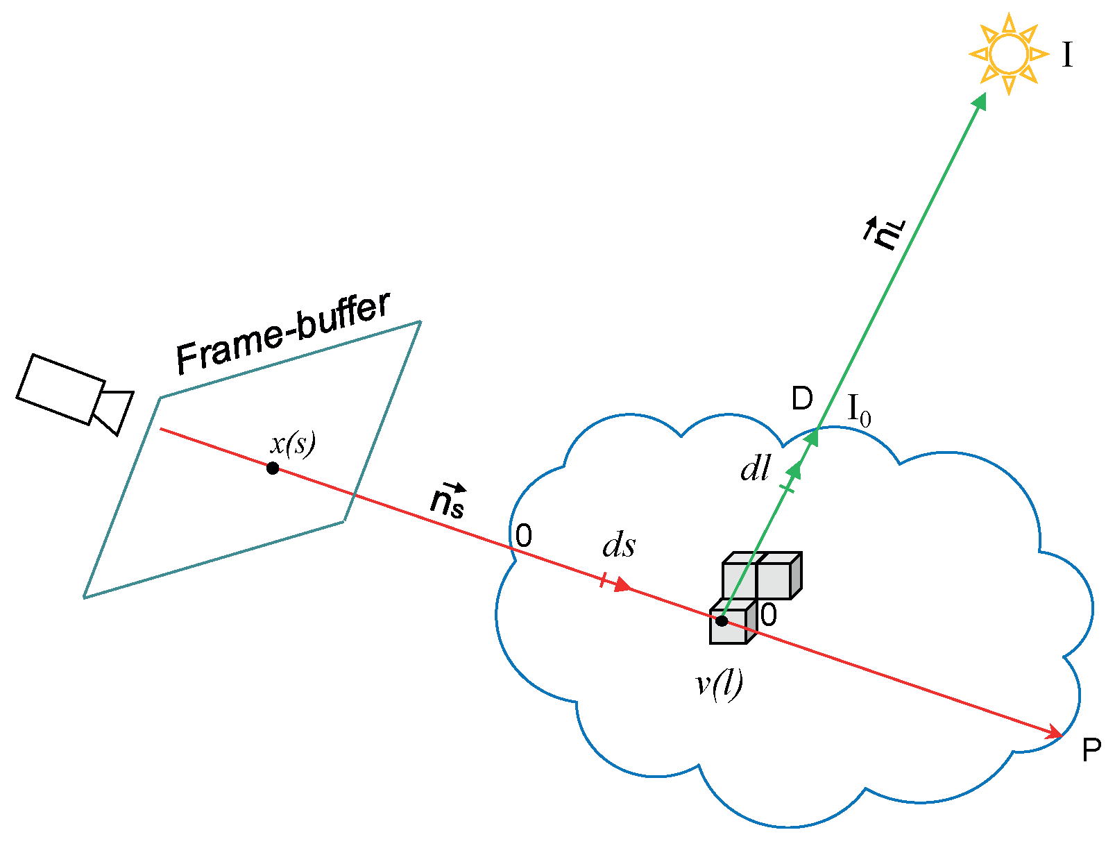
To perform cloud lighting and shading, our radiometry model uses a lightweight implementation based on the [34] equations with code optimisations to improve the performance and published in [35,36]. Accordingly, our proposed model is a hybrid method that balances the workload between the CPU and the GPU. As shown in Figure 2, the CPU or the GPGPU pre-calculates the light inside the cloud using voxels and considers light transmittance and scattering, as expressed in Equation  (1).

$$L\left(v\right)=\underset{\mathrm{absorption}}{\underbrace{I_o·T(0,D)}}+\underset{\mathrm{scattering}}{\underbrace{{\int }_0^{D}C\left(l\right)·T(0,l)dl}}$$

(1)

Let $L\left(v\right)$ be the light collected at point v inside the cloud; the first term represents the light reaching a given voxel containing v. For this term, $I_0$ represents the light intensity reaching the surface of the cloud, and T represents the transmittance of the cloud in the interval (0, D). D is the upper limit for the integral (cloud’s outer edge). The second term corresponds to the light scattered at every point along the ray collected in the voxel and accounts for the attenuation inside the cloud. Mathematically, we can calculate the scattering term as an integral of the approximation of the forward light scattering density function (C) multiplied by T in the interval (0, D).

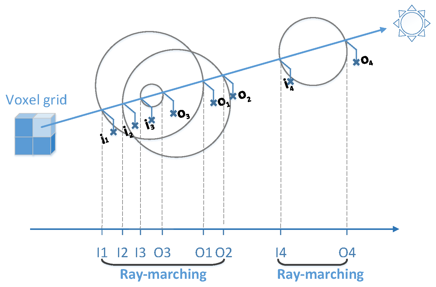
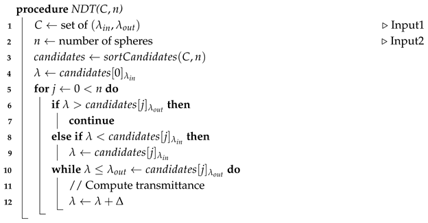
The shading pre-calculation phase uses the no-duplicate-tracing algorithm (NDT) in Equation (1) to avoid retracing in cases of sphere overlaps and inclusions, increasing the speed, as explained in [23,33]. Thus, as stated in Equation (2), let variables $(a,b,c)\in {\mathbb{R}}^3$ vector space, $(a_0,b_0,c_0)\in {\mathbb{R}}^3$ be the line origin coordinates and $\left(\overrightarrow{v_a},\overrightarrow{v_b},\overrightarrow{v_c}\right)\in {\mathbb{R}}^3$ be the direction vector. The $\lambda$ values include the ray-sphere collision input (${\lambda }_{in}$) and the ray-sphere collision output (${\lambda }_{out}$) of this straight-line equation (the $\lambda$ values represent the step size in the Euclidean straight-line parametric Equation (2)).

$$R\equiv \left\{\begin{array}{c}a=a_0+\lambda \overrightarrow{v_a}\hfill \\ b=b_0+\lambda \overrightarrow{v_b}\hfill \\ c=c_0+\lambda \overrightarrow{v_c}\hfill \end{array}\right.$$

(2)

Algorithm 1 and Figure 3 illustrate the NDT method. The sortCandidates(C,n) function sorts by ${\lambda }_{in}$ from nearest to farthest, inspired by the Insertion Sort algorithm [37], and Argument C is the set of lambdas from the parametric equation of the line colliding with n spheres under the pre-calculation phase ray. Furthermore, if the GPGPU is used for this algorithm, it spawns one thread per voxel by using the Compute Unified Device Architecture (CUDA), thus achieving a very high calculation speed.

Algorithm 1: No-Duplicate-Tracing.

On the other hand, the GPU calculates the projection on the frame buffer, accounting for the cloud transparency and light emitted from the cloud (scattering), as shown in Equation (3). Let $I\left(x\right)$ be the intensity of light at point x at the surface of the cloud:

$$I\left(x\right)={\int }_0^P\left[\underset{\mathrm{reflection}}{\underbrace{L\left(s\right)\tau \left(s\right)}}+\underset{\mathrm{scattering}}{\underbrace{L\left(s\right)\tau \left(s\right)P(\overrightarrow{n_s},\overrightarrow{n_l})}}\right]·T(0,s)ds$$

(3)

The first term represents the light from each voxel along the ray reflected in the gas volume according to its density, and $\tau$ is the light extinction coefficient. The second term represents the light from each voxel along the ray scattered according to the gas density and the Henyey–Greenstein [38] phase function (P) collected in the forward direction. Both terms are affected by attenuation from each point to the camera.

Note that Equation (1) is used to compute the light intensity reaching a given point (a voxel) inside the cloud, whereas Equation (3) is used to compute the light intensity exiting the cloud towards the observer. Equation (1) is precomputed either in the CPU or the GPGPU (CUDA) using the NDT algorithm, and the voxel values are stored for use in Equation (3), which is computed in the GPU. These equations have a positive impact on the overall system performance for entry-level computers. The NDT algorithm has been tested in MATLAB 14 with a wide range of test cases; however, it has not been formally proved.

Regarding the cloud shape, we decided to generate clouds by using a set of primitives called pseudo-spheroids, which modulate the radius of spheres via a randomised component to produce the nonregular aspect of the cloud surface during the render phase. The utilisation of few spheres to create cumuliforms along with our Gaussian cloud shape generator are relevant features of our work, as explained in [8,33].

3.2. Baseline for Cloud Dynamics Knowledge Acquisition

For the cloud dynamics, a parallel CUDA version of the grid-based [39] real-time fluid dynamics for games was implemented with the novel addition of guide points to translate fluid movement to cloud movement without altering the overall realism, as mentioned in [8,23]. To address the stable fluid method, which is used to solve the Navier–Stokes equations in a computer graphics simulation, as described in [40], it requires an implicit linear system solver such as, for example, the Jacobi, Gauss–Seidel or conjugate gradient methods. The motion of a viscous fluid is described by the Navier–Stokes equations, which are a set of partial differential equations that state the relation between pressure, velocity and forces during a specific period of time. As seen in Equation (4), the Navier–Stokes equations are based on Newton’s Second Law of Motion:

$$F=m·a$$

(4)

where m is the mass, a is the particle acceleration, and F is the resulting force.

There are other alternatives to describe fluid motion, such as the Euler equations used in [20]; however, the Navier–Stokes equations consider the viscosity of fluids as a property included in the equations. This property is needed when modelling cloud movement.

The governing equations for this work are the incompressible, unsteady Navier–Stokes equations with variable density and constant viscosity [41]. Equations used in the present work are based on those formulated in [39]:

$$\nabla ·\overrightarrow{u}=0$$

(5)

$${\displaystyle \frac{\partial \overrightarrow{u}}{\partial t}}=-(\overrightarrow{u}·\nabla )\overrightarrow{u}+\nu {\nabla }^2\overrightarrow{u}+\overrightarrow{F}$$

(6)

$${\displaystyle \frac{\partial \overrightarrow{\rho }}{\partial t}}=-(\overrightarrow{u}·\nabla )\overrightarrow{\rho }+k{\nabla }^2\overrightarrow{\rho }+\overrightarrow{S}$$

(7)

where $\overrightarrow{u}$ is the velocity vector field, $\nu$ is the kinematic viscosity of the fluid and $\overrightarrow{F}$ is the external force applied to the velocity field, $\overrightarrow{\rho }$ is the density vector field, k describes the density diffusion rate, $\overrightarrow{S}$ is the external force applied to the density field, and $\nabla =\left({\displaystyle \frac{\partial }{\partial x}},{\displaystyle \frac{\partial }{\partial y}},{\displaystyle \frac{\partial }{\partial z}}\right)$ represents the gradient. Equation (5) ensures mass conservation and initialises the velocity field to zero. Equation (6) represents the state of a fluid at a given instant in time, and it is modelled as a velocity vector field, so it is a function that assigns a velocity vector to every point in space. Equation (7) describes the mass conservation equation for a fluid with variable density. The idea behind considering a density function is to provide a realistic model of the visual textures in the game domain. Reading [39] for a more detailed explanation about this assumption is recommended. This work uses the [39] approach to simulate cloud motion, but the density Equation (7) is not required in this ontogenetic approach due to the use of the novel method of cloud guide point to translate the gaseous body according to the fluid grid velocity vectors, as explained in [23].

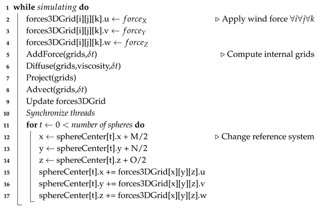
The basic Algorithm 2 based on the work of [39] has been modified in the following manner as cited in [8,23]:

Algorithm 2: Execution flow of the GPGPU parallel Navier–Stokes fluid solver simulator (CUDA).

Where the four consecutive states of the while loop are explained next:

• Add force: The process consists in adding a 3D force F (Equation (6)) to the velocity field in each cell of a 3D grid of dimensions (M,N,O) in the forces3DGrid[M][N][O] class attribute. For each grid cell, the new velocity will be:

  $$u=u_0+\delta t\times F.$$

  (8)

  where u is the velocity, $u_0$ is the previous value of u, $\delta t$ is the time increment and F is the applied force (wind).
• Diffusion: The diffusion is represented by the $\nu {\nabla }^2\overrightarrow{u}$ term in Equation (6), where the viscosity is the fluid internal resistance to flow. The resistance is caused by the diffusion of the momentum, such as velocity dissipation.
  As with advection, the diffusion can be approximated either with explicit or implicit methods, given a diffusion step.
  However, the explicit approach of diffusion is an explicit time-integration approach, and it is stated in [39] that it is unstable if the viscosity becomes large. As proof of this, ref.  [40] used this formulation and failed during the simulation.
  To overcome this limitation, the implicit version shown in Equation (9) is used:

  $$(I-\nu \delta t{\nabla }^2)u(x,t+\delta t)=u(x,t)$$

  (9)

  where I is the identity matrix. This equation remains stable for arbitrary time increments and viscosities and can be solved by iterative solvers such as Jacobi relaxation, Gauss–Seidel relaxation and the conjugate gradient. This work opts for the Jacobi approximation because the ontogenetic implementation does not require a lot of precision, so an efficient and reliable simulation is sufficient for standard industry purposes.
• Project: This routine forces the velocity to be mass conserving. The projection step amounts to solving a Poisson-type problem for the pressure variable to project the velocity into the space of divergence-free functions. This is an important property of real fluids which should be enforced. Visually it forces the flow to have many vortices which produce realistic swirly-like flows. It is therefore an important part of the solver as cited in [39,40].
• Advection: The advection function describes the transport of clouds, which is the resulting velocity of the fluid when moving.
  The advection can be calculated either with an explicit method such as the Euler method, a midpoint method such as Runge–Kutta or an implicit method such as [39,40].
  If an explicit method is used, Equation (10) results:

  $$r(t+\delta t)=r\left(t\right)+u\left(t\right)\delta t$$

  (10)

  where $r\left(t\right)$ is the particle position and $\delta t$ is the elapsed time while moving along the velocity field u. The problem is that when $u\left(t\right)\delta t$ is greater than the size of the grid cell, the simulation fails. Nevertheless, [8,23,39,40] overcomes this problem with an implicit solution approach as shown in Equation (11):

  $$q(x,t+\delta t)=q(x-u(x,t)\delta t,t)$$

  (11)

  where q is a quantity carried by the fluid, e.g., velocity, temperature or density.
  As cited in [40], “With stable fluid methods, the trajectory of the particle from each grid cell is traced back in time, to its former position. This approach is also referred as semi-Langrangian advection”.

At this point, we introduce the new approach of cloud motion using RNNs over each sphere parameter conforming the cumulus.

4. Proposed Method

In this work, we aim to replace the cloud dynamics method proposed by [8,23] with an RNN-based approach to improve the computational efficiency and address the limitations of the 3D spatial grid during real-time execution. In this method, a cloud is modelled on the basis of a set of spheres. Each sphere in the cloud is characterised by its position in three-dimensional space, given by the coordinates $(x,y,z)$, and its velocity vector, which is also in three dimensions $(vx,vy,vz)$. The velocities of the spheres are crucial, as they determine the future positions of the spheres and are thus the primary variables of interest in our study. The neural network’s objective is to predict the velocities of each sphere $(vx,vy,vz)$ at the next time step, given the current state of the system. This process includes the velocities of all spheres at the current time step. Working with velocities instead of coordinates allows us to obtain a method that is invariant to spatial translations. The rationale for using a neural network is that it facilitates the creation of a model that can learn complex interactions and dynamics from data, potentially capturing nonlinearities and dependencies that might be challenging to model explicitly. The motivation behind this configuration is to leverage machine learning to model and predict the complex dynamics of the cloud of spheres. By learning from simulation data generated by solving the Navier–Stokes equations, the neural network can potentially serve as a faster surrogate model, enabling rapid predictions without the need to solve the equations directly at each time step. In particular, the neural network learns and replaces the procedures presented in Lines 2 to 9 in Algorithm 2. To train the RNN, we used a spatial domain of 30 × 7 × 7 as the grid size in our learning prototype, and we applied the constants 0.4 for $\delta t$, 0.00001 for the atmosphere viscosity ($\nu$) and 0.2 for the wind force (F) as inputs. The wind force was set to a constant value and direction for all of the cells in the grid before starting the fluid simulation, as explained in Algorithm 2.

The following subsections first explain how the dataset for training was produced, and then, the details regarding the RNN architecture are presented. Finally, the training and inference details are described.

4.1. Dataset

We built a cloud dynamics dataset by using the simulation provided for the fluid machine proposed by [8,23]. To this end, we carried out a series of manual executions and data extractions from the method mentioned above, randomly modifying key simulation parameters such as the wind force and the number of spheres, which define the cumulus form, for up to a total of 1100 different simulations. Each of these simulations was composed of a sequence of 1000 iterations. Then, we applied the sliding window method to those sequences, with a window size set to 10 (see Figure 4 and Figure 5). The window size was calculated using a random search hyperparameter procedure in the range of 1 to 50 steps. Metrics associated with training (accuracy, etc.), and also execution times, were used as criteria for selecting the sliding window size parameter. The best value obtained which fulfils both criteria is a size value of 10. In the case of other cloud structures, the generalisation of the method is immediate since it is a standard hyperparameter search technique that depends on the training data used, not on the cloud structure used. We considered that a larger window would confer greater stability and robustness to the prediction despite worsening the model’s initialisation and execution time. Therefore, as the execution time is a key point to consider, we limited this parameter to meet our expectations regarding computational efficiency.

After the sliding window method was applied, the resulting dataset consisted of 1,013,312 training samples and 120,000 test samples. Each sample consists of a sequence of length 10 (the window size), containing the velocities in the three axes of motion $(x,y,z)$ for each sphere at every time step and meaning that each instance in the dataset contains 105 attributes for each timestep. The maximum number of spheres used during data collection was 35, which resulted in 105 $(x,y,z)$ coordinate tuples, and samples with fewer spheres were zero-padded to maintain size consistency. The target to predict is the next iteration in every case. A visual scheme of these processes can be seen in Figure 4 and Figure 5. The rationale for using 35 spheres is that it has the advantage of generating most types of cumuli by changing the radii of the pseudo-spheres following our parametrised Gaussian density equation as explained in [8,33].

Neural networks use a fixed-size input equal to the number of neurons in the input layer for their operation. Therefore, the variability in the number of spheres that make up the cloud to be simulated creates an issue regarding this requirement. To solve this problem, the zero-padding technique was used on samples with fewer than 35 spheres, which was set to be the maximum. This technique consisted of filling necessary positions in the input vector with zeros while maintaining size consistency with the input layer, occupying the vacancies in the missing spheres up to a defined maximum number. A post-padding technique is used, filling with zeros at the end of every sequence (training sample) when needed. This technique ensures that contextual information at the end of the sequence is preserved in the neural network training and ensures that the initial state of the RNN is always be the same. In addition, padding is only used in the first 10 sequences and the last 10, which represents an impact of 20 sequences out of the 1,013,312 used for training. In other words, 0.002% of padding data is added, the effect of which is negligible in relation to the information contained in the training set. Therefore, the effect is practically null in the creation of the model, and therefore in the inference and the generated output.

4.2. Deep Neural Network Architecture

Notably, once the data are stored and processed, there are multiple ways to input them into the neural models. First, the selection of an architecture that best suits this specific scenario was conducted. In the present work, the problem arises from an iterative behaviour in which the desired output in each iteration should form a variable-length sequence, which must be as short or as long as desired. Furthermore, as in any dynamic process, the previous stages, which can be understood as a trajectory, provide the necessary information to infer the successive stages of the sequence being emulated. These elements are often problematic when working with feedforward neural networks, which require a fixed and non-phase input and output size. These problems are solved by using RNNs, whose architectures are specifically designed to process time-dependent data streams.

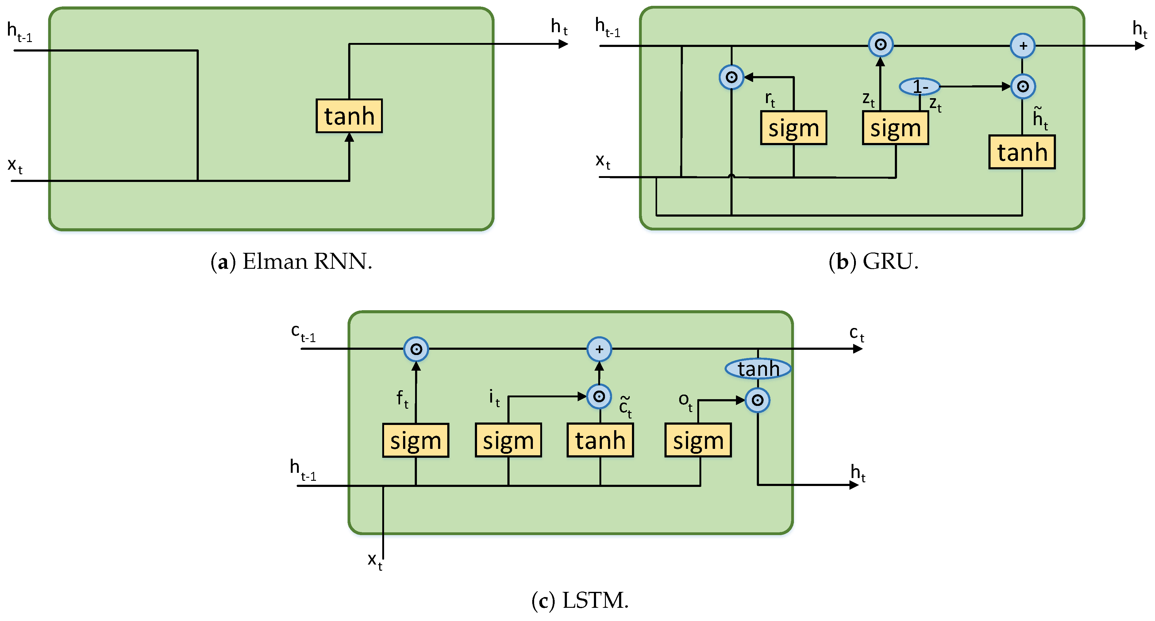
Within the family of recurrent neural networks, we found several types of recurrent units that perform this computation throughout time. Among the different units, the most important are the multi-layer Elman RNN [42], the Long Short-Term Memory (LSTM) [43] and the gated recurrent unit (GRU) [44], among others. An illustrative example of the working scheme of these models is presented in Figure 6 to provide a performance comparison:

• The Elman RNN [42] is one of the simplest RNN models, which means that it is fast; however, it has learning issues due to vanishing gradients. For each layer l of the network at timestep t, each hidden unit $h_t^l$ of that network computes the value shown in Equation (12).

  $$h_t^l=\tanh \left(x_t{W}_{ih}^T+b_{ih}+h_{t-1}^l{W}_{hh}^T+b_{hh}\right)$$

  (12)

  where $tanh$ is the hyperbolic tangent function, i.e., $tanh\left(x\right)={\displaystyle \frac{e^x-e^{-x}}{e^x+e^{-x}}}$; $x_t$ are the input data; $W_{ih}$ is the learnable weight matrix for the input data; $b_{ih}$ is the bias of the input data; $h_{t-1}^l$ is the output of the layer on the previous timestep; $W_{hh}$ is the learnable weight matrix for the output of the previous timestep; and $b_{hh}$ is the bias of the output of the previous timestep. Importantly, when $l>0$, $x_t$ is equal to $h_t^{l-1}$, i.e., the input is the output of the previous layer.
• LSTM is a more complex model designed to overcome the problem of vanishing and exploiting gradients, which is achieved by means of memory cells and gates that control the flow of information through the network [43]. However, this additional computation makes its learning slower than that of other alternatives. The three main components of the LSTM unit are as follows:
  • Memory cell $c_t$, which is responsible for storing long-term information.
  • Hidden state $h_t$, which represents the output of the LSTM on each timestep.
  • Gates that control the information flow. There are three gates: forget $f_t$, input $i_t$ and output $o_t$.
  For each layer of the LSTM, Equations (13)–(18) are computed for each unit:

  $$\begin{array}{cc}\hfill i_t& =\mathrm{sigmoid}\left(W_{ii}{x}_t+b_{ii}+W_{hi}{h}_{t-1}+b_{hi}\right)\hfill \end{array}$$

  (13)

  $$\begin{array}{cc}\hfill f_t& =\mathrm{sigmoid}\left(W_{if}{x}_t+b_{if}+W_{hf}{h}_{t-1}+b_{hf}\right)\hfill \end{array}$$

  (14)

  $$\begin{array}{cc}\hfill o_t& =\mathrm{sigmoid}\left(W_{io}{x}_t+b_{io}+W_{ho}{h}_{t-1}+b_{ho}\right)\hfill \end{array}$$

  (15)

  $$\begin{array}{cc}\hfill {\tilde{c}}_t& =\tanh \left(W_{ic}{x}_t+b_{ic}+W_{hc}{h}_{t-1}+b_{hc}\right)\hfill \end{array}$$

  (16)

  $$\begin{array}{cc}\hfill c_t& =f_t\odot c_{t-1}+i_t\odot {\tilde{c}}_t\hfill \end{array}$$

  (17)

  $$\begin{array}{cc}\hfill h_t& =o_t\odot \tanh \left(c_t\right)\hfill \end{array}$$

  (18)

  where $sigmoid\left(x\right)={\displaystyle \frac{1}{1+e^{-x}}}$ and $W_{i\mu }$ with $\mu \in \{i,f,o,c\}$ being the learnable weights of the input data for the input, forget and output gates and memory cell, respectively. $W_{h\mu }$ are the learnable weights for the hidden-to-hidden connection, $b_{i\mu }$ and $b_{h\mu }$ are the biases of these connections, and ⊙ represents the elementwise multiplication operation.
• Finally, the GRU is similar to LSTM in that it aims to maintain long-term information retention, avoiding vanishing and exploiting gradients while reducing the number of learnable parameters [44]. This objective is achieved by using only two gates: update $z_t$ and reset $r_t$, which control the amount of information that should be kept or forgotten, respectively. For each layer of the GRU, each unit computes the operations presented in Equations (19)–(22).

  $$\begin{array}{cc}\hfill r_t& =\mathrm{sigmoid}\left(W_{ir}{x}_t+b_{ir}+W_{hr}{h}_{t-1}+b_{hr}\right)\hfill \end{array}$$

  (19)

  $$\begin{array}{cc}\hfill z_t& =\mathrm{sigmoid}\left(W_{iz}{x}_t+b_{iz}+W_{hz}{h}_{t-1}+b_{hz}\right)\hfill \end{array}$$

  (20)

  $$\begin{array}{cc}\hfill {\tilde{h}}_t& =\tanh \left(W_{ih}{x}_t+b_{ih}+r_t\odot \left(W_{hh}{h}_{t-1}+b_{hh}\right)\right)\hfill \end{array}$$

  (21)

  $$\begin{array}{cc}\hfill h_t& =\left(1-z_t\right)\odot {\tilde{h}}_t+z_t\odot h_{t-1}\hfill \end{array}$$

  (22)

  where $W_{i\mu }$ with $\mu \in \{r,z,h\}$ represent the learnable weights for the input data for the reset and update gates and the output, respectively, and where $W_{h\mu }$ are the learnable weights for the hidden-to-hidden connection.

For this work, the proposed neural network architecture is as follows: an input layer followed by five stacked, hidden recurrent layers with 350 hidden units each and a final dense layer. The rationale behind this architecture is that the stacked RNN layers provide sufficient depth in the neural network to accurately learn the cloud dynamics. Additionally, each layer consists of 350 units, which is the maximum number of spheres multiplied by the number of timesteps; the idea is that each unit specialises in a specific axis of a sphere at a specific timestep. Finally, the output dense layer performs a linear transformation of the output of the last recurrent layer to produce the final output. This output is the velocity of each sphere of the cloud on the three axes of motion. For each layer, a dropout strategy is employed to avoid overfitting while training. We used a dropout value of 0.2, as it is the most recommended value for this learning approach. Importantly, the hidden units of the recurrent layers can be Elman, LSTM or GRU units, the selection of which is determined on the basis of the experimental study presented in Section 5. A schematic of the final RNN architecture is shown in Figure 7. The implementation was carried out by using the PyTorch 1.9 library for the Python 3.x programming language [45].

4.3. Training Details

The training process is specifically designed to teach the RNN to function as a surrogate for the traditional Navier–Stokes solver. The core objective is to minimize the discrepancy between the sphere velocities predicted by the network and the ground-truth velocities generated by the physics-based fluid simulation. To achieve this, we defined a clear training methodology, detailed as follows:

• Loss Function: We employed the Mean Squared Error (MSE) as the loss function between the predicted velocity values for each sphere on each axis of motion and the actual values, as shown in Figure 5 and defined in Equation (23):

  $$MSE(\widehat{V},V)={\displaystyle \frac{{\sum }_{i=1}^{N_s}{\sum }_{j=1}^3{({\widehat{v}}_{ij}-v_{ij})}^2}{3N_s}}$$

  (23)

  where $\widehat{V}=\{({\widehat{x}}_1,{\widehat{y}}_1,{\widehat{z}}_1),({\widehat{x}}_2,{\widehat{y}}_2,{\widehat{z}}_2),\dots ,({\widehat{x}}_{N_s},{\widehat{y}}_{N_s},{\widehat{z}}_{N_s})\}$ contains the predicted velocity values on each axis of motion for each sphere, $V=\{(x_1,y_1,z_1),(x_2,y_2,z_2),\dots ,(x_{N_s}$, $y_{N_s},z_{N_s}\left)\right\}$ is a vector that contains the actual velocity values on each axis of motion for each sphere, and ${\widehat{v}}_{ij}$ and $v_{ij}$ represent the coordinates $j\in \{x,y,z\}$ for the sphere i for the predicted values and the actual values, respectively. Finally, $N_s$ represents the number of spheres. This metric is ideal for this regression task as it quantifies the average squared difference between the predicted and actual velocity vectors, directly measuring the model’s prediction accuracy.
• Hyperparameter Tuning: The network’s architecture and training parameters were established through empirical evaluation to optimize performance. The final configuration consists of five stacked recurrent layers with 350 hidden units each, a dropout rate of 0.2 applied to each layer to mitigate overfitting, and a batch size of 64.
• Training Convergence: The model was trained using the ADAM optimizer [46] with ${\beta }_1=0.9$, ${\beta }_2=0.999$ for the exponential decay rates for the moment estimates and $ϵ={10}^{-8}$. These values are the default values recommended by the ADAM function in the PyTorch library. The initial learning rate value was set to ${10}^{-3}$, which was progressively reduced using an exponential decay scheduler, which was responsible for reducing this parameter as the training progressed, as expressed in Equation (24).

  $$l{r}_{t+1}=\gamma \left(l{r}_t\right)$$

  (24)
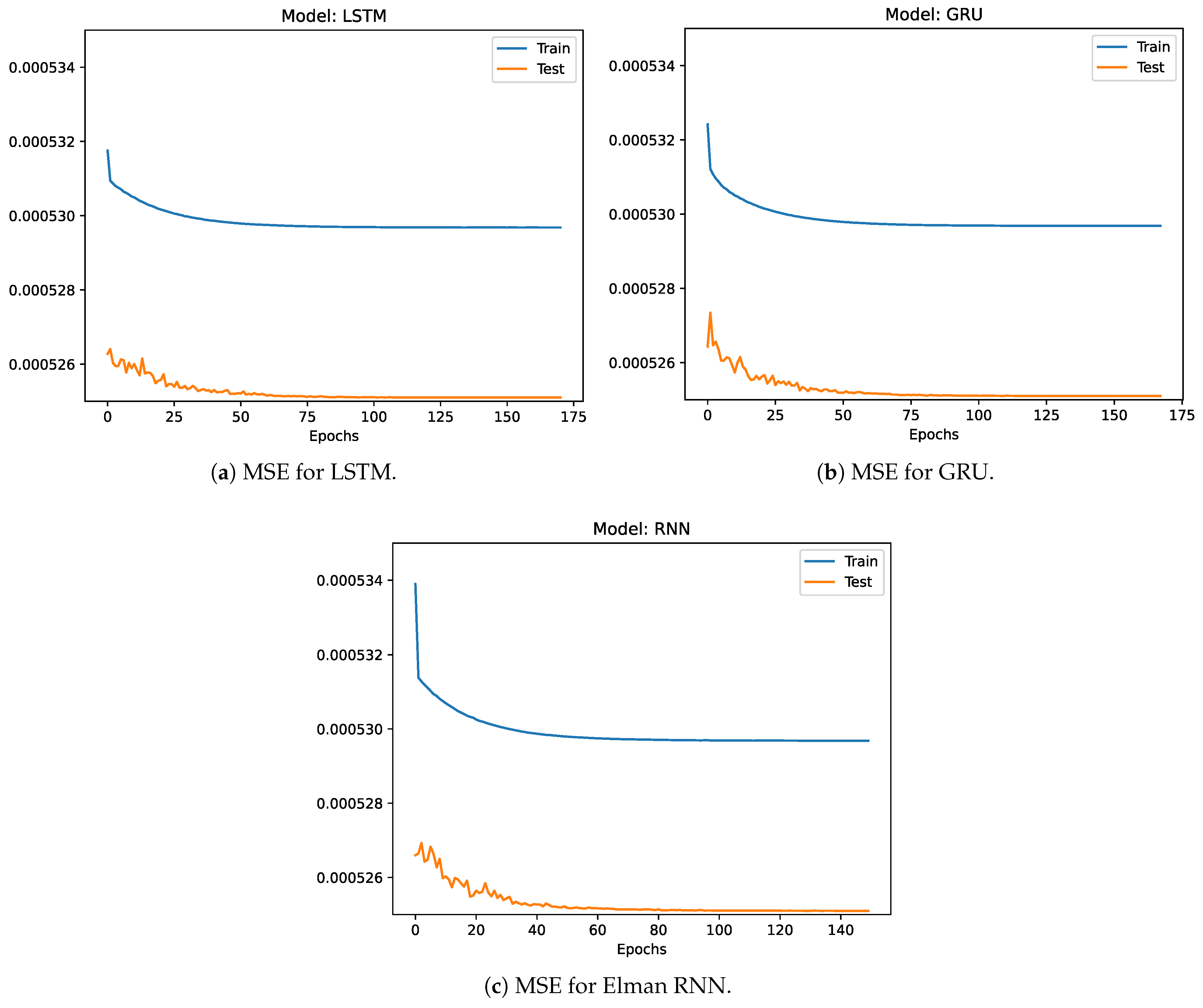
  For this particular case, we set the multiplicative factor of the learning rate decay ($\gamma$) to 0.95. This optimisation strategy aims to avoid overfitting. We monitored the MSE on a validation set to track convergence and prevent overfitting. As illustrated by the learning curves in Figure 8, the training process was concluded based on an early stopping policy, which terminated the training if the validation loss failed to show improvement over 20 consecutive epochs, i.e., the training did not improve over 10% of the total epochs.

The experiments were performed by using a laptop equipped with an Nvidia GeForce RTX 2060 (Turing, 1920 cores) running on a 64-bit Intel i7-Core CPU 10750H@2.60 GHz (10th generation, 2020) with 16 GB of random access memory (RAM).

Importantly, since this is a novel approach and the authors have not found any similar approach to that proposed in this paper, autoregressive integrated moving average (ARIMA) models [47] were developed to determine the velocity of each sphere in the three axes of motion, as they represent one of the most employed methods for time series forecasting. This method was employed as a baseline for comparing the performance of the proposed RNN method. The parameters employed on each individual ARIMA model for each variable were obtained by means of the auto.arima function of the forecast R package [48].

4.4. Inference Details

The inference process is the focus of the present work. At this point in the research, the neural network was tuned and ready to make predictions regarding cloud dynamics. This stage is directly related to the training phase since the inputs must have the same characteristics as those shown to the network during training. With this consideration in mind, the model was implemented in a function that initially receives ten iterations generated by the Navier–Stokes fluid solver. The network next accepts this input and generates, via prediction, the variation in the position of the spheres for the following time instant (see Figure 1). Then, in an iterative process, the network again accepts a sequence of size ten as input as formed by the newly predicted value and the previous nine. This process is repeated as many times as necessary.

4.5. Computational Complexity Analysis

To address the impact of the model’s components on its computational performance, we present a theoretical complexity analysis of the inference step, as execution time is a critical factor for real-time simulation. The computational complexity of a single inference step for a stacked RNN is primarily determined by the matrix multiplications within its recurrent layers. Actually, in this study, only the time complexity for the LSTM layer is addressed as it is the most complex model. Then, the complexity of the LSTM model is $O\left(4h\right(d+3+h\left)\right)$ [43] where h is the number of hidden units, and d is the dimension of input data, i.e., number of timesteps and number of features, which in this work is the number of spheres multiplied by 3.

As we are stacking multiple layers of this network, then the final computational complexity is:

$$O\left(L\right(4h(d+3+h)\left)\right)$$

(25)

where L is the number of stacked recurrent layers. The final linear layer adds a smaller term of $O(h·i)$. This formulation allows us to analyse the performance impact of each component:

• Window Size (d) and Number of Layers (L): The complexity scales linearly with both the window size and the number of layers. This means doubling the number of layers or the window size will roughly double the inference time. This justifies our choice of moderately sized values (10 for W and 5 for L) to maintain real-time performance.
• Number of Hidden Units (h): The complexity scales quadratically with the number of hidden units. This makes h the most critical hyperparameter for computational performance. Our choice of $h=350$ was empirically determined to provide sufficient model capacity without being prohibitively expensive.
• Type of Recurrent Unit: The choice between Elman RNN, GRU and LSTM primarily affects the constant factor hidden by the Big O notation. An LSTM unit involves more internal calculations (four gates) than a GRU (two gates and a candidate state) or an Elman RNN (one hidden state calculation). Consequently, for the same set of hyperparameters ($W,L,h,i$), an LSTM-based network is computationally more intensive than a GRU or Elman RNN. This presents a trade-off between the unit’s expressive power and its computational cost.
• Number of Spheres ($N_s$): The number of spheres directly influences the input feature size ($d=W\times N_s\times 3$). The complexity scales linearly with i. This theoretical result is strongly supported by our empirical findings in Section 5. As shown in Table 4 and Table 5, the mean inference time scales almost perfectly linearly with the number of cumuli (and thus, the total number of spheres) being simulated.

This analysis highlights the trade-offs made in designing the network and confirms that the number of hidden units (h) is the most sensitive parameter for performance, while the total number of spheres ($N_s$) results in a predictable, linear increase in computation time.

5. Experimental Results

As discussed in the introduction section, two objectives are associated with the proposal presented in this paper: (1) To obtain a nonlinear model by employing an RNN to replace the fluid dynamics model. The RNN works by means of the Navier–Stokes equations and has better quality in terms of the forecasting accuracy than traditional machine learning models (ARIMA). (2) More importantly, to prove that the execution of the inference is computationally more efficient.

The results are shown below and discussed in terms of these two objectives.

5.1. Metrics Evaluation

Table 3. Results of the metrics for the different methods used.

	Elman RNN	LSTM	GRU	ARIMA
Test MSE	0.000526	0.000525	0.000525	0.00815

shows the results corresponding to the mean of these errors for the ARIMA models and the different configurations of the trained recurrent networks, which included the Elman RNN, LSTM and GRU.

Figure 8 shows the evolution of the MSE value for the RNNs at the values considered for the training epochs. Both approaches, ARIMA and the deep neural networks, attempt to minimise the MSE between the target value and the predicted value, so it is an excellent metric for comparing these methods. As shown in Figure 8 and Table 3, the results obtained by the deep learning methods are relatively consistent, while the performance of ARIMA is significantly lower by an order of magnitude. Specifically, Figure 8 indicates that the networks learn without overfitting, as the training and test curves do not diverge. This result demonstrates that, regardless of the type of RNN unit used, a deep recurrent network can achieve results comparable to those of traditional models, aligning with the primary objective of this study.

5.2. Performance Evaluation

The performance of the proposed method was analysed in two experiments on two different types of computers, an older one and a newer one, to demonstrate the efficiency and linear progression of the computing time in relation to the number of cumuli and spheres. For this purpose, a multimedia project was implemented by using C++, OpenGL and the GLM math libraries for the host side and CUDA and the GLSL for the GPU side. The real-time RNN inference for cumuliform dynamics was implemented using PyTorch version 1.9 for C++ (libtorch). Due to the GPU utilisation in graphics rendering tasks, the CPU implemented the RNN inferences to balance the CPU/GPU load.

Importantly, the proposed RNN architecture produces small errors with respect to the fluid simulator. The output of the model is the inferred velocity distribution with a width other than zero. This width produces a long-term dispersion of the cloud on the X-axis when the number of iterations is big enough. Although this behavior is positive, we must keep its effect within a reasonable range, in order not to avoid premature cloud dispersal. In this sense, we introduce the parameter $\left(\delta \right)$. The width of this distribution is parameterised by a constant that we call the dispersion coefficient $\left(\delta \right)$, which can take any value between 0 and 1. The higher the value, the higher the dispersion of the cloud. The typical values for this coefficient are between 0 and 0.1 to avoid dispersion, with the value used in this case being 0.03. The position in $\widehat{x_i}$ for each sphere i is subsequently calculated via Equation (26), and thus, a reduction in the width of the distribution is achieved.

$${\widehat{x}}_i=\overline{X}+\delta (x_i-\overline{X})$$

(26)

where $\widehat{X}=\{\widehat{x_1},\widehat{x_2},\dots ,\widehat{x_{N_s}}\}$ is the set of all of the predicted x-coordinates for each sphere and $\overline{X}=mean\left(\widehat{X}\right)$.

5.2.1. First Experiment

Two sets of benchmarks were considered in the first experiment to evaluate the efficiency of our RNN method: one cumulus and ten cumuli with 35 spheres each. In each benchmark set, three algorithms for fluid dynamic simulation were analysed, including the RNN on a CPU (in particular, the LSTM was employed, as it produces the best results), CUDA with GPGPU optimisation and the multicore CPU algorithms described in [8,23] applied the maximum level for compiler speed optimisation.

The tests were performed at 1200 × 600 and 1920 × 1080 pixels in full high-definition (HD) with a ray marched landscape background, and samples were taken at nine different distances to the cloud centre. The first two benchmarks were performed by using an Nvidia GeForce GTX 1070 non-Ti (Pascal, 1920 cores) running on a 64-bit i-Core 7 CPU 860@2.80 GHz (first generation, 2009) with 12 GB of RAM.

As shown in Figure 9 (first benchmark), the RNN algorithm (our method) has a mean computing time of 16 to 17 ms irrespective of the distance and resolution (light blue and orange lines in the graph legend). In contrast, the CPU fluid dynamics algorithm (Algorithm 2) remains constant at more than 400 ms regardless of the distance and resolution (dark blue and green lines in the graph legend), while the CUDA fluid dynamics algorithm (Algorithm 2) varies from 80 to 241 ms depending on the distance and resolution (grey and yellow lines in the graph legend).

Figure 10 (second benchmark) shows the mean computation time measurements for ten cumuli when using the three fluid dynamics simulation modes and the two previously explained resolutions. The RNN mean execution time (our method, light blue and orange lines in the graph legend) varies between 149 ms and 166 ms depending on the distance at 1200 × 600 and 1920 × 1080 pixel resolution, respectively, while the CPU fluid dynamics algorithm (Algorithm 2, dark blue and green lines in the graph legend) maintains a constant execution time of approximately 450 ms at both resolutions. The execution time of the CUDA fluid dynamics algorithm (grey line in the graph legend) starts at 1302 ms at 1200 × 600 and then quickly decreases with distance, outperforming the fluid dynamics model on the CPU with Algorithm 2 (dark blue and green lines in the graph legend) at a distance of 10 and the RNN model (our method) at a distance of 35. At 1920 × 1080 pixels, the CUDA fluid dynamics algorithm is the slowest (yellow line in the graph legend).

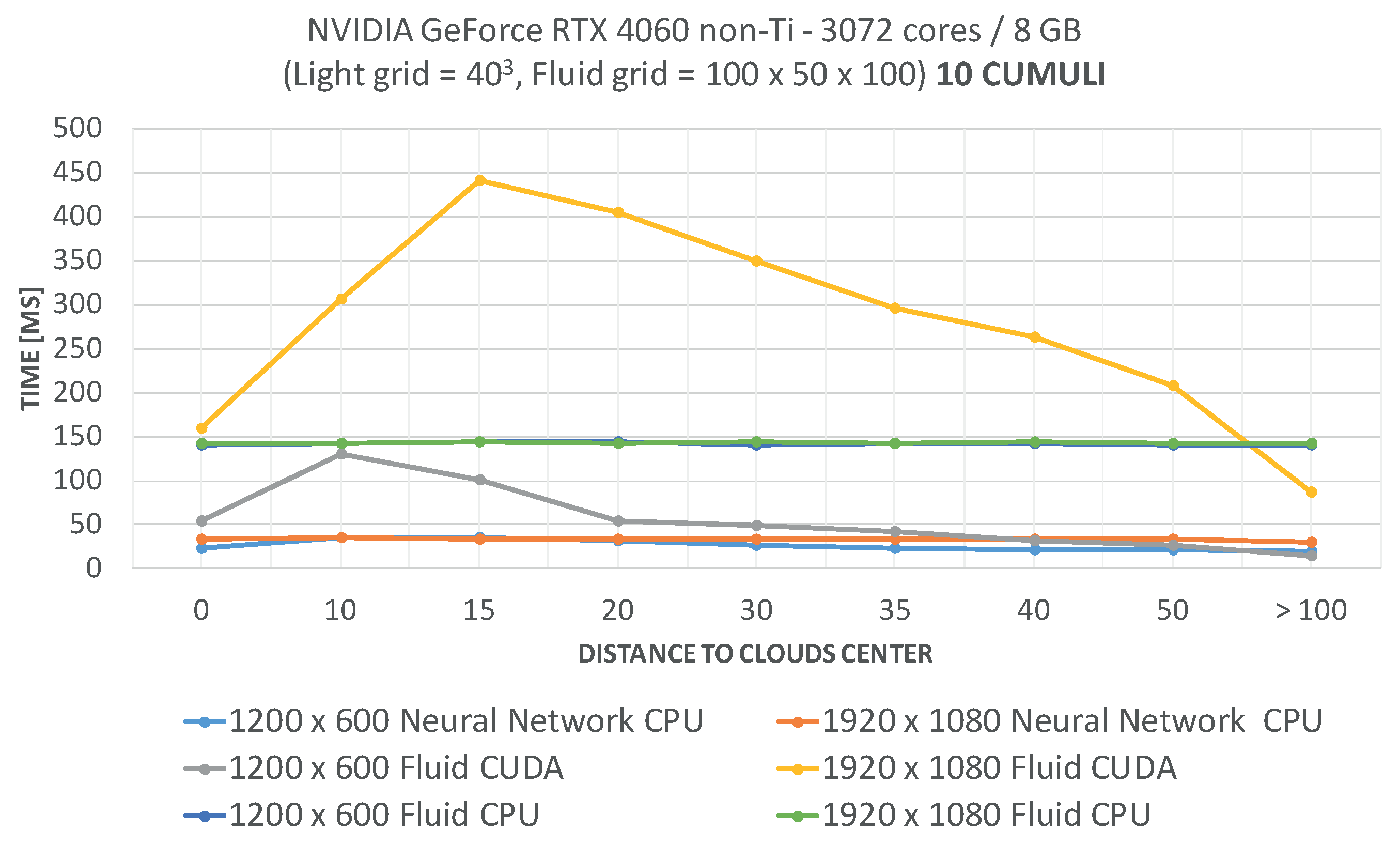
Additionally, a new benchmark was performed by using more recent hardware: an Nvidia GeForce RTX 4060 non-Ti (Ada Lovelace, 3072 cores) running on a 64-bit i-Core 7 CPU 14700K@5.6 GHz (14th generation, 2023) with 32 GB of RAM to render the ten-cumuli scene used for the previous benchmarks.

Figure 11 (third benchmark) shows the mean computing time for the three methods. As seen in the plots, the RNN method (light blue and orange lines in the legend) results in constant times between 26 ms and 33 ms for the tested resolutions. The CPU-based Navier–Stokes fluid solver (dark blue and green lines in the legend, Algorithm 2) has a constant mean computing time of 142 ms at both resolutions, which is four times slower than that of the RNN method. Furthermore, the CUDA-based Navier–Stokes fluid solver (Algorithm 2) is as fast as the RNN method at 1200 × 600 at medium and long distances from the cloud centre (grey line). However, at 1920 × 1080, this method can take up to 440 ms due to the graphical load (yellow line) and is the slowest.

5.2.2. Second Experiment

A second experiment was performed by using an Nvidia GeForce GTX 1070 (Pascal, 2048 cores) running on a 64-bit i-Core 7 CPU 8700@3.2 GHz laptop (8th generation, 2017) with 32 GB of RAM. The inferences were performed on the CPU instead of the GPU because much shorter times were obtained, as the GPU was busy rendering the clouds.

Table 4 shows the inference times in milliseconds for tests with different numbers of clouds and spheres in each cloud and different screen resolutions. Measurements were taken by displaying the rendering window and minimising it; in the latter case, the rendering process was not executed and therefore did not affect the inference times. These statistics were calculated using a sample of size 500 in each case.

When the rendering window is hidden, the differences between the measurements of central tendency at different resolutions are not significant and can be attributed to the state of the computer in each test, and the measurements of the central tendency scale almost linearly with the number of clouds. Furthermore, the standard deviations are small compared with their respective means, so it can be concluded that the data dispersion is not significant. In addition, for each test, the measurements of the central tendency are similar, and data asymmetry is not relevant; however, some outliers appear. The number of spheres seems to slightly increase the values of the central tendency.

Table 4. Inference time statistics in milliseconds for different resolutions, 1200 × 600 (medium) and 1920 × 1080 (Full HD). The render column refers to whether the render window was visible or not; when it was not visible the rendering process was not executed and therefore did not affect the inference times. The next column headings indicate the number of cumuli and spheres in each cumulus, respectively.

Resolution	Statistic	Render	1–35	5–35	10–35	1–60	5–60	10–60
Medium	Mean	yes	6.21	19.03	33.45	5.46	23.80	44.60
		no	2.64	13.09	25.11	2.70	16.26	30.69
	Median	yes	6.11	17.90	31.98	4.71	22.78	43.30
		no	2.45	12.29	24.21	2.52	12.88	24.65
	Std. dev.	yes	6.04	3.96	7.09	1.18	5.40	13.85
		no	0.51	2.38	3.34	0.50	4.10	7.65
Full HD	Mean	yes	9.76	36,34	55.11	8,70	38.82	63.12
		no	2.60	12.68	24.91	3.50	13.70	25.96
	Median	yes	8.92	34.63	41.74	8.40	43.57	48.25
		no	2.45	12.56	24.10	4.00	12.59	24.42
	Std. dev.	yes	2.56	15.19	27.73	1.84	14.32	30.25
		no	0.50	0.77	3.33	0.81	2.83	4.13

Table 4. Inference time statistics in milliseconds for different resolutions, 1200 × 600 (medium) and 1920 × 1080 (Full HD). The render column refers to whether the render window was visible or not; when it was not visible the rendering process was not executed and therefore did not affect the inference times. The next column headings indicate the number of cumuli and spheres in each cumulus, respectively.

Resolution	Statistic	Render	1–35	5–35	10–35	1–60	5–60	10–60
Medium	Mean	yes	6.21	19.03	33.45	5.46	23.80	44.60
		no	2.64	13.09	25.11	2.70	16.26	30.69
	Median	yes	6.11	17.90	31.98	4.71	22.78	43.30
		no	2.45	12.29	24.21	2.52	12.88	24.65
	Std. dev.	yes	6.04	3.96	7.09	1.18	5.40	13.85
		no	0.51	2.38	3.34	0.50	4.10	7.65
Full HD	Mean	yes	9.76	36,34	55.11	8,70	38.82	63.12
		no	2.60	12.68	24.91	3.50	13.70	25.96
	Median	yes	8.92	34.63	41.74	8.40	43.57	48.25
		no	2.45	12.56	24.10	4.00	12.59	24.42
	Std. dev.	yes	2.56	15.19	27.73	1.84	14.32	30.25
		no	0.50	0.77	3.33	0.81	2.83	4.13

When the rendering window is shown, the differences between the measurements of the central tendency at different resolutions seem to be significant. The measurements of the central tendency scale approximately linearly with the number of clouds but by a smaller factor than that in the hidden case. Furthermore, the standard deviations are not small compared with their respective means, and they are much larger than those in the hidden case. The number of spheres increases the values of the central tendency by a greater factor than that in the hidden case. In addition, the measurements of the central tendency are greater than those in the hidden case, especially if the screen resolution increases. We can conclude that when rendering is in progress, data transfer between the CPU and GPU significantly affects the inference times.

Table 5 compares the inference times on the same computer for a large-scale simulation at two resolutions for 84 and 167 cumuli with the dataset of 60 spheres each, producing a benchmark with 5040 and 10,020 spheres, respectively. However, if larger cumuli are needed, the most efficient approach is increasing the radii of the spheres with an average of 35 per cumulus or the parameters of the Gaussian shape generator, instead of using a larger number of spheres.

Table 5. Inference time statistics in milliseconds for large-scale simulation at 1200 × 600 (medium) and 1920 × 1080 (Full HD) resolutions. The fourth and fifth columns headings indicate the number of cumuli multiplied by 60 spheres, which result in 5040 and 10,020 spheres, respectively, for each benchmark.

Resolution	Statistic	Render	84–60 (≃5000)	167–60 (≃10,000)
Medium	Mean	yes	226.30	433.70
		no	220.35	433.61
	Median	yes	221.69	431.06
		no	219.92	426.84
	Std. dev.	yes	12.80	16.44
		no	6.76	19.56
Full HD	Mean	yes	225.71	441.63
		no	218.50	435.19
	Median	yes	224.82	436.72
		no	214.36	435.84
	Std. dev.	yes	7.79	20.16
		no	11.33	4.95

Table 5. Inference time statistics in milliseconds for large-scale simulation at 1200 × 600 (medium) and 1920 × 1080 (Full HD) resolutions. The fourth and fifth columns headings indicate the number of cumuli multiplied by 60 spheres, which result in 5040 and 10,020 spheres, respectively, for each benchmark.

Resolution	Statistic	Render	84–60 (≃5000)	167–60 (≃10,000)
Medium	Mean	yes	226.30	433.70
		no	220.35	433.61
	Median	yes	221.69	431.06
		no	219.92	426.84
	Std. dev.	yes	12.80	16.44
		no	6.76	19.56
Full HD	Mean	yes	225.71	441.63
		no	218.50	435.19
	Median	yes	224.82	436.72
		no	214.36	435.84
	Std. dev.	yes	7.79	20.16
		no	11.33	4.95

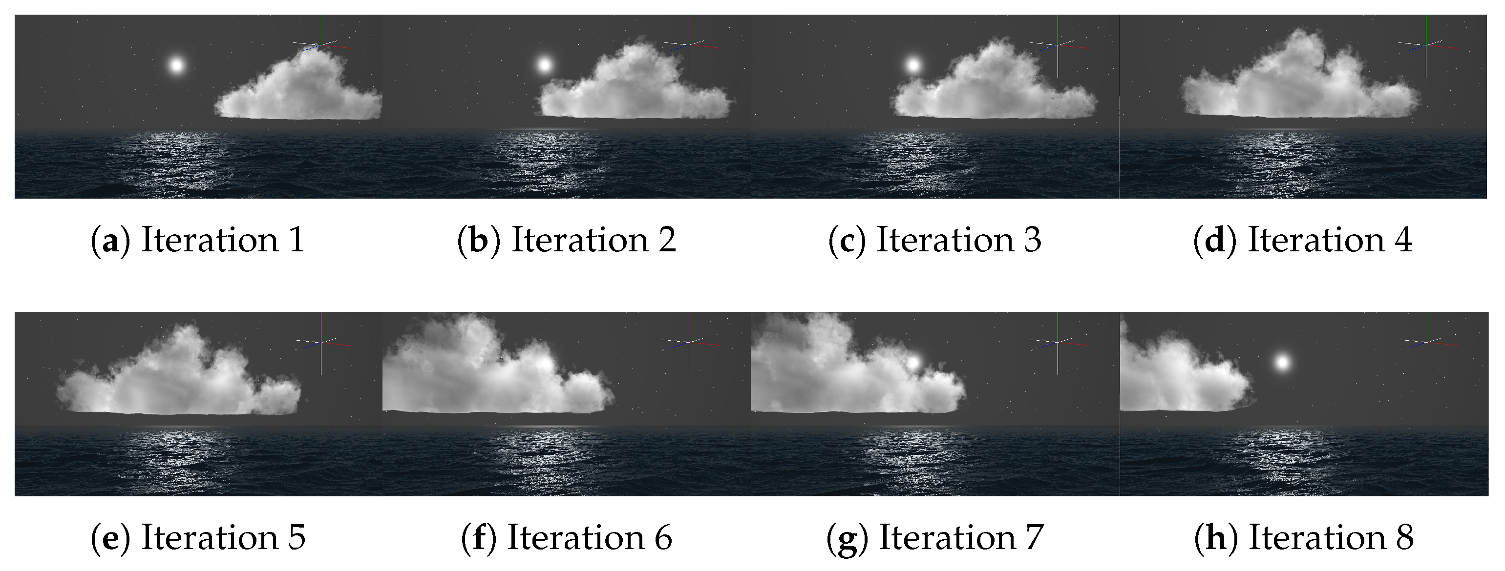
To appreciate the natural likelihood of the visual rendering of cumulus atmospheric dynamic simulation, Figure 12 and Figure 13 illustrate a sequence of eight instants of a cumulus movement by using our trained RNN for fluid dynamics for 35 and 60 spheres, respectively. The cumulus correctly evolves according to the wind advection force vectors during RNN knowledge acquisition, dragging the pseudospheres and producing rich forms across the space with RNN inferences.

On the other hand, Figure 14 shows eight iterations depicting the evolution of strati that rely on solving exact thermodynamics/fluids equations as documented in [26].

6. Discussion and Limitations

The advantage of our method over the CUDA fluid dynamic simulation method, which is based on the work of [8,21,39], is its ability to emulate cloud movement with constant performance regardless of the size of the three-dimensional grid. Thus, the clouds can be animated over an infinite scenario without computational spatial bounds or other data structures requiring memory. The ability to conform our cumuli by using pseudospheres or pseudo-ellipsoids as shown in [49,50,51], along with the RNN, is another feature that enables fine control over the cumuliform gaseous resemblance that other real-time methods based on meteorological datasets or meshes lack [9]. Furthermore, the sphere positions were useful as weights for our RNN input during training and inference.

In our tests, we improved the average computation time for each time step of the simulation in [32] from 0.031 s on an Nvidia Titan X GPU to 0.016 s on a GTX 1070 non-Ti (first experiment) and 0.006 s on a GTX 1070 laptop (second experiment) for the same number of cumuli. We also outperformed the best case in [26], which used an Nvidia GTX 1080 with a $128\times 48\times 128$ grid size employing 0.040 s per frame. With respect to the work in [31], which used a 4 GHz CPU and an Nvidia RTX 2060 GPU (+11% faster in effective speed than an Nvidia GTX 1070 (https://gpu.userbenchmark.com/Compare/Nvidia-RTX-2060-vs-Nvidia-GTX-1070/4034vs3609, accessed on 22 August 2025 with $1280\times 720$ pixel screen resolution), we obtained very similar real-time performances and better cumuliform rendering quality even when using older equipment with higher screen resolutions.

The previous comparison is qualitative because the source code of the mentioned work is not publicly available, so no objective measurement could be made. While the Goswami rendering method is more efficient than our method in terms of transforming the cloud maps into a unique 3D hypertexture, we achieve quite a similar performance in terms of arranging a set of spheres as cloud primitives in the scene bounding box. The Goswami inference method is based on Deep Convolutional Generative Adversarial Neural Networks (DCGANs), which were trained to generate synthetic images. Goswami then employed this technique to create a cloud image for each frame without considering the dynamics of cloud movement in the neural network. These dynamics were incorporated into the input parameters for the inference made in the DCGAN to generate a sequence of cloud images. Therefore, the DCGAN does not model the dynamics of cloud movement but rather specific image sequences that it has learned from the input sequences. According to the authors, these sequences are very limited in number, as there are 13 videos. From the previous description, it becomes evident that the proposed models are very different, and the structures of the neural network models are not comparable. However, they can be compared by using the time metrics associated with the computational generation of the models and the image sequences. As a general rule, DCGANs are more complex to train than RNNs are, and in fact, the authors indicate that they required 2000 to 3000 epochs to train the two networks used, which they call T_DCGAN and R_DCGAN, and each training epoch ranged between 6.52 and 9.07 s depending on the encoding, grayscale, and RGB used for the images obtained from the video sequences. According to the authors, these images have a resolution of 256 × 256 pixels; this resolution is inadequate for simulations that render reasonable image quality. In the case of the model proposed in this paper, approximately 200 epochs were used for network training. However, the training times of each epoch were greater since the amount of data considered was much greater than that by Goswami, as described in Section 4.1. This divergence again indicates that the models are different due to the datasets used in each neural network type.

With respect to the inference times of the networks for image generation, Goswami indicates that “The total per-frame execution time of the proposed method is an average of 3.02 ms”. In the case of the RNN described in this paper, the average result is 2.60 ms per inference step for Full HD (1920 × 1080) resolution qualities without landscape rendering. This advantage is shown in

Table 6. Comparison of the current state-of-the-art real-time cloud dynamics simulation works.

Author	Advantages	Disadvantages	Best-Case Time
[32]	Cloud initial conditions generation	Low realism	31 ms
		Expensive hardware
[26]	Very high realism	3D grid constraints	40 ms
	Use of real fluid/thermodynamics equations	Cumuli look like smoke
		Lacks cumulus long space transition
[31]	Straightforward knowledge acquisition	Lacks cumulus long space transition	3.02 ms
	Physical equations not required
Ours	3D lattice not required	Training of the cloud spheres set required	2.60 ms
	Physical equations not required
	Expensive hardware not required

in bold text, where we obtain 2.60 ms as the best-case time based on the benchmarks reported in Table 4 in bold text.

Additionally, our method reduces the simulation time step compared with previous methods, e.g., [21]. A comparison of the current state-of-the-art studies is detailed in Table 6.

To evaluate the overall system performance on a standard computer in frames per second (FPS), we used the same equipment for the first experiment in Section 5.2.1. The resulting measurement exceeds the minimum required real-time threshold in most cases.

Table 7. Frames per second statistics in the proposed method for different screen resolutions, 1200 × 600 (medium) and 1920 × 1080 (Full HD) at three distances from the observer’s view point. The last two columns headings indicate the number of cumuli and spheres per cumulus, respectively. Each cumulus is conformed with 35 pseudo-spheres of size 2.9 units, mean ${\mu }_x=0, {\mu }_y=0, {\mu }_z=0$ and standard deviation ${\sigma }_x=3.8 ,{\sigma }_y=1.7 ,{\sigma }_z=3.7$. See [33].

Resolution	Distance	1–35 (FPS)	10–35 (FPS)
	Near	55	34
Medium	Mid-distance	74	33
	Far	114	45
	Near	16	10
Full HD	Mid-distance	34	18
	Far	98	30

depicts the FPS for medium and Full-HD screen resolutions for one and ten cumuli, respectively, with 35 spheres each.

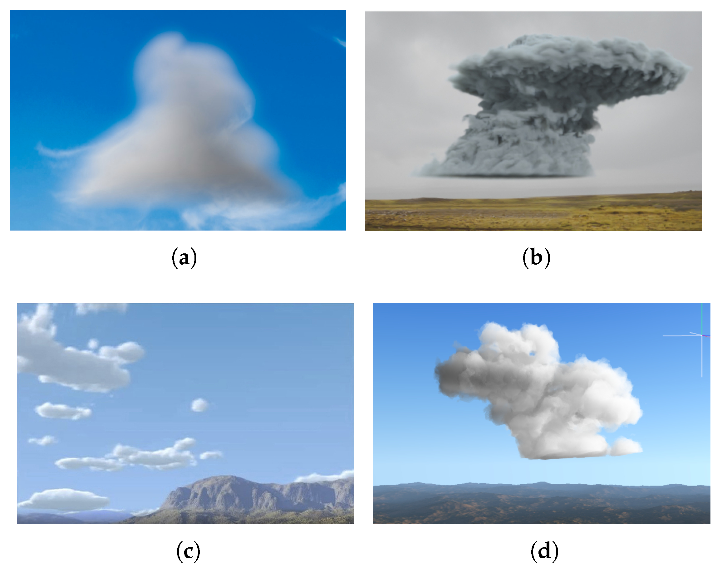
The visual quality of cumuli rendering by our method must sustain the optimum real-time performance above 30 FPS while running the fluid dynamics RNN inference within the required time in most cases. The use of pseudo-spheroidal primitives to cause the clouds to conform has many advantages for AI but imposes constraints on the time complexity and the calculations performed by the rendering shader algorithm. However, the visual quality of our rendering method outperforms a significant number of previous and present related methods. The likelihood of the resulting clouds can be evaluated empirically in the comparison between our rendering method (Figure 15a) and a real photograph (Figure 15b). To validate the realism, we applied the quantitative metric of the Universal Quality Image Index (UQI) method by [52], obtaining a correlation score of 0.89 with the aforementioned images, 1 being high quality.

For further comparison between our method and the referenced state-of-the-art real-time cloud dynamics works, we include snapshots of these clouds in Figure 16.

According to the results shown in Figure 9, Figure 10 and Figure 11, our method can be applied in computer games, flight simulation systems, atmospheric simulations, educational tools for climate awareness, etc., without losing performance. This goal is possible because of the better efficiency of the RNN when compared to other types of fluid simulation techniques. Furthermore, this method can be applied in the computer game industry when rendering outdoor scenarios with medium screen resolutions to improve both the computing efficiency and the user experience. The realism and likelihood of cumulus atmospheric behaviour are sufficiently accurate, along with various forms that the RNN randomises, avoiding expensive computational overhead at resolutions lower than 1920 × 1080. Higher realism in terms of aspects such as rendering quality implies a severe reduction in the overall real-time performance that would affect users with basic hardware.

It is important to keep in mind that outputs produced by neural networks are approximations of the real solution to the problem. Even if we use a very large sample and greatly reduce the error between the predicted value and the real value, there may always be traces of this approximation. Notably, the data used to train the network were derived from the results calculated by the solver of the incompressible NSE, and these results are already approximations of the mathematical solutions to the equations. Therefore, the solution provided by the neural network will always be an approximation with very high accuracy regarding the calculated data from the NSE, but it will never have better accuracy than the solution to the original incompressible NSE. However, the accuracy of the neural network can be tuned to obtain a more precise model. As the accuracy approaches 100%, the model more closely reproduces the output of the original equation solver presented in Algorithm 2. Therefore, under our iterative method, where the previously predicted values are used to predict the next values, these small errors can be expected to propagate and increase as the number of time steps increases. The use of neural networks also involves an additional problem: the dependence of their performance on the training data used. Therefore, proper performance requires training with the correct data. For the same reason, when scaling the method to a larger number of spheres and thus creating a new network that can handle this increased size, the network parameters must be retrained. This retraining action should not be a problem in terms of the method’s performance, as by following the same training process, the new network should converge back to the correct operation. However, this process can be tedious when the problem requires a very long training time.

7. Conclusions and Future Work

This paper presents a new real-time realistic method for simulating cumuliform fluid dynamics with RNNs. By using a GPU pseudosphere-based approach, we achieve natural-looking movement of cumuli with a diversity of forms after RNN deep learning. Additionally, we achieve better overall system efficiency at resolutions lower than 1920 × 1080 and overcome the need for spatial grid bounds due to the use of an RNN trained with the result of the atmospheric physical simulation previously executed in parallel on the GPGPU. The proposed method consists of training different types of RNNs, such as LSTM, the GRU or the Elman RNN, to iteratively obtain a cloud dynamics predictor, similar to a multidimensional time series forecasting problem. Therefore, the neural model solves the fluid physics equations normally calculated by the software engine more efficiently during real-time execution. The empirical results demonstrate a constant and high real-time performance, which implies the low energy consumption of our RNN method compared with other limited or computationally expensive fluid dynamics models. Furthermore, scalability is also a relevant advantage of our method since the complexity of the method increases linearly with the number of spheres. Thus, the training and implementation of a neural network capable of moving an arbitrary number of spheres are straightforward when using this method, as shown in the two different experiments, which demonstrate that the proposed method achieves a much better computational efficiency than that of the alternatives proposed in the literature. Under these premises, we can confirm the initial hypothesis and the valuable application of our algorithm in computer simulations of natural phenomena.

In addition, this work may open the door to exploring these advantages in other similar processes in which computational efficiency is a crucial issue and in which some loss of precision in the simulation results of the model is acceptable. We refer here to the context of simulation tools for which the dynamics of the bodies involved constitute a computationally complex process; this method could be applied in the same way to reduce the computational time in those contexts. Additionally, the method can be used to obtain neural network approximation functions for more comprehensive models that can incorporate features such as water vapour, cloud density, phase transitions, and buoyancy while maintaining the computational efficiency necessary for integration in realistic scenarios such as those presented in the paper. Regarding future activities, we intend to work on the correlation between these characteristics and data based on the associated physical model simulations. To incorporate these new physical parameters, new equations of state must be added to the solver. For example, in the case of temperature, pressure, and cloud density in [53], a new equation of state is added that allows these three characteristics to be correlated with the fluid model. For each set of characteristics, a state equation can therefore be added to the Navier–Stokes fluid solver. The data generation procedure for training will use this new solver, modified by adding the state equations.

Under the current assumption, if a different LSTM model is run to control each cloud present in the simulation, the execution time increases linearly with the number of clouds since these models are executed sequentially. However, we believe that this method has the potential to support parallelisation of these processes on the GPU, thus achieving the minimum time regardless of the number of clouds.

On the other hand, in the present work, we have implemented an LSTM network configured to predict the motion of up to 60 spheres, intrinsically limited to this number by the architecture of this particular network. As mentioned above, this method has the advantage of being fully scalable by simply increasing the number of input neurons to the desired value, and thus, when trained with appropriate data, one can extend the results of the present method to clouds composed of an arbitrary number of spheres. In future work, we propose scaling the size, increasing the cloud diversity and experimentally corroborating that the computational efficiency is also maintained for this case. In addition, an exhaustive study of recurrent neural network types and associated metrics will be conducted. The objective will be to provide different types of networks (RNN, LSTM, GRU, and Transformers) as a selection framework based on these metrics, computational performance, and the realism of the images produced.

References

1. Chen, Y.; Yang, H. Numerical simulation and pattern characterization of nonlinear spatiotemporal dynamics on fractal surfaces for the whole-heart modeling applications. Eur. Phys. J. B 2016, 89, 181. [Google Scholar] [CrossRef]
2. Binder, K. Computer simulations of critical phenomena and phase behaviour of fluids. Mol. Phys. 2010, 108, 1797–1815. [Google Scholar] [CrossRef]
3. den Hoogen, J.V.; Meijer, S. Gaming and Simulation for Railway Innovation. Simul. Gaming 2015, 46, 489–511. [Google Scholar] [CrossRef]
4. Zamri, M.N.; Sunar, M.S. Atmospheric cloud modeling methods in computer graphics: A review, trends, taxonomy, and future directions. J. King Saud Univ.-Comput. Inf. Sci. 2020, 34, 3468–3488. [Google Scholar] [CrossRef]
5. Goswami, P. A survey of modeling, rendering and animation of clouds in computer graphics. Vis. Comput. 2021, 37, 1931–1948. [Google Scholar] [CrossRef]
6. Huang, B.; Chen, J.; Wan, W.; Bin, C.; Yao, J. Study and Implement About Rendering of Clouds in Flight Simulation. In Proceedings of the 2008 International Conference on Audio, Language and Image Processing, Shanghai, China, 7–9 July 2008; pp. 1250–1254. [Google Scholar] [CrossRef]
7. Yusov, E. Eurographics/ACM SIGGRAPH Symposium on High Performance Graphics. In Proceedings of the High-Performance Rendering of Realistic Cumulus Clouds Using Pre-Computed Lighting, Lyon, France, 23–25 June 2014; pp. 127–136. [Google Scholar] [CrossRef]
8. Jiménez de Parga, C. High-Perfomance Algorithms for Real-Time GPGPU Volumetric Cloud Rendering from an Enhanced Physical-Math Abstraction Approach. Ph.D. Thesis, National Distance Education University (UNED), Madrid, Spain, 2019. [Google Scholar] [CrossRef]
9. Bouthors, A. Realistic Rendering of Clouds in Real-Time. Ph.D. Thesis, Université Joseph Fourier, Grenoble, France, 2008. [Google Scholar]
10. Kallweit, S.; Müller, T.; Mcwilliams, B.; Gross, M.; Novák, J. Deep Scattering: Rendering Atmospheric Clouds with Radiance-Predicting Neural Networks. ACM Trans. Graph. 2017, 36, 231. [Google Scholar] [CrossRef]
11. Lye, K.; Mishra, S.; Ray, D. Deep learning observables in computational fluid dynamics. arXiv 2019, arXiv:1903.03040. [Google Scholar] [CrossRef]
12. Yu, C.; Bi, X.; Fan, Y. Deep learning for fluid velocity field estimation: A review. Ocean. Eng. 2023, 271, 113693. [Google Scholar] [CrossRef]
13. Li, Z.; Farimani, A.B. Graph neural network-accelerated Lagrangian fluid simulation. Comput. Graph. 2022, 103, 201–211. [Google Scholar] [CrossRef]
14. Lino, M.; Fotiadis, S.; Bharath, A.A.; Cantwell, C.D. Current and emerging deep-learning methods for the simulation of fluid dynamics. Proc. R. Soc. A 2023, 479, 20230058. [Google Scholar] [CrossRef]
15. Sun, L.; Gao, H.; Pan, S.; Wang, J.X. Surrogate modeling for fluid flows based on physics-constrained deep learning without simulation data. Comput. Methods Appl. Mech. Eng. 2020, 361, 112732. [Google Scholar] [CrossRef]
16. Zhu, Y.; Zabaras, N.; Koutsourelakis, P.S.; Perdikaris, P. Physics-constrained deep learning for high-dimensional surrogate modeling and uncertainty quantification without labeled data. J. Comput. Phys. 2019, 394, 56–81. [Google Scholar] [CrossRef]
17. Hassanian, R.; Riedel, M.; Bouhlali, L. The capability of recurrent neural networks to predict turbulence flow via spatiotemporal features. In Proceedings of the 2022 IEEE 10th Jubilee International Conference on Computational Cybernetics and Cyber-Medical Systems (ICCC), Reykjavík, Iceland, 6–9 July 2022; IEEE: Washington, DC, USA, 2022; pp. 335–338. [Google Scholar] [CrossRef]
18. Miyazaki, R.; Yoshida, S.; Dobashi, Y.; Nishita, T. A method for modeling clouds based on atmospheric fluid dynamics. In Proceedings of the Ninth Pacific Conference on Computer Graphics and Applications, Pacific Graphics 2001, Tokyo, Japan, 16–18 October 2001; pp. 363–372. [Google Scholar] [CrossRef]
19. Overby, D.; Melek, Z.; Keyser, J. Interactive physically-based cloud simulation. In Proceedings of the 10th Pacific Conference on Computer Graphics and Applications, 2002. Proceedings, Beijing, China, 9–11 October 2002; IEEE: Washington, DC, USA, 2002; pp. 469–470. [Google Scholar] [CrossRef]
20. Harris, M. Real-Time Cloud Simluation and Rendering. Ph.D. Thesis, Chapel Hill, Chapel Hill, NC, USA, 2003. [Google Scholar]
21. Dobashi, Y.; Kusumoto, K.; Nishita, T.; Yamamoto, T. Feedback Control of Cumuliform Cloud Formation Based on Computational Fluid Dynamics. ACM Trans. Graph. 2008, 27, 1–8. [Google Scholar] [CrossRef]
22. Guo, H.; Pang, J.; Shan, Z. Real-Time Dynamic Cloud Simulation Based on Multi-core and Multi-thread. In Proceedings of the 2012 Fourth International Conference on Multimedia Information Networking and Security, Nanjing, China, 2–4 November 2012; IEEE: Washington, DC, USA, 2012; pp. 241–245. [Google Scholar] [CrossRef]
23. Jiménez de Parga, C.; Gómez Palomo, S. Parallel Algorithms for Real-Time GPGPU Volumetric Cloud Dynamics and Morphing. J. Appl. Comput. Sci. Math. 2019, 13, 25–30. [Google Scholar] [CrossRef]
24. Goswami, P.; Neyret, F. Real-time landscape-size convective clouds simulation and rendering. In Proceedings of the VRIPHYS 2017-13th Workshop on Virtual Reality Interaction and Physical Simulation, San Francisco, CA, USA, 27 February–1 March 2015. [Google Scholar] [CrossRef]
25. Silva, A.R.; Silva, A.R.; Gouvêa, M.M. A novel model to simulate cloud dynamics with cellular automaton. Environ. Model. Softw. 2019, 122, 104537. [Google Scholar] [CrossRef]
26. Hädrich, T.; Makowski, M.; Pałubicki, W.; Banuti, D.T.; Pirk, S.; Michels, D.L. Stormscapes: Simulating cloud dynamics in the now. ACM Trans. Graph. (TOG) 2020, 39, 175. [Google Scholar] [CrossRef]
27. Mukina, K.; Bezgodov, A. The Method for Real-time Cloud Rendering. Proc. Procedia Comput. Sci. 2015, 66, 697–704. [Google Scholar] [CrossRef]
28. Roehrl, M.A.; Runkler, T.A.; Brandtstetter, V.; Tokic, M.; Obermayer, S. Modeling System Dynamics with Physics-Informed Neural Networks Based on Lagrangian Mechanics⁎⁎This work was sponsored by the German Federal Ministry of Education and Research (ID: 01 IS 18049 A). IFAC-PapersOnLine 2020, 53, 9195–9200. [Google Scholar] [CrossRef]
29. Faroughi, S.A.; Pawar, N.; Fernandes, C.; Das, S.; Kalantari, N.; Mahjour, S.K. Physics-Guided, Physics-Informed, and Physics-Encoded Neural Networks in Scientific Computing. arXiv 2022, arXiv:2211.07377. [Google Scholar] [CrossRef]
30. Lennon, K.R.; McKinley, G.; Swan, J. Scientific machine learning for modeling and simulating complex fluids. Proc. Natl. Acad. Sci. USA 2022, 120, e2304669120. [Google Scholar] [CrossRef]
31. Goswami, P.; Cheddad, A.; Junede, F.; Asp, S. Interactive landscape–scale cloud animation using DCGAN. Front. Comput. Sci. 2023, 5, 957920. [Google Scholar] [CrossRef]
32. Zhang, Z.; Ma, Y.; Li, Y.; Li, F.W.; Shum, H.P.; Yang, B.; Guo, J.; Liang, X. Cumuliform cloud formation control using parameter-predicting convolutional neural network. Graph. Model. 2020, 111, 101083. [Google Scholar] [CrossRef]
33. Jiménez de Parga, C.; Gómez Palomo, S. Efficient Algorithms for Real-Time GPU Volumetric Cloud Rendering with Enhanced Geometry. Symmetry 2018, 10, 125. [Google Scholar] [CrossRef]
34. Max, N. Optical Models for Direct Volume Rendering. IEEE Trans. Vis. Comput. Graph. 1995, 1, 99–108. [Google Scholar] [CrossRef]
35. Harris, M.; Lastra, A. Real-time Cloud Rendering. In Proceedings of the Computer Graphics Forum (Eurographics 2001 Proceedings); Blackwell Publishers Ltd.: Oxford, UK; Boston, MA, USA, 2001; Volume 20, pp. 76–85. [Google Scholar] [CrossRef]
36. Tessendorf, J. Resolution Indepent Volumes. Preprint 2016. [Google Scholar] [CrossRef]
37. Knuth Donald, E. The Art of Computer Programming Vol 3: Sorting and Searching; American Mathematical Society: Providence, RI, USA, 1998. [Google Scholar]
38. Zhang, F.; Li, J. A note on double Henyey–Greenstein phase function. J. Quant. Spectrosc. Radiat. Transf. 2016, 184, 40–43. [Google Scholar] [CrossRef]
39. Stam, J. Real-time fluid dynamics for games. In Proceedings of the Game Developer Conference, San Jose, CA, USA, 6 March 2003; Volume 18, p. 25. [Google Scholar]
40. Amador, G. Real-Time 3D Rendering of Water Using CUDA. Master’s Thesis, Universidade da Beira Interior, Covilhã, Portugal, 2009. [Google Scholar]
41. Zhang, Y.; Dong, H.; Wang, K. Mass, momentum and energy identical-relation-preserving scheme for the Navier-Stokes equations with variable density. Comput. Math. Appl. 2023, 137, 73–92. [Google Scholar] [CrossRef]
42. Elman, J.L. Finding structure in time. Cogn. Sci. 1990, 14, 179–211. [Google Scholar] [CrossRef]
43. Hochreiter, S.; Schmidhuber, J. Long short-term memory. Neural Comput. 1997, 9, 1735–1780. [Google Scholar] [CrossRef] [PubMed]
44. Cho, K.; Van Merriënboer, B.; Gulcehre, C.; Bahdanau, D.; Bougares, F.; Schwenk, H.; Bengio, Y. Learning phrase representations using RNN encoder-decoder for statistical machine translation. arXiv 2014, arXiv:1406.1078. [Google Scholar] [CrossRef]
45. Paszke, A.; Gross, S.; Massa, F.; Lerer, A.; Bradbury, J.; Chanan, G.; Killeen, T.; Lin, Z.; Gimelshein, N.; Antiga, L.; et al. Pytorch: An imperative style, high-performance deep learning library. Adv. Neural Inf. Process. Syst. 2019, 32, 8026–8037. [Google Scholar] [CrossRef]
46. Kingma, D.P.; Ba, J. Adam: A method for stochastic optimization. arXiv 2014, arXiv:1412.6980. [Google Scholar] [CrossRef]
47. Ptotić, M.P.; Stojanović, M.B.; Popović, P.M. A Review of Machine Learning Methods for Long-Term Time Series Prediction. In Proceedings of the 2022 57th International Scientific Conference on Information, Communication and Energy Systems and Technologies (ICEST), Ohrid, North Macedonia, 16–18 June 2022; pp. 1–4. [Google Scholar] [CrossRef]
48. Hyndman, R.J.; Khandakar, Y. Automatic time series forecasting: The forecast package for R. J. Stat. Softw. 2008, 26, 1–22. [Google Scholar] [CrossRef]
49. Gardner, Y.G. Visual Simulation of Clouds. In Proceedings of the ACM SIGGRAPH Computer Graphics; Association for Computing Machinery: New York, NY, USA, 1985; Volume 19, pp. 297–304. [Google Scholar] [CrossRef]
50. Elinas, P.; Stuerzlinger, W. Real-time rendering of 3D Clouds. J. Graph. Tools 2000, 5, 33–45. [Google Scholar] [CrossRef]
51. Bouthors, A.; Neyret, F. Modeling clouds shape. In Proceedings of the Eurographics (Short Papers); Eurographics Association: Eindhoven, The Netherlands, 2004. [Google Scholar]
52. Wang, Z.; Bovik, A. A universal image quality index. IEEE Signal Process. Lett. 2002, 9, 81–84. [Google Scholar] [CrossRef]
53. McLean, D. Understanding Aerodynamics; Aerospace Series; John Wiley & Sons: Nashville, TN, USA, 2012. [Google Scholar]
Figure 1. Overview of our method: v ( t ) denotes the velocity vector of the cloud spheres at the current time instant, t. w ( t , n ) corresponds to the previous time vectors from time t n to the current time, where n is an adjustable parameter corresponding to the window size (10). These two elements are concatenated, creating a notion of trajectory, and serve as input to the neural network that generates the predicted velocity vector for the next instant, v ( t + 1 ) . This process occurs iteratively until any given t.
Mathematics 13 02746 g001
Figure 2. The green line corresponds to the CPU or the GPGPU shading pre-calculation phase with the NDT algorithm, while the red line corresponds to the GPU rendering phase, as explained in [33].
Mathematics 13 02746 g002
Figure 3. Basic model illustrating the zones to sweep. In this case, only I1 to O2 and I4 to O4 are processed following the pre-calculation phase ray.
Mathematics 13 02746 g003
Figure 4. Dataset generation process, where the first step involved running the simulations.
Mathematics 13 02746 g004
Figure 5. Sliding window of the applied algorithm. Green represents the input to the recurrent network past n values, with n being the size of the sliding window, which was 7 in this case. Orange represents the prediction horizon that the model produced based on the input data, which was 1 value ahead in this case.
Mathematics 13 02746 g005
Figure 6. Working diagram of each of the recurrent units proposed for this work.
Mathematics 13 02746 g006
Figure 7. Scheme of the RNN architecture. The network is composed of five layers, each containing 350 hidden units, followed by a linear head layer. The input to the network consists of a concatenation of v ( t ) and w ( t , n ) . v ( t ) denotes the velocities of the spheres at time t in the three coordinates ( x , y , z ) , and the values of w ( t , n ) correspond to the velocities from time t n to the current time, following the sliding window method. At the end of the network, a dense layer generates an output vector, corresponding to the velocities at time t + 1 .
Mathematics 13 02746 g007
Figure 8. Training results for the three recurrent models (LSTM, GRU and Elman RNN). The blue line measures the training loss reduction over each epoch, whereas the orange line represents the loss value on the test data. The loss function employed is the MSE.
Mathematics 13 02746 g008
Figure 9. Benchmark test for one cumulus with 35 spheres when employing the three algorithms at two screen resolutions. The light grid is the 3D voxel structure used to store the sun/moon light transmitted to each cell after Algorithm 1 is executed, and the fluid grid is the 3D structure used to store the atmospheric fluid state in each cell of our modified parallel version of the [39] Navier–Stokes fluid solver in Algorithm 2. The RNN (our method) and fluid dynamics algorithms on the CPU remain constant across distances but at different levels. On the other hand, the CUDA fluid dynamics algorithm (Algorithm 2) is in an intermediate position with dependency on distance and resolution.
Mathematics 13 02746 g009
Figure 10. Second benchmark for ten cumuli with 35 spheres each. The light grid is the 3D voxel structure used to store the sun/moon light transmitted to each cell after Algorithm 1 is executed, and the fluid grid is the 3D structure used to store the atmospheric fluid state in each cell of our modified parallel version of the [39] Navier–Stokes fluid solver in Algorithm 2. The RNN fluid dynamics algorithm (our method) outperforms the other two methods, except for distances greater than 35 at 1200 × 600, where the CUDA-based algorithm (Algorithm 2) has advantages. As in the single cumulus scenario, the CPU RNN model (our method) achieves an excellent performance that remains constant despite the distance to the centre of the cloud.
Mathematics 13 02746 g010
Figure 11. Third benchmark for ten cumuli with 35 spheres each. By using more powerful hardware with the same fluid and precomputed light voxel grid sizes, the RNN method demonstrates a significant advantage over the other algorithms on the CPU and CUDA. At 1200 × 600, the CUDA-based method time is between the times of the CPU-based method and the RNN method. As seen in the plot, the RNN and CPU methods have constant execution times over distance, and as shown by the yellow line, the CUDA-based method underperformed the other two computational methods at 1920 × 1080 screen resolution.
Mathematics 13 02746 g011
Figure 12. Cumulus evolution example with 35 spheres. Iterations 1 to 8 depict the cumulus movement during the inference loop according to RNN wind vector knowledge acquisition. Diverse cumulus forms are produced when the cloud evolves following RNN inference.
Mathematics 13 02746 g012
Figure 13. Cumulus evolution example with 60 spheres. Iterations 1 to 8 demonstrate the cumulus transition and motion according to a new RNN training dataset for the aforementioned number of spheres.
Mathematics 13 02746 g013
Figure 14. Strati motion relying on solving exact thermodynamics/fluids equations as documented in [26].
Mathematics 13 02746 g014
Figure 15. Comparison of our rendering method against a real photograph.
Mathematics 13 02746 g015
Figure 16. Comparison of our rendering method against other state-of-the-art methods. (a) Zhang et al. [32]. (b) Hädrich et al. [26]. (c) Goswami et al. [31]. (d) Our method.
Mathematics 13 02746 g016