Article

A Novel Optimization Method and Its Application for Hazardous Materials Vehicle Routing Problem Under Different Road Conditions

1
College of International Business, Shandong Jiaotong University, Weihai 264210, China
2
College of Navigation and Shipping, Shandong Jiaotong University, Weihai 264210, China
*
Author to whom correspondence should be addressed.
Mathematics 2025, 13(16), 2690; https://doi.org/10.3390/math13162690
Submission received: 21 July 2025 / Revised: 11 August 2025 / Accepted: 18 August 2025 / Published: 21 August 2025
(This article belongs to the Special Issue Multi-Criteria Decision-Making and Operations Research)

Abstract

With the increasing demand for hazardous materials (hazmat) from enterprises, port chemical industrial parks face growing risks in hazardous material transportation. By using internal road network information of parks, this study investigates the hazmat vehicle routing problem (HVRP) under different road conditions, with a bi-objective of minimizing total transportation risk and cost. The two main innovations are as follows. First, according to the grid-like road conditions in parks, the research scope of transportation segments of hazmat vehicles is divided into straight segments and curved segments. Second, the potential affected area of an accident is defined as a type of geometric shape associated with a series of factors refined from transportation situations. Finally, the effectiveness of the proposed two-stage ant colony optimization (TSACO) algorithm is verified through one instance using field data from a real port chemical industry park, and twelve instances from the classical capacitated vehicle routing problem (CVRP) resource.

1. Introduction

It is known that hazardous materials (hazmat) transportation plays an important role in enterprise production in port chemical industrial parks. However, due to the inherent properties of hazmat, hazmat transportation unavoidably carries potential risks, including leakage, explosion, and poisoning accidents, which usually cause irreparable and severe damage to pedestrians, infrastructure, and the surrounding environment. For example, a major explosion occurred involving a liquefied petroleum gas tanker on 13 June 2020 on the Shenyang–Haikou Expressway in Wenling, Zhejiang, causing 20 deaths, 175 people hospitalized, and 94.78 million direct economic loss [1]. Another case is an explosion that occurred in a chemical transportation accident on 5 November 2021 in Freetown city, Sierra Leone, resulting in 144 deaths [2]. The aforementioned accidents demonstrate that hazmat tanker trucks are prone to tank rupture when encountering sudden events such as rollovers or collisions during transportation. Moreover, due to the synergistic effect of external impact and tank internal pressure that led to tank detachment, the risk of ejection is increased, and the area affected by the accident is expanded.
Meanwhile, the geometric design of roads, such as straight roads, curves, intersections, and winding mountain roads, has different effects on the safety of vehicle transportation. In general, the risk of accidents on horizontal curve roads is higher than that on straight roads [3]. The uncertain factors along the route, such as traffic volumes, population density, and driver behaviors, also increase the risk of vehicle transportation [4,5]. Therefore, it is imperative to quantify how transportation risks vary with road conditions.
Therefore, a cost–risk model considering road conditions is constructed within the specific context of the port chemical industrial park. In the optimization process, this study employs the weighted sum method to combine transportation risk and cost into a single objective value. While this approach facilitates efficient computation, it may lead to imbalanced solutions in extreme scenarios. To mitigate this, the model incorporates a predefined threshold for allowable risk increases, ensuring that the maximum risk value remains below 0.01. This mechanism allows decision-makers to balance safety and economic efficiency in a controlled manner. Furthermore, the computational data used comes from two complementary sources. The first dataset is based on a hypothetical port chemical industrial park, and the parameters in this dataset are obtained through structured surveys with safety experts and experienced truck drivers. The second dataset is adapted from the well-known Solomon benchmark set.
From a practical perspective, weighting coefficients affect the results of the optimal route generated under different cost–risk scenarios [6]. By selecting appropriate weights, safety managers obtained a practical method to choose solutions that align with enterprise priorities, safety limits, and resource constraints. Then, by adjusting key parameters, such as infrastructure configuration, road conditions, and local population density, the bi-objective model is suitable for the environment of hazmat transportation under various road network conditions.

1.1. A Literature Review

To explore the hazmat transportation problem, this study focuses on three key areas: hazmat transportation risk assessment, vehicle transportation under varying road conditions, and heuristic algorithms.
For risk assessment, scholars have carried out a lot of research to quantify the risk of hazmat transportation. For example, in the aspect of deterministic, Zhai et al. proposed a novel route selection method for hazmat transportation to reduce accident risks [7]. Considering time, area, and mode of cost of hazmat transportation, Xie and Cao proposed an integer programming model to solve the bi-objective problem [8]. In the aspect of fuzzy, Zandieh and Ghannadpour analyzed the time factor on hazmat transportation and proposed an interval type-2 fuzzy controller to evaluate transportation risks [9]. Wang, Bai, and Liu designed a joint chance constraint by a Wasserstein ambiguity set and proposed an accelerated Benders decomposition algorithm to avoid the risk of hazmat supply chain disruption [10]. In the aspect of probabilistic, Kang et al. constructed event chains that consist of multiple probabilistic models, which thoroughly evaluate the risk of derailment for hazmat transported by rail [11]. Li et al. innovatively proposed a quantitative assessment framework to assess the cumulative risk value of hazmat vehicles in urban dense stay areas [12]. Chiou designed an uncertainty network, which combines reinforcement learning and elastic perceptual learning to enhance the traffic system resilience [13].
For road conditions, researchers have made significant contributions to ensure driving safety, which address vehicle route optimization for curved roads, intersections, and similar roads. For example, in the aspect of curved roads, Zhan et al. proposed a framework of lane-change trajectory planning to ensure the safety and stability of autonomous light trucks on curved roads [14]. Zheng et al. developed a multiple linear regression model by simulation, which reveals the key factors for the rollover risk of tankers on a combination of curved-slope segments [15]. In the aspect of intersections, Wang et al. developed a vehicle–pedestrian interaction risk model to multi-dimensionally and dynamically analyze the risk between vehicles and pedestrians at intersections [16]. In the aspect of similar roads, Ma et al. introduced a risk-considering adaptive cruise control system of traffic signals, which improves vehicle efficiency and reduces fuel consumption under different traffic flows [17]. Zhai and Wu divided the hazmat transportation routes based on the characteristics of the roads, using grid division to calculate the injuries and losses of personnel, and proposed a method for quantifying the probability risk [18].
For heuristic algorithms, scholars have proposed various algorithms, which are widely applied to multiple problems, such as vehicle routing optimization, approximate solution, and vehicle scheduling. In the aspect of algorithm improvement, Yang and Zhuang combined the genetic operator and improved the global updating rules of the ant colony optimization (ACO) algorithm to solve the mobile agent routing problem [19]. Dong et al. proposed a hybrid ACO-GA algorithm to achieve real-time path planning, reducing the iteration number in the computation [20]. Cui et al. proposed a novel multi-objective particle swarm optimization (PSO) algorithm, which improves accuracy and optimization efficiency by adopting a knowledge transfer strategy [21]. In the aspect of algorithm comparison, Zhang et al. proposed a route planning model combining environmental self-discipline and solved it using a dynamic GA with multiple crossover mutations, demonstrating its effectiveness compared to classical algorithms [22]. Sarbijan and Behnamian combined PSO with the simulated annealing algorithm, and the results show that this hybrid algorithm performs excellently in solution quality and runtime through comparison with other optimization algorithms [23].
Overall, the aforementioned studies have made different contributions to risk research in hazmat transportation, yet several critical issues remain unresolved. Specifically, current risk assessments primarily focus on conventional road networks (highways, railways), neglecting targeted analysis for the scenarios of port chemical industrial parks. Moreover, scholars have studied the risk of vehicles driving on different roads, such as curves and intersections, but have overlooked the comprehensive consideration of the risk of hazmat transportation on straight roads and horizontal curved roads. In addition, due to its proven effectiveness in solving VRP with multiple constraints, rapid convergence, and flexibility in adapting to different problem structures, the ACO algorithm is chosen as the base optimization framework in this study. However, existing ACO-based approaches for hazardous materials transportation often assume simplified or homogeneous road geometries, overlooking the distinctive safety implications of complex geometric conditions.

1.2. Research Innovations

Based on the refined regularity in hazmat transportation accidents, a specific hazmat vehicle routing problem under different road conditions (HVRP-DRC) is refined. Then, considering the risk and cost of vehicle transportation in the port chemical industrial park, a bi-objective optimization model is proposed, which is solved using a Two-stage Ant Colony Optimization (TSACO) algorithm. Theoretically, the contributions of this study are as follows:
(1)
According to the road conditions in parks, the vehicle transport segments are divided into straight and curved segments. Among them, the curved segments refer to the segments where vehicles travel when making a turn (not limited to specific intersections). This responds to the lack of targeted analysis for different geometric road types in hazmat routing studies;
(2)
The geometric modeling of accident exposure areas, with parameters obtained from expert knowledge and accident records, provides a more realistic quantification of transportation risk than conventional circular or Euclidean approximations;
(3)
The proposed TSACO algorithm integrates improved node probability selection, pheromone updating with dynamic evaporation rate, and Dijkstra-based preprocessing of actual road geometry, overcoming limitations of conventional ACO in handling both bi-objective optimization and complex road networks.
The remainder of this study is organized as follows. Section 2 proposes a bi-objective optimization model on hazmat transportation under the given specific conditions. Section 3 introduces a method based on an improved TSACO algorithm. Section 4 presents experimental calculations and analysis for the proposed bi-objective model. Section 5 provides research conclusions and suggests two points for future study. Additionally, the primary processes of this study are shown in Figure 1.

2. Materials and Methods

For convenience, Section 2.1. describes the problem definition, parameter notations, and assumptions, and Section 2.2. proposes a mathematical model to solve the proposed HVRP-DRC.

2.1. Problem Description and Symbol Definition

The introduced HVRP-DRC aims to optimize the vehicle transportation routes in HVRP in port-based chemical industrial parks. Specifically, the HVRP-DRC is mapped onto an undirected network U = N , E , where N represents all nodes in the network, including depot, customer nodes with demand, and intersection nodes along road segments, whereas E = i , j i , j N , i j denotes the set of edges connecting these nodes. Unlike conventional HVRP, the proposed HVRP-DRC refines the road segments between depots and customers as well as between different customer nodes.
In general, transport vehicles depart from the depot, traverse various intersections, and deliver goods to customer nodes on demand. After completing all delivery tasks, the vehicles return to the depot. Then, the traversed road segments and visited customer nodes collectively form a transportation route. For convenience, the symbolic definition and decision variables are shown in Table 1. To define the research scope of this study, a series of assumptions is proposed:
(1)
The locations and quantities of the depot and customer nodes are predetermined, with goods transported from a single depot to multiple customers;
(2)
The nodes in the road network are interconnected, and all road segments permit bidirectional travel;
(3)
Throughout the delivery process, each vehicle starts and ends its route at the depot;
(4)
The vehicle types and their respective load capacities at the depot are known a priori;
(5)
The numbers of intersections and traversable road segments are fully specified;
(6)
The demand of each customer node is given and deterministic;
(7)
Each vehicle serves at least one customer node;
(8)
Each customer node is only serviced when the vehicle visits for the first time. In all other cases, it is merely passed by;
(9)
The available travel distance of each vehicle is sufficient to complete its assigned delivery tasks;
(10)
The load on the front and rear axles is evenly distributed when the vehicle turns.

2.2. Model Construction

This subsection focuses on the HVRP-DRC and proposes a bi-objective Mixed-Integer Linear Programming model under different road conditions, which aims to improve transportation efficiency, reduce safety risks, and provide scientific solutions for hazmat transportation within port chemical industrial park. Specifically, the main construction process is as follows.
(1)
Cost quantification process
In the process of hazmat transportation, the costs incurred mainly include fixed cost, energy consumption cost, and carbon emission cost, as follows.
Firstly, the fixed cost of HVRP-DRC mainly includes rental, maintenance, insurance, and a fixed salary. According to the transportation requirements of hazmat, each vehicle has to be equipped with an escort who has the emergency management qualification for hazmat emergencies. In this situation, the salary is doubled for each vehicle. Here, the fixed cost is obtained as
C 1 = k K c 1 + c 2 + c 3 + 2 c 4 .
Secondly, the fuel consumption of vehicles increases with the increase in speed [24,25]. Considering the particularity of hazmat, drivers tend to slow down to maintain a stable ride when reaching a curve. Then, vehicles travel at different speeds and consume different amounts of fuel on different road segments. The fuel consumption for the straight segments is obtained as
F 1 = k K s r s σ 1 + α Q a Q e Q d s v 1 .
Here, α is the empirical coefficient, which varies with different road condition. For convenience, α is valued as 0.6 in this study suggested by investigated experts. For tanker trucks transporting liquid hazmat, on the fuel consumption during cornering maneuvers, it requires comprehensively consideration on a series of factors, including vehicle load, liquid sloshing, and dynamic lateral forces. The fuel consumption during turning is calculated as
F 2 = k K c r c σ 1 + α Q a Q e Q 1 + a 1 θ + a 2 Q a a c L z d c v 2 ,
a c = v 2 2 R c ,
L z = Q a g 2 + Q a a c h 2 d .
Here, a 1 and a 2 are correction coefficients; a c denotes vehicle acceleration; R c represents the turning radius; L z indicates the dynamic load on the outer tire, composed of the static load and load transfer induced by centrifugal force; g is gravitational acceleration (9.81 m/s2); h signifies the height of the center of mass, and d denotes the wheel track width.
Since different road segments contribute heterogeneously to costs and risks, this study introduces weight factors to compute the fuel consumption cost of vehicle transportation as
C 2 = c 5 ω 1 F 1 + ω 2 F 2 .
Thirdly, this study incorporates the literature by [26] to quantify carbon emissions of different road segments in the park. Specifically, the carbon emission factor is used to achieve linear conversion of fuel consumption and carbon emission on different road segments. Then, the carbon tax paid by enterprises is used to measure the carbon emission cost. For convenience, the carbon emission cost is given as
C 3 = c 6 φ ω 1 F 1 + ω 2 F 2 .
By using Equations (1)–(7), the total transportation cost of the studied vehicles is obtained as
f 1 = C 1 + C 2 + C 3 .
(2)
Risk quantification process
By analyzing the road structure in port chemical industry parks, the vehicle transportation route is divided into straight segments and curved segments, and then the transportation risk of different segments is quantified. Generally, the transportation risk of hazmat is defined as the product of the accident occurrence probability and the severity of the consequences [27]. The accident probability indicates the likelihood of an accident occurring on the current road segment, which is related to the transportation accident rate and the conditional probability of accidents such as leakage or explosion. According to the reference by [28], the accident probability on straight road segments is obtained as p 1 .
Research by [29] shows that the accident probability on curved roads is higher than on straight roads. Taking the influence of the uncertain factors on the curved roads as a coefficient, the accident probability on curved road segments is obtained as p 2 = k p 1 .
Then, the consequences of hazmat accidents refer to the casualties and affected area caused after the accident occurs. Generally, the impact area of hazmat accidents is represented by a circular coverage area with vehicles as the center and an accident exposure radius λ . However, due to the thrust generated by an explosion, there is a possibility of tank trailers being ejected during vehicle operation. Therefore, this study expands the impact range in the directions of the vehicle’s front and rear, considering the actual situation of an explosion, to determine the exposure area. The area is an ellipse with the vehicle as the center, where the long axis is the expanded radius, and the short axis is the original exposure radius.
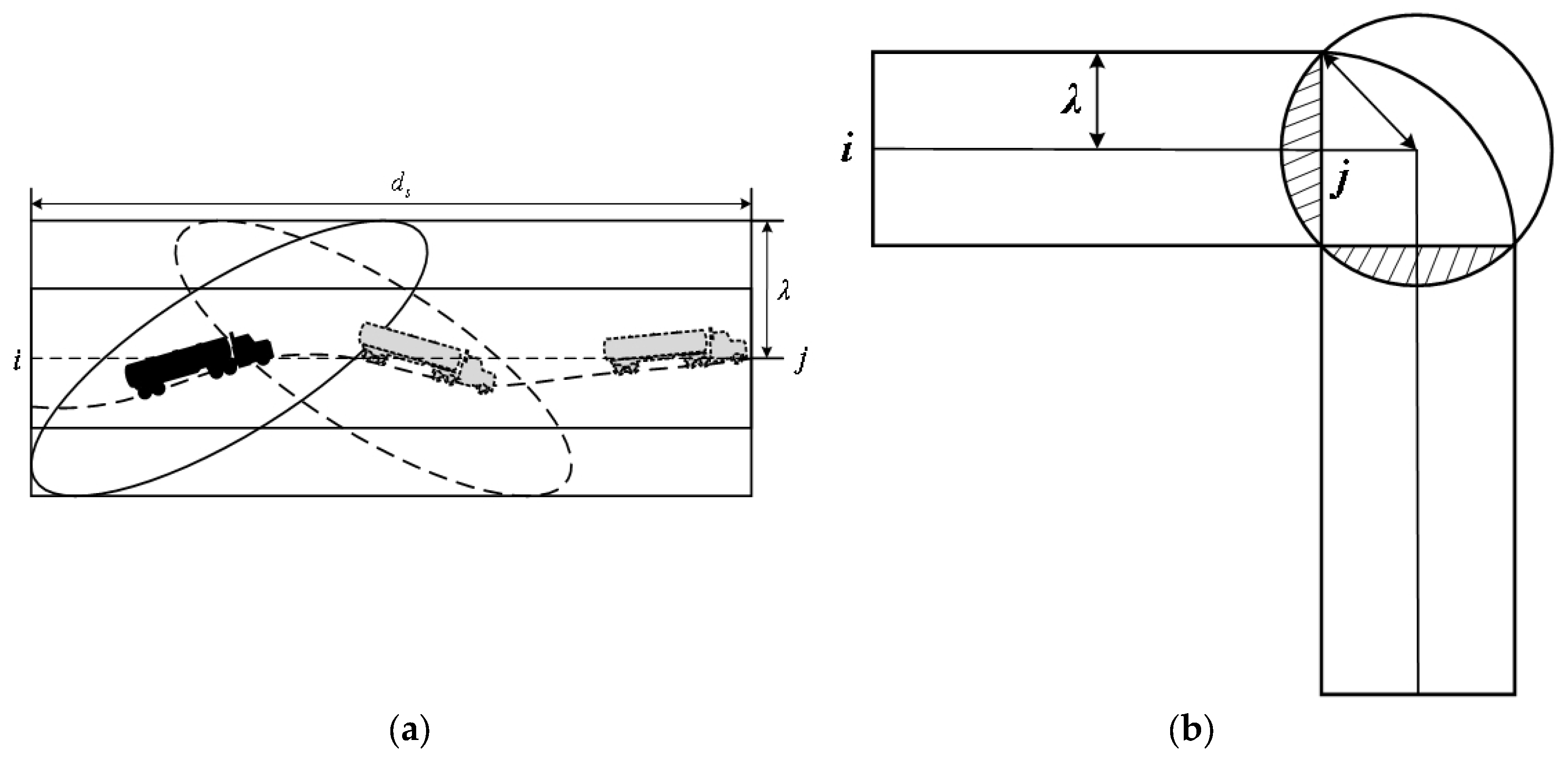
Given the inevitability of lane-changing maneuvers, a vehicle’s transportation trajectory is never a straight line. Therefore, there are multiple possibilities for vehicles’ motion patterns on straight segments, and the influence district is approximated as a rectangle in this study, shown in Figure 2a. Therefore, the exposure area of the straight road is obtained as
s 1 = 2 λ d s .
For convenience, this study approximates the impact area when the vehicle passes through a curve as a circle. According to the ratio of the accident probability on the curve to the accident probability on the main road, the radius of this circular coverage area is determined to be 2 λ , as shown in Figure 2b; the exposed area of the curved segment is affected by the error caused by the overlap with the straight segments. Therefore, the exposure area of the curved road is obtained as
s 2 = π 2 λ 2 2 λ λ 2 λ 2 x 2 d x .
According to field experience, when vehicle k is traveling on road segments, the number of people affected by a hazmat accident is given as
p o p 1 = s S x s k μ s s 1 ,
p o p 2 = c C x c k μ c s 2 .
In addition to the aforementioned factors, the vehicle load weight, which constantly changes during the transportation process, is considered here. By combining the weight coefficients, the cumulative risk of vehicles for the driving route during the transportation process is given as
R k = ω 1 s r s p 1 p o p 1 q s k Q β + ω 2 c r c p 2 p o p 2 q c k Q β .
And the total risk of the hazmat vehicle routing problem is given as
f 2 = ω 1 k K s r s p 1 x s k μ s s 1 q s k Q β + ω 2 k K c r c p 2 x c k μ c s 2 q c k Q β
According to Equations (8) and (14), the optimization model on HVRP-DRC is structured as
min f 1 = k K c 1 + c 2 + c 3 + 2 c 4 + c 5 ω 1 F 1 + ω 2 F 2 + c 6 φ ω 1 F 1 + ω 2 F 2 ,
min f 2 = ω 1 k K s r s p 1 x s k μ s s 1 q s k Q β + ω 2 k K c r c p 2 x c k μ c s 2 q c k Q β .
Subject to
0 q i k Q , i N 0 , k K ,
q j k 0 , j N \ N 0 , k K ,
k K j N \ N 0 x 0 j k K ,
k K j N \ N 0 x j 0 k K ,
k K j N , i j x i j k = 1 , i N n ,
0 < q n Q , n N n ,
x s k 0 , 1 ,
x c k 0 , 1 .
Here, constraints (17) and (18) impose restrictions on vehicle loading capacity. Constraint (17) ensures that the loaded weight upon departure from the depot does not exceed the vehicle’s maximum capacity. Constraint (18) guarantees non-negative remaining load when leaving customer nodes. Constraints (19) and (20) specify that the number of transportation routes cannot surpass the available fleet size. Constraint (21) enforces single-visit service for all customers. Constraint (22) requires customer demands to be positive and smaller than the vehicle’s maximum capacity. Finally, Constraints (23) and (24) define the binary decision variables.

3. Solution Approach

This section introduces the solution process of the optimization model. Specifically, Section 3.1. describes the multi-objective optimization algorithm used, and Section 3.2. introduces the detailed steps of the algorithm to solve the HVRP-DRC model.

3.1. Ant Colony Algorithm

Currently, the solution methods for VRP are mainly divided into exact algorithms and heuristic algorithms. However, the proposed HVRP-DRC model, which involves a large number of complex constraints, poses significant challenges for the application of exact algorithms. In contrast, heuristic algorithms, such as the ACO algorithm and Particle Swarm Optimization (PSO) algorithm, stand out due to their simplicity and fast convergence speed. Therefore, this study adopts the ACO algorithm to solve the proposed model. Algorithm 1 shows the pseudo-code of the ACO algorithm.
In the algorithm, N represents the iterations; M represents the number of ants; d i j denotes the distance between nodes i and j, and τ i j ( t ) indicates the pheromone concentration between nodes i and j at time t. Initially, the pheromone concentration on each path is identical, i.e., τ 0 = C (where C is a constant), and p i j ( m ) represents the probability of the m-th ant transitioning from node i to the next node j, which is expressed as
p i j ( m ) = τ ( i , j ) α η ( i , j ) β j J m ( i ) τ ( i , j ) α η ( i , j ) β ,   if   j J m ( i ) , 0 ,   otherwise .
Here, τ ( i , j ) represents the concentration value of the pheromone between nodes i and j; J m ( i ) represents the set of available nodes at node i for ant m, and η ( i , j ) = 1 d i j .
After each iteration, the pheromones along the road segments are updated again based on their accumulation and evaporation levels. The calculation formula is as follows:
τ i j ( t + 1 ) = ( 1 ρ ) τ i j ( t ) + Δ τ i j ( t , t + 1 ) ,
Δ τ i j ( t , t + 1 ) = m = 1 M Δ τ i j m ( t , t + 1 ) ,
Δ τ i j m ( t ) = Q L m ,   if   ( i , j )   traversed   by   ant   m , 0 ,   otherwise .
Here, ρ is the volatility factor of pheromone, and its value lies within the range of [0,1]; τ i j ( t ) represents the amount of pheromone between nodes i and j during each iteration; Δ τ i j ( t , t + 1 ) represents the total amount of pheromone concentration of all ants on the path from node i to j in this iteration; Q represents the intensity of pheromone; L m represents the total length of the path traversed by ant m.
Algorithm 1 The pseudo-code of the ACO algorithm
 Algorithm: Ant Colony Optimization (ACO)
1:Input:
2:Number of ants ( m );
3:Number of iterations ( m a x _ i t e r );
4:Pheromone evaporation rate;
5:Pheromone influence factor;
6:Initial pheromone level ( τ 0 );
7:Number of objectives ( K );
8:Output:
9:Best solution.
10:Begin:
11:Initialize:
12:Set pheromone levels τ i j t = τ 0 for all edges i , j ;
13:Initialize Pareto archive A = ;
14:Set b e s t _ s o l u t i o n s = ;
15:For  i t e r a t i o n  to  m a x _ i t e r :
16:For each ant k to  m :
17:  Put ant k on the starting node;
18:  While the ant has not visited all nodes:
19:   Choose the next node j from unvisited nodes with probability;
20:   Move ant k to node j ;
21:   Mark node j as visited;
22:   Evaluate the solution on the distance;
23: Update pheromone levels;
24: Update the global optimal solution;
25:Return Best solution.
26:End Begin
For the traditional ACO algorithm, the advantage lies in optimizing routes to ensure the shortest travel route. However, due to the complex road network between depot and customer nodes, the routes optimized by the traditional ACO algorithm often exhibit excessive cumulative turning angles and redundant road segments. Considering the large size of tanker trucks transporting hazmat, such routes are not vehicle-friendly, increasing safety risks during hazmat transportation and reducing transport efficiency. To address these issues, this study improves the TSACO algorithm, including enhancements to the node probability selection, pheromone update mechanism, and route optimization strategies.

3.2. Improved Node Probability Selection

To prevent the algorithm from converging to local optima, an enhanced node probability selection strategy is proposed for ant path selection, which is formulated as
s i j ( m ) = arg max τ i , j α η i , j β ,   if   q < q 0 , p i j m ,   otherwise .
Here, s i j ( m ) denotes the probability of ant m transitioning from node i to node j; q represents a random variable uniformly distributed in [0,1]; and q 0 represents the threshold probability determining whether the ant employs deterministic selection or roulette wheel selection. Specifically, if q < q 0 , the ant transitions to the node with the maximum heuristic value; otherwise, it calculates the selection probabilities for all feasible nodes and performs roulette wheel selection.
Evidently, q 0 plays a pivotal role in next-node selection. Consequently, an adaptive adjustment mechanism for q 0 is introduced, formulated as
q 0 = q 0 · e n ,   if   more   than   half   of   the   solutions   are   the   same , 0.1 + 2 n 0.45 N 2 N 2 ,   otherwise .
During the initial phase of the algorithm execution, ants are assigned a higher probability for deterministic node transitions to accelerate the search for local optima. In later iterations, to prevent the generation of multiple duplicate solutions, the probability of stochastic roulette wheel selection is progressively increased. This probability grows monotonically with the number of iterations, thereby enhancing the algorithm’s exploratory capability in the solution space.

3.3. Improved Pheromone Update Strategy

In the ACO algorithm, pheromone updating is a crucial process. When pheromone interference on sub-optimal paths prevents ants from finding the optimal path, the algorithm falls into local optima. This is particularly prone to occur during later iterations. To enhance the algorithm’s global search capability and increase path optimization diversity in later iterations, this study introduces a dynamic adjustment method of pheromone evaporation rate. It is noteworthy that the pheromone updating is structured by using five formulas, among which the formula on evaporation rate is borrowed from Liu et al. [30].
Specifically, the rank-based optimization mechanism sorts all ant paths according to their fitness values after each iteration. Higher rankings indicate better path quality. To guide ants to preferentially select high-quality paths with greater pheromone concentration in subsequent iterations, pheromone weighting is applied based on path rankings, thereby increasing pheromone concentration on superior path segments. Meanwhile, following the elite ant mechanism, the ants are sorted from largest to smallest according to the fitness value, and only the top s-ranked ants are permitted to deposit pheromones. The improved pheromone update formula is
τ i j ( t + 1 ) = ( 1 ρ ) τ i j ( t ) + Δ τ i j ( t , t + 1 ) ,
ρ = ρ 0 · 1 + 0.2 n N ,
Δ τ i j ( t , t + 1 ) = m = 1 s w m · Δ τ i j m ( t , t + 1 ) ,
w m = 1 + e λ m 1 ,
Δ τ i j m ( t ) = Q f i t n e s s ,   if   ( i , j )   traversed   by   ant   m , 0 ,   otherwise .
Here, ρ 0 is the initial value of ρ ; ρ 0 = 0.3 ; ρ increases with the increase in iteration times n, and in the later stage of iteration, the rate of pheromone volatilization accelerates, expanding the search space of the ant colony; w m is the exponential decay weight for ant ranking, λ is the attenuation coefficient, which is 0.2; f i t n e s s = f 1 + f 2 2 .
Thus, this study improves the encoding method of the algorithm by numbering all the endpoints of the route. The vehicle route encoding now includes not only the sequence numbers of the endpoints of the traveled roads but also the numbers of the customer nodes visited along the route.

3.4. Algorithm Implementation Process

Based on the main description of the algorithm, the solution steps for the proposed HVRP-DRC model are as follows. Then, the flowchart of the proposed TSACO algorithm is shown in Figure 3.
Step 1: Initialize parameters.
Set parameters such as the ant colony size, pheromone importance factor, heuristic function importance factor, pheromone evaporation factor, total pheromone release, and maximum number of iterations. Label all vertices in the undirected graph and construct the distance matrix and pheromone matrix between vertices. Furthermore, in order to distinguish the IDs of the customer nodes from those of the road section points, the IDs of the customer nodes are encoded by adding 1000 to them.
Step 2: Start the first stage of the algorithm.
Calculate the optimal path between two nodes, including the customer node. Replace shortest distance with fitness and use the Dijkstra algorithm to calculate the optimal path and store it. In the HVRP-DRC model, the travel route between two nodes for a vehicle is no longer simply approximated by the Euclidean distance. Instead, it takes into account the actual road conditions during vehicle transportation, including the number of times the vehicle travels straight and turns. After the path calculations for all nodes have been completed, the next stage will be entered.
Step 3: Find the next customer node.
The ant departs from the depot and calculates all customer nodes satisfying the constraint conditions, storing them in a candidate set. If the set is empty, the ant returns to the depot. Otherwise, the ant selects the next customer node based on the pheromone concentration on each route. To help the algorithm escape local optima, the algorithm employs an improved probability selection strategy to select the next customer node.
Step 4: Ant path update.
After selecting the next customer node, the ant updates its current route based on the actual driving route determined by Dijkstra’s algorithm, incorporating all segment information between customer nodes along the vehicle’s travel route.
Step 5: Pheromone update.
The global update of all vehicle routes is carried out based on the improved pheromone update strategy.
Step 6: Update the optimal solution.
Compare with the optimal solution of the previous iteration and update the global optimal solution. After all updates are completed, the pheromone and other information of ants are reset to prepare for the next round of iteration.
Step 7: Output results.
On the condition that the iteration times reach a given number, the best solution is stored while the iterative process is output. Here, the stored set includes information concluding the travel routes, bi-objective function values, and the number of vehicles used.

4. Application Example

This section contains four subsections, as follows. Section 4.1. delineates the selected validation cases and algorithmic parameters employed. Section 4.2. conducts a comparative analysis of the algorithm’s problem-solving performance. Section 4.3. performs sensitivity analysis on critical parameters influencing vehicular transportation risk within the proposed model. Section 4.4. demonstrates the effectiveness of the proposed TSACO algorithm by using 12 modified Solomon benchmark instances. Section 4.5. synthesizes findings from existing research to evaluate this model, discussing both its innovative advantages and inherent limitations. Moreover, to ensure the objectivity of the experiment, the TSACO algorithm was implemented under an Intel Core i5-13500H 2.60 GHz computer with a Windows 11 environment.

4.1. Data Collection

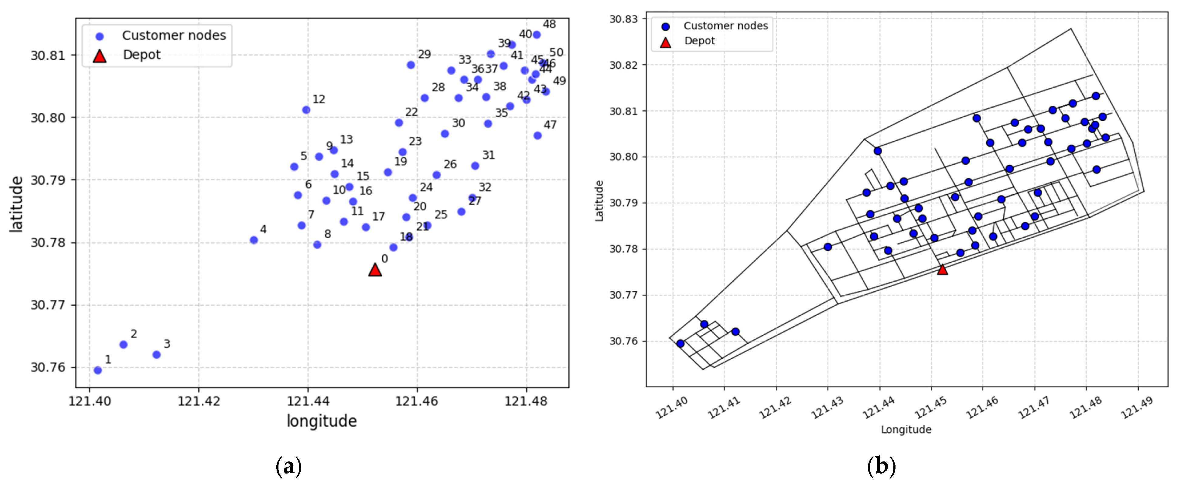
Assume that there is a port chemical industrial park, and assume that there is a type of liquid hazmat to be delivered to 50 enterprises daily. The parameters on vehicle transportation and the park are collected from safety experts and truck drivers and are listed in Table 2. Assume that there are 50 enterprises (customer nodes) that require transportation services. All the enterprises, as well as all the endpoints of the available road sections in the introduced park, are numbered, following a top-to-bottom and left-to-right order. Specifically, the locations of the customer nodes are depicted in Figure 4a, while the park’s road network is illustrated in Figure 4b.
For convenience, a series of assumptions is made as follows. First, all transport segments in Figure 4b are depicted as straight lines. Second, service time windows for enterprises are not considered, and the range of the demand amounts of each enterprise is converted to 0,10. Third, the weight of the two optimal objects, i.e., the cost and risk values, is equal. Under the aforementioned conditions, the question is to find an optimal routing solution for vehicles using Equations (15)–(24), to minimize the cost and risk values.

4.2. Calculation and Analysis

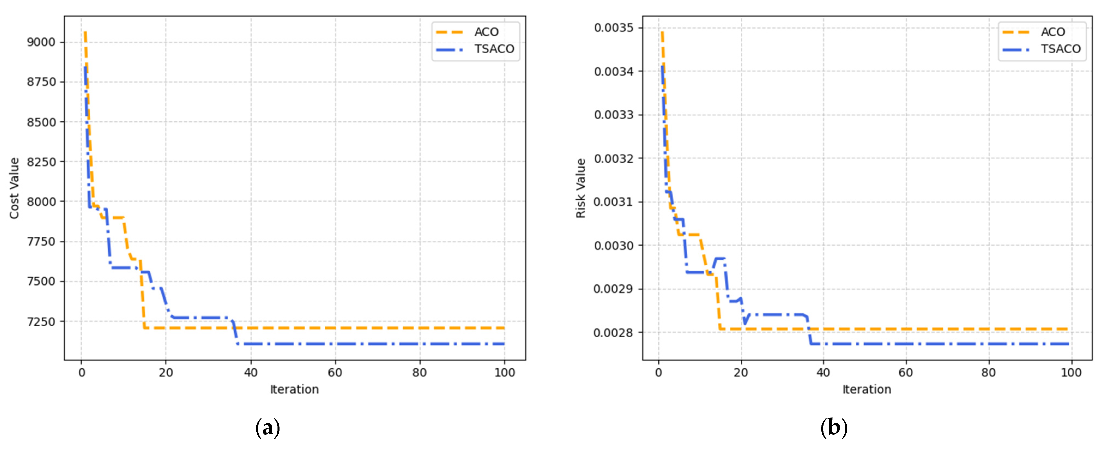
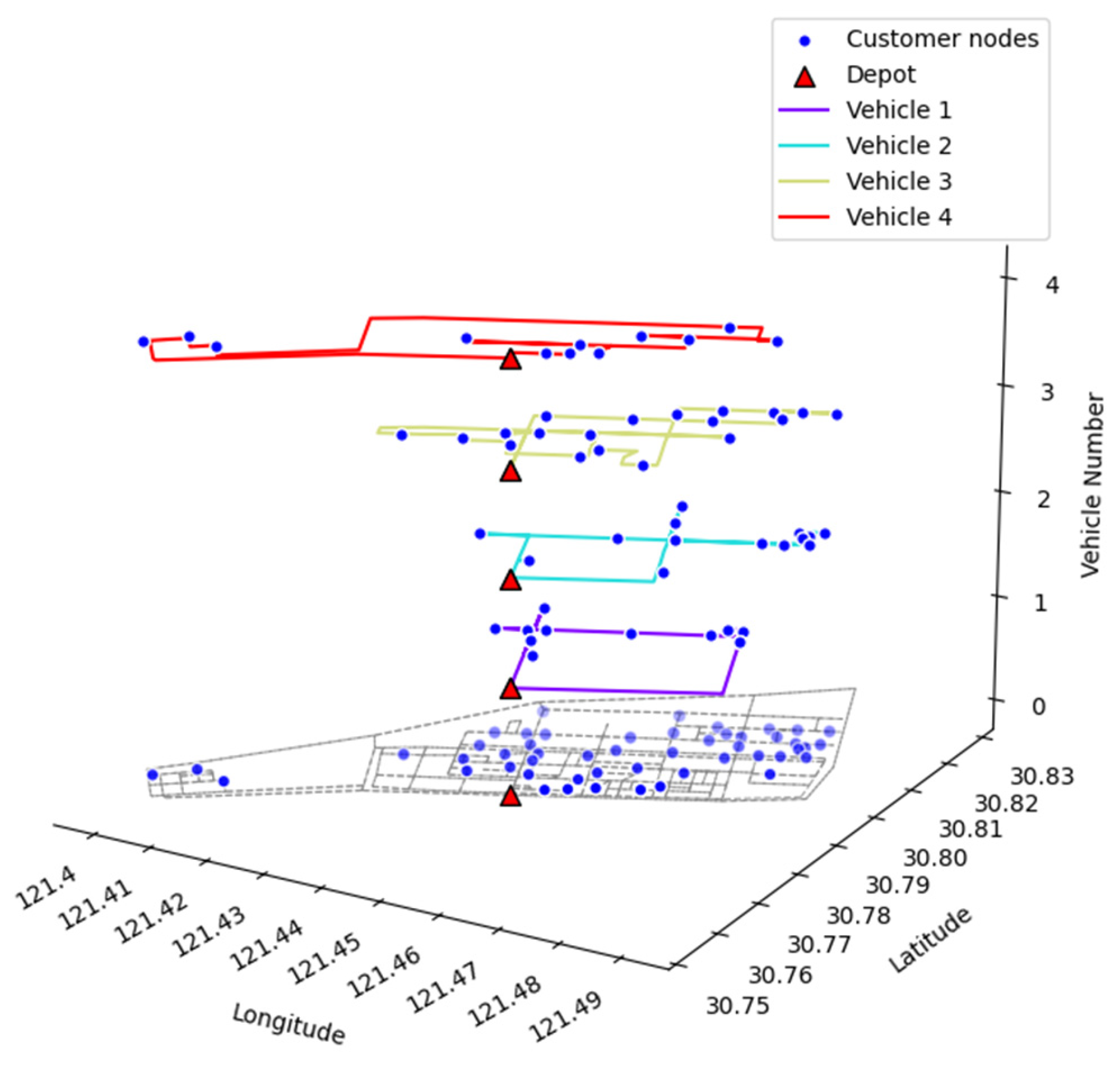
To obtain a hazmat transportation method that optimally balances both transport risk and cost in actual life, this study employs the TSACO algorithm to conduct a numerical experiment on the proposed model for a port chemical industrial park. The algorithm is executed randomly ten times, with each run generating an optimal solution. Meanwhile, a classical ACO algorithm is employed to optimize vehicle routing for customer node service. After ten independent runs, the optimal solutions from both algorithms were selected for comparison. Figure 5 presents the comparative results of objective function values between the ACO and TSACO algorithms when reaching the maximum iteration limit. Table 3 presents the detailed calculation results obtained by using the two aforementioned algorithms. The vehicle routes obtained by using the TSACO algorithm are shown in Figure 6, and the detailed path information is presented in Table 4.
Based on the obtained calculation results, a series of analyses is given as follows:
(1)
Figure 5 reveals that during the early stages (iterations 1–20), the ACO algorithm demonstrates faster convergence rates. However, its performance plateaus upon reaching a certain threshold. In contrast, the TSACO algorithm exhibits initial fluctuations in objective values but ultimately achieves superior solutions through continued iterations. These results indicate that while the ACO algorithm shows rapid initial optimization, it becomes trapped in local optima.
(2)
Table 3 presents the detailed data obtained by the two algorithms, including the number of vehicles, total cost, total risk, and the running time of the algorithms. Additionally, the discrepancy between the objective values of these feasible solutions is quantified using a formulated calculation method, i.e., s ACO s TSACO s ACO × 100 % . The results demonstrate significant quality improvements in both total transportation cost (1.38%) and total risk (1.21%) metrics for the optimized solutions, obtained by using the proposed model. It is noteworthy that the modified algorithm requires more computational time compared to the conventional ACO due to its additional calculation steps. This temporal overhead represents a trade-off between solution quality and computational efficiency, which is common in metaheuristic algorithm improvements. However, as the computational complexity decreases, the running times of the two models show a convergence trend. The 12 examples proposed in Section 4.4. to verify this regulation.

4.3. Sensitivity Analysis

Prior to conducting specific sensitivity analysis, key parameters and their value ranges are introduced as follows. In the classical ACO algorithm, the core calculation lies in node selection and pheromone update. During the pheromone update phase, the pheromone evaporation rate governs the speed of pheromone dissipation, thereby influencing the algorithm’s exploration capability. Meanwhile, the proposed TSACO algorithm introduces a dynamic pheromone evaporation rate that varies with iteration count. To analyze the impact of ρ 0 values on algorithm optimization, nine parameter values from 0.1 to 0.9 in increments of 0.1 are tested, with each parameter executed ten times. The calculation results are shown in Figure 7.
In Figure 7a,b, the coefficient ρ 0 demonstrates a non-monotonic influence on algorithm performance. The optimal cost and risk exhibit a characteristic pattern of initial decrease, followed by an increase and subsequent decrease as ρ 0 grows. Specifically, at lower ρ 0 values (0.1–0.3), both cost and risk exhibit minimal fluctuations where the algorithm, constrained by excessive pheromone accumulation, demonstrates enhanced local search capability leading to relatively lower cost–risk values. When ρ 0 reaches intermediate levels (0.4–0.5), intensified evaporation reduces the path dependence of the proposed model while enhancing its exploration capability. Further increase to ρ 0 = 0.6–0.9 causes premature pheromone dissipation before effective utilization, inducing random search behavior that degrades convergence performance and generates significant cost–risk fluctuations.
Moreover, for each set value ρ 0 0.1 ,   0.2 ,   ,   0.9 , set the execution times to 10. After eliminating the outliers or abnormal calculation results, nine boxpoints are obtained to describe the optimal cost values, and nine represent optimal risk values. More details are shown in Figure 7c,d. It is noteworthy that the highest point at the end of each vertical box represents the maximum optimized value for each ρ 0 obtained from 10 calculations (after excluding outliers). Similarly, the lowest point at the end of each vertical box represents the minimum values. The boxplots in Figure 7c,d demonstrate superior overall performance at lower ρ 0 values (particularly 0.1–0.3). As the parameter ρ 0 increases, the quality of the calculation results gradually deteriorates. Therefore, preventing extreme pheromone accumulation while maintaining stable performance ρ 0 = 0.3 is recommended as the optimal configuration. In general, the regulations derived from Figure 7c–d are consistent with those from Figure 7a,b, which verifies the validity of the sensitivity analysis.

4.4. Algorithm Validation

To demonstrate the effectiveness of the proposed algorithm, 12 modified Solomon benchmark instances, which are located in three districts (namely, C, R, and RC), are employed [31]. Specifically, 12 chosen VRP with time windows instances are transformed into CVRP since that time window is not considered in this study. The geographical attributes of the proposed instances are different, where two instances are adopted for type C, type R, and type RC, respectively. Furthermore, each instance is divided into medium-scale and small-scale subsets for calculation.
This study conducted comparative validation between the proposed TSACO algorithm and the conventional one, with detailed solution results for different instances presented in Table 5. In particular, since there is no pathway information between each customer node in the adopted instances, the distance between each node is calculated by using Euclidean distances. For clarity, Figure 8 presents the box plots for instances C101-25, C101-50, R101-25, R101-50, RC101-25, and RC101-50.
The optimized results presented in Table 5 include the required number of vehicles for each instance, the shortest travel distance achieved, and the deviation between the two algorithms. Specifically, the obtained results show that the TSACO algorithm yields superior solutions to the conventional one in most cases. For specific comparison results, please refer to Figure 8. In essence, the success of the proposed TSACO algorithm is attributed to Equations (29) and (30), where node selection ability is enhanced.

4.5. Discussion

This study applies the TSACO algorithm to both twelve CVRP instances and a simulation case using survey parameters for comprehensive comparative analysis. In benchmark experiments, the shortest transportation distances obtained by both algorithms demonstrate that TSACO consistently achieves superior convergence results compared to conventional ACO, confirming the efficacy of the two proposed improvement mechanisms in enhancing ACO’s performance. Furthermore, the algorithm maintains robust performance across varying customer node distributions, verifying its generalizability. Then, for the port chemical park simulation case, the optimized solutions generated by TSACO exhibit significant advantages in both transportation risk mitigation (average 1.38%) and cost efficiency (1.21%), empirically validating the effectiveness of the proposed hazardous material vehicle routing optimization methodology.
Unlike conventional approaches, this HVRP-DRC model accounts for the influence of uncertainty factors across different road segments on overall transportation risk, resulting in safer and more rational transportation routes. Furthermore, for practical applications, the model does not simply treat inter-node transportation distances as Euclidean distances but rather investigates actual road conditions within port chemical industrial parks. The Pareto optimal solutions obtained through the TSACO algorithm provide crucial flexibility for transportation managers to select appropriate optimization schemes based on real-world requirements.
Although this case study obtained meaningful results, certain limitations remain. Based on an extensive survey of road conditions within port chemical industrial parks, this study established the model by using a grid-based road network. However, in actual transportation scenarios, the direction of the vehicle’s steering when it is on a curved road also affects the transportation risk. Additionally, the uncertain factors affecting the accident probability of curved segments prove difficult to quantify. The model still faces challenges when analyzing how different factors influence transportation risks.

5. Conclusions

Considering different road conditions for hazmat transportation in port chemical industrial parks, this study proposes a bi-objective HVRP-DRC model that incorporates curve section transportation risks into vehicle route optimization. Furthermore, the reliability of the proposed model in practice is validated by simulation experiments. The main conclusions are summarized as follows.
First, road conditions are classified into straight segments and curved segments. A comprehensive risk quantification model is proposed by incorporating exposure areas into the risk under different road conditions, which reduces the risk and cost. This suggests that geometric segmentation of transportation networks is a valuable modeling principle for other logistics contexts involving risk-sensitive vehicles.
Second, the consistent improvements in both cost and risk metrics across benchmark datasets and a simulation case using survey parameters indicate that the TSACO algorithm’s two-stage structure is an effective template for tackling other multi-constraint, bi-objective routing problems. The stability of these improvements across different problem instances implies that the method is robust to variations in node demand distribution.
Third, this study highlights the value of integrating safety considerations into routing optimization as an objective of equal importance to economic efficiency. By adopting a weighted sum of transportation cost and risk, complemented by a predefined risk threshold, the model produces a balanced routing plan that meets operational efficiency targets while ensuring that risk remains within acceptable limits. This structure enables decision-makers to implement optimization results directly, thereby enhancing the practicality and enforceability of transportation management in real-world hazmat transportation planning.
Nevertheless, this study has certain limitations. Accident probabilities for curved segments are influenced by multiple uncertain factors that remain difficult to measure precisely. And the current model does not incorporate real-time vehicle speed or weather, which enhances responsiveness in dynamic environments. Future research will address these limitations by (1) integrating stochastic demand and uncertain supply scenarios into the optimization framework; (2) considering the impact of real-time vehicle speed and dynamic environment on transportation; and (3) extending the approach to multi-modal hazmat transportation and complex logistics networks. Furthermore, the proposed methodology is adaptable to a variety of routing contexts, including urban hazardous waste collection and emergency evacuation planning.

Author Contributions

Conceptualization, F.Z. and L.D.; methodology, L.D.; software, L.D.; validation, J.J. and F.K.; formal analysis, F.Z.; investigation, X.L.; resources, L.D.; data curation, L.D.; writing—original draft preparation, L.D.; writing—review and editing, F.Z.; visualization, L.D.; supervision, F.Z.; project administration, F.Z.; funding acquisition, F.Z. All authors have read and agreed to the published version of the manuscript.

Funding

This research was funded by the Natural Science Foundation of Shandong Province, grant number ZR2021MG003, and the Humanities and Social Sciences Foundation of the Ministry of Education of the People’s Republic of China, grant number 24YJA880087. The APC was funded by Fangwei Zhang.

Data Availability Statement

The data presented in this study are available on request from the corresponding author.

Conflicts of Interest

The authors declare no conflicts of interest.

References

  1. Lyu, S.; Zhang, S.H.; Huang, X.M.; Peng, S.N.; Li, J. Investigation and modeling of the LPG tank truck accident in Wenling, China. Process Saf. Environ. Prot. 2022, 157, 493–508. [Google Scholar] [CrossRef]
  2. Oyugi, B.; Kamara, I.F.; Nuwagira, I.; Musoke, R.; Lakoh, S.; Jalloh, A.; Kamara, R.F.; Relan, P.; Lajolo, C.; Ndiaye, R.A.M.; et al. A review of the response and the emergency medical team (EMT) deployment following a tanker explosion in Freetown, Sierra Leone. Confl. Health 2024, 18, 63. [Google Scholar] [CrossRef] [PubMed]
  3. Elvik, R. The more (sharp) curves, the lower the risk. Accid. Anal. Prev. 2019, 133, 105322. [Google Scholar] [CrossRef] [PubMed]
  4. Jiang, Q.K.; Wang, H.K. Risk assessment and hybrid algorithm transportation path optimization model for road transport of dangerous goods. IATSS Res. 2025, 49, 72–80. [Google Scholar] [CrossRef]
  5. Shankar, V.; Mannering, F.; Barfield, W. Effect of roadway geometrics and environmental factors on rural freeway accident frequencies. Accid. Anal. Prev. 1995, 27, 371–389. [Google Scholar] [CrossRef]
  6. Maji, S.; Maity, S.; Giri, D.; Nielsen, I.; Maiti, M. Multi-objective multi-path COVID-19 medical waste collection problem with type-2 fuzzy logic based risk using partial opposition-based weighted genetic algorithm. Eng. Appl. Artif. Intell. 2025, 143, 109916. [Google Scholar] [CrossRef]
  7. Zhai, C.L.; Li, P.L.; Zhao, R.H.; Jing, N.N. Selection and planning of hazardous materials transportation routes based on explosion accident risks. J. Loss Prev. Process Ind. 2024, 92, 105440. [Google Scholar] [CrossRef]
  8. Xie, L.; Cao, C.X. Multi-modal and multi-route transportation problem for hazardous materials under uncertainty. Eng. Optim. 2020, 53, 2180–2200. [Google Scholar] [CrossRef]
  9. Zandieh, F.; Ghannadpour, S.F. A comprehensive risk assessment view on interval type-2 fuzzy controller for a time-dependent hazmat routing problem. Eur. J. Oper. Res. 2023, 305, 685–707. [Google Scholar] [CrossRef]
  10. Wang, J.P.; Bai, X.J.; Liu, Y.K. Building sustainable hazardous products supply chain against ambiguous risk with accelerated Benders decomposition algorithm. Transport. Res. E-Log. 2025, 194, 103941. [Google Scholar] [CrossRef]
  11. Kang, D.; Zhao, J.X.; Dick, C.T.; Liu, X.; Bian, Z.Y.; Kirkpatrick, S.W.; Lin, C.Y. Probabilistic risk analysis of unit trains versus manifest trains for transporting hazardous materials. Accid. Anal. Prev. 2023, 181, 106950. [Google Scholar] [CrossRef]
  12. Li, G.Q.; Pu, G.; Yang, J.X.; Jiang, X.G. A multidimensional quantitative risk assessment framework for dense areas of stay points for urban hazmat vehicles. Reliab. Eng. Syst. Saf. 2024, 241, 109637. [Google Scholar] [CrossRef]
  13. Chiou, S.W. A learning optimization for resilience enhancement of risk-informed traffic control system with hazardous materials transportation under uncertainty. Reliab. Eng. Syst. Saf. 2024, 252, 110425. [Google Scholar] [CrossRef]
  14. Zhan, H.F.; Wang, G.; Shan, X.; Liu, Y.H. Risk-aware lane-change trajectory planning with rollover prevention for autonomous light trucks on curved roads. Mech. Syst. Signal Proc. 2024, 211, 111126. [Google Scholar] [CrossRef]
  15. Zheng, X.L.; Yu, L.J.; Ren, Y.Y.; Li, X.S.; Liang, B.; Xi, J.F. Modeling of tank vehicle rollover risk assessment on curved-slope combination sections for sustainable transportation safety. Sustainability 2025, 17, 906. [Google Scholar] [CrossRef]
  16. Wang, T.; Ge, Y.E.; Wang, Y.J.; Chen, W.Q.; Qian, F.; Niu, Y.C. A novel model for real-time risk evaluation of vehicle–pedestrian interactions at intersections. Accid. Anal. Prev. 2024, 206, 107727. [Google Scholar] [CrossRef] [PubMed]
  17. Ma, H.Z.; Qian, C.; Li, L.H.; Qu, X.; Ran, B. Risk quantification based Adaptive Cruise control and its application in approaching behavior at signalized intersections. Accid. Anal. Prev. 2025, 212, 107939. [Google Scholar] [CrossRef]
  18. Zhai, C.L.; Wu, A.Z. Probabilistic risk analysis and characterization of hazardous material road transportation routes under explosion accidents. J. Loss Prev. Process Ind. 2024, 88, 105265. [Google Scholar] [CrossRef]
  19. Yang, J.G.; Zhuang, Y.B. An improved ant colony optimization algorithm for solving a complex combinatorial optimization problem. Appl. Soft Comput. 2010, 10, 653–660. [Google Scholar] [CrossRef]
  20. Zhou, X.S.; Gui, W.Y.; Heidari, A.A.; Cai, Z.N.; Liang, G.X.; Chen, H.L. Random following ant colony optimization: Continuous and binary variants for global optimization and feature selection. Appl. Soft Comput. 2023, 144, 110513. [Google Scholar] [CrossRef]
  21. Wang, T.C.; Wang, L.; Li, D.D.; Cai, J.C.; Wang, Y.X. Monte Carlo-based improved ant colony optimization for path planning of welding robot. J. King Saud Univ.-Comput. Inf. Sci. 2023, 35, 101603. [Google Scholar] [CrossRef]
  22. Zhang, X.; Hao, Y.C.; Zhang, L.Y.; Yuan, X.M. Application of improved genetic algorithm to vehicle routing problem considering the environmental self-regulation of the freight companies. Expert Syst. Appl. 2025, 274, 127010. [Google Scholar] [CrossRef]
  23. Sarbijan, M.S.; Behnamian, J. Multi-fleet feeder vehicle routing problem using hybrid metaheuristic. Comput. Oper. Res. 2022, 141, 105696. [Google Scholar] [CrossRef]
  24. Shi, X.W.; Yao, H.D.; Liang, Z.H.; Li, X.P. An empirical study on fuel consumption of commercial automated vehicles. Transp. Res. Part D Transp. Environ. 2022, 106, 103253. [Google Scholar] [CrossRef]
  25. Gao, C.; Xu, J.L.; Jia, M.; Sun, Z.H. Correlation between carbon emissions, fuel consumption of vehicles and speed limit on expressway. J. Traffic Transp. Eng. 2024, 11, 631–642. [Google Scholar] [CrossRef]
  26. Li, T.T.; Deng, S.J.; Lu, C.Y.; Wang, Y.; Liao, H.J. Optimization of Green Vehicle Paths Considering the Impact of Carbon Emissions: A Case Study of Municipal Solid Waste Collection and Transportation. Sustainability 2023, 15, 16128. [Google Scholar] [CrossRef]
  27. Ma, T.M.; Wang, Z.; Yang, J.L.; Huang, C.Y.; Liu, L.J.; Chen, X.F. Real-time risk assessment model for hazmat release accident involving tank truck. J. Loss Prev. Process Ind. 2022, 77, 104759. [Google Scholar] [CrossRef]
  28. Chakrabarti, U.K.; Parikh, J.K. Route evaluation for hazmat transportation based on total risk–a case of Indian state highways. J. Loss Prev. Process Ind. 2011, 24, 524–530. [Google Scholar] [CrossRef]
  29. Bejleri, I.; Xu, X.J.; Silva, K.R.; Srinivasan, S. Safety performance analysis of horizontal curves in urban areas. Accid. Anal. Prev. 2024, 195, 107402. [Google Scholar] [CrossRef]
  30. Liu, C.; Wu, L.; Xiao, W.S.; Li, G.X.; Xu, D.P.; Guo, J.J.; Li, W.T. An improved heuristic mechanism ant colony optimization algorithm for solving path planning. Knowl.-Based Syst. 2023, 271, 110540. [Google Scholar] [CrossRef]
  31. Solomon, M.M. Algorithms for the vehicle routing and scheduling problems with time window constraints. Oper. Res. 1987, 35, 254–265. [Google Scholar] [CrossRef]
Figure 1. The primary processes of this study.
Mathematics 13 02690 g001
Figure 2. (a) Affected area in straight segment; (b) Affected area in curved segment.
Mathematics 13 02690 g002
Figure 3. Flowchart of the TSACO algorithm.
Mathematics 13 02690 g003
Figure 4. (a) Customer node location map; (b) The grid map of the paths in the port chemical industrial park.
Mathematics 13 02690 g004
Figure 5. (a) Total cost value for each iteration; (b) Total risk value for each iteration.
Mathematics 13 02690 g005
Figure 6. Vehicle transportation route map.
Mathematics 13 02690 g006
Figure 7. The sensitivity analysis results of the volatilization rate of pheromones: (a) The minimum cost values obtained with different parameters; (b) The risk value corresponding to the minimum cost value; (c) Boxplot of cost values; (d) Boxplot of risk values.
Mathematics 13 02690 g007
Figure 8. Boxplots of the 101 instances of types C, R, and RC: (a) C101-25; (b) C101-50; (c) R101-25; (d) R101-50; (e) RC101-25; (f) RC101-50.
Mathematics 13 02690 g008aMathematics 13 02690 g008b
Table 1. Model parameters and variables.
SymbolDefinition
NSet of all nodes in the studied road network
N 0 The depot within the port-based chemical industrial park
N n Set   of   customer   nodes ,   N n = 1 , 2 , , n
N z Set   of   all   intersections   on   road   segments ,   N z = 1 , 2 , , z
S Set   of   straight   road   segments ,   S E
C Set   of   curved   road   segments ,   C E
K Set   of   all   transport   vehicles ,   K = 1 , 2 , , k
QVehicle rated load capacity
Q e Vehicle empty load capacity
Q a Actual vehicle load capacity
q n The demand of customer node n
R Set   of   vehicle   transportation   routes ,   R = 1 , 2 , , r
r n Set   of   customer   nodes   traversed   by   route   r ,   r n N n
r s Set   of   straight   road   segments   s   traversed   in   route   r ,   r s S
r c Set   of   curved   road   segments   c   traversed   in   route   r ,   r c C
d s The   distance   of   straight   road   segment   s ,   s S
d c The   distance   of   curved   road   segment   c ,   c C
σ Fuel consumption rate of the vehicle when it is empty (L/h)
θ Vehicle steering angle (°)
v 1 The average speed of the vehicle when traveling on straight road
v 2 The average speed of the vehicle when traveling on curved road
φ Carbon emission factor
μ s Population density on road segment s
μ c Population density on road segment c
c 1 Vehicle rental cost
c 2 Vehicle maintenance cost
c 3 Vehicle insurance cost
c 4 Fixed salary for drivers
c 5 Diesel prices (L/USD)
c 6 Carbon tax (L/USD)
x s k Binary decision variable, which is 1 if vehicle k passes through a straight road segment s of route r, and 0 otherwise
x c k Binary decision variable, which is 1 if vehicle k passes through a curve road segment c of route r, and 0 otherwise
Table 2. Parameter setting.
ParametersDescriptionNumerical Value
T Iterations100
m Number of ants50
ρ 0 Evaporation coefficient of pheromone0.3
α Pheromone importance parameter1
β Heuristic function importance parameter4
Q Pheromone increment parameter1
c 1 Vehicle rental cost30
c 2 Vehicle maintenance cost10
c 3 Vehicle insurance cost20
c 4 Fixed salary for drivers25
c 5 Diesel prices1.5
c 6 Carbon tax50
φ Carbon emission factor2.68
σ Fuel consumption rate at empty0.1
k The multiple of the curved segment3
a 1 , a 2 Compensation factor0.003, 0.1
v 1 Driving speed on the straight10
v 2 Driving speed on the curve5
p 1 Accident probability0.11 × 10−6
Table 3. The operation results of ACO and TSACO.
AlgorithmVehicle NumberTotal CostTotal RiskRuntime
ACO47205.430.002807316.34
TSACO47105.750.002773224.55
Table 4. Detailed path information for solving simulation example by TSACO.
Vehicle NumberRoute *
1[1000, 74, 73, 72, 71, 70, 69, 68, 67, 66, 65, 64, 63, 1014, 62, 1012, 62, 1014, 63, 64, 65, 66, 1016, 66, 67, 68, 69, 70, 71, 72, 73, 80, 1018, 90, 1021, 89, 1020, 89, 85, 70, 59, 44, 1008, 44, 59, 70, 85, 89, 1020, 100, 102, 1025, 102, 100, 1020, 89, 85, 70, 59, 58, 1011, 57, 56, 50, 42, 1007, 41, 37, 31, 1004, 31, 32, 33, 46, 74, 1000]
2[1000, 74, 73, 72, 71, 70, 69, 68, 67, 66, 65, 1010, 65, 1015, 76, 81, 86, 95, 118, 1035, 118, 117, 116, 1028, 115, 1029, 115, 1028, 116, 117, 118, 119, 120, 121, 122, 123, 1027, 123, 128, 127, 1032, 122, 121, 120, 119, 118, 117, 116, 1028, 115, 130, 1033, 149, 1039, 1040, 162, 169, 1048, 169, 162, 1041, 163, 151, 1034, 132, 116, 1022, 93, 1013, 62, 63, 64, 65, 66, 67, 68, 69, 70, 71, 72, 73, 74, 1000]
3[1000, 74, 73, 72, 71, 70, 69, 1017, 69, 68, 67, 66, 65, 64, 63, 1014, 62, 1009, 62, 1013, 62, 1009, 53, 48, 1005, 48, 53, 1009, 62, 1013, 93, 1022, 116, 132, 1034, 151, 1038, 151, 1037, 150, 1036, 150, 149, 148, 147, 60, 22, 13, 1002, 14, 9, 5, 1001, 5, 9, 14, 17, 18, 19, 20, 1003, 21, 24, 25, 1000]
4[1000, 74, 73, 72, 71, 70, 69, 68, 67, 66, 65, 64, 63, 1006, 63, 94, 1023, 117, 1030, 152, 1042, 1043, 165, 167, 1049, 167, 165, 1044, 164, 1045, 166, 1050, 166, 1046, 167, 1049, 177, 178, 173, 1047, 160, 159, 154, 140, 133, 120, 1026, 120, 133, 134, 1031, 134, 133, 120, 107, 98, 97, 96, 1019, 96, 97, 98, 99, 1024, 99, 100, 101, 91, 74, 1000]
* In order to distinguish the IDs of the customer nodes from those of the road section points, the ID of the customer node is incremented by 1000.
Table 5. Results of CVRP benchmark instances in Solomon dataset.
InstanceACOTSACODeviation (%)
VN *BD *RuntimeVNBDRuntime
C101-253202.640.713198.190.69−2.20
C101-505410.692.325396.012.33−3.57
C201-251201.150.681201.860.670.35
C201-502363.732.302361.712.49−0.56
R101-252335.270.692335.270.650.00
R101-504628.152.254569.642.28−9.31
R201-251315.70.701313.340.77−0.75
R201-501482.422.291465.312.39−3.55
RC101-253351.550.673349.610.67−0.55
RC101-505581.62.405579.792.35−0.31
RC201-251227.020.641227.020.740.00
RC201-501374.662.311374.662.440.00
* VN is the number of vehicles, and BD is the best distance.
Disclaimer/Publisher’s Note: The statements, opinions and data contained in all publications are solely those of the individual author(s) and contributor(s) and not of MDPI and/or the editor(s). MDPI and/or the editor(s) disclaim responsibility for any injury to people or property resulting from any ideas, methods, instructions or products referred to in the content.