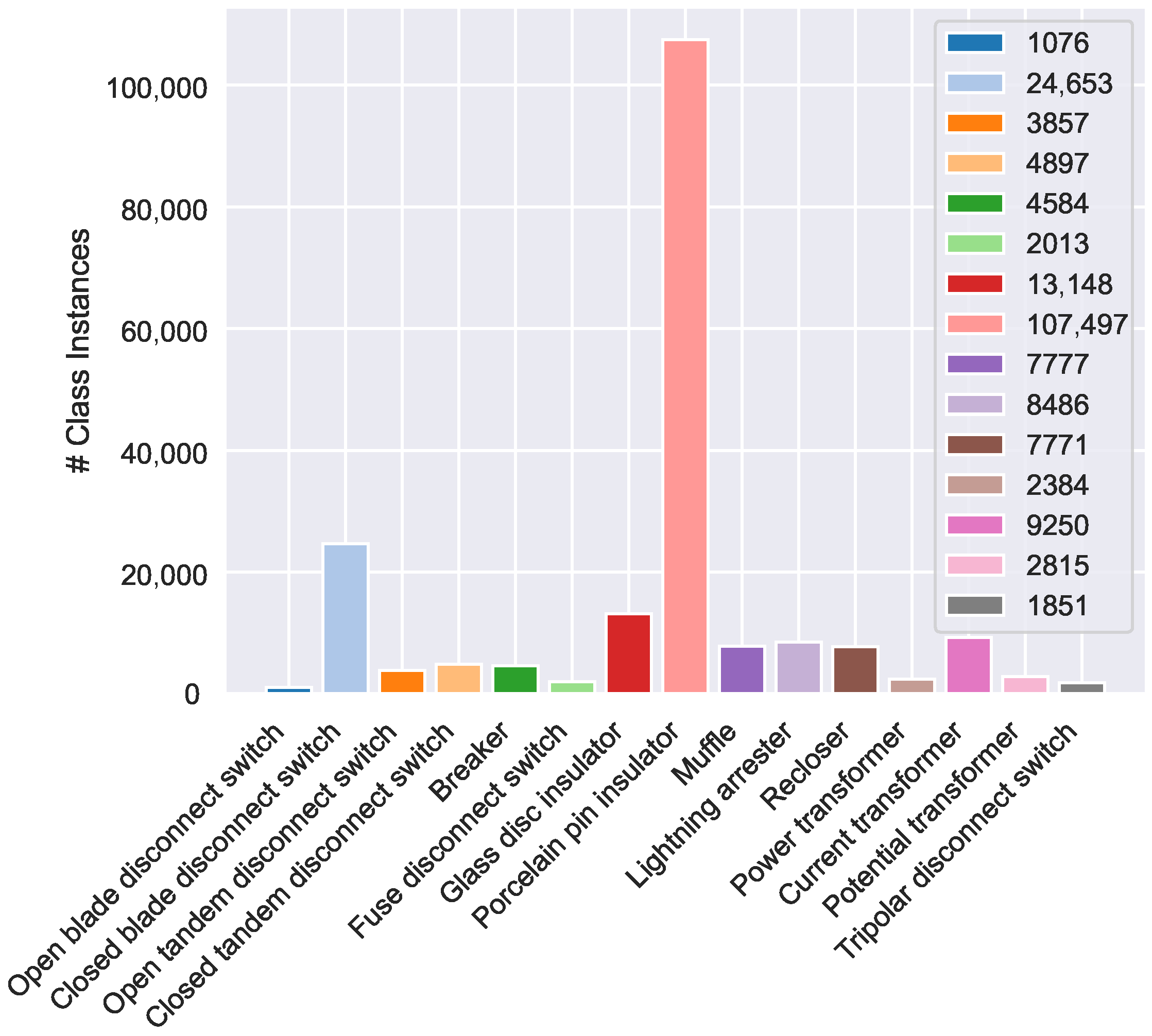
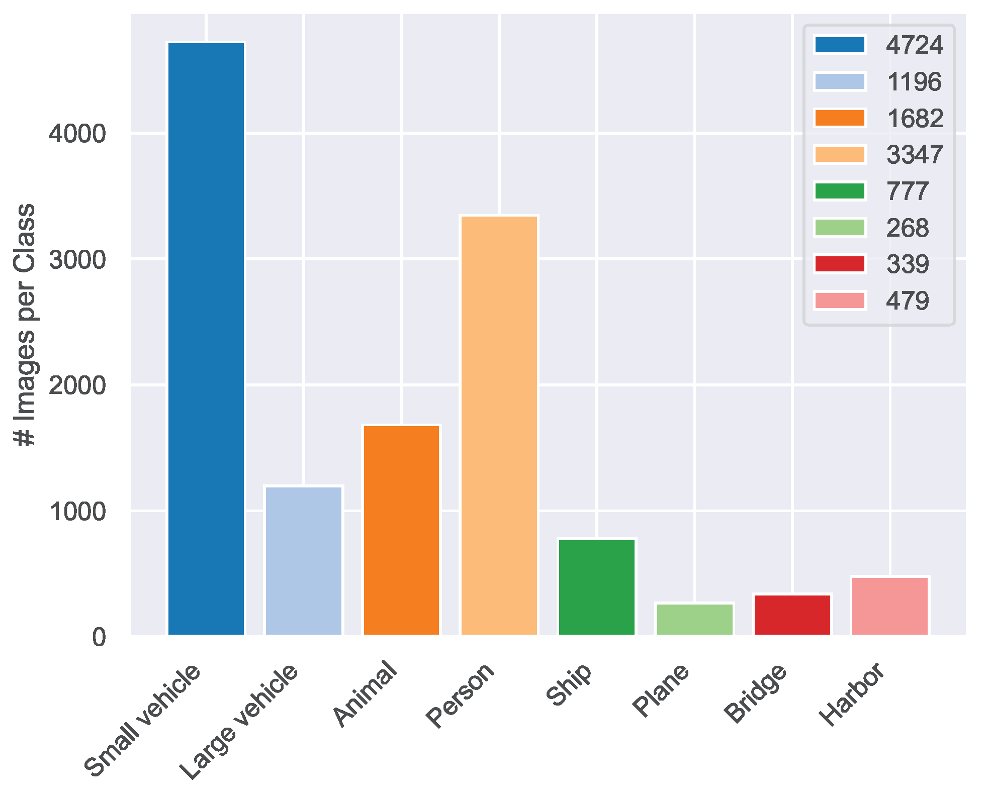
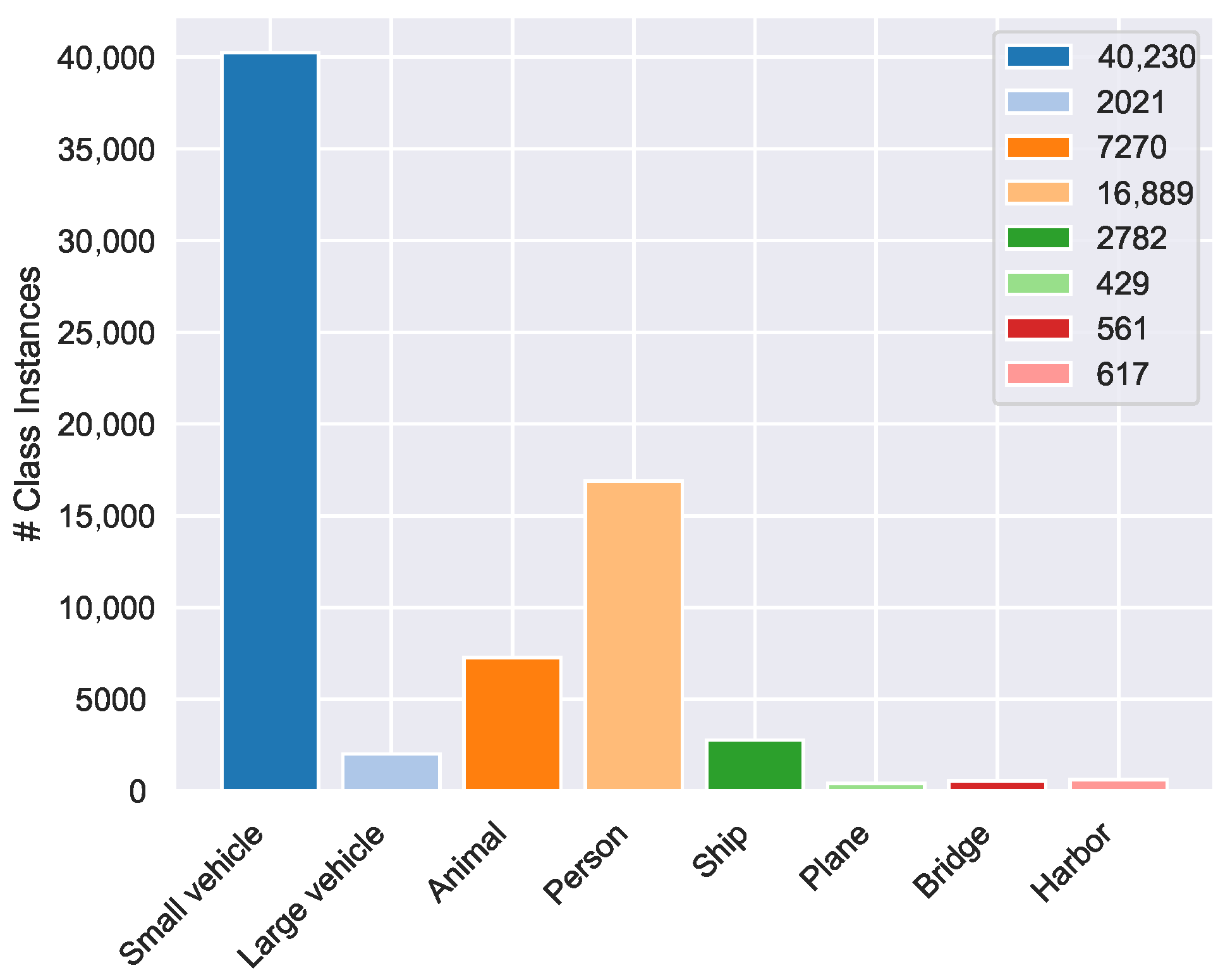
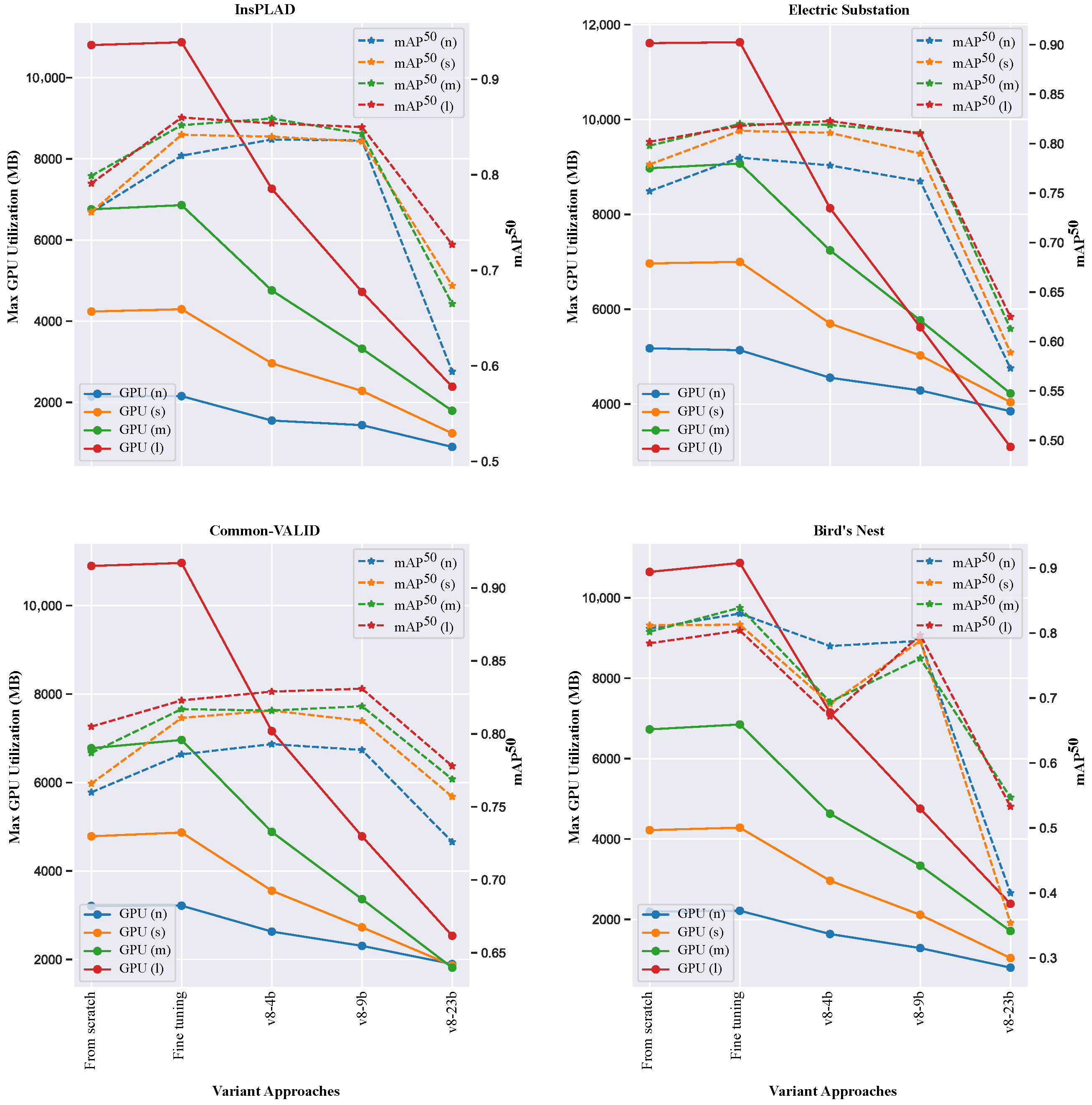
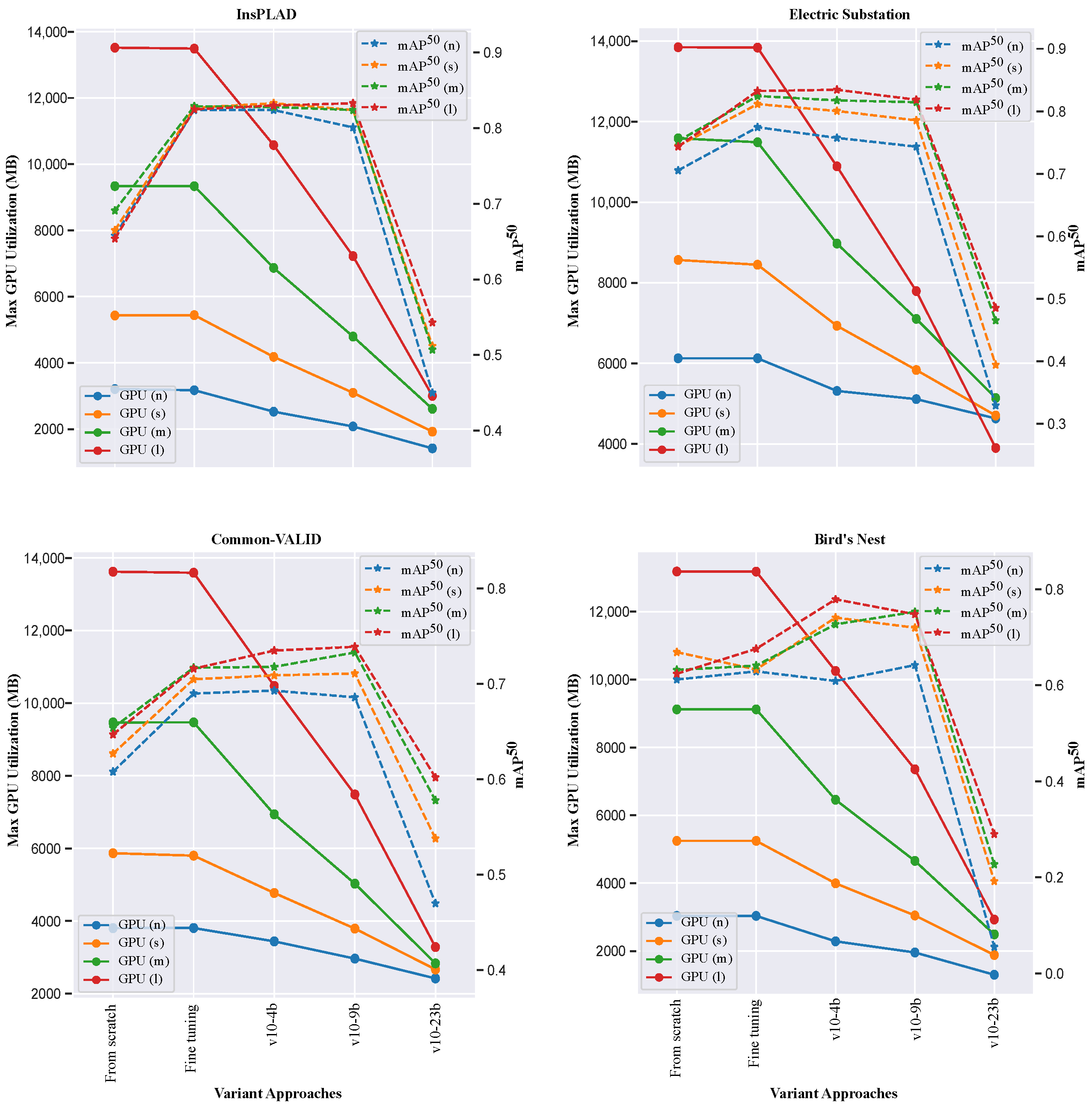
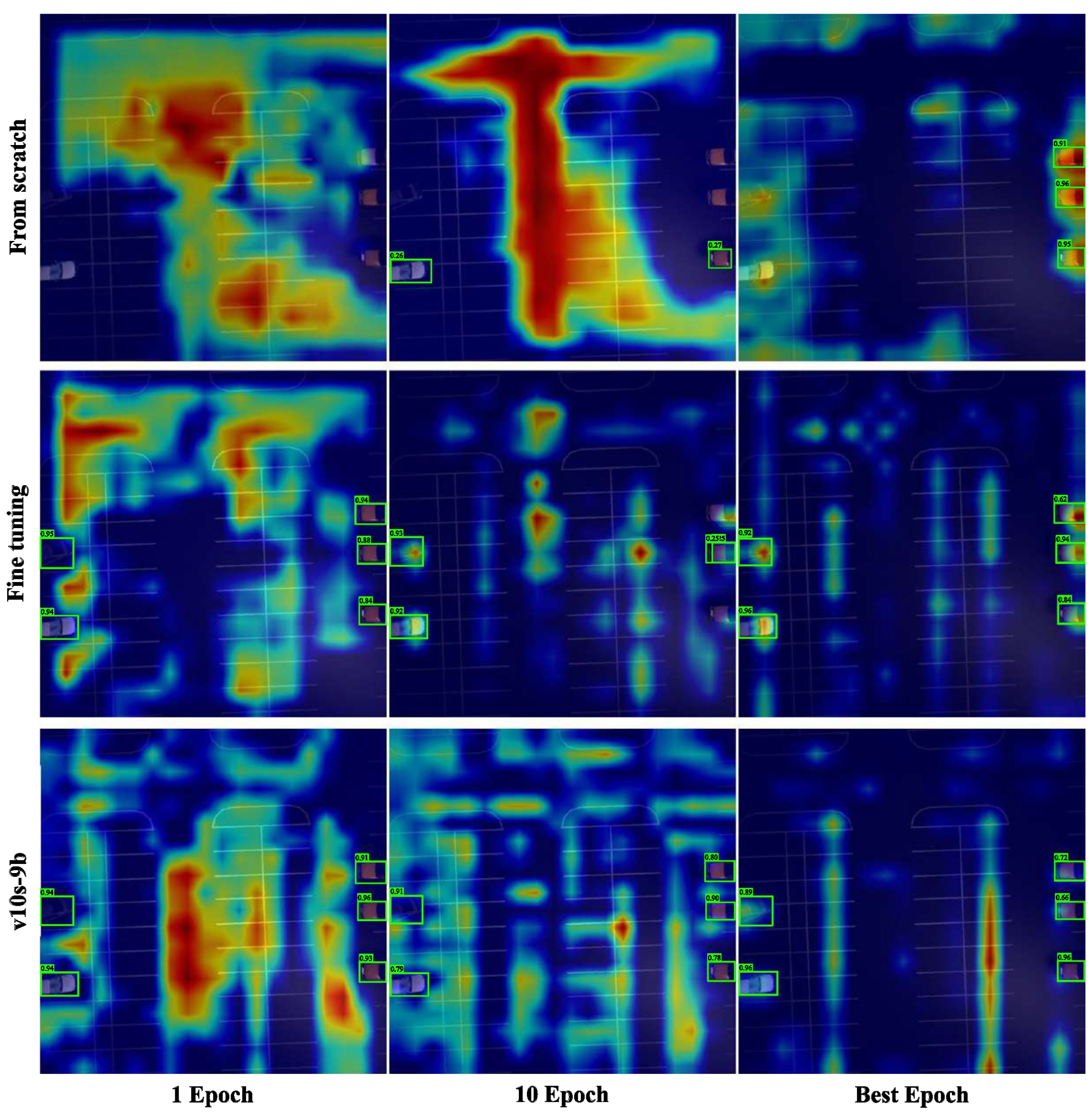
This section details the experimental methodology employed to systematically evaluate the impact of transfer learning strategies, particularly layer freezing, on the performance and computational efficiency of YOLOv8 and YOLOv10 models. Our general strategy involves two main components. We implement and compare several layer freezing configurations, where specific blocks of the pre-trained models’ backbones are frozen during retraining on target datasets. These configurations, corresponding to freezing the initial 4 blocks (FR1), 9 blocks (FR2, encompassing the backbone), or 22/23 blocks (FR3) are benchmarked against standard fine-tuning and training from scratch. The evaluation across all experiments relies on key performance metrics (mAP@50, mAP@50:95) and resource indicators (GPU usage, training time), as described below.
5.1. Layer Freezing and Implementation Details
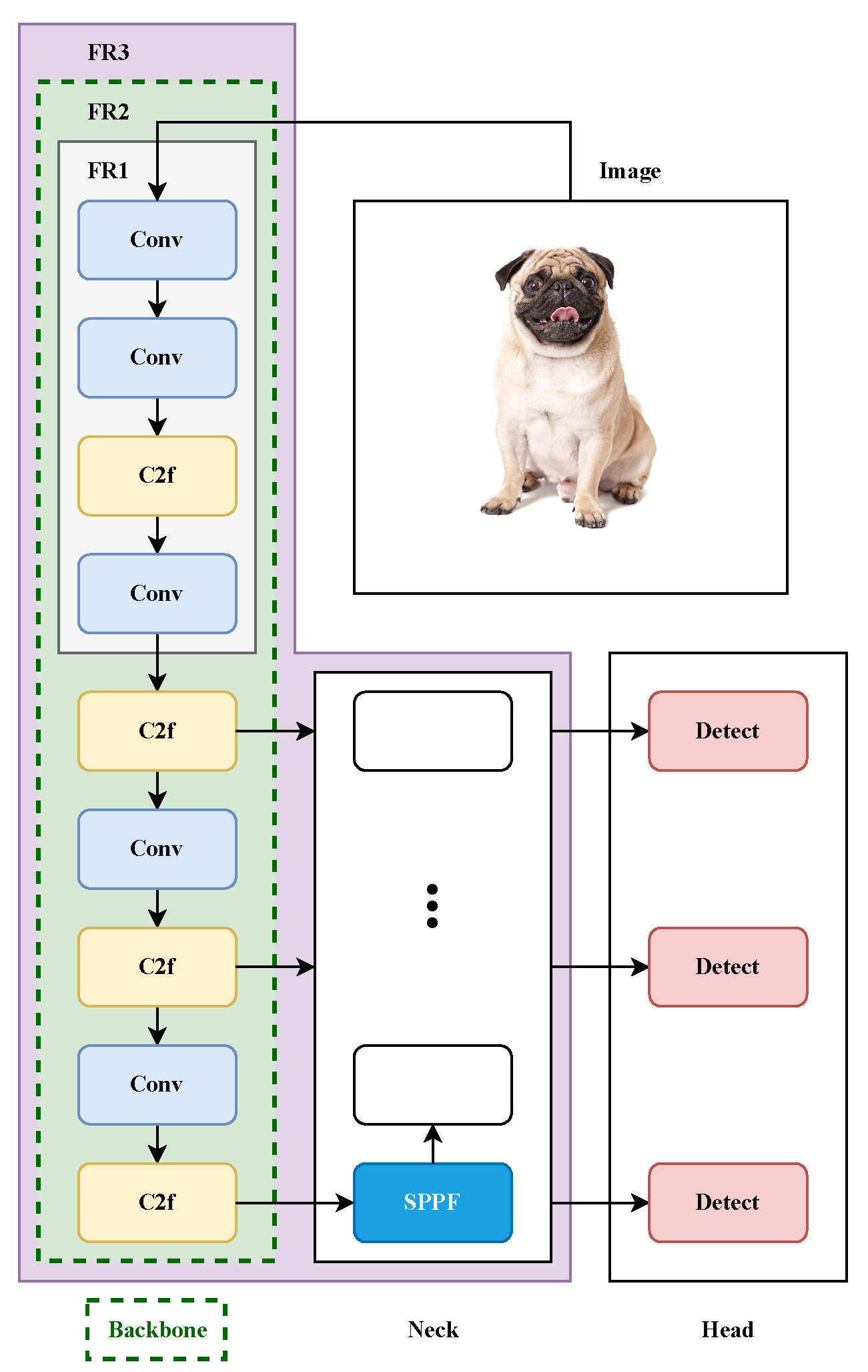
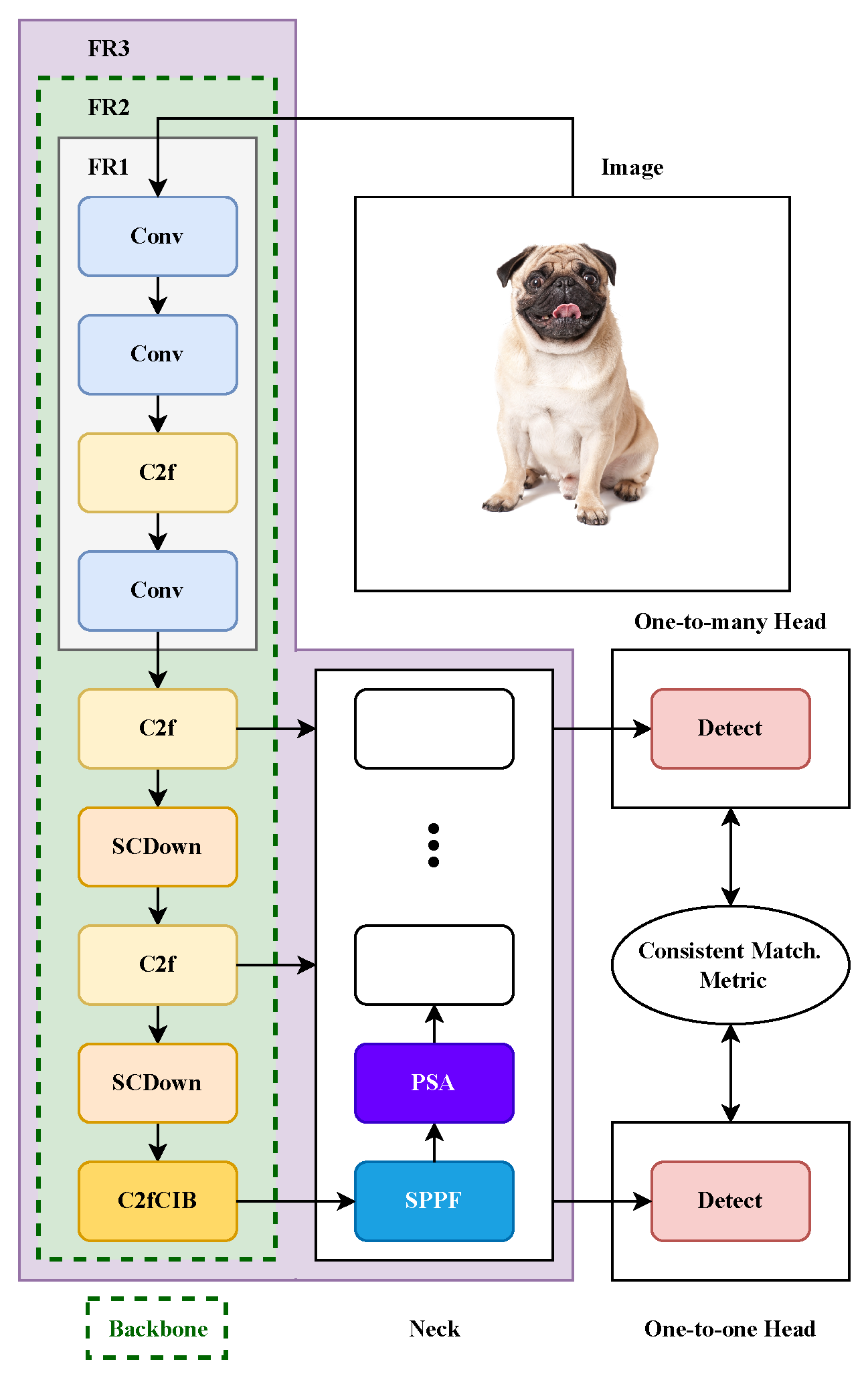
For our experiments, we will base the layer-freezing approach on the architectural details of the YOLO models under investigation (see
Figure 1 and
Figure 2) and the percentage of parameters frozen. It is important to note that this number of parameters includes the cv2 and cv3 modules for YOLOv10, as the original paper introducing YOLOv10 does not include these parameters in Table 1 [
13] since they are not needed during inference.
With regard to the parameters, the number of trainable parameters in the architecture’s heads may vary, depending on the different number of object classes in the datasets discussed in
Section 4. We will present the percentage of frozen parameters for each approach, model, and dataset, relative to the architecture of models pre-trained on the COCO [
7] dataset, which includes 80 object classes, and including cv2 and cv3 modules for YOLOv10. However, the difference in the number of parameters between a model with 80 object classes and one with a single class is less than 0.3%.
Table 4 shows the percentage of frozen parameters for each approach and model. “v8n-4b”, “v8n-9b”, and “v8n-22b” represent different approaches for the YOLOv8 model with variant “n” (nano), where “4b”, “9b”, and “22b” indicate the number of blocks frozen. Similarly, “v8s-4b”, “v8s-9b”, and “v8s-22b” refer to the “s” (small) variant of YOLOv8 with 4, 9, and 22 blocks frozen, respectively, and so forth for “m” (medium) and “l” (large) variants. The same structure is followed for the YOLOv10 model. These approaches involve freezing the layers enclosed in the areas labeled FR1, FR2, and FR3, as shown in
Figure 1 and
Figure 2. Specifically, the FR1 regions correspond to freezing 4 blocks, the FR2 regions correspond to freezing 9 blocks, and the FR3 regions correspond to freezing 22 or 23 blocks for YOLOv8 and YOLOv10, respectively. For additional information on the selection of blocks to freeze, please refer to
Appendix A.
Our selection of freezing configurations (FR1: 4 blocks; FR2: 9 blocks; FR3: 22/23 blocks) is grounded in the fundamental architectural boundaries of modern YOLO designs. Blocks 0–3 (FR1) constitute pure feature extraction layers positioned before any concatenation operations, capturing domain-agnostic visual representations (edges, textures, geometric patterns) with high transferability across detection tasks. The 9-block boundary (FR2) encompasses the complete backbone feature extraction pipeline, preserving all fundamental visual representations while allowing task-specific adaptation in the neck and head components. The extended 22/23-block configuration (FR3) includes most feature fusion operations, maintaining both feature extraction and integration capabilities while enabling fine-tuning only in the final detection layers. This hierarchical approach aligns with established transfer learning principles: early layers contain universal features suitable for preservation, intermediate layers handle feature integration requiring moderate adaptation, and final layers perform task-specific detection requiring full fine-tuning [
5].
By selectively freezing the backbone blocks and layers in both YOLOv8 and YOLOv10 models, we aim to preserve the general feature extraction capabilities learned from the original dataset while allowing the upper layers to adapt to the specific characteristics of the new task. This approach will help us determine the optimal layers and blocks to freeze.
In our experiments, YOLOv8 and YOLOv10 models are trained using the stochastic gradient descent (SGD) optimizer for 1000 epochs, with an early stopping mechanism employing a patience of 30 epochs. The batch size is set to 16, and dataset images are cached in RAM to enhance training speed by minimizing disk I/O operations, which comes at the cost of increased memory usage. The momentum and weight decay for the SGD optimizer are configured to 0.937 and , respectively. The initial learning rate is set to , decaying linearly to over the course of training. All dataset images underwent standardized preprocessing to ensure consistency across experiments while preserving data distribution integrity. Images were resized to 640 × 640 pixels and normalized using ImageNet statistics (mean: [0.485, 0.456, 0.406]; standard deviation: [0.229, 0.224, 0.225]). We intentionally avoid applying data augmentation techniques during the training process to prevent introducing any stochastic shifts in the original distribution of the datasets, which could potentially affect the validity and reliability of our experimental results.
Additional hyperparameters include a warm-up phase consisting of three epochs, with a warm-up momentum of 0.8 and a warm-up bias learning rate of 0.1. The learning rate schedule follows a linear decay pattern. The specific loss gains are set as follows: the box loss gain is 7.5, the class loss gain is 0.5, and the dual focal loss gain is 1.5.
To ensure a fair comparison between architectures, all experiments for both YOLOv8 and YOLOv10 were conducted using the same hardware setup, an NVIDIA RTX A4000 GPU with 16 GB of memory. This unified configuration eliminates hardware-induced bias in training time and GPU memory usage metrics, enabling a direct and reliable comparison between the two architectures.
A comprehensive summary of the experimental environment and training hyperparameters is provided in
Table 5.
5.2. Gradient Monitoring, Visual Analysis, and Metrics
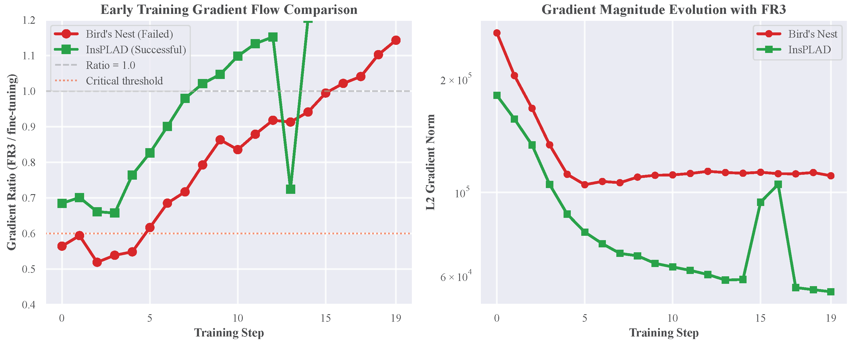
To gain deeper insights into the training dynamics and convergence behavior of different layer freezing strategies, we implement comprehensive gradient monitoring and visual analysis techniques. We aim to deepen the comprehension of one of the fundamental aspects of the proper convergence of the models during its training, the gradients. Concretely, the gradients of the model parameters with respect to the input. The formal definition of these parameters is as follows:
where
are the model parameters,
is the loss function,
x is the input, and
y is the target output.
For the monitoring of the gradients during training, we have decided to focus on their magnitudes using L2 Norm, defined as follows:
The L2 norm provides a scalar value representing the overall magnitude of the gradients for each layer or the entire model. By tracking the L2 norm over training iterations, we can gain insights into the training dynamics and identify potential issues. To visualize the L2 norm of gradients, we compute it at the end of each training batch.
The process begins by initializing a variable to accumulate the squared magnitudes of the gradients. For each parameter in the model, we check whether the gradient is available. If it is, we calculate the L2 norm of that gradient, square it, and add it to our accumulation variable. Once all parameters are processed, we take the square root of the accumulated value to obtain the L2 norm for that specific batch. This value is then stored in a list that tracks the L2 norms across all batches.
After the training process is completed for a specific epoch, we compute the mean of the L2 norms across all batches, excluding instances where the norm is zero to avoid skewing the average. This process provides a single representative value that reflects the overall gradient behavior during training. By using this approach, we can effectively monitor the gradients and assess the convergence of the model.
To complement the gradient magnitude analysis and provide visual understanding of model focus during training, we implement a gradient-weighted class activation mapping (GradCAM) analysis. This technique enables us to visualize which regions of the input images the model prioritizes during the detection process under different layer-freezing strategies.
The GradCAM methodology works by weighting the 2D activations by the average gradient, thereby generating visual explanations that highlight the key objects and regions that influence the model’s predictions. For our YOLO architectures, we compute activation maps using the implementation provided by [
32], which is specifically adapted for object detection models.
The GradCAM computation process involves several steps: first, we extract feature maps from a target convolutional layer within the model; second, we compute the gradients of the class score with respect to these feature maps; third, we pool the gradients across the width and height dimensions to obtain the neuron importance weights; and finally, we perform a weighted combination of the forward activation maps and apply a ReLU function to focus on features that have a positive influence on the class of interest.
This visual analysis methodology allows us to track how the model’s attention evolves across training epochs and how different layer-freezing strategies affect the focus patterns. By generating activation maps at key training milestones (epoch 1, epoch 10, and the epoch with the best validation loss), we can observe the adaptation process and validate whether the models are learning to focus on relevant object features during the transfer learning process.
To thoroughly evaluate the performance of the YOLO models under different training strategies, we will focus on two key metrics: mAP@50 and mAP@50:95. These metrics provide a comprehensive assessment of the models accuracy and precision, with mAP@50 measuring the mean average precision at a 50% intersection over union (IoU) threshold and mAP@50:95 offering a more detailed evaluation across a range of IoU thresholds from 50% to 95%.
For the validation over the test and validation/test splits, we will use a minimum confidence threshold of 0.5. This setting ensures that only detections with a confidence level above 50% are considered, effectively discarding less certain detections and reducing the likelihood of false positives.
Additionally, we will apply an IoU threshold of 0.7 for non-maximum suppression (NMS) during the validation of YOLOv8 models. This threshold helps in reducing duplicate detections by suppressing overlapping bounding boxes, thereby improving the quality of the detected objects. It is important to note that IoU-based NMS is only applicable to YOLOv8, as YOLOv10 employs a free-NMS approach, which does not require a predefined IoU threshold for suppressing redundant detections.
By comparing the mAP@50 and mAP@50:95 values for different training strategies, including layer freezing, fine-tuning, and training from scratch, we can gain insights into the models’ performance and the effectiveness of each approach in terms of accuracy and precision. Additionally, we will measure the training time and GPU usage for each case to assess the computational efficiency. The training time will be recorded in minutes, and GPU usage will be monitored using a tool like NVIDIA System Management Interface (nvidia-smi) to track the GPU memory consumption and utilization during the training process. The combination of accuracy metrics (mAP@50 and mAP@50:95) and computational efficiency metrics (training time and GPU usage) will provide a comprehensive evaluation of the YOLO models under different training strategies, enabling us to identify the most effective approach for balancing accuracy and computational resources.

