1. Introduction
Automated quality control has become an essential component in modern industries, especially in environments that handle large volumes of packaged products requiring fast, consistent, and accurate inspections [
1].
Ensuring product integrity is not only crucial to meet customer expectations and standards but also helps reduce waste, minimize returns, and maintain high operational efficiency. For example, Winkelbauer demonstrates how artificial intelligence applied to manufacturing can optimize production parameters and significantly reduce waste generation [
2]. Similarly, a case study presented at the Sustainable Manufacturing Expo showed that the implementation of automated quality control systems enabled an automotive manufacturer to decrease material waste by 47% in just six months.
In recent years, CNNs have emerged as essential tools in industrial visual inspection systems, enabling automatic extraction of features from images without manual engineering. Real-time defect recognition on steel surfaces using CNNs has proven effective in accelerating industrial workflows [
3]. Comprehensive reviews confirm their robustness and applicability across a wide range of industrial scenarios [
4]. Additionally, lightweight CNN-based methods have been developed specifically for defect detection on metal surfaces, balancing accuracy and computational efficiency [
5].
Furthermore, in related fields such as biomedicine, CNNs have also demonstrated their versatility for automatic diagnostic tasks with proven success [
6]. These advances complement and strengthen the confidence in the use of CNNs in complex industrial applications.
When defective data is limited or difficult to label, significant challenges arise for the effective training of CNNs, as their performance typically depends on balanced and well-representative datasets [
7]. For this reason, the combination of CNNs with OCC methods has been explored as a promising alternative to detect anomalies based solely on normal examples, favoring practical applications in industrial environments with scarce fault data.
To overcome the limitations of traditional supervised methods like CNNs in scenarios with scarce or imbalanced defective data, OCC methods have gained popularity, especially in anomaly detection tasks [
7]. These models are trained exclusively with normal data and are designed to identify deviations or atypical patterns in new samples. This approach is especially useful when defective samples are scarce, highly variable, or unknown, enabling the detection of previously unseen anomalies [
8].
Among the most representative methods in this area are the OCSVM, which defines a hyperplane to separate most of the normal data from the origin [
9]; the Isolation Forest (IF), which isolates observations by random partitioning of the feature space [
10]; the Local Outlier Factor (LOF), which evaluates the local density of each point and detects anomalies based on density differences with respect to its neighbors [
11]; the Elliptic Envelope (EE), which estimates a robust elliptical envelope based on a Gaussian distribution to delimit the space considered normal [
12]; Autoencoders, which use neural networks to reconstruct inputs and detect anomalies when reconstruction errors are high [
13]; and the SVDD, which constructs a minimum hypersphere enclosing the normal data and allows the identification of significant deviations [
14].
Besides selecting suitable models for anomaly detection, it is essential to apply strategies that improve their generalization capability and adaptability to the variable conditions of industrial environments. Among these strategies, data augmentation has proven particularly useful, as it allows us to expand the training set through transformations such as rotations, scaling, or brightness changes, without the need to collect new samples [
15,
16].
On the other hand, hyperparameter optimization using techniques such as GridSearchCV, Bayesian optimization, or evolutionary algorithms also significantly contributes to model performance [
17]. The combination of these strategies reinforces the robustness of deep learning-based automatic inspection systems.
1.1. Objective
This study aims to develop an automated anomaly detection system for the inspection of candle jars, a common product in the packaging industry that presents particular challenges due to the variety of possible defects, such as broken jars or stains. Given the practical limitations of traditional inspection methods in this context, a computer vision-based solution is especially suitable.
To address this problem, two complementary defect detection approaches are explored:
Direct CNN Classification: A CNN is trained using images of both normal and defective jars. The CNN is employed for both automatic feature extraction and final classification. This approach specifically analyzes the model’s ability to discriminate between normal and defective jars while varying the proportion of defective samples in the training set. This evaluation allows us to assess the robustness of the model under class imbalance scenarios, a common condition in industrial environments. The results indicate the extent to which the CNN can maintain adequate performance even with scarce defective examples.
Hybrid Model: CNN + OCC: In this approach, features are first extracted by a CNN trained on normal images and a very limited percentage of defective ones. These representations are then used as input for OCC algorithms, which are primarily trained on normal class data. This method is especially suitable in contexts where defects are infrequent, as it allows precise modeling of the normal class distribution and detection of deviations without requiring many negative examples.
Due to the limited number of defective samples, data augmentation is applied specifically to the affected classes to compensate for imbalances and enhance the model’s generalization ability. This process artificially increases the training dataset and simulates the natural variability of the production environment without requiring additional real samples.
Moreover, advanced feature selection and hyperparameter optimization techniques are implemented to enhance system performance. Methods such as GridSearchCV, RandomizedSearchCV, Bayesian optimization, and genetic algorithms are employed, enabling efficient exploration of the parameter space and appropriate configuration selection to maximize defect detection.
1.2. Key Contributions
The key contributions are as follows:
Development of a hybrid inspection system combining CNN-based feature extraction with One-Class classification models for robust anomaly detection.
Utilization of a very limited number of defective samples, reflecting realistic industrial scenarios.
Application of targeted data augmentation on defective images to address data imbalance and improve model generalization.
Implementation of advanced hyperparameter optimization and feature selection algorithms (e.g., Bayesian optimization and genetic algorithms) to maximize detection performance.
Proposal of a practical solution designed for real-world deployment in the packaging industry, particularly for candle jar inspection.
To achieve the goals of this research, the structure of the paper is as follows: In
Section 2, the CNN and OCC models are presented, along with their theoretical basis and relevance for detection-related tasks.
Section 3 describes the dataset, the preprocessing process, and the methodology used for feature extraction and classification.
Section 4,
Section 5,
Section 6 and
Section 7 detail the training and evaluation strategy, discuss the experimental findings, and conclude the study.
2. Machine Learning
Machine Learning (ML) is a pivotal branch of artificial intelligence that focuses on the development of algorithms and models capable of learning from data to improve their performance autonomously, without explicit programming. ML methodologies are broadly categorized into supervised, unsupervised, and semi-supervised learning paradigms [
18,
19]. This work emphasizes both supervised and unsupervised approaches, deploying them at different stages within our methodology.
2.1. Supervised Learning: CNNs
CNNs represent a specialized class of deep learning architectures optimized for image processing tasks. Unlike unsupervised methods such as the OCSVM, CNNs are primarily trained through supervised learning using labeled datasets [
20]. Their ability to perform classification, segmentation, and feature extraction with high accuracy makes them indispensable in industrial image analysis.
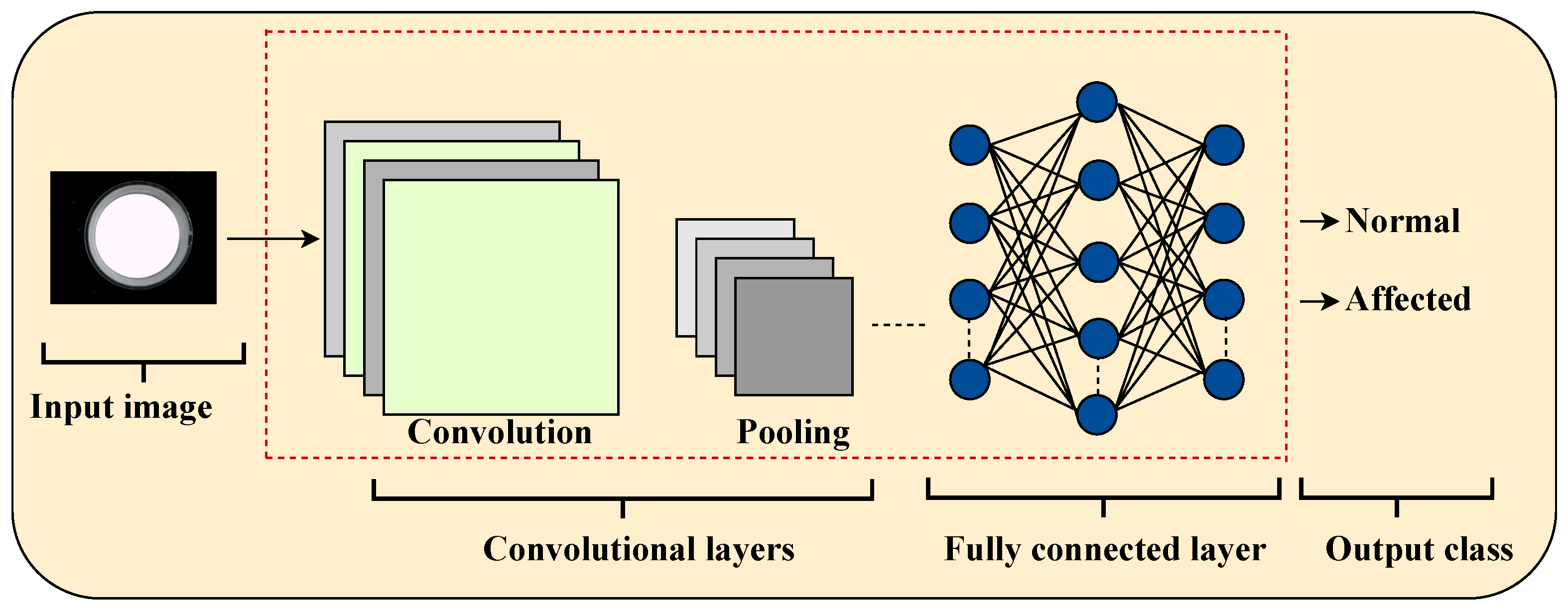
As illustrated in
Figure 1, CNNs consist of sequential layers that progressively transform raw images into predictive outputs. Each layer plays a specific role in capturing spatial and hierarchical features:
Input layer: It receives raw data from industrial images.
Convolutional layers: They use filters (kernels) to extract local features such as edges, textures, and shapes.
Activation functions (e.g., ReLU): They introduce non-linearity to enable learning of complex representations.
Pooling layers, such as max pooling: They reduce the dimensionality of feature maps while preserving the most relevant ones.
Fully connected layers: They integrate features to perform classification based on the learned representations.
Output layer: It generates final predictions using functions such as softmax or sigmoid, for example, to classify images as “Defective” or “Non-defective”.
Figure 1.
Typical CNN architecture illustrating the data flow from the input image to output classification.
Figure 1.
Typical CNN architecture illustrating the data flow from the input image to output classification.
2.2. Unsupervised Learning: Alternative Anomaly Detection Methods
Unsupervised learning methods are designed to uncover hidden structures or patterns in data without requiring labeled inputs. In the context of anomaly detection, these approaches are particularly valuable when labeled defective samples are limited or entirely unavailable. Several established algorithms are employed for this task [
21]:
OCSVM: It defines a decision boundary that encloses the majority of normal instances in the feature space, allowing outliers to be identified as deviations [
21,
22].
OCIF: It utilizes randomly generated decision trees to partition the dataset. Anomalies, being easier to isolate, tend to require fewer splits, making them distinguishable [
23,
24].
OCLOF: It evaluates the local density of data points and flags instances with significantly lower densities than their neighbors as potential anomalies [
25,
26].
OCAutoencoders: They are deep neural architectures trained to replicate their input at the output. Samples with high reconstruction errors are flagged as anomalous, indicating poor representation within the learned data distribution [
27].
OCEE: It assumes a multivariate Gaussian distribution and fits an elliptical boundary around the dataset. Points falling outside this boundary, measured via the Mahalanobis distance, are classified as outliers [
28].
Deep SVDD: It builds upon the SVDD framework by leveraging deep neural networks to learn compact, centralized representations of normal data, enabling more effective separation of anomalies in complex feature spaces [
29].
2.2.1. OCSVM
The OCSVM is a well-established unsupervised learning algorithm designed to identify anomalies by learning a decision boundary that encapsulates the majority of the normal data. It operates by projecting the data into a high-dimensional feature space using a kernel function and finding the hyperplane that best separates the origin from the mapped data with the maximum margin.
A training set consisting only of normal samples is defined as
and The kernel-induced feature map is given by
where
is a high-dimensional Hilbert space.
The optimization objective is to solve the following convex optimization problem (Equation (
3)):
subject to the constraints (Equation (
4)):
where
is the normal vector to the separating hyperplane;
is the offset;
are slack variables allowing for soft margin violations;
controls the trade-off between the fraction of outliers and the margin.
Once trained, the decision function used to classify new instances is expressed as (Equation (
5))
A sample
x is classified as anomalous if it satisfies the following condition (Equation (
6)):
2.2.2. OCIF
Isolation Forest is an unsupervised anomaly detection algorithm that isolates observations by randomly selecting features and split values. Unlike density- or distance-based approaches, iForest detects anomalies by leveraging the fact that they are more susceptible to isolation, typically requiring fewer splits in the tree-building process.
Input: A dataset of unlabeled instances is defined as
Training Procedure: An ensemble of t binary isolation trees is constructed by
Scoring Function: The anomaly score for a data point
x is computed as follows (Equation (
8)):
where
2.2.3. OCEE
The OCEE is a statistical anomaly detection method based on the assumption that normal data follow a multivariate Gaussian distribution. It fits an ellipse around the central data points using robust estimates of the mean and covariance matrix, identifying outliers as observations lying far outside this region.
Input: A set of
n multivariate observations is defined as
Training Procedure: Estimate the robust location and covariance of the data using
where typically the minimum covariance determinant (MCD) estimator is employed.
Scoring Function: Compute the squared Mahalanobis distance for each point
x (Equation (
13)):
Decision Rule: Let
denote the quantile of the chi-squared distribution with
d degrees of freedom at confidence level
. The anomaly decision is
2.2.4. OCAutoencoders
Autoencoders are neural network architectures designed to learn efficient representations of data through unsupervised learning. They consist of two main components: an encoder that compresses the input into a latent representation and a decoder that reconstructs the original input from this representation. Anomalies are identified based on high reconstruction error, under the assumption that the model reconstructs normal data well but fails on abnormal patterns.
Input: A set of input vectors is defined as shown in Equation (
16):
Architecture: The encoder compresses each input
into a latent vector
as defined in Equation (
17), where the latent dimension
k is smaller than the input dimension
d. The decoder reconstructs the input from the latent representation as described in Equation (
18):
Training Objective: The model is trained by minimizing the reconstruction loss shown in Equation (
19), which measures the average squared error between the input and its reconstruction:
Anomaly Scoring: For a new sample
x, the reconstruction error
is computed as shown in Equation (
20):
Decision Rule: A sample is classified as an anomaly if its reconstruction error exceeds a threshold
, as stated in Equation (
21). Otherwise, it is considered normal:
where
is a predefined or data-driven threshold based on the distribution of reconstruction errors on the training data.
2.2.5. SVDD
Support Vector Data Description (SVDD) is a kernel-based anomaly detection method that defines a minimal hypersphere in a high-dimensional feature space to enclose normal data. It is conceptually similar to the OCSVM but focuses on compactly enclosing the data rather than separating it from the origin.
A set of input vectors is given by Equation (
22):
Objective Function: The goal is to find the smallest hypersphere with center
a and radius
R that encloses the mapped data
in a reproducing kernel Hilbert space (RKHS). The optimization problem is defined in Equation (
23) and constrained as shown in Equation (
24):
Here,
is a kernel-induced map, and
is a regularization parameter that controls the trade-off between the volume of the hypersphere and tolerance to outliers.
Scoring Function: For a new sample
x, its squared distance to the center
a in the feature space is computed as shown in Equation (
25):
Decision Rule: The classification is based on the distance compared to the learned radius
R, as shown in Equation (
26):
2.2.6. OCLOF
OCLOF is an unsupervised anomaly detection method that evaluates the degree to which a data point is isolated based on the local density of its neighborhood. Anomalous points exhibit significantly lower density compared to their neighbors.
The input dataset is defined in Equation (
27):
Definitions:
LOF Score: The Local Outlier Factor of point
x is defined in Equation (
30):
Interpretation:
: x has similar density to its neighbors (normal).
: x is in a lower-density region (potential anomaly).
: x has strong anomaly indication.
Decision Rule: As shown in Equation (
31), a sample is flagged as anomalous if
where
is a threshold selected based on validation data or statistical analysis.
2.3. Hyperparameter Optimization Methods
To enhance the performance and reliability of the anomaly detection models, we applied four different hyperparameter optimization techniques. This systematic tuning allowed for effective adaptation of each algorithm to the extracted features and improved detection accuracy. The typical parameter ranges used for each algorithm are summarized in
Table 1.
3. Materials and Methodology
This study proposes a hybrid approach for the detection of defective products in industrial manufacturing processes, combining CNNs for automatic feature extraction with OCC algorithms for anomaly detection.
The following subsections describe in detail the training and evaluation phases of the proposed model, including data preparation and augmentation, feature extraction, classifier optimization, and performance validation on unseen samples.
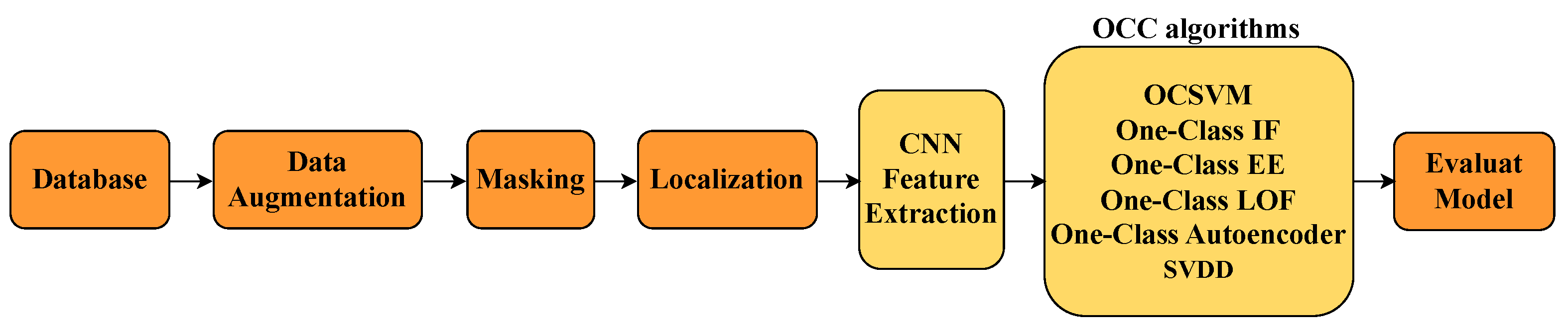
3.1. Training Process
The training phase was divided into several stages, as illustrated in
Figure 2.
3.1.1. Stage 1: Dataset Preparation
Images were categorized into two groups: normal products and defective products.
To train the CNN as a feature extractor, a dataset consisting primarily of normal images was used, supplemented by approximately 5% of the available defective samples.
The remaining 95% of defective images were reserved for the testing phase, where OCC algorithms were applied.
3.1.2. Stage 2: Data Augmentation
To address class imbalance and improve model generalization, data augmentation techniques such as rotation, translation, scaling, and adjustments to brightness and contrast were applied, primarily to 5% of the defective images used in training.
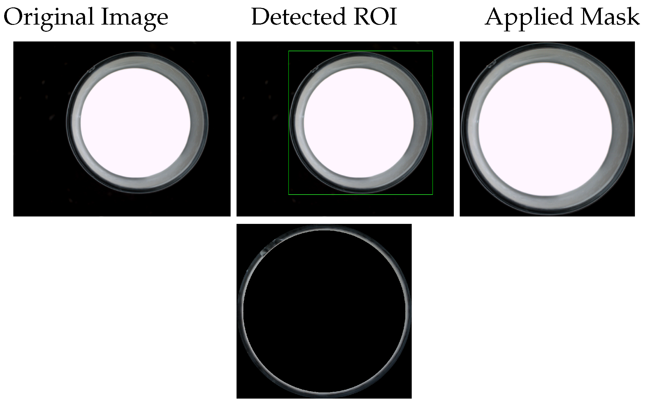
3.1.3. Stage 3: Preprocessing and ROI Extraction
Image enhancement techniques such as histogram equalization, normalization, and noise reduction were employed.
The region of interest was extracted using contour detection and binary masks to isolate the inspection object from the background.
3.1.4. Stage 4: Feature Extraction with the CNN
The CNN architecture was trained using the prepared dataset, consisting of 95% normal and 5% defective images, enabling the model to learn discriminative representations.
The features learned by the CNN were used as input vectors for the one-class classifiers.
3.1.5. Stage 5: Training One-Class Classifiers
3.1.6. Stage 6: Classifier Selection and Hyperparameter Optimization
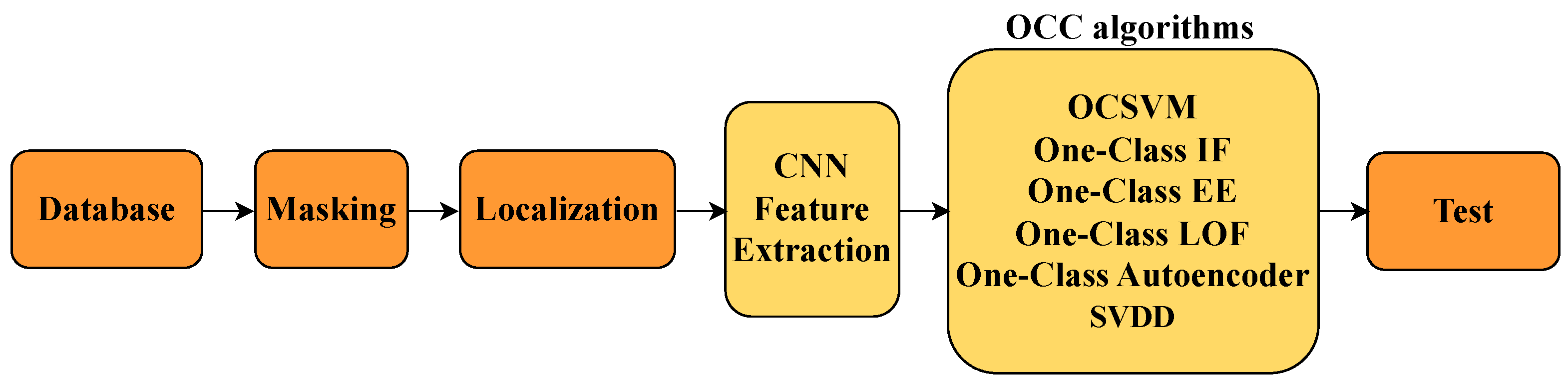
3.2. Evaluation Process (Testing Phase)
After completing the training phase, the system’s performance was evaluated using a test set composed of samples not seen during training. This stage serves to validate the model’s generalization ability and effectiveness under real-world conditions, as illustrated in
Figure 3.
3.2.1. Stage 1: Test Set Preprocessing
The test images underwent the same preprocessing steps as during training, including normalization, histogram equalization, and noise reduction.
The region of interest was extracted using binary masks and contour detection to isolate the candle jar.
3.2.2. Stage 2: Feature Extraction
3.2.3. Stage 3: Model Evaluation
The trained one-class classifiers were used to determine whether each sample belonged to the normal class or exhibited anomalies.
Metrics such as precision, recall, F1-score, and ROC-AUC were computed to compare the performance of the various models.
3.2.4. Stage 4: Visualization of Results
Visualization techniques were used to better understand model performance, including ROC curves, true versus predicted label distributions, and accuracy histograms.
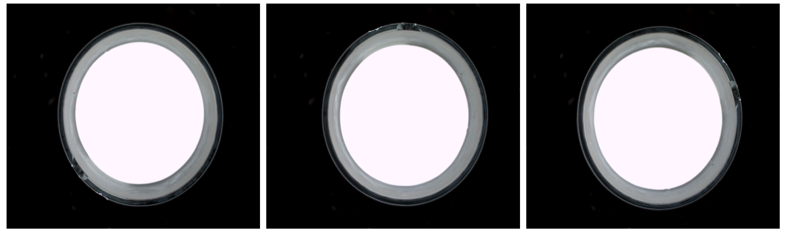
3.3. Dataset
The dataset used in this study was provided by the PYGSA (Valencia, Spain) company database. The images were captured directly from the production line under real-world conditions using a machine vision system with controlled lighting. Each image depicts a container with plastic cups, and the goal of the analysis is to classify their visual condition.
The images are categorized into two classes:
Normal: Cups without visible defects.
Defective: Cups that present visible issues, including glass breakage, structural cracks, stains, or other noticeable anomalies.
In total, 480 images of candle jars were collected, including both normal and defective samples. All images were resized to 150 × 150 × 3 pixels and normalized to the range [0, 1] before being used for model training and validation.
Figure 4 presents representative cropped regions from defective samples in the dataset. These highlight the visual variability of anomalies found in the inspection process, such as structural damage and contamination.
3.4. Preparing the Data and Preprocessing
3.4.1. Data Augmentation
Due to the limited size of the original dataset, data augmentation techniques were employed to increase both the diversity and the number of samples during training. This approach is essential in deep learning models, as it helps enhance generalization and mitigate overfitting.
After normalizing the images, simple geometric transformations were applied—primarily rotations in multiples of 30 degrees (i.e., n × 30°, where n = 0, 1, 2, …), with n representing the number of image augmentations. This strategy simulates various perspectives and positional variations that may occur in real production scenarios while preserving the structural integrity of the objects. The candle jars are generally centered or near the optical axis of the camera, making their mouths appear nearly circular in the images, which allows rotations up to 360° without introducing distortions.
Figure 5 illustrates examples of augmented images generated through rotation, based on the candle jar dataset.
3.4.2. ROI Localization
After capturing images of candle jars, a preprocessing stage is conducted to accurately locate the relevant region within each image. This step is essential to eliminate irrelevant background information and focus the analysis on the jar area.
To accomplish this, an edge detection algorithm is applied through three key steps to delineate the jar region precisely. This isolates the ROI before inputting it to the deep learning model.
Image Processing: Initially, basic transformations such as grayscale conversion, adaptive thresholding, and contour detection are performed. The contours are analyzed to compute the area and centroid of each object, and the bounding box enclosing the jar is identified. The jar region is then extracted from the original image.
Following ROI localization, further preprocessing such as scaling, noise reduction, and centering is applied to prepare the images for CNN analysis.
Figure 6 illustrates this workflow—from the original image to ROI extraction and mask application.
3.5. Feature Extraction with CNNs
The architecture of CNNs can be conceptually divided into two main functional blocks: (1) the feature extraction block and (2) the classification block. This division is essential to understand how the intermediate representations extracted from the network are utilized for downstream tasks, such as one-class model-based classification.
3.5.1. Feature Extraction Block
The convolutional and pooling layers are responsible for feature extraction. These layers learn hierarchical spatial patterns, starting from edges and textures to complex shapes that characterize the visual content.
The convolution operation between an input image
I and a filter
K is defined as
Subsequently, max pooling is applied to reduce the dimensionality of the activation maps:
These intermediate representations (activation vectors) are extracted from the layers prior to classification and used as visual descriptors for unsupervised OCC methods.
3.5.2. Classification Block
When the CNN is trained in a supervised manner, the generated feature vector is flattened and passed through fully connected layers, which perform the binary classification task. The output of the last dense layer is computed as
where
x represents the input vector,
W and
b are the learned weights and biases, and
is the sigmoid activation function.
Note: In our approach, the dense layers are used only during auxiliary supervised training. For feature-based classification (e.g., with OCSVM), these layers are discarded, retaining only the feature extractor.
Table 2 presents the architecture of the CNN used for feature extraction and auxiliary classification training.
4. Model Training and Evaluation
In this work, two deep learning-based classification approaches have been implemented for the analysis of candle vessel images: (1) a supervised CNN model trained directly as a binary classifier and (2) a set of unsupervised models that use representations extracted from the pretrained CNN as input feature vectors. To ensure robustness and reduce overfitting, 5-fold cross-validation was applied during model training and evaluation [
30].
To ensure consistent and fair evaluation, the dataset was partitioned differently for each approach, as detailed in the following subsections.
4.1. Supervised Classification with the CNN
In the supervised approach, the entire convolutional network (including the dense layers) is trained as a binary classifier. The dataset was split according to the following criteria:
Normal data: A total of 80% of the normal images were used for training, with the remaining 20% reserved for testing.
Affected data: Only 5% of the affected vessel images were included in the training set, applying data augmentation to balance the classes. The remaining 95% were kept for testing.
This training scheme with an imbalanced ratio aims to simulate a realistic scenario where anomalous samples are scarce. The test set includes a mixture of normal and affected data, allowing evaluation of the model’s ability to discriminate between both classes. During training, the binary cross-entropy loss function and the Adam optimizer were used. Performance metrics monitored included accuracy, precision, sensitivity, and the area under the ROC curve (AUC).
4.2. Unsupervised Classification with CNN Feature Vectors
This part of the study evaluates unsupervised classification methods based on feature vectors extracted using a CNN. Subsequently, OCC models are applied to detect anomalies and classify the samples.
In this approach, the CNN is used solely as a feature extractor, discarding the dense classification layers. Activation vectors are obtained from the penultimate layer (just before the output), representing each image as a point in a high-dimensional feature space.
The data split was organized as follows:
Unsupervised training: A total of 80% of the normal images (the same ones used in supervised training) were used to build the model.
Evaluation: The remaining 20% of the normal images and 95% of the affected images were used to assess classifier performance. It is important to note that these evaluation images were not used during CNN training, ensuring an unbiased assessment of the unsupervised model.
These techniques are particularly useful in industrial contexts where anomalous samples are very scarce or unknown during training. Evaluation metrics are similar to the supervised approach, with particular emphasis on sensitivity and the false alarm rate.
4.3. Performance Metrics
The performance of the evaluated models—both the supervised CNN and unsupervised OCC—was measured using a standard set of metrics widely adopted in binary classification tasks. The metrics considered include overall accuracy, recall (sensitivity), precision, the F1-score, and the area under the ROC curve [
31].
The AUC value is obtained from the ROC (receiver operating characteristic) curve, which depicts the trade-off between the true positive rate (TPR) and the false positive rate (FPR). A higher AUC value indicates better discriminative capability of the model between normal and affected classes.
In addition, precision–recall curves (PRCs) were analyzed as another evaluation parameter, as they are especially relevant for datasets with class imbalance. PRCs emphasize the trade-off between precision and recall, providing a more informative measure of performance when the positive class (affected cases) is rare.
5. Results
This section presents the results obtained from the various classifiers, both supervised and unsupervised, applied to the task of detecting affected candle vessels.
To improve performance, hyperparameter optimization was conducted on those algorithms that allowed it.
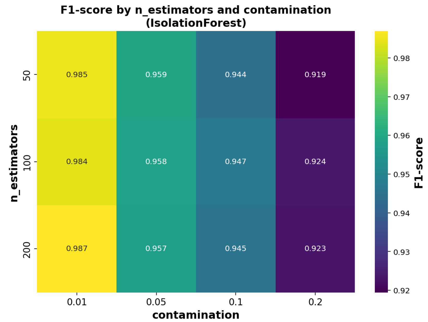
For the OCIF model, the performance was analyzed by varying the number of estimators (_estimators) in relation to the contamination parameter, as presented in
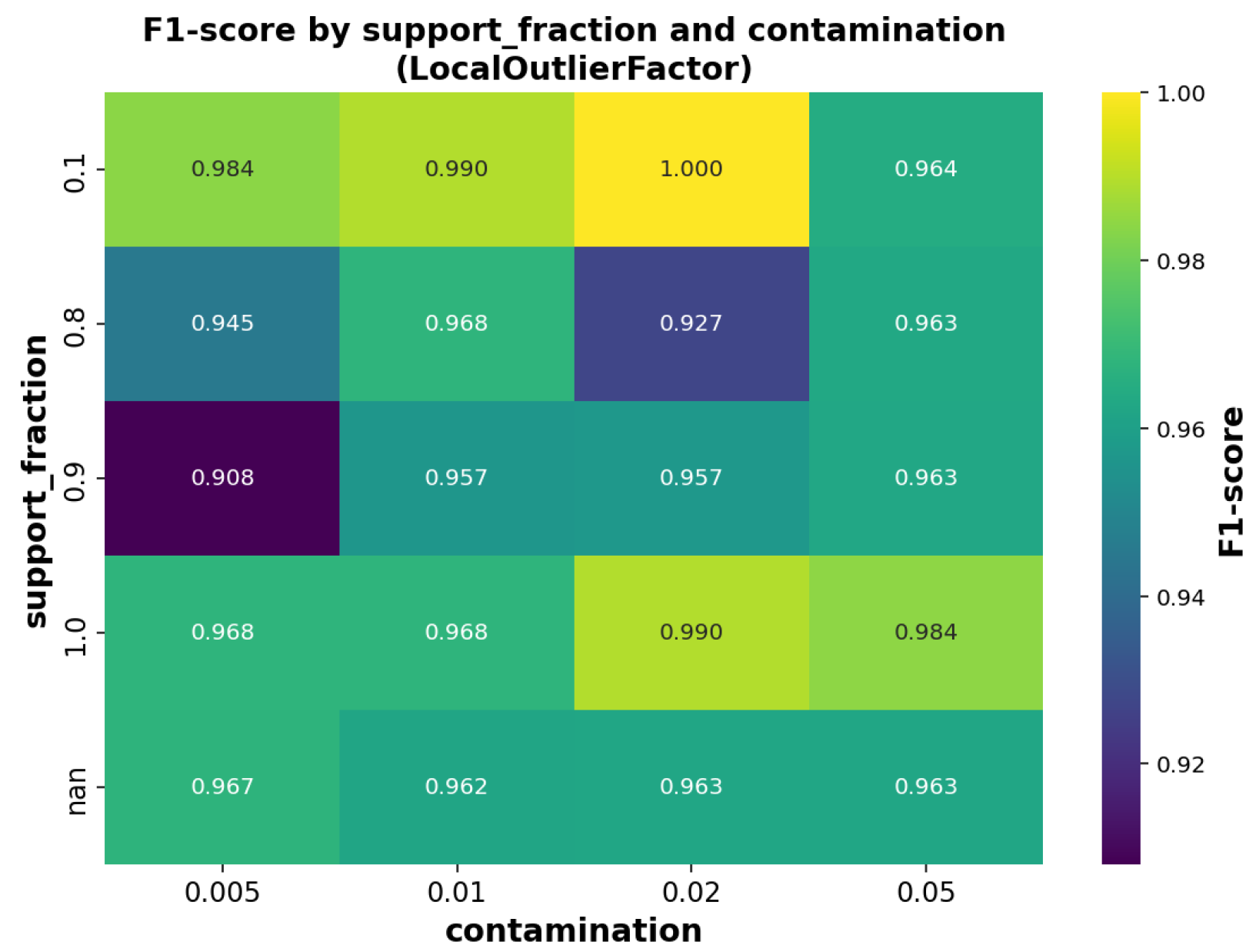
Figure 7. For the OCLOF model, the sensitivity of the F1-score was evaluated against different values of contamination and
n_neighbors, with results shown in
Figure 8. These visualizations facilitated selecting suitable configurations for each classifier, tailoring them to the specific characteristics of the data used in this study.
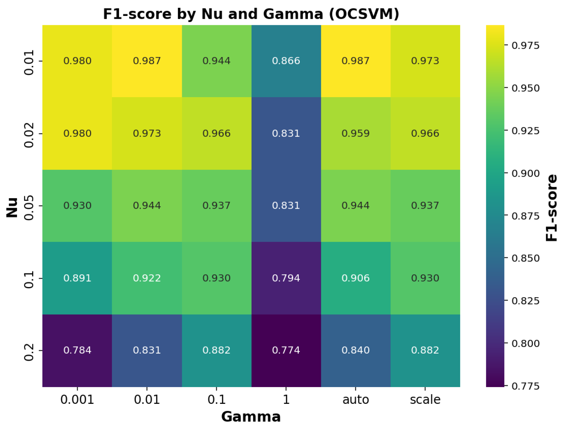
In the case of the OCSVM model, different combinations of the parameters
and
were tested, and their impact on the F1-score is shown in
Figure 9. This figure illustrates how the algorithm’s performance varies with these parameter values, enabling identification of the optimal configuration for our dataset.
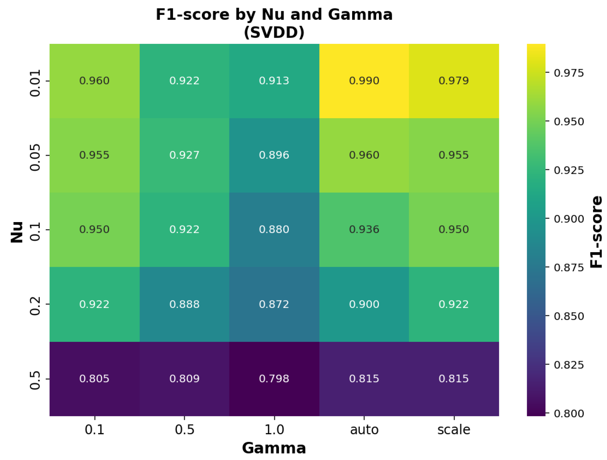
A similar evaluation was carried out for the SVDD model, where the influence of the
and
parameters on the F1-score is illustrated in
Figure 10.
Finally, the OCAutoencoder model was analyzed by modifying the number of neurons and the dropout rate. The resulting F1-score distribution is displayed in
Figure 11, aiding in the selection of the most effective architecture.
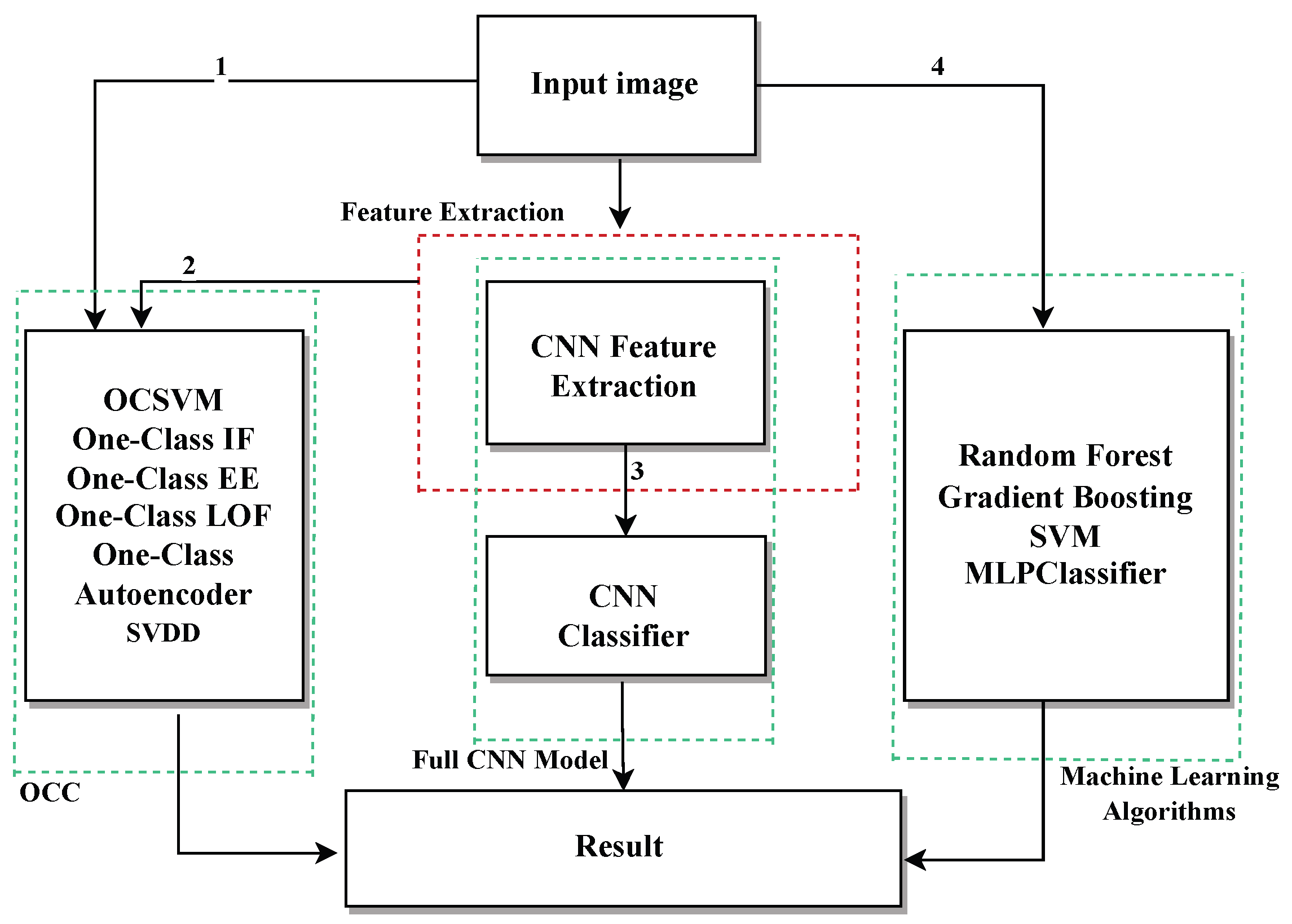
Before presenting the specific results,
Figure 12 summarizes the overall workflow of the proposed approach. Starting from preprocessed images, different analysis paths are explored:
Path 1: Images are directly input into unsupervised models such as OCSVM, OCAutoencoder, OCLOF, OCIF, and OCEE.
Path 2: Images are processed by a CNN trained as a feature extractor. The resulting representations are used as input for the unsupervised models.
Path 3: Images are directly classified by a CNN trained in a supervised manner.
Path 4: Images are classified using traditional machine learning algorithms such as SVM, Random Forest, Gradient Boosting, and MLPClassifier, which are trained on extracted features or augmented data.
5.1. Supervised and Unsupervised Models Using Raw Images as Input
In this first approach, anomaly detection algorithms were applied directly on the raw image data without any prior feature extraction. This methodology allows us to evaluate how effective traditional models are when faced with complex visual data without the support of deep representations.
As shown in
Table 3,
Table 4 and
Table 5, the overall performance of these models is limited, with precision, recall, and accuracy values significantly lower than those observed in other approaches. This highlights the difficulty that unsupervised classifiers have in learning relevant patterns directly from high-dimensional visual data.
5.2. Analysis of Traditional Machine Learning Algorithms
Table 6 presents the performance metrics of traditional machine learning algorithms applied to the test set containing 5% affected data with data augmentation.
It can be observed that all models achieve very high performance in detecting the majority class (class 1, unaffected), with recall values close to 100%. However, the performance in detecting the minority class (class 0, affected) is largely insufficient.
For instance, Random Forest and Gradient Boosting fail to correctly identify any affected instances (0% recall for class 0), indicating that they classify nearly all samples as unaffected. This results in high specificity but zero sensitivity toward affected cases.
The multi-layer perceptron (MLPClassifier) shows minimal affected detection capability, with precision and recall values around only 1%.
On the other hand, SVM stands out by demonstrating a better balance, achieving higher sensitivity and precision for affected detection (class 0), both around 71%, while maintaining excellent performance for the unaffected class.
These results highlight that, under strong class imbalance conditions, traditional machine learning algorithms tend to bias predictions towards the majority class, compromising effective affected case detection. This underscores the need for specific techniques or models to address class imbalance and improve minority class detection.
5.3. Supervised Classification with the CNN
Table 7 shows the results obtained when training the CNN model with different proportions of affected images. When only 5% of the training data belong to the affected class, the model exhibits very limited performance: although it achieves a recall of 100% for the affected class, its precision is extremely low (6.3%), indicating a high number of false positives. This behavior is expected since, with such a small number of representative samples, the neural network is unable to adequately learn the patterns that characterize this class.
When the proportion of affected images is increased to 50%, the performance improves significantly. The model reaches a precision of 97.62% and an F1-score of 93.36% for the affected class, demonstrating that with greater representation of the minority class, the CNN can learn more effective decision boundaries.
Finally, when 80% of the training data belong to the affected class, the model achieves perfect precision and recall (100%) for both classes. Although this result shows the model’s maximum potential, it does not represent a realistic scenario, as in most anomaly detection cases, anomalous data are scarce. However, this experiment serves as validation of the CNN’s strong learning capability when provided with sufficient balanced data.
These results highlight a common limitation of supervised methods when faced with imbalanced datasets and justify exploring alternative approaches, such as semi-supervised or unsupervised methods, to address anomaly detection problems in real-world contexts.
5.4. Unsupervised Models with Features Extracted via the CNN
This section is subdivided into four parts according to the hyperparameter optimization method used to improve the performance of unsupervised classifiers (OCC). In all cases, the inputs are feature vectors extracted by a previously trained CNN.
To enhance the performance of these classifiers, four tests were conducted, each using a different method for hyperparameter selection. This allows us to compare the impact of each technique on anomaly detection capability.
5.4.1. Test 1: Optimization Using the RandomizedSearchCV Algorithm
In this test, a heuristic approach is employed to select the hyperparameters. Below are the results obtained with the classifiers using this configuration (see
Table 8):
The algorithms OCSVM and SVDD stand out as the best models overall. Both present very high performance metrics in all categories, indicating a robust ability to distinguish between normal and affected instances. Additionally, they minimize both false positives and false negatives, maintaining high reliability in their predictions.
OCIF also offers solid performance, with high precision, recall, and F1-score values. Although its performance is slightly inferior to that of OCSVM and SVDD, it remains a reliable option in contexts requiring good detection capability with low error.
OCAutoencoder shows moderately high performance, especially in detecting normal instances. However, its precision slightly decreases for the affected class, implying a higher likelihood of false alarms or classification errors in that class.
EllipticEnvelope presents fair performance, with acceptable metrics, but they are notably lower than those of the best models. Its precision and ability to correctly discriminate classes are limited, especially in avoiding false positives.
OCLOF is the worst-performing model among those evaluated. Its precision and accuracy are considerably lower, with a high number of false positives. This suggests a limited capacity for reliable classification, making it a less recommended choice for sensitive scenarios.
5.4.2. Test 2: Optimization Using a Genetic Algorithm
The analysis of the average results of algorithms optimized by the genetic algorithm shows an overall excellent performance in anomaly detection for both classes. In general, the OCSVM, EllipticEnvelope, and OCLOF algorithms present the best performance, with precision, recall, F1-score, and accuracy metrics practically perfect, all close to or equal to 100%. This reflects an outstanding ability to correctly identify both normal and affected instances, with a practically negligible number of false positives and false negatives.
OCIF also delivers very good results, with slightly lower metrics but still above 98%, indicating solid performance, though not as perfect as the previous ones.
On the other hand, OCAutoencoder shows a more moderate performance. Although its precision for class 0 is high, the detection of class 1 is notably lower, with significantly reduced recall and F1-score. This suggests that this algorithm misses a relevant number of positive cases, which may affect its usefulness in applications where precise detection is critical.
Finally, SVDD ranks as the algorithm with the worst relative performance. It shows low recall for class 1, indicating a limited ability to detect positive cases. Despite maintaining high precision for class 0, its lower overall accuracy and AUC reflect a less favorable balance between false positives and false negatives. These results are presented in
Table 9.
5.4.3. Test 3: Optimization via the Bayesian Optimization Algorithm
Table 10 summarizes the performance results of algorithms optimized via Bayesian optimization. With optimization via Bayesian optimization, notable differences are observed among the evaluated algorithms. Overall, OCSVM, SVDD, and OCIF achieved the best overall results, demonstrating a high capacity to correctly identify both normal and affected instances. These models present a combination of high precision, recall, and F1-score metrics along with a superior AUC, indicating a very robust and balanced performance.
The autoencoder also showed notable performance, especially in the normal class, with metrics close to the best algorithms. However, it has a slight disadvantage compared to the others in detecting affected cases, which can be relevant in contexts sensitive to false negatives.
OCEE had an intermediate performance. While its ability to detect normal instances is notable, its performance was more limited when identifying affected cases. This translates into a lower overall balance in its metrics, reflecting unequal sensitivity between classes.
Finally, OCLOF was the algorithm with the worst overall performance. Its precision and discrimination ability were clearly inferior, affecting its practical utility in scenarios requiring reliable detection. Its performance was especially weak in the affected class, with a high proportion of errors.
5.4.4. Test 4: Optimization via the GridSearchCV Algorithm
Table 11 presents the evaluation metrics of algorithms tuned using the GridSearchCV method. In this analysis of anomaly detection algorithms, clear differences were observed in the performance of the models when evaluating standard metrics. OCSVM and OCIF were the algorithms with the best overall performance. Both achieved very high precision and recall values, exceeding 97% in most cases. In particular, OCSVM achieved an AUC above 99%, and OCIF also remained in that range, indicating an excellent discriminatory ability between normal and anomalous classes. Additionally, they presented the highest accuracy rates with very consistent results across both classes. On the other hand, the autoencoder and LOF showed intermediate performance. Although the autoencoder reached good precision in the anomalous class (94%), its recall was reduced (81%), meaning that it did not detect all positives, lowering its F1-score. LOF maintained a balanced performance, with metrics around 90%, neither standing out negatively nor as the best. EllipticEnvelope showed one of the worst performances. Despite a high recall score in class 0, its precision dropped below 60% due to a large number of false positives. Its AUC was the lowest of the group, evidencing its poor ability to correctly separate both classes. SVDD also showed clear limitations, especially in detecting the normal class, where its recall dropped significantly. Although it achieved 100% recall in anomalies, its precision was much lower, reflecting a tendency to overfit when detecting positives.
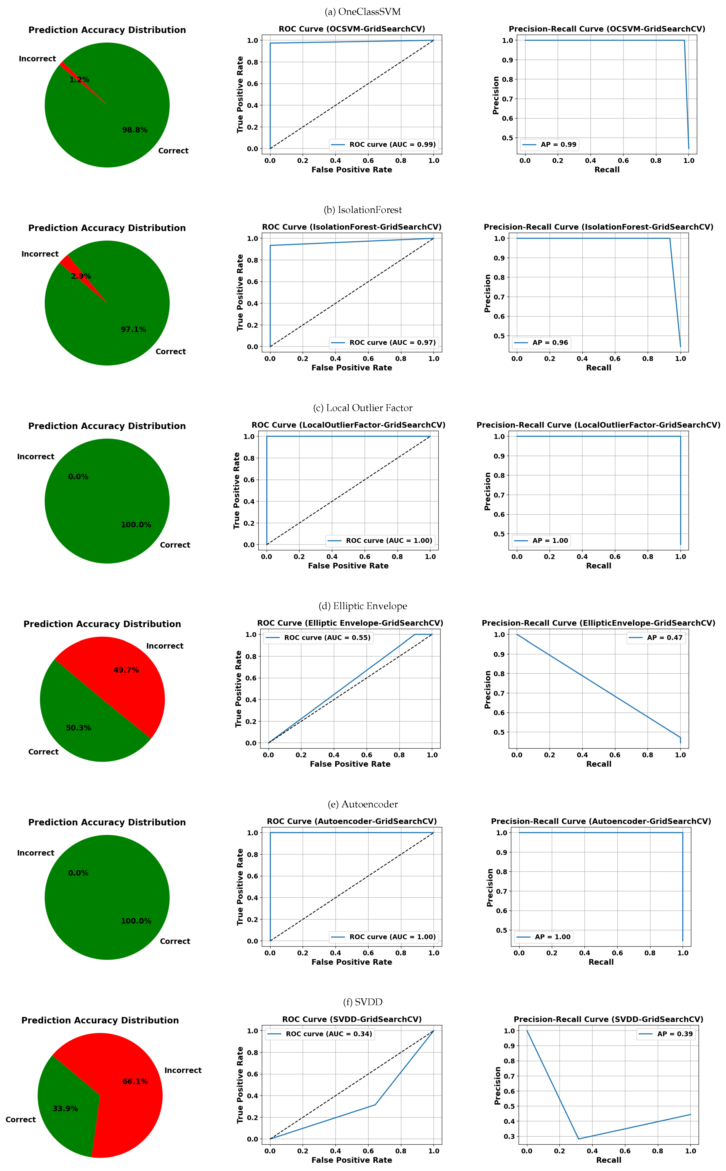
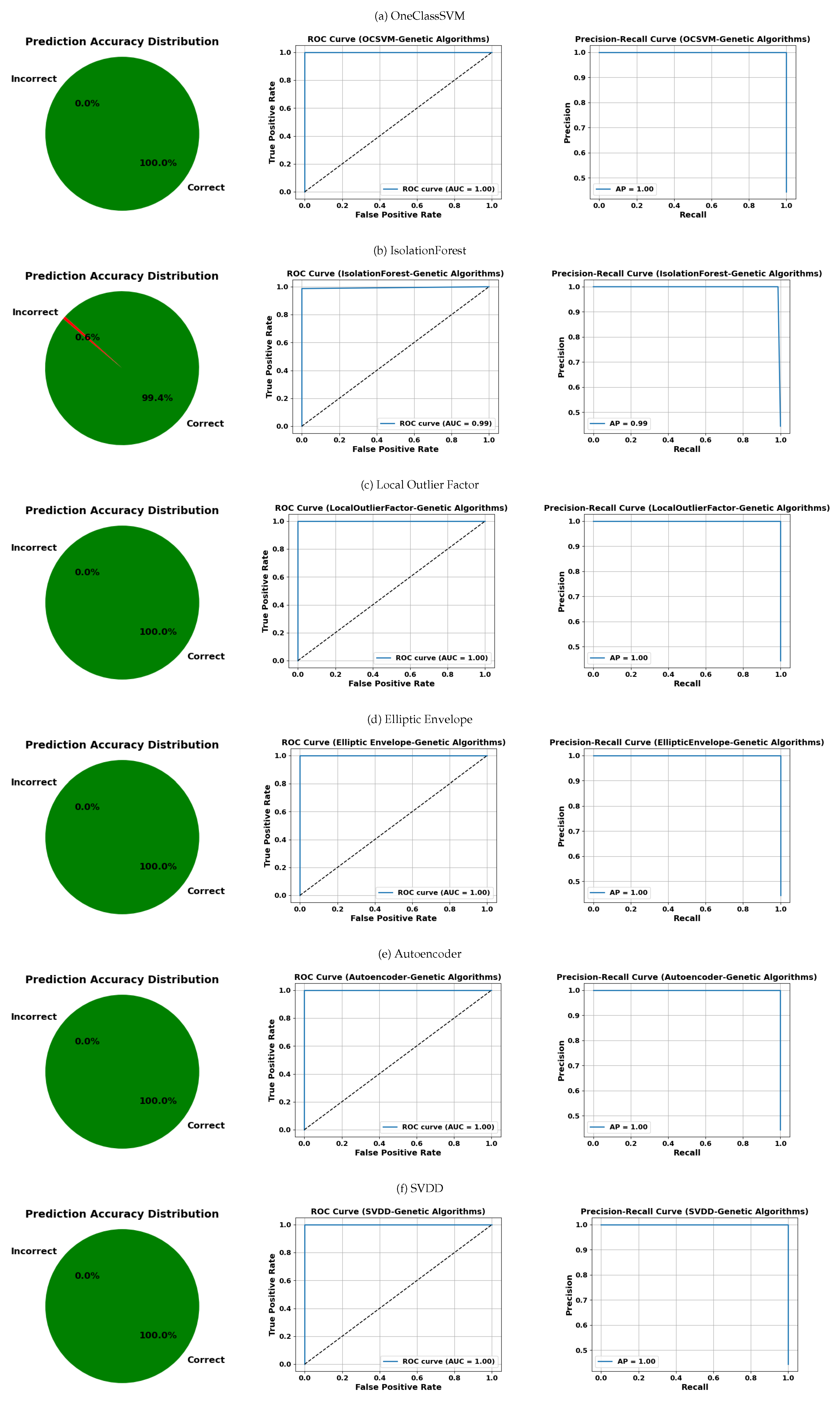
5.5. Visual Evaluation and Additional Metrics
The visual assessment shown in
Figure 13,
Figure 14,
Figure 15 and
Figure 16 complements the quantitative results by comparing various anomaly detection algorithms based on OCC. These visualizations include three types of plots per model: the distribution of correct and incorrect predictions, the ROC curve, and the PR curve, arranged from right to left. In each table, the rows represent the evaluated models—OCSVM, IF, LOF, EE, the autoencoder, and SVDD—while each table corresponds to a distinct hyperparameter optimization strategy: GridSearchCV, RandomizedSearchCV, Bayesian optimization, and genetic algorithms.
In
Figure 13, which presents results using GridSearchCV, LOF and Autoencoder stand out with 0% prediction errors and perfect AUC and AP scores of 1.00. OCSVM and IF also achieve high metrics (AUC and AP ≥ 0.96), although IF shows a slightly higher prediction error rate (2.9%). In contrast, EE and SVDD exhibit significantly lower performance, with error rates of 49.7% and 66.1%, respectively, and considerably lower AUC and AP values.
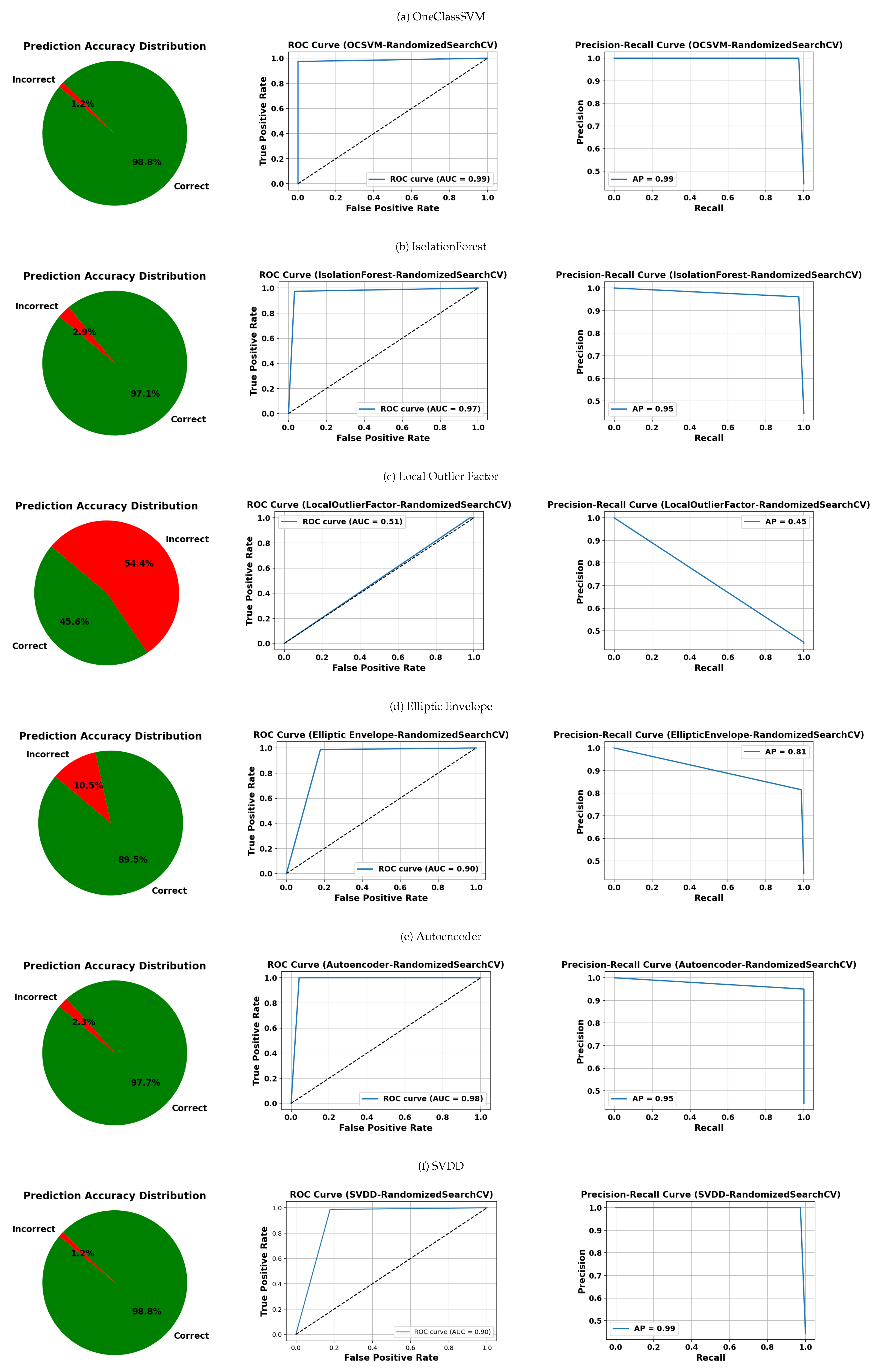
Figure 14, corresponding to RandomizedSearchCV, maintains OCSVM as one of the most stable models, with minimal errors and AUC/AP scores of 0.99. The autoencoder and SVDD also perform well (errors ≤ 2.3% and AUC/AP ≥ 0.90). However, LOF shows significant degradation, with over 54% prediction errors and metrics below 0.55, indicating high sensitivity to this random search method.
In
Figure 15, which employs Bayesian optimization, IF and SVDD stand out with 0.6% and 0% prediction errors, respectively, and near-perfect AUC/AP scores (≥0.99). OCSVM also performs well, but the autoencoder surprisingly yields AUC = 0.50 and AP = 0.44, possibly indicating overfitting or suboptimal configuration. Once again, EE and LOF display inconsistent results, with error rates exceeding 38%.
Finally,
Figure 16, associated with the genetic algorithms’ optimization strategy, shows remarkably uniform results: all models, except OCSVM (with 0.6% errors), achieve perfect prediction (0% errors) and maximum AUC and AP values (1.00). This indicates that this strategy was particularly effective for hyperparameter tuning across all OCC models evaluated.
These results confirm the strong capability of OCC models to detect anomalies with high precision, provided that they are supported by an appropriate hyperparameter optimization strategy. The observed differences between models and optimization methods underscore the need for careful selection of both the algorithm and the tuning approach. In this regard, genetic algorithms emerged as the most effective strategy, achieving optimal and consistent performance across all evaluated models.
5.6. Comparison of Anomaly Detection Performance
This section analyzes and compares the performance of various anomaly detection methods, including our proposed models (OCSVM and SVDD), using metrics such as precision, recall, specificity, the F1-score, and AUC. The results are summarized in
Table 12, incorporating data from the literature.
Our One-Class classification models show outstanding performance. Specifically, the OCSVM model achieved a precision of 97.37% and a recall of 100%, yielding an F1-score of 98.67%. Likewise, SVDD reached 100% precision and 97.37% recall, with the same F1-score. For the negative class, SVDD maintained excellent results with a specificity of 100% and an F1-score of 98.96%. The AUC for both models was 0.99, confirming high discriminative power and generalization capacity.
In comparison, classical methods such as the Isolation Forest algorithm [
10] reported a precision of 83.4%, but no further metrics were available.
Among recent deep learning methods, the DPAE model proposed by Liu et al. [
32] achieves the best performance, with a precision of 96%, a recall of 92%, a specificity of 89%, an F1-score of 94%, and an AUC of 0.92. Traditional autoencoder-based approaches like AE(L2) and AE(SSIM) [
33] show moderate performance with F1-scores around 0.73–0.76 and AUCs below 0.70. VAE [
34], AnoGAN [
35], and GANomaly [
36] present variable results, with AUC values between 0.63 and 0.72.
Table 12 provides a unified view of these results, confirming that our OCSVM and SVDD models outperform both classical and recent deep learning-based methods and demonstrating their suitability for anomaly detection tasks, particularly under limited anomaly supervision.
6. Discussion
The results obtained in this study allow for an in-depth evaluation of the effectiveness of various anomaly detection algorithms applied to the visual inspection of candle jars, with a special focus on OCC due to the limited availability of defective data.
The comparative analysis between hyperparameter optimization methods—GridSearchCV, RandomizedSearchCV, Bayesian optimization, and genetic algorithms—revealed significant variability in model performance. Particularly, optimization through Bayesian optimization and genetic algorithms showed a positive impact on improving performance, reaching near-perfect AUC values in models such as OCSVM and the autoencoder. This confirms that the proper selection and tuning of hyperparameters is crucial for maximizing anomaly detection capability.
Regarding the evaluated algorithms, the OCSVM model proved to be a robust and reliable tool, achieving an excellent balance between precision and sensitivity, which is essential to identify defects with high fidelity without generating an excessive number of false positives. Isolation-based models, like OCIF, also showed good results when properly optimized, although they demonstrated greater sensitivity to tuning methods. On the other hand, more traditional or unsupervised techniques, such as OCLOF, exhibited more erratic performance and dependence on the optimization method used, limiting their applicability in scenarios with limited data.
The graphical visualization of ROC curves, the comparison between true and predicted labels, and the angular distribution of precision complement and corroborate these quantitative findings, allowing for an intuitive and detailed interpretation of each model’s behavior.
The use of OCC techniques in this context is particularly suitable, given that in real industrial environments, it is common to have abundant data of normal products but scarce examples of defective ones. This makes traditional supervised classification approaches unfeasible and highlights the importance of anomaly detection methods in maintainable high-quality standards.
In the experiments with the CNN model as a supervised classifier, we observed that its effectiveness was highly dependent on the balance of data. When both normal and affected classes were sufficiently represented (e.g., 50% or 80% affected data), the CNN demonstrated high precision and recall, proving its strong learning capacity. However, when only 5% of the training data were affected samples, the model failed to properly distinguish between the two classes, resulting in a high number of false positives and demonstrating poor generalization under conditions of data scarcity.
Interestingly, when combining CNN feature extraction with an OCC model using the same 5% affected data, the system was able to correctly classify the anomalies. This finding reinforces the importance of hybrid approaches in situations where data are highly imbalanced: while CNNs alone struggle with very few anomalous examples, their feature representations remain informative and can be effectively leveraged by OCC methods to perform anomaly detection.
The performance of the evaluated models—both the supervised CNN and unsupervised OCC—was measured using a standard set of metrics widely adopted in binary classification tasks. The metrics considered include overall accuracy, sensitivity, precision, the F1-score, and the area under the ROC curve.
The AUC value is obtained from the ROC curve, which depicts the trade-off between the TPR and the FPR. A higher AUC indicates better discriminative capability of the model between normal and affected classes.
In addition, PRCs were analyzed as another evaluation parameter, especially relevant for datasets with class imbalance. PRCs emphasize the trade-off between precision and recall, providing a more informative measure of performance when the positive class (affected cases) is rare.
Overall, the proposed models have outperformed traditional supervised machine learning algorithms, demonstrating superior capability in accurately detecting affected cases in comparison to classical approaches.
Finally, the integration of advanced hyperparameter optimization strategies, along with models capable of learning complex representations from normal data, provides an effective and adaptable solution for automated quality control, with potential for extension to other types of products or defects.
It is recommended to continue exploring the combination of models and optimization methods, as well as to expand and diversify the available normal data, to further strengthen the generalization and robustness of the system under real production conditions.
7. Conclusions
The experimental results obtained in this study validate the effectiveness of anomaly detection systems applied to industrial quality control, even in scenarios dominated by normal data with scarce defective samples. The proposed approach, combining CNNs with OCC algorithms, achieved outstanding performance, reaching perfect metrics in several cases. This demonstrates the system’s ability to generalize from predominantly non-defective data, effectively addressing the challenges faced by traditional supervised methods in highly imbalanced environments.
Key contributions include the hybrid CNN+OCC architecture, which offers flexibility and high precision, and the implementation of advanced hyperparameter optimization strategies—such as Bayesian optimization and genetic algorithms—that proved crucial for maximizing model performance. Targeted data augmentation for minority classes was also employed, enhancing the system’s generalization capabilities. Nonetheless, the direct CNN classifier exhibited limitations under severe class imbalance, and some OCC algorithms showed sensitivity to hyperparameter settings, highlighting important considerations for practical deployment.
Futur work: Given the high detection metric results obtained, future work will focus on working with more complex and varied data to improve the system’s reliability and robustness. This includes incorporating products with different formats and characteristics that simulate real production conditions.
Additionally, it will be essential to evaluate the system’s performance under real industrial conditions, considering variations in lighting, different camera angles, and uncontrolled environments. These tests will allow the solution to be adapted and validated for practical application in automated production lines.
The integration of advanced object detection techniques, such as R-CNN and YOLO, combined with unsupervised methods that require only a very limited amount of negative examples to detect anomalies, is also planned. This will facilitate not only the identification of defects but also their precise localization within the product.


