Author Contributions
Conceptualization, P.Z.; methodology, P.L.; software, P.L. and J.W.; validation, P.L.; formal analysis, P.L.; investigation, P.L.; resources, P.Z. and T.L.; data curation, P.L.; writing—original draft preparation, P.L.; writing—review and editing, P.L., P.Z., J.W., X.W., Y.M. and T.L.; visualization, P.L.; supervision, P.Z. and T.L.; project administration, P.Z. and T.L.; funding acquisition, P.Z. and T.L. All authors have read and agreed to the published version of the manuscript.
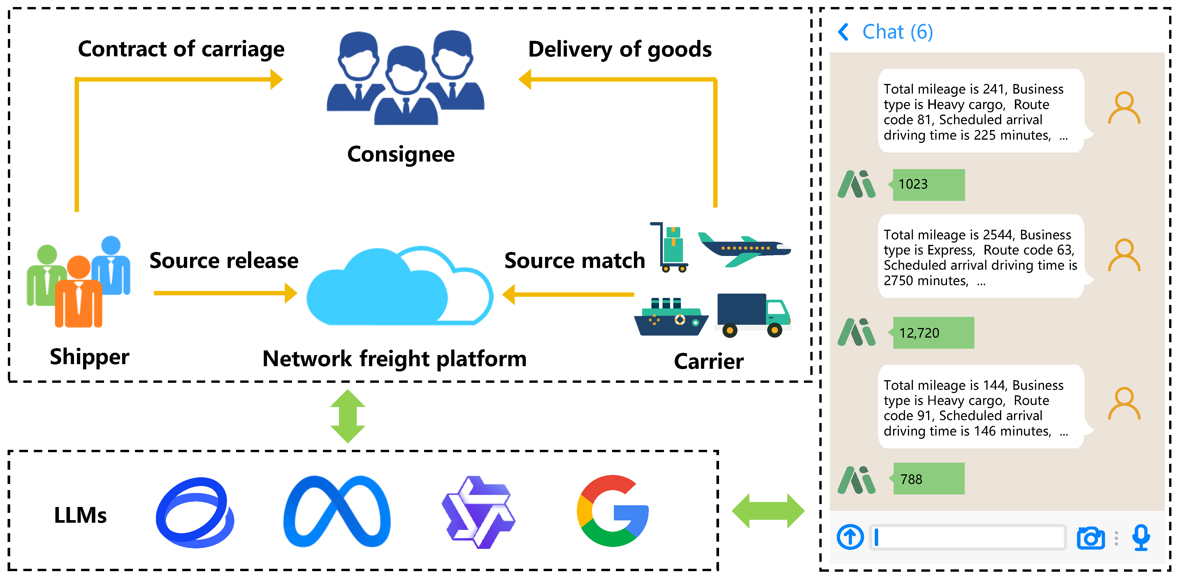
Figure 1.
Diagram of the logistics delivery process and key participants on the network freight platform.
Figure 1.
Diagram of the logistics delivery process and key participants on the network freight platform.
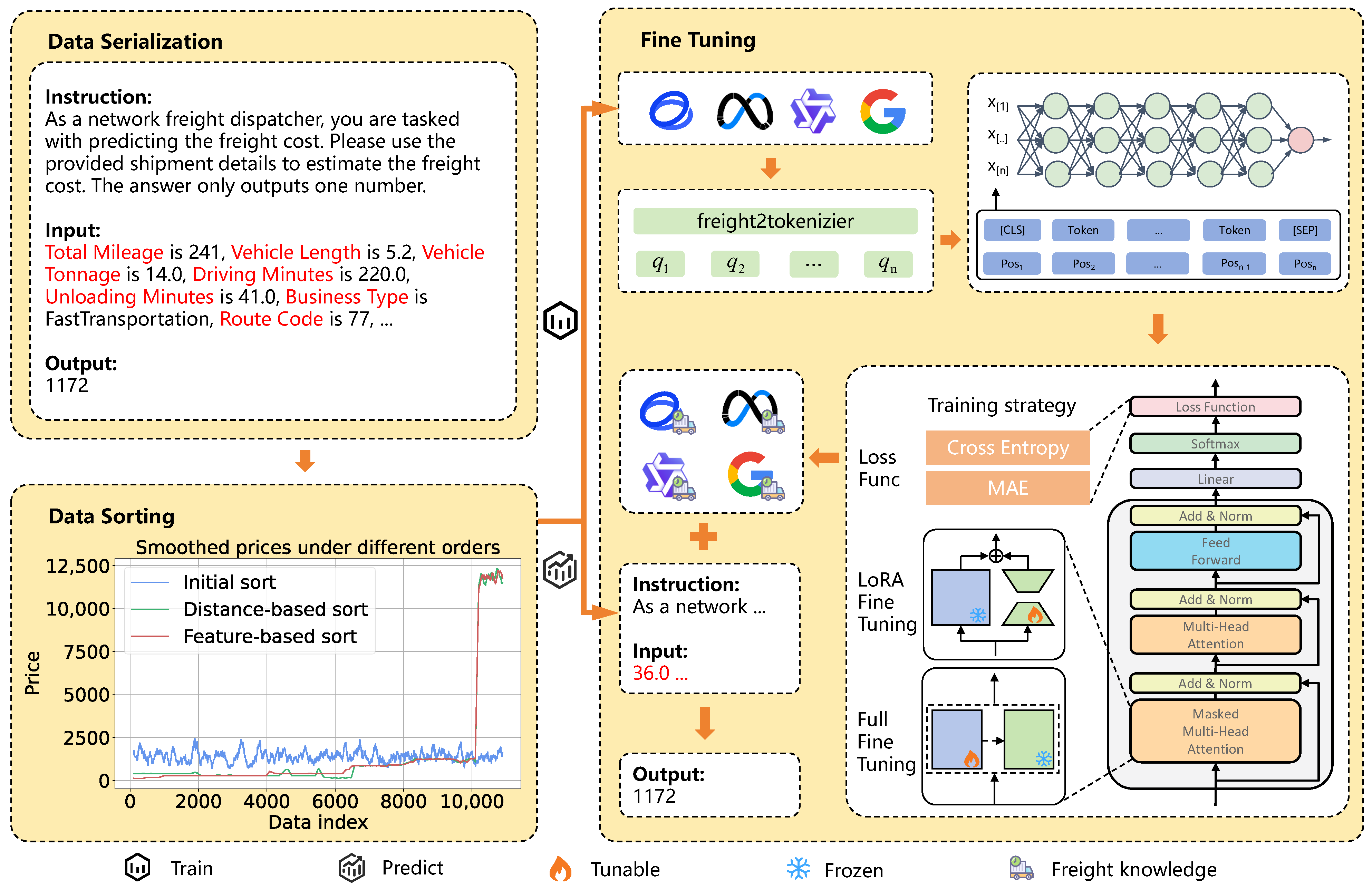
Figure 2.
Framework for network freight price prediction based on LLMs.
Figure 2.
Framework for network freight price prediction based on LLMs.
Figure 3.
Data serialization approaches in freight price prediction.
Figure 3.
Data serialization approaches in freight price prediction.
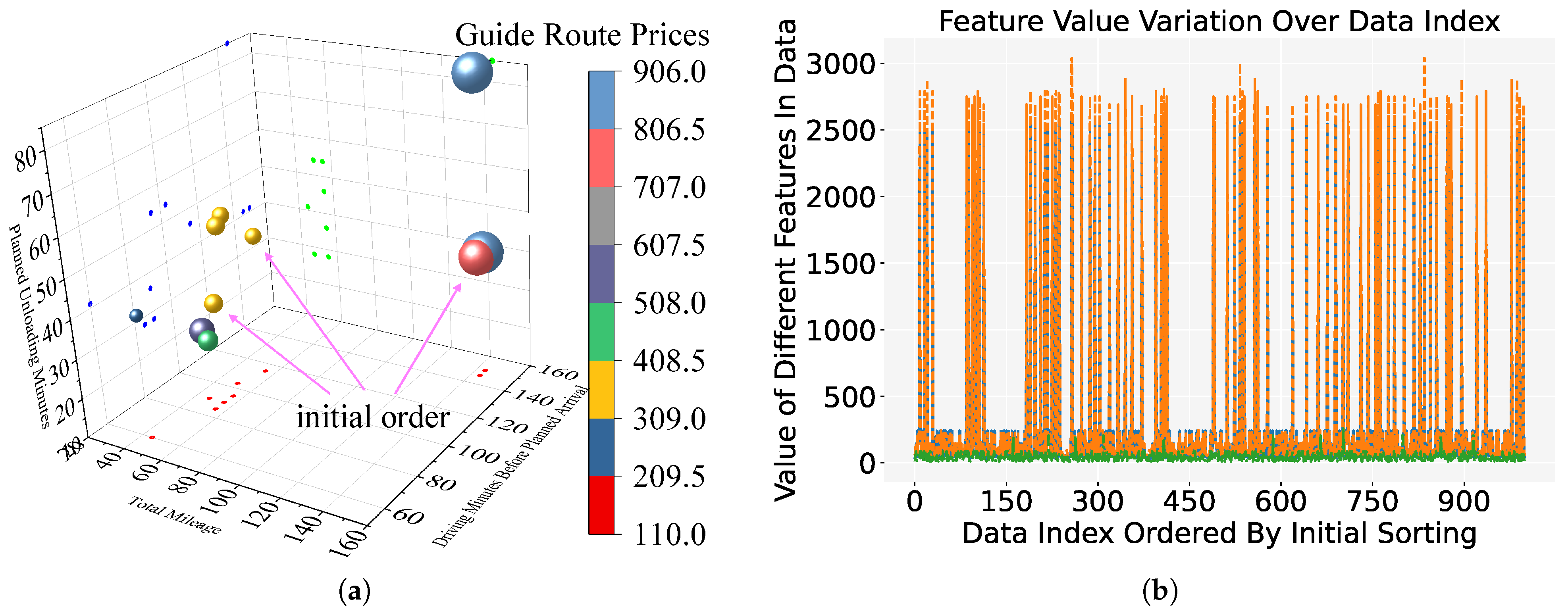
Figure 4.
Initial sort in the MathorCup dataset: (a) Demonstration in three-dimensional space; (b) Feature variation over the first 1000 data index. Blue represents Total Mileage, orange represents Driving Minutes Before Planned Arrival, and green represents Planned Unloading Minutes.
Figure 4.
Initial sort in the MathorCup dataset: (a) Demonstration in three-dimensional space; (b) Feature variation over the first 1000 data index. Blue represents Total Mileage, orange represents Driving Minutes Before Planned Arrival, and green represents Planned Unloading Minutes.
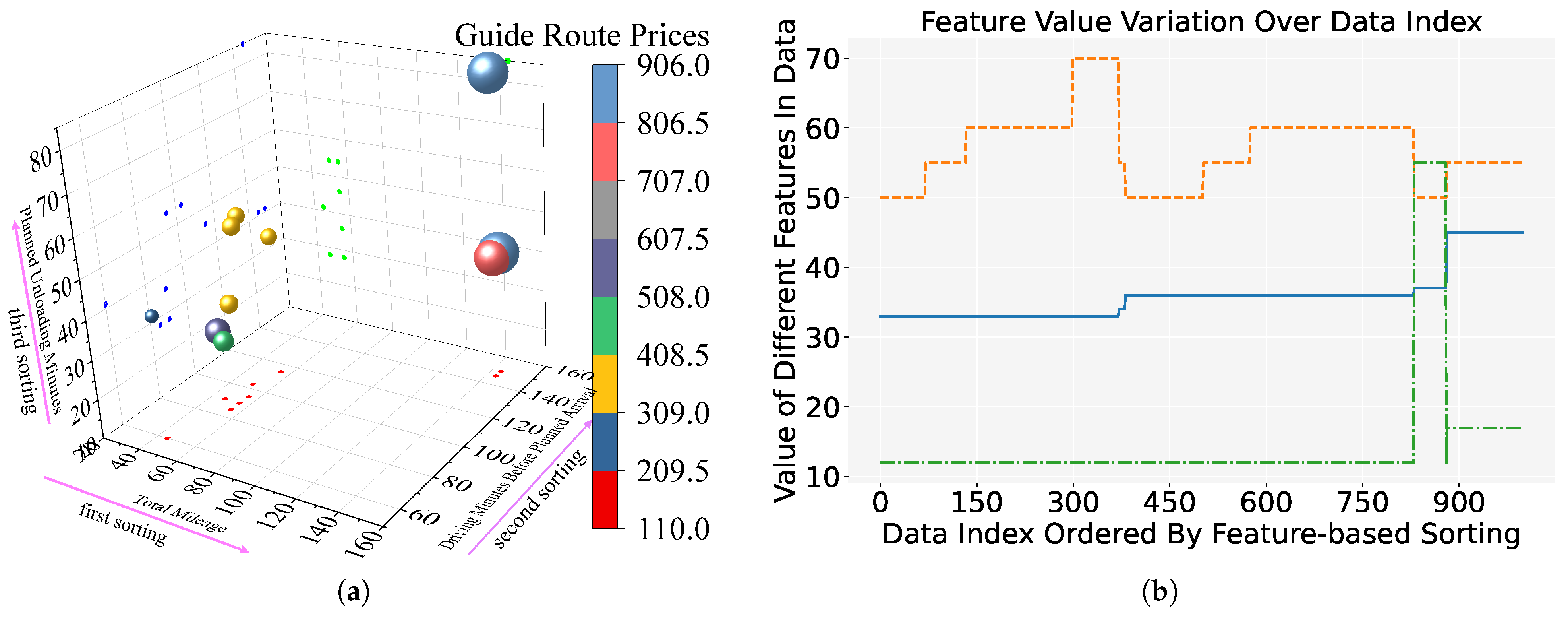
Figure 5.
Feature-based in the MathorCup dataset: (a) Demonstration in three-dimensional space; (b) Feature variation over the first 1000 data index. Blue represents Total Mileage, orange represents Driving Minutes Before Planned Arrival, and green represents Planned Unloading Minutes.
Figure 5.
Feature-based in the MathorCup dataset: (a) Demonstration in three-dimensional space; (b) Feature variation over the first 1000 data index. Blue represents Total Mileage, orange represents Driving Minutes Before Planned Arrival, and green represents Planned Unloading Minutes.
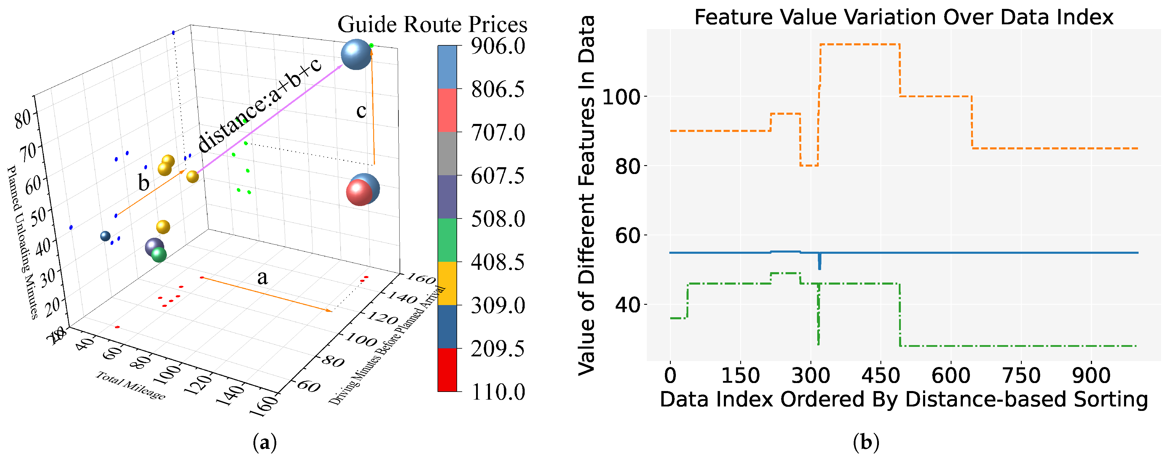
Figure 6.
Distance-based sort in the MathorCup dataset: (a) Demonstration in three-dimensional space; (b) Feature variation over the first 1000 data index. Blue represents Total Mileage, orange represents Driving Minutes Before Planned Arrival, and green represents Planned Unloading Minutes.
Figure 6.
Distance-based sort in the MathorCup dataset: (a) Demonstration in three-dimensional space; (b) Feature variation over the first 1000 data index. Blue represents Total Mileage, orange represents Driving Minutes Before Planned Arrival, and green represents Planned Unloading Minutes.
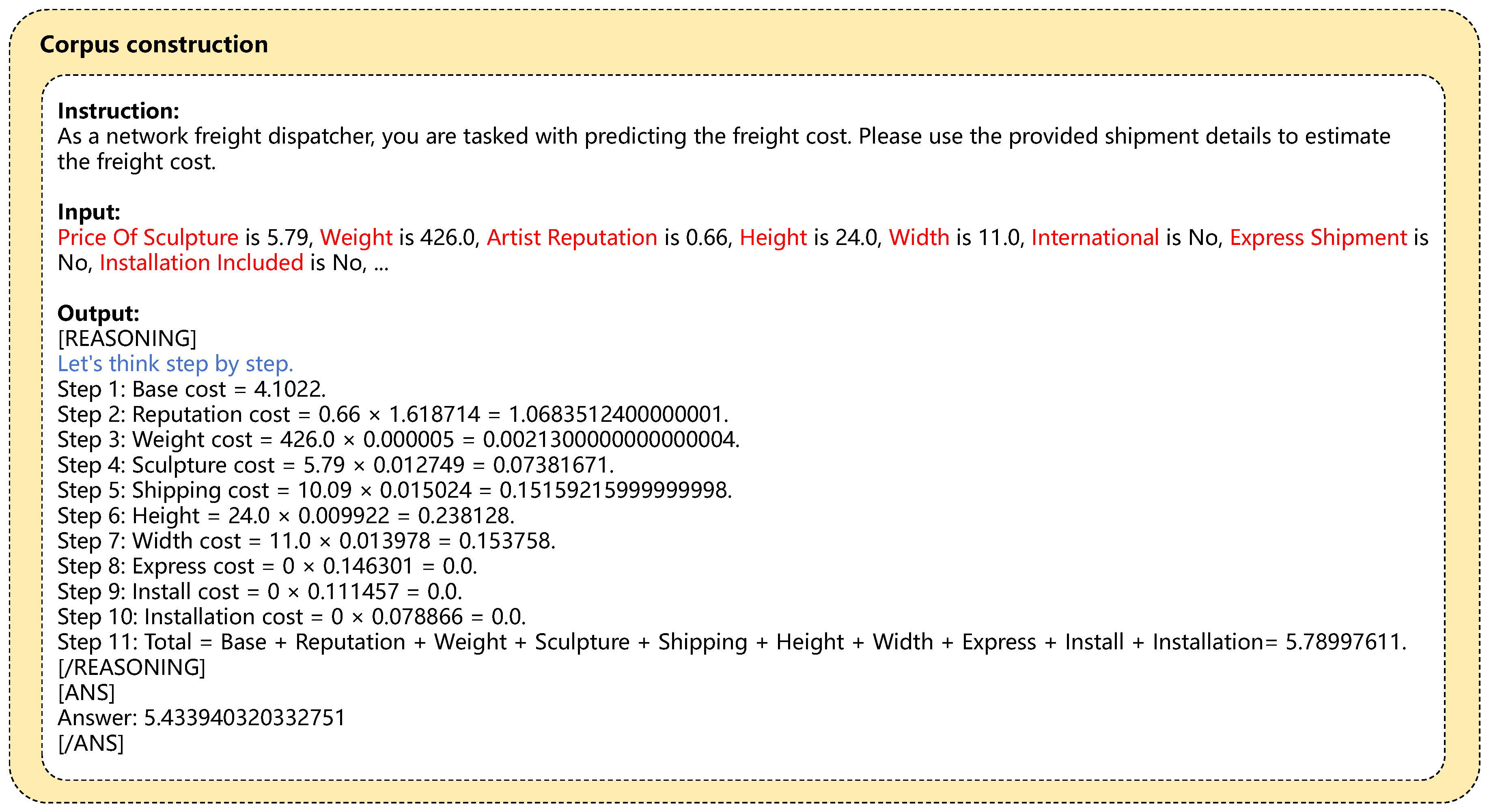
Figure 7.
Chain-of-thought prompting for MathorCup dataset. For better readability, line breaks have been added to the output section.
Figure 7.
Chain-of-thought prompting for MathorCup dataset. For better readability, line breaks have been added to the output section.
Figure 8.
Chain-of-thought prompting for HackerEarth dataset. For better readability, line breaks have been added to the output section.
Figure 8.
Chain-of-thought prompting for HackerEarth dataset. For better readability, line breaks have been added to the output section.
Figure 9.
Cosine annealing learning rate.
Figure 9.
Cosine annealing learning rate.
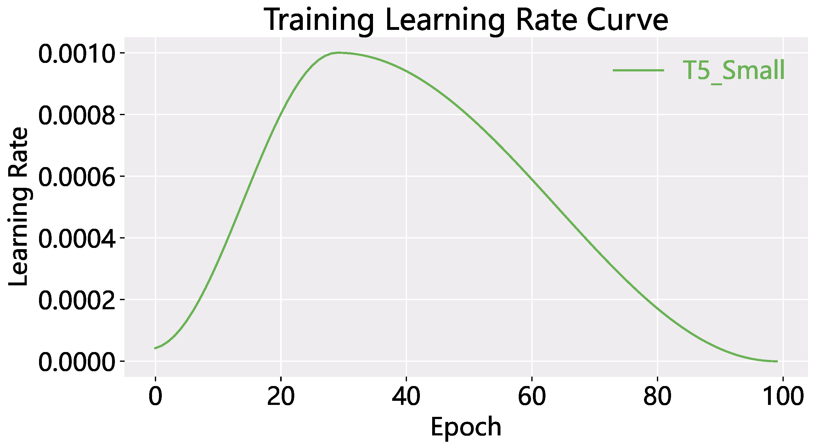
Figure 10.
OneCycle learning rate.
Figure 10.
OneCycle learning rate.
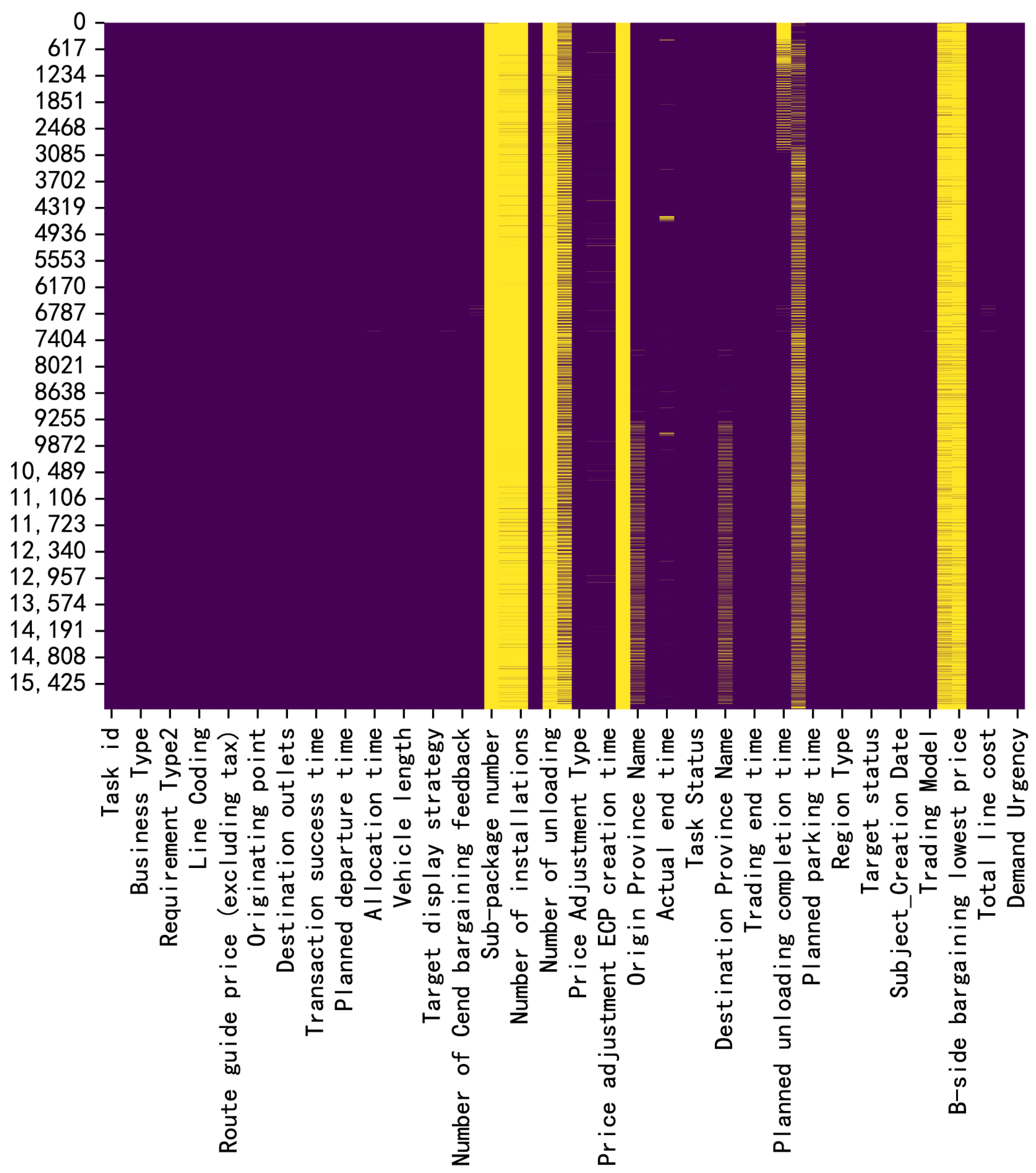
Figure 11.
Missing data in MathorCup dataset.
Figure 11.
Missing data in MathorCup dataset.
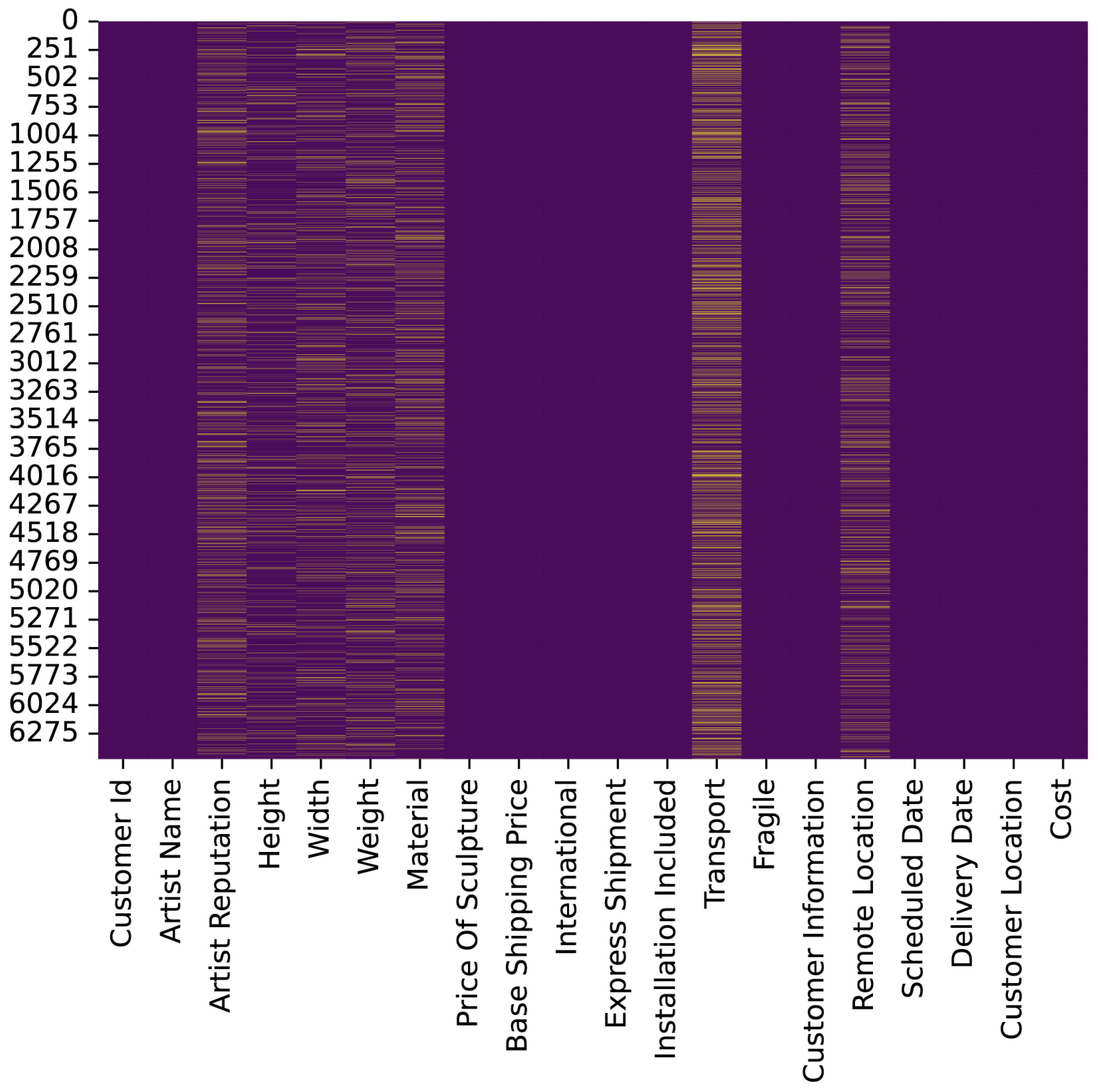
Figure 12.
Missing data in HackerEarth dataset.
Figure 12.
Missing data in HackerEarth dataset.
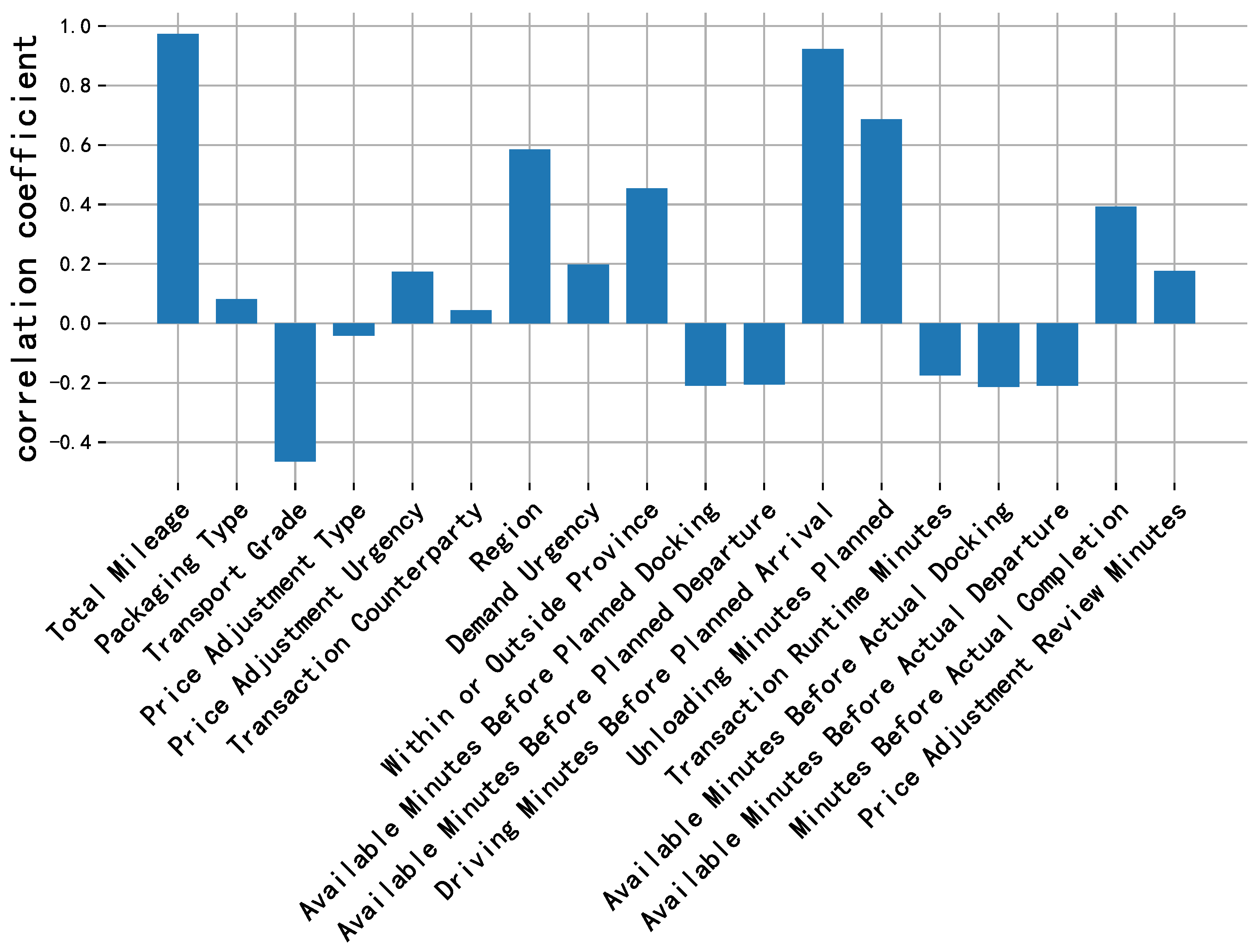
Figure 13.
Price correlation analysis of each feature in MathorCup dataset.
Figure 13.
Price correlation analysis of each feature in MathorCup dataset.
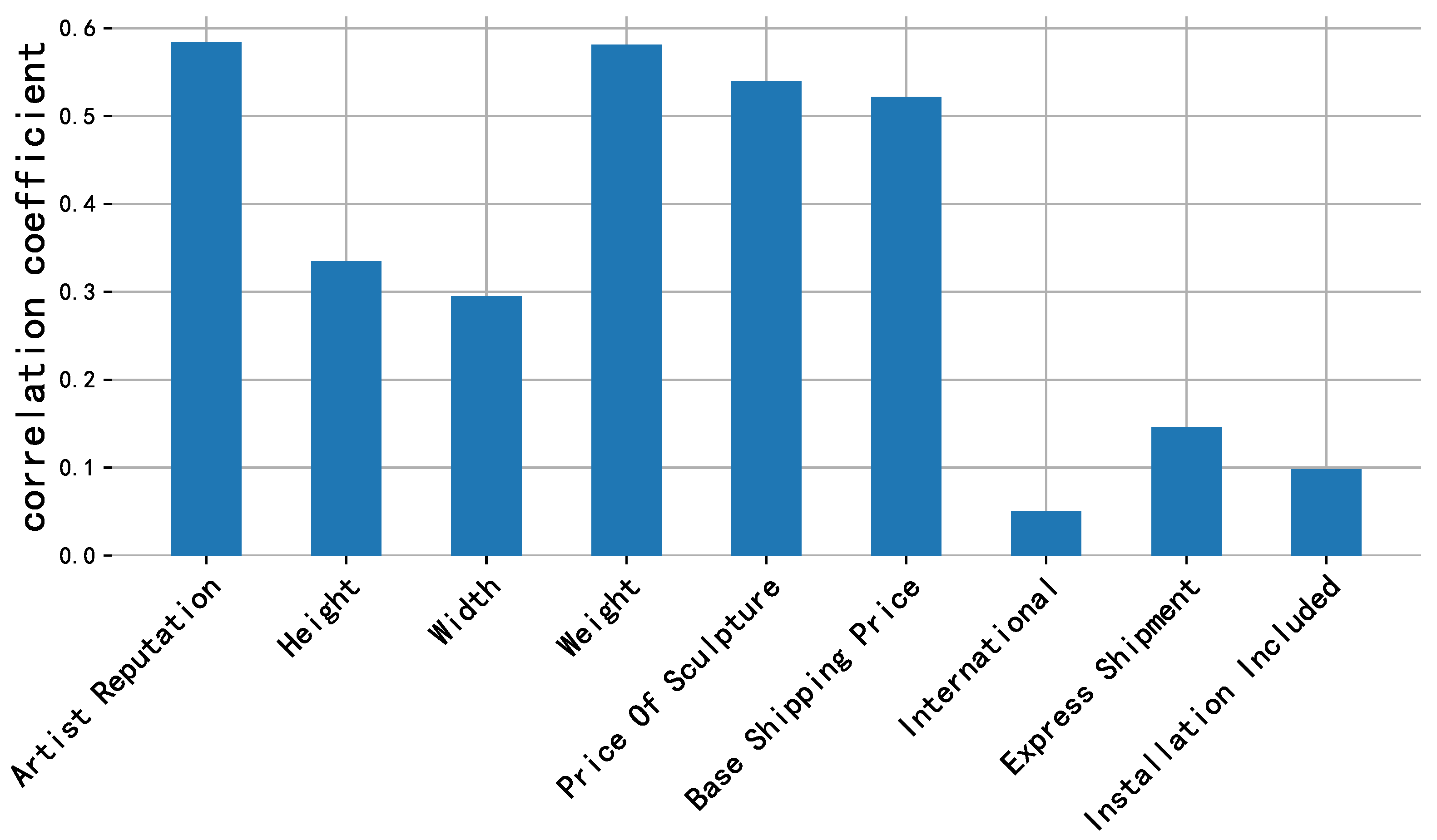
Figure 14.
Price correlation analysis of each feature in HackerEarth dataset.
Figure 14.
Price correlation analysis of each feature in HackerEarth dataset.
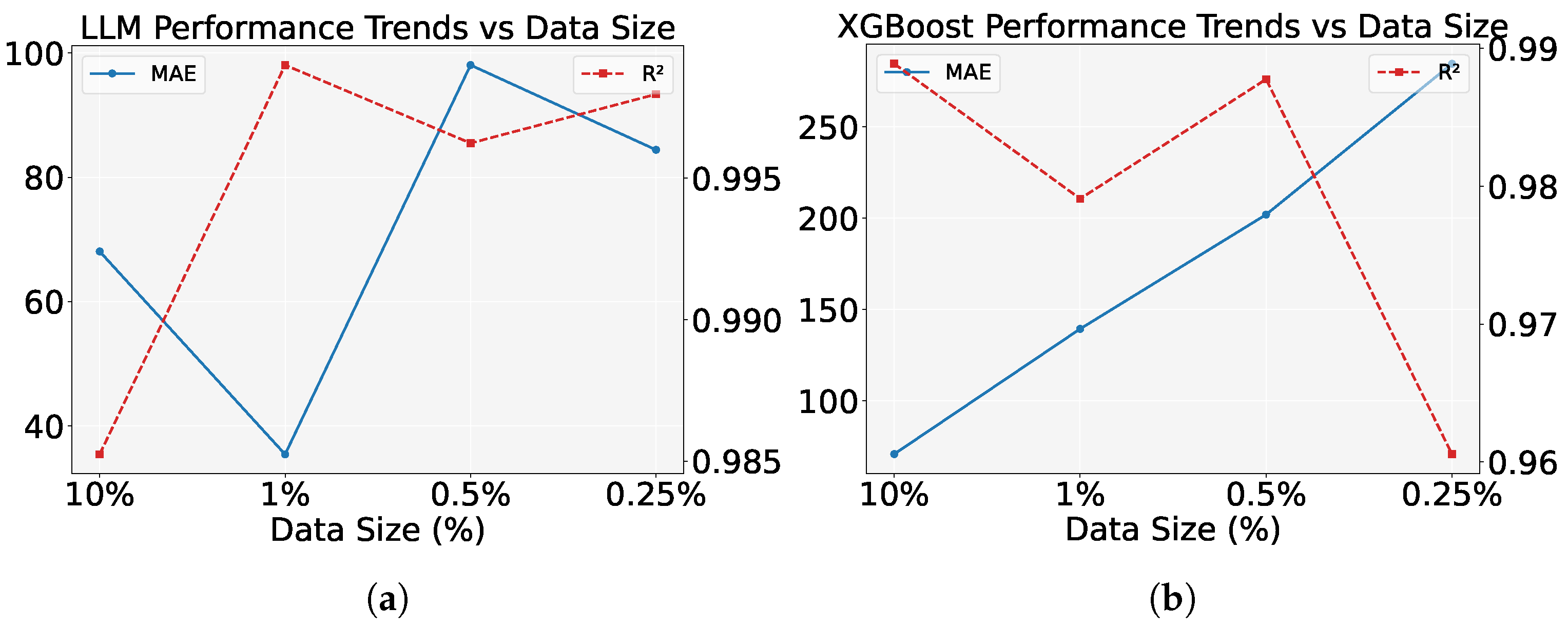
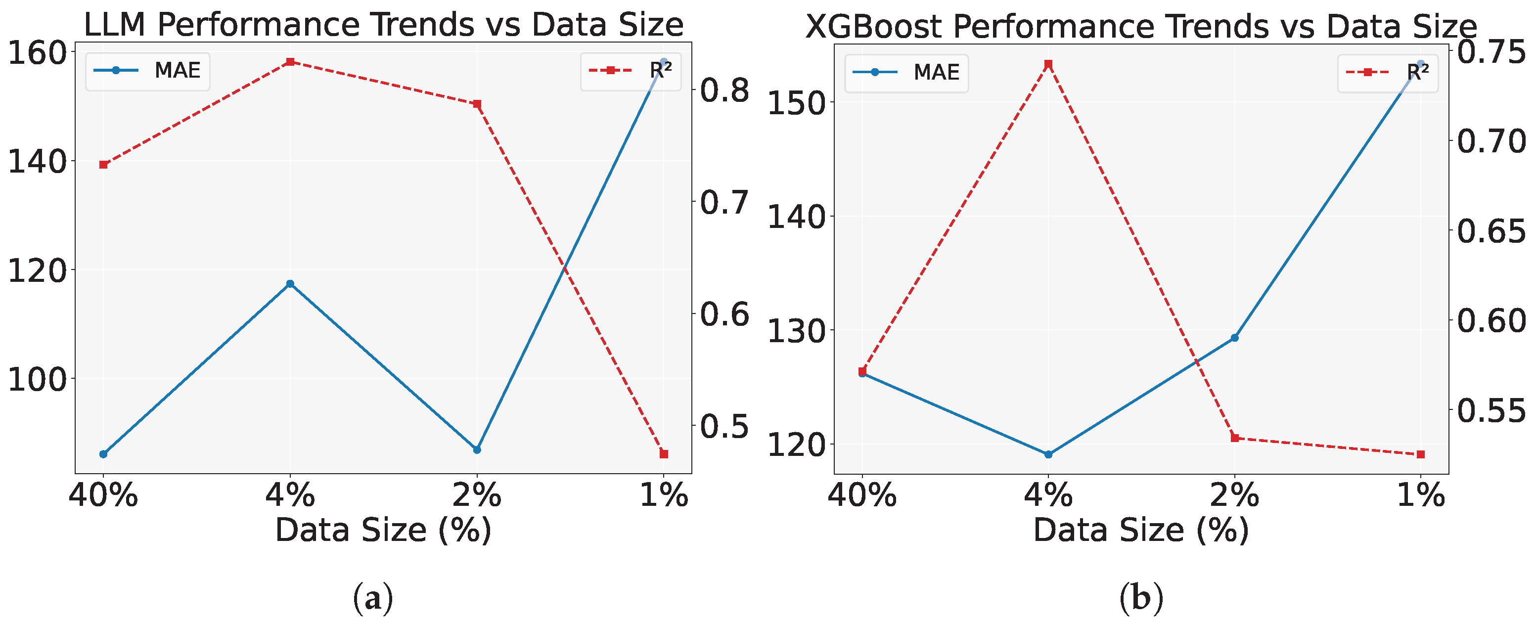
Figure 15.
Comparison of model performance trends with varying data size on the MathorCup dataset. (a) This subfigure shows the performance trends of the LLM model with respect to data size, using MAE and as metrics. The MAE increases as the data size decreases, and increases with smaller data sizes. (b) This subfigure shows the performance trends of the XGBoost model, comparing MAE and metrics. As the data size decreases, the MAE increases and decreases.
Figure 16.
Comparison of model performance trends with varying data size on the HackerEarth dataset. (a) This subfigure shows the performance trends of the LLM model with respect to data size, using MAE and as metrics. As the data size decreases, MAE increases and decreases. (b) This subfigure shows the performance trends of the XGBoost model, comparing the MAE and metrics. A similar trend is observed, with MAE increasing and decreasing as the data size decreases.
Table 1.
Definitions and clarifications of mathematical symbols.
Table 1.
Definitions and clarifications of mathematical symbols.
| Symbol | Dimension | Description |
|---|
| N | 1 | Total number of network freight orders. |
| P | 1 | Number of features in a network freight order. |
| C | 1 | Total number of prices in network freight orders. |
| 1 | The value is 1 when the i-th network freight order is predicted to have the c-th price; otherwise, it is 0. |
| 1 | The predicted probability of the i-th network freight order belonging to the c-th price. |
| 1 | Real price of the i-th network freight order. |
| 1 | Predicted price of the i-th network freight order by the model. |
| 1 | The i-th fundamental element of the token-sequence output. |
| X | | Network freight order feature data. |
| Y | N | Network freight order price data. |
Table 2.
Linear model performance varies with the number of features most relevant to price on MathorCup dataset.
Table 2.
Linear model performance varies with the number of features most relevant to price on MathorCup dataset.
| Top-K | MAE | MSE | MAPE | |
|---|
| 1 | 163.525 | 153,377 | 0.182099 | 0.983775 |
| 2 | 164.559 | 154,045 | 0.181416 | 0.983704 |
| 3 | 147.086 | 150,113 | 0.128677 | 0.984120 |
| 4 | 147.086 | 150,113 | 0.128677 | 0.984120 |
| 5 | 148.388 | 151,284 | 0.135270 | 0.983996 |
| 6 | 148.352 | 151,276 | 0.135085 | 0.983997 |
| 7 | 148.729 | 151,276 | 0.135738 | 0.983997 |
| 8 | 148.567 | 151,109 | 0.135800 | 0.984015 |
| 9 | 148.547 | 151,086 | 0.135817 | 0.984017 |
| all | 161.084 | 136,784 | 0.165328 | 0.985530 |
Table 3.
Linear model performance varies with the number of features most relevant to price on HackerEarth dataset.
Table 3.
Linear model performance varies with the number of features most relevant to price on HackerEarth dataset.
| Top-K | MAE | MSE | MAPE | |
|---|
| 1 | 0.440 | 0.319 | 0.074291 | 0.329808 |
| 2 | 0.331 | 0.216 | 0.055515 | 0.545345 |
| 3 | 0.314 | 0.180 | 0.052673 | 0.620787 |
| 4 | 0.247 | 0.117 | 0.041768 | 0.754109 |
| 5 | 0.221 | 0.097 | 0.037702 | 0.796323 |
| 6 | 0.219 | 0.096 | 0.037434 | 0.798213 |
| 7 | 0.219 | 0.094 | 0.037325 | 0.802006 |
| 8 | 0.216 | 0.092 | 0.036823 | 0.807407 |
| 9 | 0.212 | 0.089 | 0.036217 | 0.811891 |
| all | 0.192 | 0.079 | 0.032687 | 0.833838 |
Table 4.
Overview of dataset key features.
Table 4.
Overview of dataset key features.
| Dataset | Feature Name |
|---|
| MC | Total Mileage |
| Driving Minutes Before Planned Arrival |
| Unloading Minutes Planned |
| Transaction Runtime Minutes |
| Available Minutes Before Actual Docking |
| Available Minutes Before Actual Departure |
| Minutes Before Actual Completion |
| Price Adjustment Review Minutes |
| Available Minutes Before Planned Docking |
| Available Minutes Before Planned Departure |
| Packaging Type |
| Transport Grade |
| Price Adjustment Type |
| Price Adjustment Urgency |
| Transaction Counterparty |
| Region |
| Demand Urgency |
| Within or Outside Province |
| HE | Artist Reputation |
| Height |
| Width |
| Weight |
| Price Of Sculpture |
| Base Shipping Price |
| Area |
| Combined Price |
| International |
| Express Shipment |
| Installation Included |
| CO | Distance |
| Vehicle length |
| Vehicle type |
| Cargo weight |
| Cargo volume |
| Pick-up province |
| Unloading province |
| Transportation time |
| Holiday |
| Month |
| Price |
Table 5.
Overview of dataset sizes.
Table 5.
Overview of dataset sizes.
| Dataset | Description | Count |
|---|
| MC | Total Raw Entries | 16,016 |
| Raw Feature Dimensions | 63 |
| Total Preprocessed Entries | 13,615 |
| HE | Total Raw Entries | 6500 |
| Raw Feature Dimensions | 20 |
| Total Preprocessed Entries | 4001 |
| CO | Total Raw Entries | 36,000 |
| Raw Feature Dimensions | 14 |
| Total Preprocessed Entries | 33,195 |
Table 6.
Regional freight trends in MathorCup.
Table 6.
Regional freight trends in MathorCup.
| Region | Price Mean | Price Variance |
|---|
| 1 | 412.22 | 1919.98 |
| 2 | 152.88 | 984.12 |
| 3 | 491.03 | 80,545.38 |
| 4 | 11,871.47 | 1,985,854.00 |
| 5 | 1188.18 | 29,320.30 |
| 6 | 730.35 | 19,950.27 |
Table 7.
Transport freight trends in HackerEarth.
Table 7.
Transport freight trends in HackerEarth.
| Transport | Cost Mean | Cost Variance |
|---|
| Airways | 25,138.71 | |
| Roadways | 16,321.61 | |
| Waterways | 9187.90 | |
Table 8.
Library versions.
Table 8.
Library versions.
| Library Name | Current Version |
|---|
| transformers | ≥4.41.2 |
| datasets | ≥2.16.0 |
| accelerate | ≥0.30.1 |
| peft | ≥0.11.1 |
| trl | ≥0.8.6 |
| torchmetrics | 0.11.4 |
Table 9.
Performance of compared models in full data.
Table 9.
Performance of compared models in full data.
| Dataset | Model | MAE | MSE | MAPE | |
|---|
| MC | XGBoost | 12.036 | 6868 | 0.00453 | 0.999261 |
| LightGBM | 20.543 | 9525 | 0.01080 | 0.998975 |
| RF | 15.423 | 7409 | 0.00730 | 0.999203 |
| GBDT | 13.299 | 8670 | 0.00960 | 0.999067 |
| ExtraTrees | 12.782 | 9439 | 0.00438 | 0.998984 |
| DT | 24.448 | 11,873 | 0.01704 | 0.998723 |
| DNNs | 203.973 | 165,706 | 0.32918 | 0.982179 |
| PLS | 190.998 | 173,439 | 0.26772 | 0.981348 |
| Lasso | 155.075 | 133,631 | 0.15450 | 0.985629 |
| Ridge | 152.920 | 128,510 | 0.16307 | 0.986179 |
| ElasticNet | 145.528 | 146,988 | 0.14749 | 0.984192 |
| SVR | 1158.886 | 10,306,138 | 0.63346 | −0.108338 |
| KR | 153.193 | 128,584 | 0.16440 | 0.986171 |
| PCA | 137.174 | 146,294 | 0.13850 | 0.984267 |
| BR | 152.512 | 129,621 | 0.16105 | 0.986060 |
| HE | XGBoost | 128.068 | 113,079 | 0.23581 | 0.523815 |
| LightGBM | 145.901 | 140,377 | 0.26584 | 0.408859 |
| RF | 112.437 | 86,568 | 0.22128 | 0.635453 |
| GBDT | 98.204 | 77,988 | 0.17398 | 0.671584 |
| ExtraTrees | 137.114 | 117,320 | 0.26962 | 0.505957 |
| DT | 160.048 | 144,692 | 0.31006 | 0.390689 |
| DNNs | 250.959 | 264,763 | 0.50535 | −0.114936 |
| PLS | 168.751 | 141,021 | 0.33730 | 0.406149 |
| Lasso | 186.399 | 146,295 | 0.41760 | 0.383940 |
| Ridge | 93.682 | 58,309 | 0.17747 | 0.754455 |
| ElasticNet | 191.285 | 153,673 | 0.43078 | 0.352873 |
| SVR | 252.096 | 250,254 | 0.59910 | −0.053837 |
| KR | 93.351 | 57,823 | 0.17724 | 0.756500 |
| PCA | 93.634 | 58,350 | 0.17738 | 0.754284 |
| BR | 93.908 | 58,754 | 0.17693 | 0.752582 |
| CO | XGBoost | 441.196 | 1,119,809 | 0.18362 | 0.885241 |
| LightGBM | 584.293 | 1,153,242 | 0.26571 | 0.881815 |
| RF | 785.043 | 1,935,786 | 0.34883 | 0.801619 |
| GBDT | 440.845 | 1,251,295 | 0.17728 | 0.871766 |
| ExtraTrees | 740.413 | 1,577,908 | 0.36291 | 0.838295 |
| DT | 610.468 | 1,585,597 | 0.25134 | 0.837507 |
| DNNs | 539.212 | 1,083,497 | 0.21791 | 0.888962 |
| PLS | 970.893 | 2,472,120 | 0.48266 | 0.746655 |
| Lasso | 828.010 | 1,913,604 | 0.41144 | 0.803892 |
| Ridge | 827.111 | 1,910,470 | 0.41082 | 0.804214 |
| ElasticNet | 891.745 | 2,254,588 | 0.41789 | 0.768948 |
| SVR | 1723.153 | 10,142,073 | 0.61695 | −0.039364 |
| KR | 827.094 | 1,910,485 | 0.41080 | 0.804212 |
| PCA | 899.578 | 2,244,267 | 0.42656 | 0.770006 |
| BR | 828.079 | 1,912,611 | 0.41169 | 0.803994 |
Table 10.
Training parameters for cross entropy loss experiments.
Table 10.
Training parameters for cross entropy loss experiments.
| Dataset | Model | Loss Function | Epoch | Batch Size | Learning Rate |
|---|
| MC;CO | GLM | Cross Entropy | 5 | 1 | |
| Qwen | Cross Entropy | 5 | 1 | |
| Llama | Cross Entropy | 5 | 1 | |
| HE | GLM | Cross Entropy | 15 | 1 | |
| Qwen | Cross Entropy | 15 | 1 | |
| Llama | Cross Entropy | 15 | 1 | |
Table 11.
Performance of cross entropy loss in MathorCup full data.
Table 11.
Performance of cross entropy loss in MathorCup full data.
| Sort | Serialization | Model | MAE | MSE | MAPE | |
|---|
| IS | NFS | GLM | 9.250 | 8590 | 0.00426 | 0.999076 |
| NFS | Llama | 17.929 | 65,775 | 0.00666 | 0.992926 |
| NFS | Qwen | 25.766 | 36,025 | 0.01409 | 0.996125 |
| LTS | GLM | 11.502 | 14,221 | 0.00509 | 0.998470 |
| LTS | Llama | 11.990 | 12,671 | 0.00568 | 0.998637 |
| LTS | Qwen | 20.676 | 98,205 | 0.00603 | 0.989438 |
| VOS | GLM | 8.550 | 7616 | 0.00397 | 0.999180 |
| VOS | Llama | 12.215 | 12,786 | 0.00449 | 0.998624 |
| VOS | Qwen | 11.514 | 9791 | 0.00684 | 0.998946 |
| JS | GLM | 11.597 | 11,836 | 0.00434 | 0.998727 |
| JS | Llama | 13.388 | 13,641 | 0.00547 | 0.998532 |
| JS | Qwen | 14.247 | 11,295 | 0.00701 | 0.998785 |
| FS | NFS | GLM | 12.651 | 15303 | 0.00529 | 0.998354 |
| NFS | Llama | 14.429 | 23,675 | 0.00533 | 0.997453 |
| NFS | Qwen | 86.617 | 4,523,043 | 0.01537 | 0.513584 |
| LTS | GLM | 13.211 | 17,917 | 0.00533 | 0.998073 |
| LTS | Llama | 10.731 | 12,381 | 0.00503 | 0.998668 |
| LTS | Qwen | 18.692 | 54,918 | 0.00839 | 0.994093 |
| VOS | GLM | 13.038 | 46,614 | 0.00625 | 0.994986 |
| VOS | Llama | 17.133 | 61,115 | 0.00470 | 0.993427 |
| VOS | Qwen | 14.940 | 17,658 | 0.00499 | 0.998100 |
| JS | GLM | 11.355 | 12,491 | 0.00513 | 0.998656 |
| JS | Llama | 13.468 | 15,049 | 0.00590 | 0.998381 |
| JS | Qwen | 12.269 | 9261 | 0.00738 | 0.999004 |
| DS | NFS | GLM | 12.439 | 14,418 | 0.00452 | 0.998449 |
| NFS | Llama | 13.404 | 15,870 | 0.00755 | 0.998293 |
| NFS | Qwen | 34.860 | 113,884 | 0.01587 | 0.987752 |
| LTS | GLM | 11.040 | 11,449 | 0.00486 | 0.998768 |
| LTS | Llama | 10.108 | 10,873 | 0.00480 | 0.998830 |
| LTS | Qwen | 19.407 | 57,803 | 0.00822 | 0.993783 |
| VOS | GLM | 12.631 | 14,389 | 0.00592 | 0.998452 |
| VOS | Llama | 11.078 | 13,256 | 0.00378 | 0.998574 |
| VOS | Qwen | 13.283 | 9876 | 0.00625 | 0.998937 |
| JS | GLM | 12.341 | 14,000 | 0.00488 | 0.998494 |
| JS | Llama | 13.019 | 14,445 | 0.00558 | 0.998446 |
| JS | Qwen | 12.188 | 7475 | 0.00641 | 0.999196 |
Table 12.
Performance of cross entropy loss in HackerEarth full data.
Table 12.
Performance of cross entropy loss in HackerEarth full data.
| Sort | Serialization | Model | MAE | MSE | MAPE | |
|---|
| IS | NFS | GLM | 52.019 | 41,091 | 0.09127 | 0.826960 |
| NFS | Llama | 67.513 | 57,063 | 0.11394 | 0.759702 |
| NFS | Qwen | 59.806 | 34,408 | 0.10746 | 0.855104 |
| LTS | GLM | 53.893 | 42,187 | 0.09305 | 0.822344 |
| LTS | Llama | 71.830 | 56,008 | 0.12763 | 0.764143 |
| LTS | Qwen | 53.559 | 38,376 | 0.09543 | 0.838396 |
| VOS | GLM | 52.566 | 28,680 | 0.10173 | 0.879224 |
| VOS | Llama | 72.931 | 57,678 | 0.11917 | 0.757113 |
| VOS | Qwen | 74.744 | 52,115 | 0.13603 | 0.780540 |
| JS | GLM | 58.541 | 44,243 | 0.10167 | 0.813687 |
| JS | Llama | 72.083 | 57,559 | 0.12378 | 0.757614 |
| JS | Qwen | 67.472 | 51,681 | 0.11861 | 0.782366 |
| FS | NFS | GLM | 55.755 | 33,336 | 0.09795 | 0.859617 |
| NFS | Llama | 67.786 | 38,224 | 0.12080 | 0.839035 |
| NFS | Qwen | 62.159 | 38,574 | 0.11292 | 0.837561 |
| LTS | GLM | 59.501 | 41,466 | 0.10677 | 0.825382 |
| LTS | Llama | 64.944 | 43,955 | 0.11912 | 0.814902 |
| LTS | Qwen | 56.222 | 39,077 | 0.09985 | 0.835442 |
| VOS | GLM | 54.576 | 45,173 | 0.09528 | 0.809773 |
| VOS | Llama | 76.244 | 57,926 | 0.12491 | 0.756067 |
| VOS | Qwen | 69.861 | 43,801 | 0.13752 | 0.815550 |
| JS | GLM | 56.899 | 48,528 | 0.10523 | 0.795644 |
| JS | Llama | 62.989 | 48,225 | 0.10605 | 0.796920 |
| JS | Qwen | 68.097 | 55,602 | 0.11973 | 0.765852 |
| DS | NFS | GLM | 54.053 | 26,951 | 0.09980 | 0.886506 |
| NFS | Llama | 69.727 | 38,556 | 0.12487 | 0.837636 |
| NFS | Qwen | 56.677 | 38,957 | 0.10530 | 0.835946 |
| LTS | GLM | 59.696 | 49,923 | 0.10693 | 0.789769 |
| LTS | Llama | 67.190 | 44,472 | 0.12127 | 0.812723 |
| LTS | Qwen | 57.872 | 37,594 | 0.10651 | 0.841686 |
| VOS | GLM | 55.055 | 40,002 | 0.10220 | 0.831546 |
| VOS | Llama | 71.846 | 51,875 | 0.12423 | 0.781550 |
| VOS | Qwen | 68.013 | 40,673 | 0.13872 | 0.828721 |
| JS | GLM | 54.151 | 44,010 | 0.09790 | 0.814671 |
| JS | Llama | 76.802 | 64,002 | 0.13111 | 0.730479 |
| JS | Qwen | 57.217 | 35,293 | 0.11160 | 0.851378 |
Table 13.
Performance of cross entropy loss in Company full data.
Table 13.
Performance of cross entropy loss in Company full data.
| Sort | Serialization | Model | MAE | MSE | MAPE | |
|---|
| IS | NFS | GLM | 424.096 | 1,241,060 | 0.16155 | 0.872815 |
| NFS | Llama | 428.400 | 952,435 | 0.16720 | 0.902393 |
| NFS | Qwen | 478.156 | 1,097,089 | 0.19459 | 0.887569 |
| LTS | GLM | 413.750 | 1,008,239 | 0.17440 | 0.896675 |
| LTS | Llama | 436.841 | 975,876 | 0.17588 | 0.899991 |
| LTS | Qwen | 469.119 | 1,090,185 | 0.18615 | 0.888277 |
| VOS | GLM | 548.922 | 1,239,516 | 0.20284 | 0.872973 |
| VOS | Llama | 433.555 | 908,955 | 0.16529 | 0.906849 |
| VOS | Qwen | 460.234 | 1,115,836 | 0.17760 | 0.885648 |
| JS | GLM | 426.274 | 2,254,773 | 0.15571 | 0.768929 |
| JS | Llama | 430.236 | 1,054,372 | 0.17077 | 0.891947 |
| JS | Qwen | 465.082 | 1,019,952 | 0.17306 | 0.895474 |
| FS | NFS | GLM | 411.467 | 1,015,870 | 0.16323 | 0.895893 |
| NFS | Llama | 422.903 | 875,652 | 0.16194 | 0.910262 |
| NFS | Qwen | 483.389 | 1,105,674 | 0.18713 | 0.886689 |
| LTS | GLM | 411.299 | 927,983 | 0.16326 | 0.904899 |
| LTS | Llama | 421.303 | 905,436 | 0.19347 | 0.907210 |
| LTS | Qwen | 463.050 | 1,010,131 | 0.18767 | 0.896481 |
| VOS | GLM | 418.586 | 1,149,595 | 0.15690 | 0.882188 |
| VOS | Llama | 428.686 | 903,838 | 0.17692 | 0.907374 |
| VOS | Qwen | 445.562 | 1,024,561 | 0.17431 | 0.895002 |
| JS | GLM | 452.947 | 6,512,821 | 0.17279 | 0.332562 |
| JS | Llama | 415.319 | 890,255 | 0.15696 | 0.908766 |
| JS | Qwen | 473.275 | 1,062,804 | 0.17771 | 0.891083 |
| DS | NFS | GLM | 420.648 | 1,033,676 | 0.16313 | 0.894068 |
| NFS | Llama | 429.152 | 1,319,645 | 0.17543 | 0.864762 |
| NFS | Qwen | 470.139 | 963,586 | 0.18147 | 0.901251 |
| LTS | GLM | 412.089 | 910,550 | 0.15608 | 0.906686 |
| LTS | Llama | 428.334 | 975,630 | 0.18217 | 0.900016 |
| LTS | Qwen | 474.552 | 1,136,802 | 0.17707 | 0.883499 |
| VOS | GLM | 424.572 | 1,102,354 | 0.16726 | 0.887030 |
| VOS | Llama | 435.400 | 931,192 | 0.16224 | 0.904570 |
| VOS | Qwen | 443.729 | 953,152 | 0.17089 | 0.902320 |
| JS | GLM | 416.293 | 1,095,406 | 0.16136 | 0.887742 |
| JS | Llama | 436.216 | 1,071,534 | 0.18969 | 0.890188 |
| JS | Qwen | 451.418 | 885,174 | 0.17072 | 0.909286 |
Table 14.
Performance of Chain-of-thought in full data.
Table 14.
Performance of Chain-of-thought in full data.
| Dataset | Model | MAE | MSE | MAPE | |
|---|
| MC | GLM | 11.656 | 16,897 | 0.00491 | 0.998182 |
| Llama | 18.499 | 27,745 | 0.00650 | 0.997016 |
| Qwen | 28.360 | 46,377 | 0.00794 | 0.995012 |
| HE | GLM | 71.786 | 51,576 | 0.12890 | 0.782809 |
| Llama | 77.426 | 46,579 | 0.13774 | 0.803850 |
| Qwen | 79.780 | 55,558 | 0.13991 | 0.766040 |
Table 15.
Training parameters for MAE loss experiments.
Table 15.
Training parameters for MAE loss experiments.
| Dataset | Model | Loss Function | Epoch | Batch Size | Learning Rate |
|---|
| MC | T5 Small | MAE | 100 | 28 | |
| T5 Base | MAE | 50 | 12 | |
| T5 Large | MAE | 50 | 4 | |
| HE | T5 Small | MAE | 100 | 28 | |
| T5 Base | MAE | 50 | 12 | |
| T5 Large | MAE | 50 | 4 | |
| CO | T5 Small | MAE | 100 | 28 | |
| T5 Base | MAE | 50 | 12 | |
| T5 Large | MAE | 50 | 4 | |
Table 16.
Performance of MAE loss in full data.
Table 16.
Performance of MAE loss in full data.
| Dataset | Model | MAE | MSE | MAPE | |
|---|
| MC | T5 Small | 41.863 | 28,357 | 0.03467 | 0.996950 |
| T5 Base | 29.691 | 18,734 | 0.02079 | 0.997985 |
| T5 Large | 41.236 | 22,648 | 0.03359 | 0.997564 |
| HE | T5 Small | 98.632 | 69,020 | 0.16599 | 0.709351 |
| T5 Base | 57.839 | 48,064 | 0.09739 | 0.797595 |
| T5 Large | 61.229 | 51,320 | 0.10177 | 0.783886 |
| CO | T5 Small | 528.107 | 1,096,372 | 0.19747 | 0.887643 |
| T5 Base | 555.073 | 1,204,992 | 0.21182 | 0.876511 |
| T5 Large | 1566.161 | 7,853,424 | 0.54867 | 0.195177 |
Table 17.
Performance of few-shot learning on the MathorCup dataset.
Table 17.
Performance of few-shot learning on the MathorCup dataset.
| Model | Percentage | MAE | MSE | MAPE | | Percentage | MAE | MSE | MAPE | |
|---|
| XGBoost | 10% | 70.784 | 98,759 | 0.02330 | 0.988885 | 1% | 139.369 | 149,331 | 0.06088 | 0.979095 |
| LightGBM | 86.858 | 59,753 | 0.05822 | 0.993275 | 368.219 | 251,874 | 0.83560 | 0.964740 |
| RF | 83.344 | 155,790 | 0.02729 | 0.982466 | 150.544 | 211,453 | 0.05423 | 0.970399 |
| GBDT | 92.484 | 202,808 | 0.02845 | 0.977175 | 106.575 | 184,301 | 0.04130 | 0.974200 |
| ExtraTrees | 90.302 | 185,739 | 0.02135 | 0.979096 | 158.962 | 301,627 | 0.06792 | 0.957776 |
| DT | 106.095 | 232,591 | 0.03201 | 0.973823 | 97.666 | 165,625 | 0.03595 | 0.976814 |
| DNNs | 155.538 | 132,525 | 0.21955 | 0.985085 | 307.463 | 282,313 | 0.45798 | 0.960480 |
| PLS | 180.958 | 137,786 | 0.24531 | 0.984492 | 289.414 | 212,690 | 0.62406 | 0.970226 |
| Lasso | 175.751 | 130,629 | 0.19564 | 0.985298 | 363.770 | 317,582 | 0.59632 | 0.955542 |
| Ridge | 183.452 | 132,195 | 0.21916 | 0.985122 | 440.042 | 616,708 | 0.68669 | 0.913669 |
| ElasticNet | 139.307 | 122,506 | 0.12834 | 0.986212 | 252.995 | 285,663 | 0.29306 | 0.960011 |
| SVR | 1156.840 | 9,865,396 | 0.62953 | −0.1102 | 1011.638 | 7,710,331 | 0.75720 | −0.0793 |
| KR | 183.461 | 132,181 | 0.21913 | 0.985123 | 439.360 | 614,449 | 0.68651 | 0.913985 |
| PCA | 141.844 | 125,673 | 0.15727 | 0.985856 | 366.601 | 428,677 | 0.59912 | 0.939991 |
| BR | 141.129 | 130,159 | 0.13768 | 0.985351 | 248.203 | 232,980 | 0.33562 | 0.967385 |
| LLM (Ours) | 68.068 | 131,154 | 0.02308 | 0.985239 | 35.407 | 7155 | 0.05394 | 0.998998 |
| XGBoost | 0.5% | 201.993 | 78,339 | 0.17918 | 0.987761 | 0.25% | 284.638 | 496,171 | 0.05278 | 0.960573 |
| LightGBM | 1664.269 | 3,928,443 | 3.53132 | 0.386307 | 2467.628 | 12,584,874 | 3.34101 | |
| RF | 253.687 | 245,858 | 0.14144 | 0.961592 | 136.092 | 53,550 | 0.10006 | 0.995744 |
| GBDT | 173.060 | 52,691 | 0.15813 | 0.991768 | 289.647 | 359,299 | 0.10778 | 0.971449 |
| ExtraTrees | 248.856 | 357,113 | 0.11844 | 0.944212 | 131.778 | 89,377 | 0.03565 | 0.992897 |
| DT | 113.500 | 28,589 | 0.12518 | 0.995533 | 61.571 | 15,205 | 0.06499 | 0.998791 |
| DNNs | 489.202 | 357,306 | 0.58756 | 0.944182 | 602.336 | 865,778 | 0.57239 | 0.931204 |
| PLS | 344.668 | 163,820 | 0.47048 | 0.974408 | 3580.109 | 74,752,720 | 8.57418 | −4.9399 |
| Lasso | 1000.275 | 2,101,886 | 0.80242 | 0.671647 | 3347.128 | 70,096,321 | 8.15408 | −4.5699 |
| Ridge | 504.707 | 902,297 | 0.31729 | 0.859045 | 3819.303 | 85,402,808 | 9.08876 | −5.7862 |
| ElasticNet | 215.798 | 138,551 | 0.18579 | 0.978355 | 1464.080 | 11,572,647 | 3.35574 | 0.080421 |
| SVR | 1237.296 | 7,781,308 | 0.70576 | −0.2155 | 1652.180 | 14,885,208 | 0.51258 | −0.1827 |
| KR | 508.501 | 885,526 | 0.32318 | 0.861664 | 3224.048 | 59,189,352 | 7.60270 | −3.7032 |
| PCA | 414.288 | 469,819 | 0.37086 | 0.926605 | 6241.154 | 234,392,468 | 14.9256 | −17.625 |
| BR | 211.273 | 108,629 | 0.21944 | 0.983030 | 256.008 | 201,155 | 0.164471 | 0.984015 |
| LLM (Ours) | 98.071 | 24,080 | 0.10184 | 0.996238 | 84.428 | 25,585 | 0.04720 | 0.997966 |
Table 18.
Performance of few-shot learning on the HackerEarth dataset.
Table 18.
Performance of few-shot learning on the HackerEarth dataset.
| Model | Percentage | MAE | MSE | MAPE | | Percentage | MAE | MSE | MAPE | |
|---|
| XGBoost | 40% | 126.176 | 73,303 | 0.24537 | 0.571201 | 4% | 119.057 | 41,224 | 0.24815 | 0.742702 |
| LightGBM | 148.044 | 98,816 | 0.28331 | 0.421957 | 187.292 | 119,959 | 0.39860 | 0.251286 |
| RF | 117.710 | 62,282 | 0.23509 | 0.635664 | 107.816 | 36,847 | 0.21431 | 0.770021 |
| GBDT | 102.814 | 54,722 | 0.19622 | 0.679893 | 105.958 | 27,933 | 0.22433 | 0.825658 |
| ExtraTrees | 142.851 | 84,344 | 0.288807 | 0.506611 | 128.904 | 52,921 | 0.27950 | 0.669698 |
| DecisionTree | 173.449 | 103,832 | 0.35535 | 0.392615 | 172.465 | 77,173 | 0.36361 | 0.518335 |
| DNNs | 247.359 | 196,243 | 0.502789 | −0.1479 | 303.393 | 242,021 | 0.54808 | −0.5105 |
| PLS | 177.502 | 112,821 | 0.343827 | 0.340028 | 141.108 | 56,309 | 0.33716 | 0.648554 |
| Lasso | 193.585 | 118,250 | 0.41148 | 0.308272 | 156.429 | 61,507 | 0.37025 | 0.616106 |
| Ridge | 104.918 | 54,837 | 0.198891 | 0.679221 | 178.764 | 72,806 | 0.50923 | 0.545585 |
| ElasticNet | 197.999 | 123,849 | 0.419878 | 0.275518 | 144.506 | 54,224 | 0.35056 | 0.661566 |
| SVR | 246.484 | 183,469 | 0.577319 | −0.0732 | 241.913 | 168,015 | 0.59739 | −0.0486 |
| KR | 104.255 | 54,176 | 0.19734 | 0.683084 | 126.558 | 29,147 | 0.38227 | 0.818079 |
| PCA | 103.991 | 54,963 | 0.19607 | 0.678478 | 202.144 | 91,370 | 0.57942 | 0.429723 |
| BR | 105.619 | 55,730 | 0.19841 | 0.673996 | 124.041 | 41,482 | 0.28412 | 0.741092 |
| LLM (Ours) | 86.099 | 45,682 | 0.16685 | 0.732771 | 117.408 | 28,093 | 0.30643 | 0.824656 |
| XGBoost | 2% | 129.298 | 29,648 | 0.29729 | 0.534075 | 1% | 153.377 | 44,418 | 0.31597 | 0.524929 |
| LightGBM | 214.822 | 79,057 | 0.52405 | −0.2423 | 264.698 | 120,603 | 0.61248 | −0.2898 |
| RF | 136.020 | 30,361 | 0.29062 | 0.522876 | 153.408 | 53,752 | 0.29238 | 0.425093 |
| GBDT | 127.303 | 26,447 | 0.28865 | 0.584383 | 142.823 | 37,719 | 0.29144 | 0.596572 |
| ExtraTrees | 102.495 | 15,244 | 0.31706 | 0.760436 | 178.964 | 67,227 | 0.38004 | 0.280976 |
| DT | 164.154 | 53,473 | 0.37666 | 0.159669 | 171.699 | 62,632 | 0.33932 | 0.330122 |
| DNNs | 315.454 | 135,305 | 0.85028 | −1.126 | 2431.351 | 35,649,749 | 3.29146 | −380.28 |
| PLS | 135.986 | 37,047 | 0.35577 | 0.417798 | 190.642 | 87,639 | 0.44465 | 0.062662 |
| Lasso | 119.140 | 26,106 | 0.32196 | 0.589737 | 1019.443 | 5,725,984 | 1.46376 | −60.241 |
| Ridge | 260.600 | 202,873 | 0.57028 | −2.188 | 3478.882 | 87,166,006 | 4.39456 | −931.27 |
| ElasticNet | 136.576 | 32,560 | 0.37810 | 0.488309 | 656.878 | 1,900,999 | 1.002837 | −19.331 |
| SVR | 214.272 | 78,294 | 0.52741 | −0.2303 | 264.698 | 119,222 | 0.620743 | −0.2751 |
| KR | 504.205 | 1,346,740 | 0.77187 | −20.163 | 259.406 | 103,791 | 0.69181 | −0.1100 |
| PCA | 340.676 | 366,570 | 0.70031 | −4.7606 | 3656.360 | 96,735,311 | 4.61560 | −1033.6 |
| BR | 98.142 | 16,834 | 0.30762 | 0.735450 | 532.141 | 1,024,422 | 0.87501 | −9.9565 |
| LLM (Ours) | 86.894 | 13,551 | 0.23143 | 0.787032 | 158.141 | 49,153 | 0.44522 | 0.474282 |
Table 19.
Performance of few-shot learning on the Company dataset.
Table 19.
Performance of few-shot learning on the Company dataset.
| Model | Percentage | MAE | MSE | MAPE | | Percentage | MAE | MSE | MAPE | |
|---|
| XGBoost | 10% | 678.274 | 2,602,308 | 1.54346 | 0.704506 | 1% | 828.113 | 2,804,942 | 0.24349 | 0.770074 |
| LightGBM | 644.173 | 1,942,556 | 1.49265 | 0.779421 | 1073.330 | 3,020,699 | 0.418153 | 0.752388 |
| RF | 807.454 | 2,419,322 | 1.91215 | 0.725284 | 966.844 | 2,803,007 | 0.29242 | 0.770233 |
| GBDT | 665.141 | 1,811,665 | 1.62176 | 0.794284 | 1086.814 | 4,011,988 | 0.28038 | 0.671131 |
| ExtraTrees | 763.653 | 2,077,473 | 1.65822 | 0.764101 | 934.732 | 2,286,298 | 0.318563 | 0.812588 |
| DecisionTree | 739.638 | 1,975,886 | 1.52680 | 0.775636 | 1209.963 | 6,212,170 | 0.27361 | 0.490778 |
| DNNs | 693.445 | 1,794,295 | 1.64194 | 0.796256 | 918.370 | 2,716,467 | 0.26314 | 0.777326 |
| PLS | 1038.642 | 3,214,362 | 1.88071 | 0.635007 | 1277.455 | 3,251,590 | 0.56641 | 0.733462 |
| Lasso | 914.111 | 3,108,801 | 1.63472 | 0.646993 | 1307.215 | 3,163,580 | 0.63511 | 0.740676 |
| Ridge | 907.840 | 2,935,392 | 1.63253 | 0.666684 | 1328.783 | 3,199,060 | 0.66023 | 0.737768 |
| ElasticNet | 892.580 | 2,666,383 | 1.65756 | 0.697230 | 1156.112 | 3,009,026 | 0.43564 | 0.753345 |
| SVR | 1827.157 | 9,737,510 | 2.33241 | −0.1057 | 2196.533 | 13,666,364 | 0.67648 | −0.1202 |
| KR | 907.900 | 2,935,535 | 1.63258 | 0.666668 | 1328.802 | 3,198,836 | 0.660228 | 0.737786 |
| PCA | 907.849 | 2,701,152 | 1.52074 | 0.693282 | 1237.612 | 3,048,120 | 0.484269 | 0.750140 |
| BR | 881.133 | 2,328,954 | 1.60296 | 0.735545 | 1130.364 | 3,105,342 | 0.41088 | 0.745450 |
| LLM (Ours) | 651.628 | 2,064,281 | 1.60970 | 0.765599 | 831.67 | 2,282,021 | 0.25193 | 0.812939 |
| XGBoost | 0.5% | 649.852 | 799,603 | 0.31793 | 0.706064 | 0.1% | 5246.544 | 64,223,122 | 0.46810 | −0.1337 |
| LightGBM | 1042.782 | 2,016,012 | 0.53112 | 0.258910 | 6689.912 | 77,861,414 | 1.15371 | −0.3745 |
| RF | 716.388 | 853,757 | 0.50741 | 0.686157 | 5179.325 | 58,892,696 | 0.54641 | −0.0396 |
| GBDT | 644.161 | 759,383 | 0.31877 | 0.720849 | 5342.480 | 64,803,963 | 0.44945 | −0.1440 |
| ExtraTrees | 595.826 | 624,855 | 0.42709 | 0.770302 | 5999.521 | 70,046,514 | 0.73166 | −0.2365 |
| DT | 663.657 | 809,278 | 0.31951 | 0.702507 | 6323.361 | 83,481,876 | 0.55840 | −0.4737 |
| DNNs | 609.241 | 749,226 | 0.28172 | 0.724583 | 4457.259 | 52,756,022 | 0.40766 | 0.068663 |
| PLS | 1031.991 | 1,477,825 | 0.70006 | 0.456748 | 4990.569 | 54,251,933 | 0.64673 | 0.042254 |
| Lasso | 921.377 | 1,309,347 | 0.44930 | 0.518681 | 4956.708 | 59,723,169 | 0.46992 | −0.0543 |
| Ridge | 893.642 | 1,244,710 | 0.43541 | 0.54244 | 4203.288 | 48,164,688 | 0.36632 | 0.149717 |
| ElasticNet | 958.983 | 1,392,343 | 0.52743 | 0.488172 | 3645.388 | 46,408,284 | 0.36984 | 0.180723 |
| SVR | 1344.858 | 2,878,792 | 0.81348 | −0.0582 | 6821.218 | 89,557,879 | 0.847606 | −0.5810 |
| KR | 889.829 | 1,231,500 | 0.43486 | 0.547298 | 4980.952 | 54,407,169 | 0.52580 | 0.039514 |
| PCA | 1099.088 | 1,748,811 | 0.63081 | 0.357134 | 4220.395 | 48,083,041 | 0.43200 | 0.151158 |
| BR | 811.657 | 1,144,587 | 0.40786 | 0.579247 | 3936.478 | 46,725,100 | 0.40774 | 0.175131 |
| LLM (Ours) | 709.941 | 902,333 | 0.33883 | 0.668300 | 3643.361 | 41,174,589 | 0.39681 | 0.273117 |


