A Local Pareto Front Guided Microscale Search Algorithm for Multi-Modal Multi-Objective Optimization

Abstract

Multimodal multiobjective optimization problems, characterized by multiple solutions mapping to identical objective vectors, are ubiquitous in real-world applications. Despite their prevalence, most existing multimodal multiobjective evolutionary algorithms (MMOEAs) predominantly focus on identifying global Pareto sets, often overlooking the equally significant local Pareto sets. While some algorithms attempt to address local Pareto sets, their performance in the objective space remains suboptimal. The inherent challenge lies in the fact that a single strategy cannot effectively tackle problems with and without local Pareto fronts. This study proposes a novel approach that first detects the presence of local Pareto fronts using a neural network, thereby enabling adaptive adjustments to the algorithm’s selection strategy and search scope. Based on this detection mechanism, we design a microscale searching multimodal multiobjective evolutionary algorithm (MMOEA_MS). Through extensive experiments on twenty-two benchmark problems, MMOEA_MS demonstrates superior performance in identifying local Pareto fronts and outperforms existing algorithms in the objective space. This study highlights the effectiveness of MMOEA_MS in solving multimodal multiobjective optimization problems with diverse Pareto front characteristics, thereby addressing key limitations of current methodologies.

1. Introduction

Multiobjective optimization problems (MOPs) are prevalent in real-world scenarios, arising when decision-makers encounter problems characterized by more than one objective function [1]. The general definition of MOPs is as follows:

$$\begin{array}{cc}\hfill Minimize\mathbf{F}\left(\mathbf{x}\right)& =f_1\left(\mathbf{x}\right),\dots ,f_m\left(\mathbf{x}\right)\hfill \\ \hfill \mathbf{x}& =(x_1,x_2,\dots ,x_n)\hfill \end{array}$$

(1)

where $\mathbf{F}\left(\mathbf{x}\right)$ represents the set of objective functions for the current problem, $f_i$ denotes the i-th objective function, m is the number of objective functions, $\mathbf{x}$ is the decision vector and a solution to the problem, $x_i$ is the i-th decision variable, and n is the number of decision variables. Each decision vector corresponds to an objective vector. The space in which the decision vectors reside is called the decision space, while the space in which the objective vectors reside is referred to as the objective space.

In MOPs, the relationship between solutions is characterized by Pareto dominance and non-Pareto dominance. For two solutions, ${\mathbf{x}}_{\mathbf{a}}$ and ${\mathbf{x}}_{\mathbf{b}}$, ${\mathbf{x}}_{\mathbf{a}}$ Pareto dominates ${\mathbf{x}}_{\mathbf{b}}$ if the following conditions are met:

$$\begin{array}{cc}\hfill \forall i\in 1,2,\dots ,m{f}_i\left({\mathbf{x}}_{\mathbf{a}}\right)& \le f_i\left({\mathbf{x}}_{\mathbf{b}}\right)\hfill \\ \hfill \exists j\in 1,2,\dots ,m{f}_i\left({\mathbf{x}}_{\mathbf{a}}\right)& <f_i\left({\mathbf{x}}_{\mathbf{b}}\right)\hfill \end{array}$$

(2)

Dominance of ${\mathbf{x}}_{\mathbf{a}}$ over ${\mathbf{x}}_{\mathbf{b}}$ implies that ${\mathbf{x}}_{\mathbf{a}}$ performs as well as ${\mathbf{x}}_{\mathbf{b}}$ on all objective functions and strictly better on at least one objective function. In this case, the decision-maker should prefer ${\mathbf{x}}_{\mathbf{a}}$. However, there might be another solution, ${\mathbf{x}}_{\mathbf{c}}$, that does not satisfy the dominance relationship with ${\mathbf{x}}_{\mathbf{a}}$. In such a scenario, they are considered non-dominated, and the decision-maker would consider both ${\mathbf{x}}_{\mathbf{a}}$ and ${\mathbf{x}}_{\mathbf{c}}$. The ultimate goal of algorithms for solving MOPs is to find a sufficient number of solutions that are not dominated by any other solution. A set of solutions in the decision space, which are close to each other and not dominated by any other solution, is known as the Pareto set (PS). Since solutions within the Pareto set are not dominated by others, their corresponding objective vectors in the objective space form curves or surfaces that are non-dominated, known as the Pareto front (PF). In essence, the final objective of algorithms for solving MOPs is to find the Pareto set and Pareto front of the current problem, providing decision-makers with multiple optimal solutions to address real-world problems.

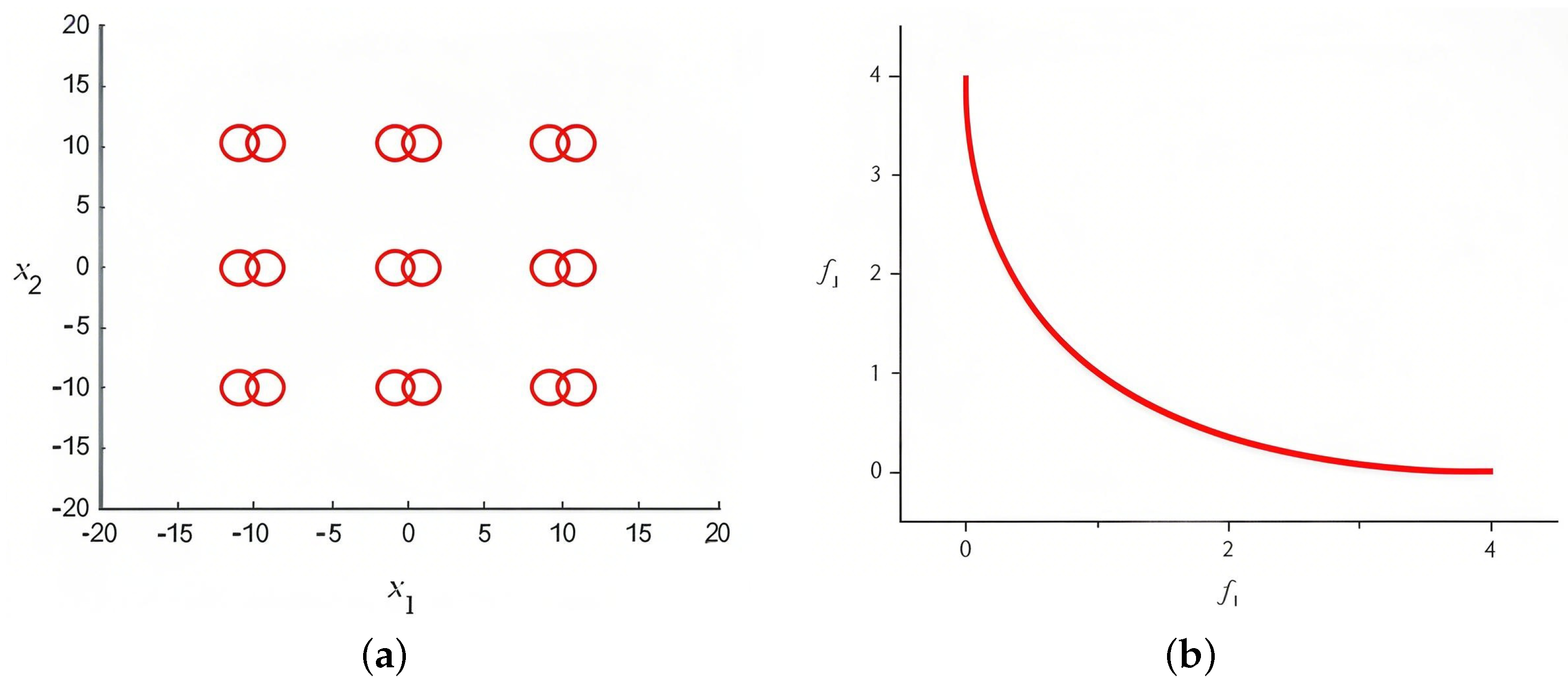
Multimodal multiobjective optimization problems (MMOPs) represent a distinctive class within the realm of multiobjective optimization, aiming to provide decision-makers with all the optimal solutions [2]. An MMOP is characterized by having different decision vectors corresponding to the same objective vector. Due to the potential equality of objective vectors for different solutions, an MMOP may exhibit multiple Pareto sets associated with a single Pareto front, as illustrated in Figure 1. The challenge in solving MMOPs lies in determining the Pareto front and identifying all the Pareto sets corresponding to it. This endeavor is crucial in providing decision-makers with a comprehensive set of optimal solutions [3]. However, focusing solely on global optima and neglecting local optima may result in decision-makers lacking a holistic understanding of the problem [4,5]. In situations where attaining any global optimum becomes impractical for decision-makers, the consideration of local optima becomes essential.

Algorithms for solving MMOPs with local Pareto fronts necessitates obtaining all global optima and securing high-quality local optima to address the intricacies of real-world scenarios. In MMOPs, there may also be a special case where the objective vectors of two distinct solutions, although different, are closely related. For instance, consider the following two solutions and their corresponding objective vectors:

$$\begin{array}{cc}\hfill {\mathbf{x}}_{\mathbf{1}}=(1200,900)& \mathbf{F}\left({\mathbf{x}}_{\mathbf{1}}\right)=(100,90)\hfill \\ \hfill {\mathbf{x}}_{\mathbf{2}}=(200,100)& \mathbf{F}\left({\mathbf{x}}_{\mathbf{2}}\right)=(100,85)\hfill \end{array}$$

(3)

It can be observed that ${\mathbf{x}}_{\mathbf{1}}$ and ${\mathbf{x}}_{\mathbf{2}}$ differ significantly, but their corresponding objective vectors $\mathbf{F}\left({\mathbf{x}}_{\mathbf{1}}\right)$ and $\mathbf{F}\left({\mathbf{x}}_{\mathbf{2}}\right)$ are very close. Although ${\mathbf{x}}_{\mathbf{2}}$ is dominated by ${\mathbf{x}}_{\mathbf{1}}$, $\mathbf{F}\left({\mathbf{x}}_{\mathbf{2}}\right)$ is only slightly inferior to $\mathbf{F}\left({\mathbf{x}}_{\mathbf{1}}\right)$. 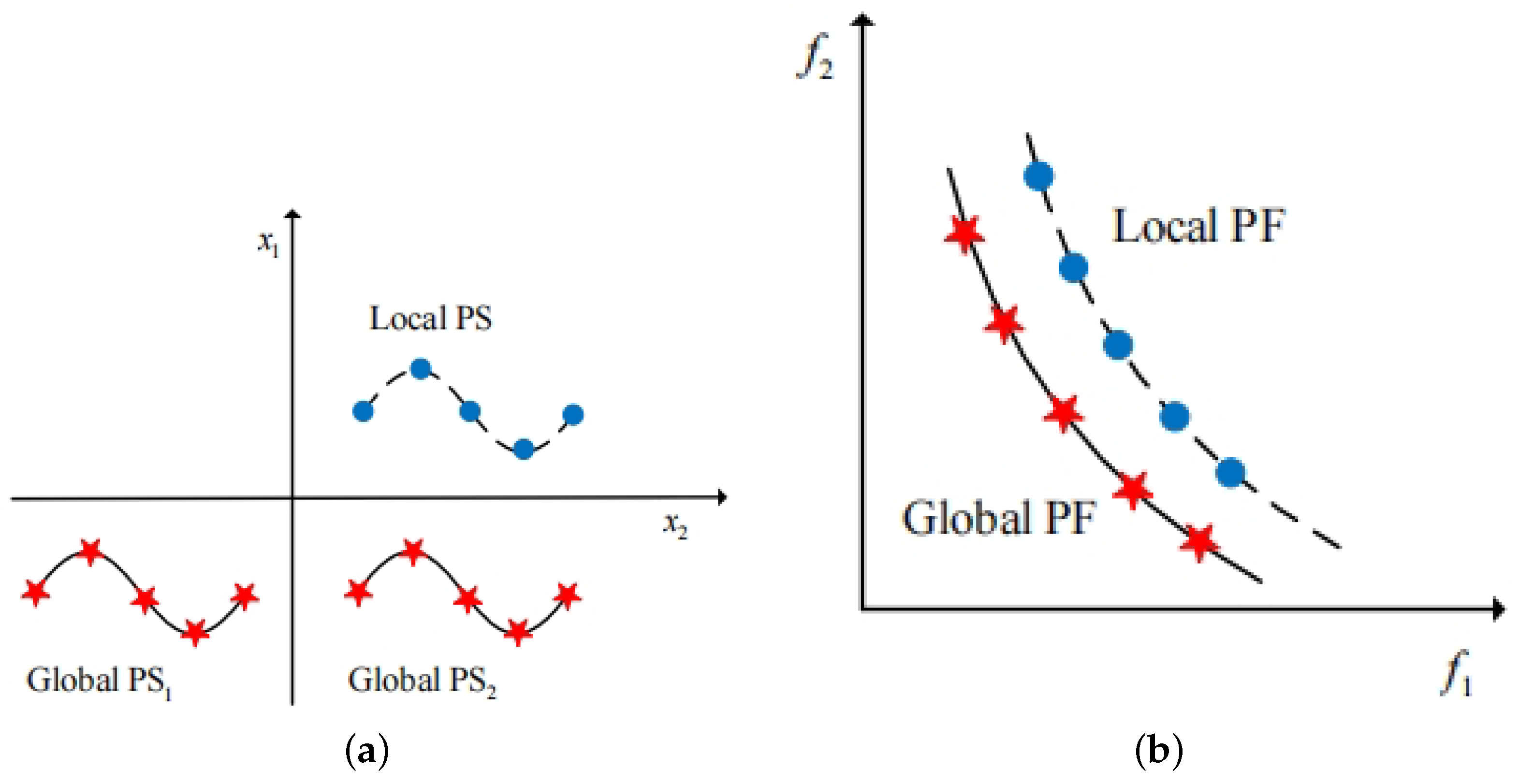In many cases, ${\mathbf{x}}_{\mathbf{2}}$ remains meaningful to the decision-maker since, when achieving ${\mathbf{x}}_{\mathbf{1}}$ is challenging, ${\mathbf{x}}_{\mathbf{2}}$ can be a viable alternative, given their small differences. In a multimodal multiobjective optimization problem, there may be multiple solutions resembling the relationship between ${\mathbf{x}}_{\mathbf{1}}$ and ${\mathbf{x}}_{\mathbf{2}}$—solutions that form distinct Pareto sets in the decision space and mutually dominating Pareto fronts in the objective space, as depicted in Figure 2. In this figure, the blue and red Pareto sets are distant in the decision space, but their corresponding Pareto fronts in the objective space are close. The solutions within the blue Pareto set are not dominated by any other solutions within their own neighborhood but are dominated by solutions in the red Pareto set. Therefore, the solutions in the blue Pareto set represent local optimal solutions, forming a set known as the local Pareto set (local PS), and their corresponding Pareto front is termed the local Pareto front (local PF). The solutions in the red Pareto set are global optimal solutions that are not dominated by any other solutions. They constitute the global Pareto set (global PS), with their corresponding Pareto front being the global Pareto front (global PF).

While solutions in the local Pareto set are dominated by solutions in the global Pareto set, their corresponding objective vectors differ only slightly. Additionally, solutions in the local Pareto set are not dominated by any other solutions within their own neighborhood. When decision-makers struggle to obtain global Pareto solutions, local Pareto solutions may serve as viable alternatives due to their proximity and slight inferiority to global optima [6]. Acquiring both global and local Pareto sets in MMOPs can provide decision-makers with diverse options for complex real-world scenarios. However, global Pareto fronts may significantly outperform local optima in objective space, rendering the latter irrelevant to decision-makers in some cases. Consequently, the problem may lack a local Pareto set and local Pareto front, featuring only the global Pareto set and global Pareto front. This paper will focus on solving both local and global Pareto sets, proposing an adaptive microscale searching algorithm to address problems with and without local Pareto sets.

Most algorithms for solving MMOPs cannot detect local Pareto sets. Algorithms capable of finding local Pareto sets exhibit poor performance on problems lacking such sets. Researchers often employ evolutionary algorithms for MMOPs and MOPs because they can search decision spaces rapidly without requiring objective function expressions. Multiobjective evolutionary algorithms (MOEAs) for MOPs select top-performing solutions in objective space and retain them for subsequent searches, aiming to converge quickly to the Pareto front. However, conventional MOEAs lack mechanisms to preserve solution diversity, making them potentially unable to find all Pareto sets of MMOPs [3].

Multimodal multiobjective evolutionary algorithms (MMOEAs) for MMOPs use diversity-preserving mechanisms to retain all Pareto sets across the Pareto front. Examples include TriMOEA-TA&R [7], DN-NSGA-II [2], MO_Ring_PSO_SCD [8], and MMODE_ICD [9], which employ various mechanisms to preserve solution diversity. MMODE_ICD prioritizes solutions with lower decision-space crowding distance to preserve diversity but favors global Pareto sets over local ones, thus only identifying global Pareto fronts. Similar limitations affect other algorithms in detecting local Pareto sets/fronts [4,10].

There are few algorithms capable of finding local Pareto fronts, with MMOEA/DC [11] and HREA [12] being notable examples. These algorithms can find both the global and local Pareto sets of MMOPs. However, they exhibit poor objective-space convergence on problems without local Pareto fronts. While HREA shows strong decision-space convergence and diversity in such cases, its objective-space performance lags behind DN-NSGA-II and MMODE_ICD due to its complex local-Pareto-preserving selection mechanism, which hinders elimination of local optima. MMOEA/DC also underperforms due to slow objective-space convergence.

In summary, current algorithms for solving multimodal multiobjective optimization problems can be broadly categorized into two types. One type is capable of finding only the global Pareto front and not the local Pareto front, while the other can simultaneously find both the global and local Pareto fronts. However, the latter type tends to exhibit suboptimal performance in the objective space when solving problems without local Pareto fronts. The primary distinction between these two types of algorithms lies in their selection strategies. Algorithms unable to find local Pareto fronts select the current global optimum, aiming for rapid convergence to the global Pareto front. In contrast, Algorithms targeting local Pareto fronts prioritize local solutions over global optima, ensuring their discovery but slowing non-Pareto solution elimination. This is particularly problematic in problems without local Pareto fronts, where selecting local optima delays convergence. The effectiveness of such strategies hinges on the problem’s local Pareto structure; pre-determining their existence would allow adaptive strategy adjustment, unlike fixed-strategy algorithms. Thus, a method to detect local Pareto fronts is essential.

In order to effectively solve multimodal multiobjective optimization problems with and without local Pareto fronts, we have devised the microscale searching multimodal multiobjective evolutionary algorithm (MMOEA_MS). Our observation suggests that algorithms capable of solving local Pareto fronts yield solutions in the early iterations, which can reflect the distribution of solutions in the objective space and indicate the presence or absence of local Pareto fronts. Consequently, a convolutional neural network is designed to extract information about the distribution of solutions in the objective space, enabling the detection of the existence of local Pareto fronts. Based on the presence or absence of local Pareto fronts, we can adjust the algorithm’s selection strategy, allowing it to search within the region where the Pareto set exists (valid decision subset). This type of algorithm, which determines the search space before solving, is referred to as a microscale searching algorithm [13,14]. When applied to multiobjective evolutionary algorithms, it is termed the microscale searching multimodal multiobjective evolutionary algorithm (MMOEA_MS).

In contrast to other algorithms, MMOEA_MS does not predefine a search strategy before solving; instead, it formulates a strategy based on the current problem’s local Pareto fronts and proceeds with the solution. When solving problems without local Pareto fronts, MMOEA_MS searches around the current optimal solutions and their neighborhoods, while it focuses on the local optimal solutions and their neighborhoods when local Pareto fronts are present. This capability is primarily attributed to the neural networks for detecting local Pareto fronts.

The structure of this paper is outlined as follows. In Section 2, we categorize multimodal multiobjective evolutionary algorithms into two types: those incapable of solving local Pareto fronts and those capable of doing so. The two categories are analyzed in detail. Section 3 is a pivotal section where a neural network-based method for detecting local Pareto fronts is introduced, laying the foundation for the subsequent development of a comprehensive algorithm. In Section 4, we present the microscale searching multimodal multiobjective evolutionary algorithm based on the detection of local Pareto fronts. This section covers the algorithmic framework and distinctive features of MMOEA_MS. In Section 5, MMOEA_MS is applied to solve problems with and without local Pareto fronts. We compare the results with other state-of-the-art algorithms and provide an analysis of the experimental outcomes. Finally, in Section 6, we conclude our research work, summarizing the key findings, and initiate a discussion on future research directions.

2. Related Works

Algorithms for solving multimodal multiobjective optimization problems can be categorized into two types: one capable of finding only the global Pareto set, and the other able to identify both the global and local Pareto sets. In this section, we will introduce and analyze these two types of algorithms separately.

2.1. Evolutionary Algorithms for Solving MMOPs Without Local Pareto Fronts

Crowding distance is widely used in MMOP algorithms to identify Pareto sets. NSGA-II [15] uses crowding distance to evaluate non-dominated solutions, selecting those with larger objective-space distances to maintain diversity. Unlike NSGA-II (which focuses solely on objective-space diversity), Omni-optimizer [16,17] considers crowding distance in both decision and objective spaces, enabling it to detect multiple global Pareto sets. DN-NSGA-II and MMODE_ICD instead use decision-space Euclidean distance for diversity retention: DN-NSGA-II calculates pairwise Euclidean distances, while MMODE_ICD employs weighted sums of neighborhood Euclidean distances and prioritizes less crowded solutions during selection. This dual focus on decision/objective space density makes MMODE_ICD more effective at identifying all global Pareto sets.

In addition to crowding distance, many algorithms for solving MMOPs also utilize niching techniques to maintain diversity in the decision space. Niching techniques have gained widespread popularity in recent years for solving MMOPs, primarily involving the decomposition of the entire population into multiple niches. Within each niche, some information can be shared, and the algorithm iteratively solves each niche separately to maintain overall population diversity [18,19]. Before employing crowding distance for environmental selection, DN-NSGA-II divides the overall population into multiple niches. MO_Ring_PSO_SCD uses index-based ring topology and dual-space crowding distance to maintain niche diversity. LBPDADE [20,21] employs LBP-based adaptive differential evolution to form niches, with individuals mutating using global/local niche information. NMOHSA [22] leverages neighborhood-based dynamic memory and creative rules to avoid local optima. While niching techniques preserve decision-space diversity, DN-MMOES [23] addresses density imbalance via two-stage niching (decision space first, then dual spaces). NCD-DE [18] optimizes niche generation by pre-searching centers. Xiaodong Li et al. [24,25] summarize that niching enhances MMOP performance by partitioning populations to retain diversity and identify global Pareto sets. For problems without local Pareto fronts, FBK-DE [26] uses NBC clustering to balance subpopulation sizes and preserve decision-space diversity. TriMOEA-TA&R [7] employs dual archives (diversity via clustering/niching, convergence to global front) for MMOPs. DSCPSO-EMM [27,28] uses clustering to detect global Pareto sets in expensive multimodal problems.

2.2. Evolutionary Algorithms for Solving MMOPs with Local Pareto Fronts

While there are many multimodal multiobjective optimization algorithms capable of solving MMOPs, they typically select the optimal solutions during environmental selection. This practice hinders the preservation of local optimal solutions, preventing the algorithm from identifying the local Pareto sets for the current problem. Therefore, to successfully find the local Pareto fronts, algorithms should refrain from exclusively selecting the current optimal solutions.

Algorithms designed to solve problems with local Pareto fronts employ various strategies to retain local optimal solutions and discover the corresponding local Pareto sets. For instance, DNEA-L enhances the DNEA algorithm by introducing an update method for a multiple Pareto front archive to identify local Pareto sets for specific problems [29,30,31]. The algorithm is effective in solving for local Pareto sets in certain scenarios. CEA-LES employs a layer-to-layer evolution strategy to evolve equivalent global and local Pareto sets, successfully solving for local Pareto fronts [32]. MMOGA facilitates evolution in local regions by only comparing solutions within the same ecological niche, leading to the discovery of local optimal solutions and local Pareto sets for the current problem [33]. ${\mathrm{I}}_{LC}$-MMEA improves the environmental selection strategy by introducing a local convergence index, ultimately searching for both global and local Pareto sets [4]. MMOEA_DC utilizes a dual clustering approach, dividing the population into multiple subpopulations in both decision and objective spaces for iterative solving. Unlike niche techniques, MMOEA_DC performs environmental selection only within each subpopulation, achieving the solution of both global and local optimal solutions. HREA hierarchically organizes solutions in the objective space and conducts independent environmental selection on each layer. This strategy ensures that environmental selection occurs locally rather than globally, facilitating the discovery of local Pareto sets. Therefore, HREA is adept at solving local Pareto sets [34,35].

2.3. Analysis of the Two Types of Algorithms

Algorithms for problems without local Pareto fronts prioritize decision-space solution diversity. In MMOPs, selecting solely based on objective-space optimality may miss global Pareto sets, as identical objective vectors can mask distinct solutions. Thus, these algorithms incorporate metrics like crowding distance into environmental selection, balancing objective performance with diversity to prevent unimodal convergence [18]. For problems with local Pareto fronts, algorithms focus on preserving local optima. Such problems require higher solution diversity due to coexisting global/local Pareto sets. While crowding distance aids diversity, dominance of global over local solutions necessitates subpopulation partitioning: environmental selection within niches prevents local optima elimination, enabling discovery of local Pareto sets [11].

The main distinction between evolutionary algorithms designed to solve problems with and without local Pareto fronts lies in the choice made during environmental selection—whether to select the current global optimal solutions or the local optimal solutions. As both types of algorithms aim to maintain solution diversity, they employ criteria beyond the performance of the objective vectors as references during environmental selection. Additionally, various techniques are utilized to ensure a rich diversity of solutions in the decision space. The primary difference between the two types of algorithms lies in the selection of either the current global optimal solutions or the local optimal solutions. Algorithms designed for problems without local Pareto fronts tend to select the current global optimal solutions during environmental selection. This allows them to rapidly search for the global Pareto set while maintaining solution diversity. However, they are unable to discover local Pareto sets. On the other hand, algorithms designed for problems with local Pareto fronts tend to select local optimal solutions. This approach maximizes the preservation of solution diversity, preventing the neglect of local optimal solutions within local Pareto sets.

Both algorithm types perform well on their target problems but struggle with other problem types. We find that identifying whether local Pareto fronts exist allows algorithms to adapt their selection strategies. To address this, we introduce a local Pareto front detection method and propose an algorithm capable of solving both problem types based on this detection.

3. Local Pareto Front Detection Based on Neural Network Classifier

Evolutionary algorithms employ distinct strategies when solving problems with and without local Pareto fronts. When addressing problems lacking local Pareto fronts, the algorithms typically opt to retain the global optimal solution at each iteration to swiftly explore the entire Pareto set. In contrast, when addressing problems with local Pareto fronts, the evolutionary algorithms prioritize preserving the local optimal solutions at each iteration to maintain the local Pareto set. However, during practical problem-solving, the algorithms struggle to ascertain the presence of local Pareto fronts, resulting in the potential inadequacy of the chosen strategies for finding the Pareto set. If the existence of local Pareto fronts could be determined beforehand, it would enable the algorithms to adapt their strategies based on the specific circumstances of the problem. This section introduces the characteristics of local Pareto fronts in the objective space and a neural network classifier designed based on these characteristics. This classifier aims to detect whether the current problem has the local Pareto front.

3.1. Characteristics of Local Pareto Fronts in the Objective Space

Algorithmic selection strategies differ between solving problems with and without local Pareto fronts. The local Pareto sets provide decision-makers with more selectable solutions. Due to the dominance of the global Pareto front over the local Pareto front, adopting a strategy of selecting the global optimal solutions may hinder the algorithms from retaining the local Pareto set throughout iterations. Although the fitness values of the local Pareto front may slightly lag behind those of the global Pareto front, solutions within the local Pareto set exhibit optimal performance within their respective neighborhoods [12]. Therefore, when solving problems with local Pareto fronts, evolutionary algorithms tend to select local optimal solutions in the hope of preserving all Pareto sets for the current problem. Individuals distant from true Pareto sets may still be locally optimal within their neighborhoods, and local optimal selection may fail to remove them, slowing the search. Conversely, current optimal selection rapidly eliminates such outliers. Thus, for problems without local Pareto fronts, algorithms should prioritize current optimal individuals. Pre-detecting local Pareto fronts allows evolutionary algorithms to adaptively choose between current or local optimal selection strategies.

The distribution of solutions in the objective space can be leveraged to determine the presence of a local Pareto front in the current problem. In the context of multimodal multiobjective optimization problems, where different solutions may have identical objective function values, the true Pareto sets in the decision space for problems with and without local Pareto fronts may be highly similar, as illustrated in Figure 3. This implies that the distribution of solutions in the decision space for problems with and without local Pareto fronts may be very similar and challenging to differentiate. In contrast to problems without local Pareto fronts, problems with local Pareto fronts exhibit multiple true Pareto curves or surfaces in the objective space, where the local Pareto fronts are dominated by the global Pareto front, as depicted in Figure 4. Comparing Figure 3 and Figure 4, it becomes evident that the local Pareto front can be clearly distinguished from the global Pareto front, while the differences between local and global Pareto sets are less pronounced. Therefore, the information from the objective space can be utilized to discern the presence of a local Pareto front in the current problem.

3.2. Network Model Design for Local Pareto Front Detection

Observations indicate that algorithms capable of solving problems with local Pareto fronts, such as MMOEA/DC and HREA, exhibit a convergence of solution distributions in the objective space towards the true Pareto fronts of the current problem gradually over iterations, encompassing both the global and local Pareto fronts, as illustrated in Figure 5. This indicates that the distribution of solutions in the objective space obtained in the early iterations may already provide insights into the existence of local Pareto fronts in the current problem. Based on this assumption, we have devised a classifier to detect the presence or absence of local Pareto fronts in the current problem. The classifier takes the distribution of solutions in the objective space as input, which is obtained by algorithms capable of solving problems with local Pareto fronts in the first n iterations on the current problem. The output is the classification of the current problem into categories based on the presence or absence of local Pareto fronts.

The distribution of solutions in the objective space can be represented as a binary matrix, where each solution corresponds to a non-zero element in the matrix. Due to the dominance of the global Pareto front over the local Pareto front, the local Pareto front is farther from the origin in the objective space than the global Pareto front. In Figure 5, solutions near the local Pareto front are also farther from the origin in the objective space than those near the global Pareto front. This feature can be expressed using contextual information from the objective space. Convolutional operations can extract contextual information from the objective space, capturing the local semantics of whether a Pareto front is farther from the origin in the objective space compared to the global Pareto front. Therefore, this approach utilizes convolution to extract contextual information about the distribution of solutions in the objective space to detect the presence of local Pareto fronts in the current problem. To facilitate convolution operations in the objective space, this method represents the distribution of solutions in the objective space as a binary matrix, where each solution corresponds to a non-zero element in the matrix. The definition of each solution to be represented is as follows:

$$\begin{array}{cc}\hfill s& =[i,\mathbf{F}]\hfill \\ \hfill \mathbf{F}& =[f_1,f_2,\dots ,f_m]\hfill \end{array}$$

(4)

where s is a solution, i is the current iteration count, $\mathbf{F}$ is the objective vector corresponding to the solution, $f_j$ is the value of the solution on the j-th objective function, and m is the number of objective functions in the current problem. As the determination of the presence of local Pareto fronts relies solely on the distribution in the objective space, the solutions to be represented do not include the values of decision variables.

The algorithm for transforming the distribution of solutions in the objective space into a binary matrix is presented in Algorithm 1. Algorithm 1 normalizes the objective function values of the solutions and stretches them to the specified size of the matrix, denoted as $size$ (lines 4–8). This conversion maps the objective function values of solutions to the corresponding elements’ coordinates in the matrix, achieving a mapping from solutions in the objective space to non-zero elements in the matrix. It also ensures that the distribution of solutions in the objective space for different problems can be represented by matrices of the same size. In the resulting binary matrix, each non-zero element represents a solution in the objective space, while zero elements indicate the absence of solutions at the corresponding positions in the objective space (lines 9–11). It is noteworthy that the matrix’s dimension is one more than the objective space’s dimension because the matrix also needs to record the iteration count for each solution. The obtained binary matrix can be used to train a convolutional neural network classifier.

The network architecture of the classifier is depicted in Figure 6, comprising multiple convolutional layers and fully connected layers. The multilayer convolution facilitates the extraction of contextual information from the matrix, namely the contextual information of the solutions’ distribution in the objective space. Subsequently, the fully connected layers enable the mapping of contextual information to the presence or absence of a local Pareto front. In Figure 5, the initially retained distribution of solutions in the objective space exhibits some randomness, making it challenging to discern the presence of a local Pareto front based on these solutions. Only after a certain number of iterations can the distribution of retained solutions in the objective space reflect whether the current problem has a local Pareto front. Consequently, the impact of solution distributions at different stages on the classification varies. Exploiting this phenomenon, the designed convolutional network first trains a weight vector and multiplies it with the input matrix before proceeding with subsequent operations. For evolutionary algorithms, the role of the weight vector is to determine how much the solutions at different iteration affect the judgment of whether a local Pareto front exists. In summary, the designed network can extract contextual information from the distribution of solutions in the objective space to ascertain the presence of local Pareto fronts in the current problem. The complete structure of the network is illustrated in Figure 7.

3.3. Network Training for Local Pareto Front Detection

As illustrated in Figure 5, when MMOEA/DC and HREA solve MMOPs, the early-stage distribution of solutions in the objective space already manifests whether the current problem has a local Pareto front. Therefore, these two algorithms can be employed to iterate n times on the current problem, considering the distribution of solutions in the objective space obtained during the iteration process as training data for the network model. Due to the inherent randomness in the initialization of evolutionary algorithm populations, solving the same problem multiple times using the same algorithm results in different solutions. Repeatedly applying these algorithms to solve problems known to have or lack local Pareto fronts can get abundant labeled training data. Algorithm 1 represents the distribution of solutions in the objective space using matrices, including the normalization of values for each coordinate of the objective vector. The normalization operation is influenced by outliers, leading to uneven distribution of non-zero elements in the transformed matrix. Therefore, it is necessary to remove outliers in the objective space, and the algorithm for removing outliers is outlined in Algorithm 2. Algorithm 2 achieves outlier removal by eliminating solutions with objective function values significantly greater or smaller than the mean. For evolutionary algorithms, this is akin to disregarding individuals far from the population, preventing outliers from causing an uneven distribution in the population.

The training of the network model can commence after obtaining rich training data and pre-processing it by using Algorithms 1 and 2 sequentially. To prevent overfitting during the training process, the dataset is divided into a training set, validation set, and test set. Training is halted when the model’s performance on the validation set does not improve continuously for multiple iterations. As the proposed network model is essentially a classifier, cross-entropy is employed as the loss function during training to assess the current model’s performance.

Algorithm 1 Matrix Representation of Solution Distribution in Objective Space.

Input: $S=[s_1,s_2,\dots ,s_M]$: Solutions retained after the i-th iteration, where $s_j$ represents the j-th solution and M represents the number of retained solutions. $size$: The size of the matrix to be transformed. $p_{val}$: The value of non-zero elements in the transformed matrix. Output: $tranMatrix$, The transformed matrix. 1: Initialize $tranMatrix$ 2: for $j\leftarrow 0$ to m do 3:      $va{l}_{max}\left[j\right]\leftarrow$ the maximum value of the j-th objective function in S 4:      $va{l}_{min}\left[j\right]\leftarrow$ the minimum value of the j-th objective function in S 5: end for 6: for $l\leftarrow 1$ to $m+1$ do 7:      $S[:,l]\leftarrow {\displaystyle \frac{S[:,l]-va{l}_{min}[l-1]}{va{l}_{max}[l-1]-va{l}_{min}[l-1]}}\times size$ 8: end for 9: for $k\leftarrow 0$ to M do 10:      $tranMatrix\left[S[k,1],S[k,2],\dots ,S[k,m],S[k,0]\right]\leftarrow p_{val}$ 11: end for 12: return $tranMatrix$

Algorithm 2 Outlier Removal.

Input: $S=[s_1,s_2,\dots ,s_M]$: Solutions retained after the i-th iteration, where $s_j$ represents the j-th solution and M represents the number of retained solutions. Output: S: Solutions after Outlier Removal 1: Initialize $va{l}_{max},va{l}_{min},va{l}_{mean},va{l}_{std}$ 2: for $j\leftarrow 0$ to m do 3:      Calculate the maximum value $va{l}_{max}$, minimum value $va{l}_{min}$, mean $va{l}_{mean}$, and standard deviation $va{l}_{std}$ of the j-th objective function $f_j$ in S. 4:      while $va{l}_{max}>va{l}_{mean}+3\times va{l}_{std}$ or $va{l}_{min}<va{l}_{mean}-3\times va{l}_{std}$ do 5:          Remove the solutions corresponding to $va{l}_{max}$ and $va{l}_{min}$ from S. 6:          Recalculate the maximum value $va{l}_{max}$, minimum value $va{l}_{min}$, mean $va{l}_{mean}$, and standard deviation $va{l}_{std}$ of the j-th objective function $f_j$ in S. 7:      end while 8: end for 9: return S

4. Adaptive Microscale Searching Algorithm Based on Pre-Trained Network

Evolutionary algorithms are supposed to employ different strategies to solve problems with and without local Pareto fronts. The choice of strategy fundamentally influences the algorithm by determining distinct search scopes. An appropriate search scope should encompass all Pareto sets and have a significantly smaller scale than the entire decision space. A search scope like this represents the valid decision subset of the current problem. Utilizing the pre-trained neural network model, evolutionary algorithms can first determine the presence of a local Pareto front in the current problem and select an appropriate strategy to determine the search scope of the problem. Consequently, evolutionary algorithms estimate the valid decision subset for the current problem through the pre-trained model. Building upon the pre-trained network capable of detecting the existence of local Pareto fronts, this section introduces the adaptive microscale searching algorithm for solving multimodal multiobjective optimization problems.

4.1. Microscale Searching Assumptions for Multimodal Multiobjective Optimization Problems

Evolutionary algorithms require iterative mutation and selection operations to gradually search Pareto sets in the decision space. The region where the Pareto sets reside is relatively small compared to the entire decision space, necessitating multiple iterations for the algorithm to find the Pareto sets. If the evolutionary algorithm can focus its search within a subset that contains the Pareto set, the task of mutation-based searching becomes more manageable. This subset smaller than the entire decision set is referred to as the decision subset, and one that encompasses the Pareto set is termed a valid decision subset. Efficient allocation of computational resources is crucial for enhancing the search efficiency, with the algorithm primarily concentrating its computational resources on the valid decision subset. Algorithms that first determine the valid decision subset and allocate computational resources based on the valid decision subset are termed microscale searching algorithms.

When solving problems with and without local Pareto fronts, evolutionary algorithms are supposed to explore different search spaces. In the context of multimodal multiobjective optimization problems, where multiple Pareto sets correspond to a single Pareto front, algorithms search in the neighborhoods of all current optimal solutions. However, when dealing with problems with local Pareto fronts, searching in the neighborhoods of the current optimal solutions may fail to find the local Pareto set. Consequently, algorithms tend to opt for searches around local optimal solutions to find all Pareto sets in problems with local Pareto fronts. Local optimal solutions include the current optimal solutions and additional non-current optimal local solutions. This results in the size of the neighborhoods around local optimal solutions being much larger than those around the current optimal solutions. When solving problems without local Pareto fronts, choosing to search around local optimal solutions and their neighborhoods would waste computational resources because the Pareto sets are concentrated around the current optimal solutions and their neighborhoods. Therefore, algorithms should adapt their search spaces based on the presence of local Pareto fronts. When without local Pareto fronts, the algorithm’s search space should be around the current optimal solutions and their neighborhoods. Otherwise, computational resources would be wasted by searching in the neighborhoods of non-current optimal local solutions. This explains why MMOEA/DC and HREA may not perform well on problems without local Pareto fronts.

It is essential to determine the valid decision subset of the current problem before initiating the search. The mutation and selection operations of evolutionary algorithms typically operate within the solutions retained from the previous iteration and their neighborhoods. Consequently, the decision subset determined by evolutionary algorithms consists of the solutions retained from each iteration and their respective neighborhoods. However, the decision subset determined by the algorithm is not necessarily the valid decision subset for the current problem. For instance, in the case of MMOEA_ICD solving problems with local Pareto fronts, the determined search space is around the current optimal solutions and their neighborhoods, neglecting the local optimal solutions and their neighborhoods. This oversight could result in the algorithm eliminating solutions within the local Pareto set during the iteration process, leading to the failure to solve the local Pareto set. Therefore, when solving multimodal multiobjective optimization problems, evolutionary algorithms need to first determine the valid decision subset of the current problem.

4.2. Valid Decision Subset for Multimodal Multiobjective Optimization Problems

Evolutionary algorithms solving MMOPs apply mutation operations to individuals in the population and select individuals that meet certain criteria from both the mutated and original individuals to be retained. Each mutation is based on the individuals retained from the previous iteration. This implies that evolutionary algorithms do not search the entire decision space but rather explore the neighborhoods of the retained individuals. Therefore, the decision subset determined by evolutionary algorithms consists of the retained individuals and their neighborhoods. However, the distribution of Pareto sets for problems with and without local Pareto fronts differs. The decision subset identified by evolutionary algorithms may not be the valid decision subset for the current problem. This section will analyze the valid decision subset for problems with and without local Pareto fronts.

4.2.1. Valid Decision Subset for Problems Without Local Pareto Fronts

In problems without local Pareto fronts, there are only global Pareto sets, implying that no solution in the Pareto sets is dominated by any other solution. Therefore, when solving problems without local Pareto fronts, the algorithm should select the current optimum individuals to be retained. This approach enables a quick search for the Pareto sets. Due to the presence of multiple Pareto sets in MMOPs, relying solely on objective function values as a selection criterion makes it challenging for the algorithm to find all Pareto sets. Therefore, some algorithms, such as MMODE_ICD, also consider crowding distance [9]. Regardless of the selection criterion chosen, selecting the current optimum individuals facilitates a faster discovery of the Pareto sets when solving MMOPs without local Pareto fronts. The valid decision subset for MMOPs without local Pareto fronts is the optimum individuals and their neighborhoods at each iteration. This is mathematically defined as follows:

$$\begin{array}{cc}\hfill \mathbf{F}\left(\mathbf{x}\right)& =(f_1\left(\mathbf{x}\right),\dots ,f_m\left(\mathbf{x}\right))\hfill \\ \hfill {\mathbf{X}}_{\mathbf{Goptim}}& =\left\{\mathbf{x}\right|\mathbf{f}\left(\mathbf{x}\right)\le \mathbf{f}\left(\mathbf{z}\right),\forall \mathbf{z}\in \mathbf{X}\}\hfill \\ \hfill {\mathbf{X}}_{\mathbf{Gvds}}& =\left\{\mathbf{x}\right||\mathbf{x}-\mathbf{a}|\le \sigma ,\exists \mathbf{a}\in {\mathbf{X}}_{\mathbf{Goptim}}\}\hfill \end{array}$$

(5)

where $\mathbf{F}\left(\mathbf{x}\right)$ is all objective functions, $\mathbf{X}$ is the entire decision set, ${\mathbf{X}}_{\mathbf{Goptim}}$ are the current optimum solutions, $\sigma$ is a small constant indicating the neighborhood of the current optimal solution and ${\mathbf{X}}_{\mathbf{Gvds}}$ is the valid decision subset for problems without local Pareto fronts.

4.2.2. Valid Decision Subset of Problems with Local Pareto Fronts

The Pareto sets for problems with local Pareto fronts encompasses both the global Pareto sets and the local Pareto set, where solutions within the local Pareto set are dominated by those within the global Pareto sets. Consequently, selecting the current optimum individuals during the solving process would be inadequate for preserving the local Pareto set. Algorithms capable of solving the local Pareto set need to search within the neighborhood of local optimal solutions. MMOEA/DC achieves this through cluster-based selection of local optimal solutions [11], while HREA employs a hierarchical approach for selecting local optimal solutions [12]. Despite the different strategies employed by these algorithms, the retained local optimal solutions ultimately help the algorithm in finding the local Pareto set. This is because the fact that solutions within the local Pareto set exhibit superior performance within their respective neighborhoods [12]. Therefore, the valid decision subset for multimodal multiobjective optimization problems with local Pareto fronts is defined as the local optimum solutions and their neighborhoods at each iteration. This is mathematically defined as follows:

$$\begin{array}{cc}\hfill \mathbf{F}\left(\mathbf{x}\right)& =(f_1\left(\mathbf{x}\right),\dots ,f_m\left(\mathbf{x}\right))\hfill \\ \hfill {\mathbf{X}}_{\mathbf{Loptim}}& =\left\{\mathbf{x}\right|\mathbf{f}\left(\mathbf{x}\right)\le \mathbf{f}\left(\mathbf{z}\right),\forall \mathbf{z}|\mathbf{z}-\mathbf{x}|\le \lambda \}\hfill \\ \hfill {\mathbf{X}}_{\mathbf{Lvds}}& =\left\{\mathbf{x}\right||\mathbf{x}-\mathbf{a}|\le \sigma ,\exists \mathbf{a}\in {\mathbf{X}}_{\mathbf{Loptim}}\}\hfill \end{array}$$

(6)

where $\mathbf{F}\left(\mathbf{x}\right)$ is all objective functions, $\mathbf{X}$ is the entire decision set, ${\mathbf{X}}_{\mathbf{Loptim}}$ are the local optimum solutions, and $\sigma$ and $\lambda$ are small constants used to denote the neighborhood of the local optimum. ${\mathbf{X}}_{\mathbf{Lvds}}$ is the valid decision subset for problems with local Pareto fronts.

4.3. Valid Decision Subset Estimation Based on Pre-Trained Network

The valid decision subset for multimodal multiobjective problems can be estimated by using the pre-trained network. The presence or absence of local Pareto fronts directly impacts the valid decision subset of the current problem. If an algorithm can ascertain the existence of local Pareto fronts, it is possible to determine the valid decision subset of the current problem. The pre-trained network model introduced in the preceding sections can detect the presence of local Pareto fronts in the current problem, thereby enabling the determination of the valid decision subset. The algorithm for estimating the valid decision subset based on the pre-trained network is outlined in Algorithm 3.

Algorithm 3 Estimation of the Valid Decision Subset.

Input: $S=[s_1,s_2,\dots ,s_M]$: Solutions retained after the i-th iteration, where $s_j$ represents the j-th solution and M represents the number of retained solutions. $size$: The size of the matrix to be transformed. $p_{val}$: The value of non-zero elements in the transformed matrix. $model$: The pre-trained convolutional neural network model. $esti\text{\_}alg$: The estimation operator. n: Number of iterations for the estimation operator. Output: $select\text{\_}strategies$, the selection strategies appropriate for the current problem (selecting the local optimal solutions or the current optimal solutions in each iteration) 1: Initialize S, $input\text{\_}data$ 2: for $i\leftarrow 0$ to n do 3:       $S\leftarrow esti\text{\_}alg\left(S\right)$ 4:       $S\leftarrow \mathbf{Algorithm} \mathbf{2}\left(S\right)$//Remove outliers 5:       $input\text{\_}data\leftarrow input\text{\_}data+\mathbf{Algorithm} \mathbf{1}(S,size,p_{val})$//Convert the data into matrices as input for the model 6: end for 7: if  $model\left(input\text{\_}data\right)$  do 8:      $select\text{\_}strategies\leftarrow$ Select the local optimal solutions to be retained in each iteration, obtaining the valid decision subset as in Equation (6) 9: else do 10:      $select\text{\_}strategies\leftarrow$ Select the current optimal solutions to be retained in each iteration, obtaining the valid decision subset as in Equation (5) 11: end if 12: return  $select\text{\_}strategies$

Algorithm 3 initially employs the estimation operator to solve the current problem for a specified number of iterations, generating the iterated solutions and their corresponding objective vectors. Following the removal of outliers in the objective space using Algorithm 2, the distribution of solutions in the objective space is represented as a matrix using Algorithm 1, serving as input for the pre-trained model. The model outputs the category of the current problem, indicating the presence or absence of local Pareto fronts. Based on the model’s output, Algorithm 3 estimates the valid decision subset of the current problem, conforming to either (5) or (6). With the estimated valid decision subset, the algorithm adaptively adjusts the evolutionary algorithm’s selection strategy and allocates computational resources to the valid decision subset.

4.4. Computational Resource Allocation Rules for Local Pareto Fronts

The Pareto sets of multimodal multiobjective optimization problems are included in the valid decision subset. Therefore, the algorithm should allocate more computational resources to the valid decision subset. The estimation of the valid decision subset for multimodal multiobjective optimization problems with or without local Pareto fronts can be obtained through Algorithm 3. Based on the estimated valid decision subset, the algorithm can set the computational resource allocation rules. The main difference between the computational resource allocation rules for the two types of problems lies in whether they include non-current optimal local optima and their neighborhoods. Therefore, their computational resource allocation rules differ mainly in whether to allocate computational resources to non-current optimal local optima and their neighborhoods. Specifically, problems with local Pareto fronts require allocating the main computational resources to search in the neighborhood of local optimal solutions, while problems without local Pareto fronts require allocating the main computational resources to search in the neighborhood of the current optimal solutions. Their mathematical definitions are as follows:

$$powe{r}_{area}=\left\{\begin{array}{cc}{\mathbf{X}}_{\mathbf{Gvds}}\hfill & \mathrm{without}\mathrm{Local}\mathrm{Pareto}\mathrm{Fronts}\hfill \\ {\mathbf{X}}_{\mathbf{Lvds}}\hfill & \mathrm{with}\mathrm{Local}\mathrm{Pareto}\mathrm{Fronts}\hfill \end{array}\right.$$

(7)

where $powe{r}_{area}$ is the region of computational resource allocation, and ${\mathbf{X}}_{\mathbf{Gvds}}$ and ${\mathbf{X}}_{\mathbf{Lvds}}$ refer to the neighborhoods of the global optimal solutions as defined in Equation (5) and the local optimal solutions as defined in Equation (6), respectively.

In each iteration, evolutionary algorithms perform mutation and selection based on the individuals preserved from the last iteration and their neighborhoods. This set of preserved individuals and their neighborhoods is the decision subset determined by the evolutionary algorithm. The allocation of computational resources is reflected in the fact that mutation is carried out on the preserved individuals and their neighborhoods rather than randomly across the entire decision space. When solving problems without local Pareto fronts, the evolutionary algorithm should select the current optimal solutions and perform mutation in their neighborhoods. In contrast, when solving problems with local Pareto fronts, the evolutionary algorithm should select the local optimal solutions and perform mutation in their neighborhoods. In this way, the evolutionary algorithm achieves computational resource allocation.

4.5. Microscale Searching Algorithm Framework for Solving MMOPs

The microscale searching algorithm for solving MMOPs (MMOEA_MS) is presented. The framework of the microscale searching algorithm is illustrated in Algorithm 4. When using evolutionary algorithms to solve MMOPs, the number of iterations is generally fixed at N times. Since the estimation operator is applied to iterate n times on the current problem when detecting the local Pareto front, there are $N-n$ iterations left for the subsequent solution.

The key to the microscale searching algorithm lies in determining the valid decision subset and formulating the computational resource allocation rules, as explicitly visualized in Figure 8. In MMOEA_MS, the valid decision subset is estimated through the pre-trained model— a process depicted by the ’Neural Network Detection’ module in Figure 8b—and the computational resource allocation rules are formulated through different selection strategies (line 2). As shown in Figure 8a, the algorithm’s adaptive switching between MMODE_ICD and MMOEA/DC operators is governed by the detection of local Pareto fronts: the left branch of Figure 8a illustrates the use of MMODE_ICD for problems without local fronts, while the right branch highlights MMOEA/DC activation for problems with local fronts.

It is worth noting that the estimation of the valid decision subset (see the dashed box in Figure 8b) and the formulation of computational resource allocation rules are not implemented directly but achieved indirectly by adjusting mutation and selection operations—this is evident in Figure 8b’s ’Mutation-Selection Loop,’ where the green module ’Resource Allocation’ dynamically adjusts search scope based on operator selection. For instance, when MMOEA/DC is employed (right path in Figure 8), the algorithm allocates resources to local optimal solution neighborhoods, whereas MMODE_ICD focuses on global optima (left path). This adaptive mechanism, visualized in Figure 8’s hierarchical flow, underscores the framework’s capability to integrate diverse operators effectively.

Algorithm 4 MMOEA_MS’s Framework.

Input: $size$, The size of the matrix to be transformed. $p_{val}$: The value of non-zero elements in the transformed matrix. $model$: The pre-trained convolutional neural network model. $esti\text{\_}alg$: The estimation operator. N: Total number of iterations in the algorithm. n: Number of iterations for the estimation operator. Output: S, Solutions retained by the algorithm finally. 1: Initialize S 2: $select\text{\_}strategies\leftarrow$ $\mathbf{Algorithm} \mathbf{3}(S,size,p_{val},model,esti\text{\_}alg,n)$ 3: Initialize $\mathbf{mutate}, \mathbf{select}$ according to $select\text{\_}strategies$ 4: for $i\leftarrow n$ to N do 5:       $temp\leftarrow S+\mathbf{mutate}\left(S\right)$//Mutation 6:       $S\leftarrow \mathbf{select}(temp,select\text{\_}strategies)$//Selection 7: end for 8: return  S

5. Experiment

In order to validate the effectiveness of the proposed network-based algorithm for detecting local Pareto fronts and the microscale searching algorithm, we conducted relevant experiments. This section will introduce the designed experiments.

5.1. Experimental Settings

While there are numerous multimodal multiobjective optimization problems, those with local Pareto fronts are relatively scarce. This subsection will introduce the test problems chosen for this experiment and the metrics used to evaluate algorithm performance.

5.1.1. Selected Experimental Problems

The concept of local Pareto fronts was initially introduced in CEC 2019, where a problem set comprising twenty-two test problems was proposed. This problem set encompasses a variety of distributions and dimensions, featuring both problems with and without local Pareto fronts. Specifically, six of these problems involve local Pareto fronts. We selected these problem sets as the experimental testbed. Details of each problem in the set are provided in Table 1.

Table 1. The Details of the Problems.The problems of MMF10, MMF11, MMF12, MMF13, MMF15, and MMF15_a have a local Pareto front, while the remaining problems do not have local Pareto fronts.

Problem Name	Existence of Local Pareto Front
SYM-PART simple	✗
SYM-PART rotated	✗
Omni-test	✗
MMF1	✗
MMF1_z	✗
MMF1_a	✗
MMF2	✗
MMF3	✗
MMF4	✗
MMF5	✗
MMF6	✗
MMF7	✗
MMF8	✗
MMF9	✗
MMF10	✔
MMF11	✔
MMF12	✔
MMF13	✔
MMF14	✗
MMF14_a	✗
MMF15	✔
MMF15_a	✔

Table 1. The Details of the Problems.The problems of MMF10, MMF11, MMF12, MMF13, MMF15, and MMF15_a have a local Pareto front, while the remaining problems do not have local Pareto fronts.

Problem Name	Existence of Local Pareto Front
SYM-PART simple	✗
SYM-PART rotated	✗
Omni-test	✗
MMF1	✗
MMF1_z	✗
MMF1_a	✗
MMF2	✗
MMF3	✗
MMF4	✗
MMF5	✗
MMF6	✗
MMF7	✗
MMF8	✗
MMF9	✗
MMF10	✔
MMF11	✔
MMF12	✔
MMF13	✔
MMF14	✗
MMF14_a	✗
MMF15	✔
MMF15_a	✔

5.1.2. Selected Experimental Metrics

Multimodal multiobjective optimization problems exhibit situations where different Pareto sets correspond to the same Pareto front. Consequently, solving such problems requires finding solutions with favorable convergence and exploring a diverse set of solutions. Metrics capable of concurrently assessing convergence and diversity include IGD, IGDX [36] and HV [37]. Their mathematical definitions are as follows:

$$IGD\left(\mathbf{X}\right)={\displaystyle \frac{1}{|{\mathbf{X}}^{*}|}}\sum _{\mathbf{y}\in {\mathbf{X}}^{*}}\underset{\mathbf{x}\in \mathbf{X}}{min}\left\{ED\left(\mathbf{F}\left(\mathbf{x}\right),\mathbf{F}\left(\mathbf{y}\right)\right)\right\}$$

(8)

$$IGDX\left(\mathbf{X}\right)={\displaystyle \frac{1}{|{\mathbf{X}}^{*}|}}\sum _{\mathbf{y}\in {\mathbf{X}}^{*}}\underset{\mathbf{x}\in \mathbf{X}}{min}\left\{ED\left(\mathbf{x},\mathbf{y}\right)\right\}$$

(9)

where $ED(x,y)$ represents the Euclidean distance between x and y, $\mathbf{X}$ and ${\mathbf{X}}^{*}$ correspond to the solution sets obtained by the algorithm and sampled from the true Pareto set, respectively. $\mathbf{F}\left(\mathbf{x}\right)$ denotes the objective functions of the current problem.

According to the definitions in Equations (8) and (9), it can be observed that IGD assesses the convergence and diversity of solutions in the objective space, while IGDX evaluates the convergence and diversity of solutions in the decision space. When solving multimodal multiobjective optimization problems, the desired outcome is to have solutions with favorable convergence and diversity in both the objective and decision spaces. This is reflected by the small values of IGD and IGDX. In this study, we have chosen IGD and IGDX as performance metrics to evaluate algorithm performance.

Definition of HV Metric:

The Hypervolume index measures the volume enclosed in the objective space by the non-dominated solution set and a reference point. The reference point is usually chosen as an ideal point, which is inferior to any solution in the solution set for all objectives. The larger the HV value, the higher the quality of the solution set.

Calculation Formula of HV Metric:

Suppose there is a non-dominated solution set $S=\{{\mathbf{x}}_1,{\mathbf{x}}_2,\dots ,{\mathbf{x}}_n\}$. The objective values of each solution ${\mathbf{x}}_i$ in the objective space are $\mathbf{f}\left({\mathbf{x}}_i\right)=(f_1\left({\mathbf{x}}_i\right),f_2\left({\mathbf{x}}_i\right),\dots ,f_m\left({\mathbf{x}}_i\right))$, where m is the dimension of the objectives. The reference point is $\mathbf{r}=(r_1,r_2,\dots ,r_m)$, and $r_j>f_j\left({\mathbf{x}}_i\right)$ holds for all i and j.

The calculation formula for the hypervolume $HV(S,\mathbf{r})$ is:

$$HV(S,\mathbf{r})={\int }_{\mathbf{r}\left(S\right)}\prod _{j=1}^m(r_j-f_j\left(\mathbf{x}\right))d\mathbf{x}$$

(10)

5.2. Experiment Results and Analysis of Neural Network for Detecting Local Pareto Fronts

We employed MMOEA/DC to iterate n times on the current problem. The distribution of obtained solutions in the objective space was used as input for the neural network to detect the local Pareto fronts. Based on the distribution of solutions in the objective space, a convolutional neural network classifier was designed to detect the existence of local Pareto fronts. The training data for the network is the distribution of solutions in the objective space obtained by the estimation algorithm. In Figure 5, the distribution of solutions in the objective space obtained by MMOEA/DC after ten iterations can indicate whether there is a local Pareto front in the current problem, while HREA requires twenty iterations to show the existence of local Pareto fronts in the current problem. Therefore, MMOEA/DC was chosen as the estimation algorithm. The designed neural network is essentially a binary classifier that can determine whether there is a local Pareto front in the current problem based on the classification results.

We trained multiple models to handle problems with different numbers of objective functions. The varying number of objective functions in different problems results in different dimensions of the objective space for each problem. Since the designed neural network takes the distribution of solutions in the objective space as input, a single model cannot handle problems with different dimensions of the objective space, i.e., problems with different numbers of objective functions. It is necessary to train multiple models to handle various problems. However, all the models share the same network structure, which is a convolutional neural network. The only difference is the dimensions of the convolutional kernels. When solving multimodal multiobjective optimization problems, the number of objective functions is known. This makes it possible to automatically select which model to use for detecting the presence of local Pareto fronts. In the selected problem set, only MMF14, MMF14_a, MMF15, and MMF15_a have three objective functions, while all other problems have two objective functions. Therefore, we trained two models to accommodate these scenarios.

In the training process of the network model, there are several parameters and their values are set as follows in Table 2:

Table 2. Parameter Setting.

Parameter Name	Value
n	15
$test\text{\_}size$	0.15
$num\text{\_}epochs$	200
$epochs\text{\_}stop$	5
$momentum$	0.9
$learning\text{\_}rate$	0.001

Table 2. Parameter Setting.

Parameter Name	Value
n	15
$test\text{\_}size$	0.15
$num\text{\_}epochs$	200
$epochs\text{\_}stop$	5
$momentum$	0.9
$learning\text{\_}rate$	0.001

The parameter settings for the model training are detailed in Table 2. Where n represents the number of early iterations, and we have chosen the data obtained from the first 15 iterations as training data and input data. $test\text{\_}size$ denotes the proportion of the dataset allocated for the test and validation sets. Specifically, the test set accounts for 15% of the dataset, and the validation set occupies 15% of the training set. The primary purpose of setting up a validation set is to prevent overfitting of the model. $epochs\text{\_}stop$ indicates the number of consecutive times the model’s loss on the validation set does not decrease before early stopping is triggered. In our case, training stops if the model’s loss on the validation set remains unchanged for five consecutive times. $momentum$ and $learning\text{\_}rate$ are parameters related to stochastic gradient descent.

The estimation algorithm is used to solve each problem in the problem set one hundred times, resulting in a total of two thousand two hundred labeled data, forming the dataset. Based on the $test\text{\_}size$ parameter, the dataset is partitioned randomly to create the training set, test set, and validation set. The neural network model was trained on these datasets. To further validate the effectiveness of the network model, we employed the same approach to construct another test set containing 2200 labeled data. This set was used to evaluate the accuracy of the trained model in detecting the local Pareto front. The test results are presented below in Table 3:

Table 3. Testing result.

Problem Type	Total Num	Correct Num	Correct Rate
Two objective functions	1800	1793	99.61%
Three objective functions	400	374	93.50%

Table 3. Testing result.

Problem Type	Total Num	Correct Num	Correct Rate
Two objective functions	1800	1793	99.61%
Three objective functions	400	374	93.50%

The experimental results indicate that the designed neural network model can effectively detect whether the current problem has a local Pareto front. The model achieved a detection accuracy of 99.61% for problems with two objective functions, while the accuracy was 93.50% for problems with three objective functions. This discrepancy is primarily due to the increased complexity of the three-dimensional objective space compared to the two-dimensional space, leading to a higher difficulty in detecting the distribution of solutions. Additionally, the distribution of solutions in the objective space obtained by the estimation algorithm for the same problem may vary significantly because the initial solutions are randomly generated. This variability prevents the detection accuracy from reaching 100%. Nevertheless, detection accuracies of 99.61% and 93.50% already demonstrate the effectiveness of the designed neural network model in detecting local Pareto fronts, as summarized in Table 3.

In summary, the detection accuracy of the designed neural network model for local Pareto fronts is within the expected range. With the assistance of the designed network model, we can determine whether the current problem has local Pareto fronts, facilitating further problem-solving strategies.

5.3. Experimental Results of Microscale Searching Algorithm for Solving MMOPs

Our proposed algorithm, MMOEA_MS, demonstrates effective capabilities in solving multimodal multiobjective optimization problems with and without local Pareto fronts. Leveraging the neural network classifier, MMOEA_MS is capable of detecting the existence of a local Pareto front in the current problem. Consequently, it determines the valid decision subset and search strategy based on the presence of the local Pareto front. The mechanism to determine the valid decision subset before solving enables MMOEA_MS to allocate computational resources reasonably, concentrating computation within the region where the Pareto sets is located. We conducted multiple tests using MMOEA_MS on the selected problem set. The experimental results conclusively demonstrate its effectiveness in solving MMOPs with and without local Pareto fronts. Moreover, solutions obtained by MMOEA_MS exhibit superior performance in terms of IGD compared to all comparative algorithms. This underscores the solutions obtained by MMOEA_MS demonstrate superior performance in the objective space.

In MMOEA_MS, we employed two operators, MMOEA/DC and MMODE_ICD, to handle problems with and without local Pareto fronts, respectively. In Algorithm 4, the valid decision subset of the current problem is determined by detecting the existence of a local Pareto front. This helps the algorithm in choosing an appropriate search strategy for allocating computational resources. However, the search strategy of MMOEA_MS is not directly implemented but realized through the selection of different operators. In this experiment, we chose MMODE_ICD as the search operator when no local Pareto front is detected. Otherwise, MMOEA/DC was chosen as the search operator. This is mainly because MMODE_ICD performs well in solving problems without local Pareto fronts, while MMOEA/DC excels at solving problems with local Pareto fronts. MMOEA_MS can adaptively adjust its search strategy based on the valid decision subset to better solve the current problem. Therefore, theoretically, its performance should be better than that of individual operators. To verify this hypothesis, we used MMODE_ICD and MMOEA/DC as benchmark algorithms and compared them with MMOEA_MS.

To further validate the performance of MMOEA_MS, we selected four other algorithms (TriMOEA-TA&R, MO_Ring_PSO_SCD, DN-NSGA-II, HREA) for comparative experiments. These algorithms have been proposed in the last five years and have shown favorable performance in solving problems with or without local Pareto fronts. The source code for all benchmark algorithms was provided by their respective authors and made available on Plat-EMO for reference [38,39,40,41,42]. Each benchmark algorithm includes several parameters, and based on the descriptions in their respective papers, the parameter settings are as follows:

In TriMOEA-TA&R, the probability of selecting parents from the convergence archive ($p_{con}$), the radius of the decision space niche (${\sigma }_{niche}$), the accuracy level (${ϵ}_{peak}$), the number of reference points ($NR$), the number of sampled solutions in control variable analysis ($NCA$), and the maximum number of trajectories required to determine interactions ($NIA$) are set to 0.5, 0.1, 0.01, 100, 20, and 6, respectively.

In MO_Ring_PSO_SCD, the coefficients $C_1$ and $C_2$ in the velocity update equation are both set to 2.05, and the inertia weight (W) is set to 0.7298.

In DN-NSGA-II, the crowding factor ($CF$) is set to half of the population size (N).

In MMODE_ICD, the factor before the differential vector (F) and the crossover rate ($CR$) are set to 0.5 and 0.1, respectively.

In HREA, the parameters improving algorithm convergence (p) and controlling the quality of the local Pareto front ($ϵ$) are set to 0.5 and 0.3, respectively.

In MMOEA/DC, the parameters controlling the neighborhood radius in NCM ($\lambda$) and controlling the minimum number of solutions in each local cluster ($\beta$) are set to 0.1 and 5, respectively.

In MMOEA_MS, the parameters for the operators used (MMODE_ICD and MMOEA/DC) are the same as those for MMODE_ICD and MMOEA/DC in the benchmark algorithms.

Some necessary parameter settings for certain evolutionary algorithms are provided below. The population size N and the maximum number of function evaluations $MaxFES$ are set to $N=100\times n$ and $MaxFES=5000\times n$, respectively, where n is the number of decision variables. The maximum number of iterations $G_{max}$ is set to 50. Each algorithm is executed 30 times for each problem in the problem set. Based on the solutions obtained in each run and the true Pareto fronts for the given problems, the values of IGD, IGDX and HV are computed. After 30 runs, the average values of IGD, IGDX and HV are calculated to compare the performance of different algorithms. All experiments are conducted on Plat-EMO, a platform that automatically calculates IGD, IGDX and HV based on the algorithm’s solution results.

The experiment was conducted on a computer with an Intel i9-10900K CPU running at 3.70 GHz and 128 GB of RAM. The experimental results are presented in Table 4, Table 5 and Table 6.

MMOEA_MS utilizes the pre-trained neural network model to detect the presence of the local Pareto front, and the network model may have detection errors. Therefore, during the experiment, we recorded the detection results of MMOEA_MS and compared them with the ground truth. The comparative results are presented in Table 7.

To validate the effectiveness of the estimated valid decision subset in MMOEA_MS, we conducted additional experiments. We replaced the MMOEA/DC operator in MMOEA_MS with the HREA operator, creating another microscale searching algorithm, MMOEA_MS(with HREA). In theory, the performance of MMOEA_MS(with HREA) should also be better than HREA. Therefore, we compared MMOEA_MS(with HREA) and HREA using the same parameters and experimental setup. The results of the additional comparative experiments are presented in Table 8 and Table 9.

5.4. Experimental Analysis of Microscale Searching Algorithm for Solving MMOPs

In our experimental study on multi-modal multi-objective optimization problems (MMOPs), we employed a variety of performance indicators to evaluate the performance of different algorithms, including IGD, IGDX, and HV. To comprehensively compare algorithm performance, we utilized the Friedman test and the Critical Difference (CD) test to analyze the results, combined with the content of Table 10, Table 11, Table 12 and Table 13.

(1)

IGD Indicator:

Friedman Test and CD Test Results: In terms of the IGD indicator, the MMOEA_MS algorithm achieved the best average ranking, indicating its superior overall performance compared to other algorithms. However, the significance of MMOEA_MS was not pronounced when compared to the second-ranked MMOEA/DC and third-ranked MMODE_ICD algorithms. This suggests that although MMOEA_MS performed excellently in the IGD indicator, there was no significant performance difference between it and the closely following algorithms.

Table 4. Average values of IGD results of the algorithms on MMOPs.

Problem	TriMOEA-TA&R	MO_Ring_PSO_SCD	DN-NSGA-II	MMODE_ICD	HREA	MMOEA/DC	MMOEA_MS
MMF1	4.425e-3(5.88e-4)-	3.441e-2(6.87e-3)-	3.230e-3(1.45e-4)-	3.127e-3(2.18e-4)-	3.658e-3(1.66e-4)-	3.513e-3(1.59e-4)-	2.821e-3(1.41e-4)
MMF1_e	4.473e-3(3.81e-4)-	3.737e-2(7.17e-3)-	2.826e-3(1.45e-4)=	3.488e-3(3.82e-4)-	4.021e-3(2.67e-4)-	3.411e-3(1.24e-4)-	2.937e-3(2.13e-4)
MMF1_z	3.915e-3(5.08e-4)-	3.130e-2(7.25e-3)-	3.074e-3(1.52e-4)-	2.568e-3(1.17e-4)-	3.275e-3(1.29e-4)-	3.422e-3(2.33e-4)-	2.492e-3(1.13e-4)
MMF2	2.949e-2(1.49e-2)-	3.476e-1(1.06e-1)-	1.350e-2(7.30e-3)=	1.324e-2(1.94e-3)=	1.857e-2(8.19e-3)-	9.743e-3(3.50e-3)+	1.385e-2(3.08e-3)
MMF3	1.844e-2(1.10e-2)-	2.836e-1(8.20e-2)-	8.559e-3(2.53e-3)+	1.112e-2(1.82e-3)+	1.405e-2(4.81e-3)-	8.226e-3(1.01e-3)+	1.221e-2(2.51e-3)
MMF4	3.137e-3(1.42e-4)-	2.553e-2(5.02e-3)-	3.145e-3(1.85e-4)-	2.506e-3(1.55e-4)=	3.281e-3(2.17e-4)-	3.185e-3(5.79e-4)-	2.473e-3(1.65e-4)
MMF5	4.024e-3(4.34e-4)-	3.073e-2(4.62e-3)-	3.161e-3(1.03e-4)-	3.213e-3(1.59e-4)-	3.546e-3(1.76e-4)-	3.580e-3(1.32e-4)-	2.892e-3(1.29e-4)
MMF6	3.625e-3(2.94e-4)-	2.630e-2(5.26e-3)-	3.147e-3(1.31e-4)-	2.853e-3(1.33e-4)-	3.512e-3(1.81e-4)-	3.502e-3(1.09e-4)-	2.646e-3(6.97e-5)
MMF7	3.479e-3(2.09e-4)-	2.019e-2(2.27e-3)-	3.540e-3(1.80e-4)-	2.516e-3(1.72e-4)-	3.662e-3(2.12e-4)-	3.652e-3(4.63e-4)-	2.438e-3(1.38e-4)
MMF8	3.384e-3(8.58e-5)-	4.380e-2(7.85e-3)-	4.320e-3(4.36e-4)-	2.743e-3(2.02e-4)-	4.054e-3(3.81e-4)-	2.641e-3(2.66e-4)=	2.629e-3(1.24e-4)
MMF9	6.997e-2(5.97e-3)-	7.654e-2(1.70e-2)-	1.358e-2(1.39e-3)-	1.331e-2(1.61e-3)-	2.781e-2(2.02e-3)-	1.043e-2(5.54e-4)+	1.282e-2(1.79e-3)
MMF10	2.262e-1(4.92e-3)-	1.944e-1(3.01e-2)-	1.920e-1(1.36e-2)-	1.904e-1(2.05e-2)-	2.644e-2(3.81e-3)-	2.751e-2(3.51e-2)=	1.785e-2(6.55e-4)
MMF11	1.633e-1(6.83e-3)-	7.915e-2(1.07e-2)-	9.801e-2(8.23e-4)-	9.725e-2(1.76e-3)-	3.995e-2(6.66e-3)-	2.069e-2(6.19e-4)=	2.331e-2(1.37e-2)
MMF12	8.585e-2(1.19e-3)-	1.133e-1(2.58e-2)-	8.318e-2(1.38e-4)-	8.488e-2(1.29e-3)-	6.822e-3(1.57e-3)-	3.885e-3(1.33e-4)=	3.844e-3(1.12e-4)
MMF13	2.463e-1(6.78e-3)-	9.442e-2(1.50e-2)-	1.546e-1(3.92e-3)-	1.613e-1(2.80e-2)-	4.906e-2(1.16e-2)-	3.348e-2(3.54e-3)=	3.579e-2(1.14e-2)
Omni_test	2.176e-2(5.38e-3)-	2.265e-1(4.10e-2)-	1.222e-2(8.48e-4)-	9.445e-3(9.16e-4)=	1.433e-2(1.04e-3)-	3.557e-2(2.22e-3)-	9.327e-3(1.36e-3)
SYM_PART_rotated	2.757e-2(4.18e-3)-	3.958e-1(1.28e-1)-	1.613e-2(2.26e-3)-	1.259e-2(1.80e-3)=	1.665e-2(1.72e-3)-	1.617e-2(1.42e-3)-	1.205e-2(1.69e-3)
SYM_PART_simple	3.288e-2(4.16e-3)-	3.194e-1(1.03e-1)-	1.281e-2(1.44e-3)-	1.071e-2(1.52e-3)=	1.452e-2(1.92e-3)-	1.110e-2(1.41e-3)=	1.070e-2(1.35e-3)
MMF14	8.685e-2(1.06e-3)-	1.841e-1(1.37e-2)-	7.496e-2(1.74e-3)-	6.974e-2(1.60e-3)=	6.958e-2(2.68e-3)=	6.709e-2(1.85e-3)+	7.012e-2(1.65e-3)
MMF14_a	7.830e-2(1.12e-3)-	1.874e-1(1.31e-2)-	7.562e-2(2.03e-3)-	7.254e-2(1.90e-3)-	6.857e-2(1.13e-3)+	6.708e-2(1.95e-3)+	7.144e-2(1.51e-3)
MMF15	2.025e-1(3.43e-3)-	2.030e-1(1.18e-2)-	1.846e-1(3.32e-3)-	1.930e-1(1.03e-3)-	1.011e-1(2.36e-3)=	1.004e-1(1.94e-3)=	1.008e-1(2.16e-3)
MMF15_a	1.951e-1(3.82e-3)-	2.069e-1(1.27e-2)-	1.839e-1(3.97e-3)-	1.860e-1(4.14e-3)-	1.151e-1(4.90e-3)+	1.397e-1(1.79e-2)=	1.530e-1(2.79e-2)
+/-/=	0/22/0	0/22/0	1/19/2	1/15/6	2/18/2	5/9/8

Note: “+”, “-” and “=” indicate that the results of the compared algorithms are significantly better than, worse than, and similar to that of MMOEA_MS, respectively. In addition, the best metric values are highlighted in bold face.

Table 4. Average values of IGD results of the algorithms on MMOPs.

Problem	TriMOEA-TA&R	MO_Ring_PSO_SCD	DN-NSGA-II	MMODE_ICD	HREA	MMOEA/DC	MMOEA_MS
MMF1	4.425e-3(5.88e-4)-	3.441e-2(6.87e-3)-	3.230e-3(1.45e-4)-	3.127e-3(2.18e-4)-	3.658e-3(1.66e-4)-	3.513e-3(1.59e-4)-	2.821e-3(1.41e-4)
MMF1_e	4.473e-3(3.81e-4)-	3.737e-2(7.17e-3)-	2.826e-3(1.45e-4)=	3.488e-3(3.82e-4)-	4.021e-3(2.67e-4)-	3.411e-3(1.24e-4)-	2.937e-3(2.13e-4)
MMF1_z	3.915e-3(5.08e-4)-	3.130e-2(7.25e-3)-	3.074e-3(1.52e-4)-	2.568e-3(1.17e-4)-	3.275e-3(1.29e-4)-	3.422e-3(2.33e-4)-	2.492e-3(1.13e-4)
MMF2	2.949e-2(1.49e-2)-	3.476e-1(1.06e-1)-	1.350e-2(7.30e-3)=	1.324e-2(1.94e-3)=	1.857e-2(8.19e-3)-	9.743e-3(3.50e-3)+	1.385e-2(3.08e-3)
MMF3	1.844e-2(1.10e-2)-	2.836e-1(8.20e-2)-	8.559e-3(2.53e-3)+	1.112e-2(1.82e-3)+	1.405e-2(4.81e-3)-	8.226e-3(1.01e-3)+	1.221e-2(2.51e-3)
MMF4	3.137e-3(1.42e-4)-	2.553e-2(5.02e-3)-	3.145e-3(1.85e-4)-	2.506e-3(1.55e-4)=	3.281e-3(2.17e-4)-	3.185e-3(5.79e-4)-	2.473e-3(1.65e-4)
MMF5	4.024e-3(4.34e-4)-	3.073e-2(4.62e-3)-	3.161e-3(1.03e-4)-	3.213e-3(1.59e-4)-	3.546e-3(1.76e-4)-	3.580e-3(1.32e-4)-	2.892e-3(1.29e-4)
MMF6	3.625e-3(2.94e-4)-	2.630e-2(5.26e-3)-	3.147e-3(1.31e-4)-	2.853e-3(1.33e-4)-	3.512e-3(1.81e-4)-	3.502e-3(1.09e-4)-	2.646e-3(6.97e-5)
MMF7	3.479e-3(2.09e-4)-	2.019e-2(2.27e-3)-	3.540e-3(1.80e-4)-	2.516e-3(1.72e-4)-	3.662e-3(2.12e-4)-	3.652e-3(4.63e-4)-	2.438e-3(1.38e-4)
MMF8	3.384e-3(8.58e-5)-	4.380e-2(7.85e-3)-	4.320e-3(4.36e-4)-	2.743e-3(2.02e-4)-	4.054e-3(3.81e-4)-	2.641e-3(2.66e-4)=	2.629e-3(1.24e-4)
MMF9	6.997e-2(5.97e-3)-	7.654e-2(1.70e-2)-	1.358e-2(1.39e-3)-	1.331e-2(1.61e-3)-	2.781e-2(2.02e-3)-	1.043e-2(5.54e-4)+	1.282e-2(1.79e-3)
MMF10	2.262e-1(4.92e-3)-	1.944e-1(3.01e-2)-	1.920e-1(1.36e-2)-	1.904e-1(2.05e-2)-	2.644e-2(3.81e-3)-	2.751e-2(3.51e-2)=	1.785e-2(6.55e-4)
MMF11	1.633e-1(6.83e-3)-	7.915e-2(1.07e-2)-	9.801e-2(8.23e-4)-	9.725e-2(1.76e-3)-	3.995e-2(6.66e-3)-	2.069e-2(6.19e-4)=	2.331e-2(1.37e-2)
MMF12	8.585e-2(1.19e-3)-	1.133e-1(2.58e-2)-	8.318e-2(1.38e-4)-	8.488e-2(1.29e-3)-	6.822e-3(1.57e-3)-	3.885e-3(1.33e-4)=	3.844e-3(1.12e-4)
MMF13	2.463e-1(6.78e-3)-	9.442e-2(1.50e-2)-	1.546e-1(3.92e-3)-	1.613e-1(2.80e-2)-	4.906e-2(1.16e-2)-	3.348e-2(3.54e-3)=	3.579e-2(1.14e-2)
Omni_test	2.176e-2(5.38e-3)-	2.265e-1(4.10e-2)-	1.222e-2(8.48e-4)-	9.445e-3(9.16e-4)=	1.433e-2(1.04e-3)-	3.557e-2(2.22e-3)-	9.327e-3(1.36e-3)
SYM_PART_rotated	2.757e-2(4.18e-3)-	3.958e-1(1.28e-1)-	1.613e-2(2.26e-3)-	1.259e-2(1.80e-3)=	1.665e-2(1.72e-3)-	1.617e-2(1.42e-3)-	1.205e-2(1.69e-3)
SYM_PART_simple	3.288e-2(4.16e-3)-	3.194e-1(1.03e-1)-	1.281e-2(1.44e-3)-	1.071e-2(1.52e-3)=	1.452e-2(1.92e-3)-	1.110e-2(1.41e-3)=	1.070e-2(1.35e-3)
MMF14	8.685e-2(1.06e-3)-	1.841e-1(1.37e-2)-	7.496e-2(1.74e-3)-	6.974e-2(1.60e-3)=	6.958e-2(2.68e-3)=	6.709e-2(1.85e-3)+	7.012e-2(1.65e-3)
MMF14_a	7.830e-2(1.12e-3)-	1.874e-1(1.31e-2)-	7.562e-2(2.03e-3)-	7.254e-2(1.90e-3)-	6.857e-2(1.13e-3)+	6.708e-2(1.95e-3)+	7.144e-2(1.51e-3)
MMF15	2.025e-1(3.43e-3)-	2.030e-1(1.18e-2)-	1.846e-1(3.32e-3)-	1.930e-1(1.03e-3)-	1.011e-1(2.36e-3)=	1.004e-1(1.94e-3)=	1.008e-1(2.16e-3)
MMF15_a	1.951e-1(3.82e-3)-	2.069e-1(1.27e-2)-	1.839e-1(3.97e-3)-	1.860e-1(4.14e-3)-	1.151e-1(4.90e-3)+	1.397e-1(1.79e-2)=	1.530e-1(2.79e-2)
+/-/=	0/22/0	0/22/0	1/19/2	1/15/6	2/18/2	5/9/8

Note: “+”, “-” and “=” indicate that the results of the compared algorithms are significantly better than, worse than, and similar to that of MMOEA_MS, respectively. In addition, the best metric values are highlighted in bold face.

Table 5. Average values of IGDX results of the algorithms on MMOPs.

Problem	TriMOEA-TA&R	MO_Ring_PSO_SCD	DN-NSGA-II	MMODE_ICD	HREA	MMOEA/DC	MMOEA_MS
MMF1	7.038e-2(9.49e-3)-	1.214e-1(1.40e-2)-	4.339e-2(2.35e-3)+	5.415e-2(5.09e-3)-	3.914e-2(1.53e-3)+	4.543e-2(1.88e-3)+	5.044e-2(2.72e-3)
MMF1_e	3.601e+0(4.17e-3)-	3.618e+0(2.01e-2)-	3.594e+0(4.38e-3)=	3.586e+0(6.80e-3)+	3.579e+0(6.64e-3)+	3.587e+0(6.63e-3)+	3.594e+0(6.68e-3)
MMF1_z	6.699e-2 (1.22e-2)-	1.285e-1(2.76e-2)-	3.375e-2(3.20e-3)+	4.922e-2 (8.80e-3)-	2.743e-2(1.44e-3)+	3.096e-2(1.30e-3)+	3.825e-2(2.58e-3)
MMF2	7.190e-2(2.49e-2)-	1.438e-1(3.78e-2)-	5.705e-2(3.23e-2)-	2.117e-2(3.87e-3)+	3.968e-2(1.03e-2)-	1.728e-2(6.95e-3)+	2.806e-2(8.12e-3)
MMF3	5.259e-2(1.84e-2)-	1.226e-1(2.91e-2)-	4.051e-2(2.06e-2)-	1.914e-2(3.94e-3)+	3.104e-2(7.77e-3)-	1.502e-2(3.43e-3)+	2.567e-2(7.48e-3)
MMF4	3.496e-2(6.85e-3)-	1.549e-1(2.20e-2)-	2.788e-2(2.99e-3)-	2.533e-2(2.14e-3)=	1.977e-2(8.20e-4)+	2.800e-2(3.78e-3)-	2.554e-2(2.30e-3)
MMF5	1.084e-1(9.06e-3)-	1.762e-1(2.12e-2)-	8.504e-2(5.06e-3)+	9.844e-2(6.44e-3)-	6.384e-2(2.74e-3)+	7.868e-2(3.10e-3)+	8.972e-2(5.98e-3)
MMF6	8.893e-2(7.48e-3)-	1.430e-1(1.61e-2)-	7.361e-2(3.94e-3)=	7.860e-2(6.42e-3)-	5.592e-2(1.77e-3)+	6.813e-2(2.43e-3)+	7.198e-2(3.84e-3)
MMF7	3.479e-2(5.23e-3)-	9.985e-2(1.90e-2)-	2.239e-2(1.79e-3)=	2.347e-2(3.73e-3)=	1.961e-2(8.70e-4)+	2.776e-2(2.39e-3)-	2.226e-2(2.87e-3)
MMF8	2.963e-1(1.00e-1)-	4.380e-1(7.27e-2)-	9.872e-2(3.52e-2)=	1.370e-1(3.72e-2)-	5.274e-2(8.65e-3)+	7.393e-2(1.80e-2)+	1.111e-1(3.26e-2)
MMF9	9.273e-3(2.15e-3)-	7.079e-2(1.30e-2)-	5.914e-3(5.50e-4)-	4.707e-3(3.12e-4)=	8.970e-3(5.90e-4)-	6.665e-3(2.39e-4)-	4.753e-3(3.00e-4)
MMF10	2.013e-1(8.94e-5)-	4.843e-2(7.39e-3)-	1.985e-1(5.90e-3)-	1.795e-1(3.13e-2)-	8.305e-3(9.60e-4)+	2.134e-2(4.45e-2) =	9.435e-3(5.77e-4)
MMF11	2.508e-1(1.42e-3)-	8.409e-2(2.00e-2)-	2.490e-1(2.83e-4)-	2.518e-1(1.67e-4)-	1.118e-2(2.32e-3)+	7.568e-3(2.49e-4)=	1.573e-2(4.46e-2)
MMF12	2.465e-1(4.17e-4)-	6.229e-2(1.12e-2)-	2.451e-1(3.91e-4)-	2.472e-1(1.48e-4)-	3.017e-3(1.15e-3)+	3.196e-3(1.96e-4)=	3.132e-3(2.20e-4)
MMF13	2.699e-1(6.54e-3)-	1.444e-1(1.01e-2)-	2.577e-1(1.52e-3)-	2.566e-1(1.01e-3)-	6.391e-2(2.55e-3)+	1.054e-1(7.55e-3)=	1.105e-1(2.86e-2)
Omni_test	4.443e-1(1.95e-1)-	6.207e-1(5.36e-2)-	1.771e-1(6.03e-2)-	7.540e-2(6.41e-3)=	1.107e-1(2.08e-2)-	1.528e-1(2.74e-2)-	7.259e-2(4.22e-3)
SYM_PART_rotated	1.884e+0(1.02e+0)-	1.017e+0(2.02e-1)-	7.948e-1 (8.14e-1)-	1.312e-1(1.82e-1)-	6.917e-2(7.05e-3)=	8.261e-2(3.94e-3)-	6.991e-2(7.38e-3)
SYM_PART_simple	2.034e-1(5.54e-1)-	8.091e-1(1.88e-1)-	7.138e-2(2.07e-2)-	4.873e-2 (7.84e-3)-	4.666e-2(2.29e-3)-	5.021e-2(2.65e-3)-	4.112e-2(4.07e-3)
MMF14	5.636e-2(3.50e-3)-	1.124e-1(8.59e-3)-	4.916e-2(1.17e-3)-	4.261e-2(8.94e-4)=	4.059e-2(1.55e-3)+	5.177e-2(1.12e-3)-	4.241e-2(9.35e-4)
MMF14_a	5.501e-2(1.18e-3)+	1.305e-1(8.96e-3)-	6.059e-2(1.86e-3)-	5.791e-2(1.63e-3)=	4.783e-2(5.02e-4)+	7.647e-2(2.98e-3)-	5.823e-2(1.68e-3)
MMF15	2.646e-1(5.75e-3)-	1.200e-1(6.98e-3)-	2.567e-1(3.31e-3)-	2.658e-1(8.43e-4)-	4.446e-2(1.09e-3)+	5.353e-2(1.49e-3)=	5.356e-2(1.61e-3)
MMF15_a	2.192e-1(2.65e-3)-	1.330e-1(8.38e-3)=	2.091e-1(4.67e-3)-	2.136e-1(1.62e-3)-	5.466e-2(2.16e-3)+	1.096e-1(4.42e-2)=	1.369e-1(6.09e-2)
+/-/=	1/21/0	0/21/1	3/15/4	3/13/6	16/5/1	8/8/6

Note: “+”, “-” and “=” indicate that the results of the compared algorithms are significantly better than, worse than, and similar to that of MMOEA_MS, respectively. In addition, the best metric values are highlighted in bold face.

Table 5. Average values of IGDX results of the algorithms on MMOPs.

Problem	TriMOEA-TA&R	MO_Ring_PSO_SCD	DN-NSGA-II	MMODE_ICD	HREA	MMOEA/DC	MMOEA_MS
MMF1	7.038e-2(9.49e-3)-	1.214e-1(1.40e-2)-	4.339e-2(2.35e-3)+	5.415e-2(5.09e-3)-	3.914e-2(1.53e-3)+	4.543e-2(1.88e-3)+	5.044e-2(2.72e-3)
MMF1_e	3.601e+0(4.17e-3)-	3.618e+0(2.01e-2)-	3.594e+0(4.38e-3)=	3.586e+0(6.80e-3)+	3.579e+0(6.64e-3)+	3.587e+0(6.63e-3)+	3.594e+0(6.68e-3)
MMF1_z	6.699e-2 (1.22e-2)-	1.285e-1(2.76e-2)-	3.375e-2(3.20e-3)+	4.922e-2 (8.80e-3)-	2.743e-2(1.44e-3)+	3.096e-2(1.30e-3)+	3.825e-2(2.58e-3)
MMF2	7.190e-2(2.49e-2)-	1.438e-1(3.78e-2)-	5.705e-2(3.23e-2)-	2.117e-2(3.87e-3)+	3.968e-2(1.03e-2)-	1.728e-2(6.95e-3)+	2.806e-2(8.12e-3)
MMF3	5.259e-2(1.84e-2)-	1.226e-1(2.91e-2)-	4.051e-2(2.06e-2)-	1.914e-2(3.94e-3)+	3.104e-2(7.77e-3)-	1.502e-2(3.43e-3)+	2.567e-2(7.48e-3)
MMF4	3.496e-2(6.85e-3)-	1.549e-1(2.20e-2)-	2.788e-2(2.99e-3)-	2.533e-2(2.14e-3)=	1.977e-2(8.20e-4)+	2.800e-2(3.78e-3)-	2.554e-2(2.30e-3)
MMF5	1.084e-1(9.06e-3)-	1.762e-1(2.12e-2)-	8.504e-2(5.06e-3)+	9.844e-2(6.44e-3)-	6.384e-2(2.74e-3)+	7.868e-2(3.10e-3)+	8.972e-2(5.98e-3)
MMF6	8.893e-2(7.48e-3)-	1.430e-1(1.61e-2)-	7.361e-2(3.94e-3)=	7.860e-2(6.42e-3)-	5.592e-2(1.77e-3)+	6.813e-2(2.43e-3)+	7.198e-2(3.84e-3)
MMF7	3.479e-2(5.23e-3)-	9.985e-2(1.90e-2)-	2.239e-2(1.79e-3)=	2.347e-2(3.73e-3)=	1.961e-2(8.70e-4)+	2.776e-2(2.39e-3)-	2.226e-2(2.87e-3)
MMF8	2.963e-1(1.00e-1)-	4.380e-1(7.27e-2)-	9.872e-2(3.52e-2)=	1.370e-1(3.72e-2)-	5.274e-2(8.65e-3)+	7.393e-2(1.80e-2)+	1.111e-1(3.26e-2)
MMF9	9.273e-3(2.15e-3)-	7.079e-2(1.30e-2)-	5.914e-3(5.50e-4)-	4.707e-3(3.12e-4)=	8.970e-3(5.90e-4)-	6.665e-3(2.39e-4)-	4.753e-3(3.00e-4)
MMF10	2.013e-1(8.94e-5)-	4.843e-2(7.39e-3)-	1.985e-1(5.90e-3)-	1.795e-1(3.13e-2)-	8.305e-3(9.60e-4)+	2.134e-2(4.45e-2) =	9.435e-3(5.77e-4)
MMF11	2.508e-1(1.42e-3)-	8.409e-2(2.00e-2)-	2.490e-1(2.83e-4)-	2.518e-1(1.67e-4)-	1.118e-2(2.32e-3)+	7.568e-3(2.49e-4)=	1.573e-2(4.46e-2)
MMF12	2.465e-1(4.17e-4)-	6.229e-2(1.12e-2)-	2.451e-1(3.91e-4)-	2.472e-1(1.48e-4)-	3.017e-3(1.15e-3)+	3.196e-3(1.96e-4)=	3.132e-3(2.20e-4)
MMF13	2.699e-1(6.54e-3)-	1.444e-1(1.01e-2)-	2.577e-1(1.52e-3)-	2.566e-1(1.01e-3)-	6.391e-2(2.55e-3)+	1.054e-1(7.55e-3)=	1.105e-1(2.86e-2)
Omni_test	4.443e-1(1.95e-1)-	6.207e-1(5.36e-2)-	1.771e-1(6.03e-2)-	7.540e-2(6.41e-3)=	1.107e-1(2.08e-2)-	1.528e-1(2.74e-2)-	7.259e-2(4.22e-3)
SYM_PART_rotated	1.884e+0(1.02e+0)-	1.017e+0(2.02e-1)-	7.948e-1 (8.14e-1)-	1.312e-1(1.82e-1)-	6.917e-2(7.05e-3)=	8.261e-2(3.94e-3)-	6.991e-2(7.38e-3)
SYM_PART_simple	2.034e-1(5.54e-1)-	8.091e-1(1.88e-1)-	7.138e-2(2.07e-2)-	4.873e-2 (7.84e-3)-	4.666e-2(2.29e-3)-	5.021e-2(2.65e-3)-	4.112e-2(4.07e-3)
MMF14	5.636e-2(3.50e-3)-	1.124e-1(8.59e-3)-	4.916e-2(1.17e-3)-	4.261e-2(8.94e-4)=	4.059e-2(1.55e-3)+	5.177e-2(1.12e-3)-	4.241e-2(9.35e-4)
MMF14_a	5.501e-2(1.18e-3)+	1.305e-1(8.96e-3)-	6.059e-2(1.86e-3)-	5.791e-2(1.63e-3)=	4.783e-2(5.02e-4)+	7.647e-2(2.98e-3)-	5.823e-2(1.68e-3)
MMF15	2.646e-1(5.75e-3)-	1.200e-1(6.98e-3)-	2.567e-1(3.31e-3)-	2.658e-1(8.43e-4)-	4.446e-2(1.09e-3)+	5.353e-2(1.49e-3)=	5.356e-2(1.61e-3)
MMF15_a	2.192e-1(2.65e-3)-	1.330e-1(8.38e-3)=	2.091e-1(4.67e-3)-	2.136e-1(1.62e-3)-	5.466e-2(2.16e-3)+	1.096e-1(4.42e-2)=	1.369e-1(6.09e-2)
+/-/=	1/21/0	0/21/1	3/15/4	3/13/6	16/5/1	8/8/6

Note: “+”, “-” and “=” indicate that the results of the compared algorithms are significantly better than, worse than, and similar to that of MMOEA_MS, respectively. In addition, the best metric values are highlighted in bold face.

Table 6. Average values of HV results of the algorithms on MMOPs.

Problem	TriMOEATAR	MO_Ring_PSO_SCD	DNNSGAII	MMODE_ICD	HREA	MMOEAC_DC	MMOEAC_MS
MMF1	7.1876e-1(8.06e-4)-	6.7934e-1(7.43e-3)-	7.2055e-1(2.00e-4)-	7.2104e-1(1.70e-4)-	7.1990e-1(3.55e-4)-	7.1973e-1(3.27e-4)-	7.2122e-1(1.44e-4)
MMF1_e	7.0394e-1(7.48e-4)-	6.5854e-1(1.06e-2)-	7.0621e-1(2.46e-4)-	7.0605e-1(3.72e-4)-	7.0488e-1(3.47e-4)-	7.0506e-1(2.81e-4)-	7.0636e-1(3.05e-4)
MMF1_z	7.0452e-1(7.12e-4)-	6.6805e-1(6.91e-3)-	7.0590e-1(2.24e-4)-	7.0686e-1(1.51e-4)=	7.0561e-1(2.92e-4)-	7.0521e-1(5.74e-4)-	7.0690e-1(1.08e-4)
MMF2	6.9586e-1(1.12e-2)-	4.3788e-1(6.35e-2)-	7.0930e-1(8.93e-3)+	7.0862e-1(1.79e-3)+	7.0431e-1(5.18e-3)=	7.1104e-1(3.22e-3)+	7.0625e-1(4.12e-3)
MMF3	7.0293e-1(5.21e-3)-	4.5586e-1(7.37e-2)-	7.1221e-1(7.90e-3)+	7.0884e-1(2.18e-3)=	7.0844e-1(2.82e-3)=	7.1358e-1(1.21e-3)+	7.0920e-1(3.33e-3)
MMF4	4.4539e-1(1.31e-4)-	4.1202e-1(5.90e-3)-	4.4506e-1(2.35e-4)-	4.4614e-1(1.76e-4)-	4.4478e-1(2.07e-4)-	4.4520e-1(1.01e-3)-	4.4622e-1(2.03e-4)
MMF5	7.1876e-1(8.62e-4)-	6.8135e-1(7.98e-3)-	7.2050e-1(3.16e-4)-	7.2074e-1(2.06e-4)-	7.2009e-1(2.28e-4)-	7.1958e-1(2.77e-4)-	7.2103e-1(2.20e-4)
MMF6	7.1983e-1(4.41e-4)-	6.8825e-1(5.64e-3)-	7.2046e-1(2.85e-4)-	7.2119e-1(1.21e-4)-	7.2001e-1(2.71e-4)-	7.1967e-1(2.29e-4)-	7.2138e-1(1.37e-4)
MMF7	7.2023e-1(3.71e-4)-	6.9392e-1(5.42e-3)-	7.1951e-1(5.44e-4)-	7.2163e-1(1.47e-4)-	7.1946e-1(2.86e-4)-	7.1957e-1(8.18e-4)-	7.2180e-1(7.87e-5)
MMF8	3.4728e-1(1.56e-4)-	2.9135e-1(1.33e-2)-	3.4692e-1(2.61e-4)-	3.4800e-1(3.79e-4)=	3.4684e-1(3.62e-4)-	3.4753e-1(7.13e-4)-	3.4799e-1(4.86e-4)
MMF9	7.1759e-1(9.04e-4)-	7.1008e-1(3.22e-3)-	7.2718e-1(1.45e-4)-	7.2776e-1(2.12e-4)=	7.2330e-1(7.21e-4)-	7.2753e-1(8.31e-5)-	7.2774e-1(3.44e-4)
MMF10	8.0093e-1(3.79e-3)-	7.3138e-1(1.00e-2)-	8.0034e-1(1.99e-2)-	7.9581e-1(1.53e-2)=	8.0206e-1(8.66e-4)+	8.0461e-1(2.91e-4)=	8.0205e-1(1.42e-2)
MMF11	7.6359e-1(4.82e-4)-	7.5713e-1(3.14e-3)-	7.7110e-1(1.09e-4)+	7.7160e-1(3.52e-4)+	7.6625e-1(1.77e-3)-	7.7002e-1(1.54e-4)=	7.7002e-1(1.70e-4)
MMF12	5.3959e-1(9.96e-5)-	5.0909e-1(4.97e-2)-	5.4032e-1(4.79e-5)+	5.4062e-1(3.70e-4)+	5.3961e-1(1.69e-4)-	5.3987e-1(4.49e-4)=	5.3988e-1(5.43e-4)
MMF13	7.5988e-1(1.09e-3)-	7.5449e-1(2.12e-3)-	7.6995e-1(1.50e-4)+	7.7021e-1(2.03e-4)+	7.6083e-1(1.63e-3)-	7.6776e-1(3.99e-4)=	7.6786e-1(3.76e-4)
SYM_PART_rotated	8.5851e-1(3.21e-4)-	7.4405e-1(3.12e-2)-	8.5900e-1(2.20e-4)-	8.6003e-1(8.58e-5)=	8.5909e-1(1.41e-4)-	8.5855e-1(4.90e-4)-	8.6006e-1(6.73e-5)
SYM_PART_simple	8.5900e-1(1.76e-4)-	7.7033e-1(3.39e-2)-	8.5979e-1(9.86e-5)-	8.6047e-1(4.75e-5)=	8.5942e-1(1.09e-4)-	8.5994e-1(1.28e-4)-	8.6046e-1(4.62e-5)
MMF14	5.6409e-1(6.71e-4)-	4.7131e-1(1.08e-2)-	5.5636e-1(2.93e-3)-	5.7197e-1(1.81e-3)=	5.6835e-1(2.11e-3)-	5.6951e-1(9.96e-4)-	5.7204e-1(1.64e-3)
MMF14_a	5.6679e-1(8.30e-4)-	4.6596e-1(1.35e-2)-	5.5557e-1(2.66e-3)-	5.6946e-1(1.35e-3)=	5.7030e-1(5.72e-4)+	5.7313e-1(8.73e-4)+	5.6906e-1(1.63e-3)
MMF15	7.1511e-1(3.94e-4)+	6.3434e-1(1.15e-2)-	7.0633e-1(3.45e-3)-	7.1977e-1(1.65e-3)+	7.0846e-1(1.72e-3)=	7.0884e-1(8.55e-4)=	7.0889e-1(1.06e-3)
MMF15_a	7.1453e-1(4.92e-4)=	6.3092e-1(1.20e-2)-	7.0654e-1(3.50e-3)-	7.1732e-1(1.98e-3)+	7.0586e-1(2.31e-3)-	7.0948e-1(3.39e-3)=	7.1211e-1(5.75e-3)
Omni_test	8.2150e-1(1.92e-3)+	7.4592e-1(3.15e-2)-	8.1873e-1(2.93e-4)-	8.2045e-1(5.61e-4)=	8.1885e-1(4.92e-4)-	8.1002e-1(1.33e-3)-	8.2040e-1(3.79e-4)
+/-/=	2/19/1	0/22/0	5/17/0	6/6/10	2/17/3	3/13/6

Note: “+”, “-” and “=” indicate that the results of the compared algorithms are significantly better than, worse than, and similar to that of the last column algorithm (MMOEAC_MS), respectively. The best metric values in each row are highlighted in bold face.

Table 6. Average values of HV results of the algorithms on MMOPs.

Problem	TriMOEATAR	MO_Ring_PSO_SCD	DNNSGAII	MMODE_ICD	HREA	MMOEAC_DC	MMOEAC_MS
MMF1	7.1876e-1(8.06e-4)-	6.7934e-1(7.43e-3)-	7.2055e-1(2.00e-4)-	7.2104e-1(1.70e-4)-	7.1990e-1(3.55e-4)-	7.1973e-1(3.27e-4)-	7.2122e-1(1.44e-4)
MMF1_e	7.0394e-1(7.48e-4)-	6.5854e-1(1.06e-2)-	7.0621e-1(2.46e-4)-	7.0605e-1(3.72e-4)-	7.0488e-1(3.47e-4)-	7.0506e-1(2.81e-4)-	7.0636e-1(3.05e-4)
MMF1_z	7.0452e-1(7.12e-4)-	6.6805e-1(6.91e-3)-	7.0590e-1(2.24e-4)-	7.0686e-1(1.51e-4)=	7.0561e-1(2.92e-4)-	7.0521e-1(5.74e-4)-	7.0690e-1(1.08e-4)
MMF2	6.9586e-1(1.12e-2)-	4.3788e-1(6.35e-2)-	7.0930e-1(8.93e-3)+	7.0862e-1(1.79e-3)+	7.0431e-1(5.18e-3)=	7.1104e-1(3.22e-3)+	7.0625e-1(4.12e-3)
MMF3	7.0293e-1(5.21e-3)-	4.5586e-1(7.37e-2)-	7.1221e-1(7.90e-3)+	7.0884e-1(2.18e-3)=	7.0844e-1(2.82e-3)=	7.1358e-1(1.21e-3)+	7.0920e-1(3.33e-3)
MMF4	4.4539e-1(1.31e-4)-	4.1202e-1(5.90e-3)-	4.4506e-1(2.35e-4)-	4.4614e-1(1.76e-4)-	4.4478e-1(2.07e-4)-	4.4520e-1(1.01e-3)-	4.4622e-1(2.03e-4)
MMF5	7.1876e-1(8.62e-4)-	6.8135e-1(7.98e-3)-	7.2050e-1(3.16e-4)-	7.2074e-1(2.06e-4)-	7.2009e-1(2.28e-4)-	7.1958e-1(2.77e-4)-	7.2103e-1(2.20e-4)
MMF6	7.1983e-1(4.41e-4)-	6.8825e-1(5.64e-3)-	7.2046e-1(2.85e-4)-	7.2119e-1(1.21e-4)-	7.2001e-1(2.71e-4)-	7.1967e-1(2.29e-4)-	7.2138e-1(1.37e-4)
MMF7	7.2023e-1(3.71e-4)-	6.9392e-1(5.42e-3)-	7.1951e-1(5.44e-4)-	7.2163e-1(1.47e-4)-	7.1946e-1(2.86e-4)-	7.1957e-1(8.18e-4)-	7.2180e-1(7.87e-5)
MMF8	3.4728e-1(1.56e-4)-	2.9135e-1(1.33e-2)-	3.4692e-1(2.61e-4)-	3.4800e-1(3.79e-4)=	3.4684e-1(3.62e-4)-	3.4753e-1(7.13e-4)-	3.4799e-1(4.86e-4)
MMF9	7.1759e-1(9.04e-4)-	7.1008e-1(3.22e-3)-	7.2718e-1(1.45e-4)-	7.2776e-1(2.12e-4)=	7.2330e-1(7.21e-4)-	7.2753e-1(8.31e-5)-	7.2774e-1(3.44e-4)
MMF10	8.0093e-1(3.79e-3)-	7.3138e-1(1.00e-2)-	8.0034e-1(1.99e-2)-	7.9581e-1(1.53e-2)=	8.0206e-1(8.66e-4)+	8.0461e-1(2.91e-4)=	8.0205e-1(1.42e-2)
MMF11	7.6359e-1(4.82e-4)-	7.5713e-1(3.14e-3)-	7.7110e-1(1.09e-4)+	7.7160e-1(3.52e-4)+	7.6625e-1(1.77e-3)-	7.7002e-1(1.54e-4)=	7.7002e-1(1.70e-4)
MMF12	5.3959e-1(9.96e-5)-	5.0909e-1(4.97e-2)-	5.4032e-1(4.79e-5)+	5.4062e-1(3.70e-4)+	5.3961e-1(1.69e-4)-	5.3987e-1(4.49e-4)=	5.3988e-1(5.43e-4)
MMF13	7.5988e-1(1.09e-3)-	7.5449e-1(2.12e-3)-	7.6995e-1(1.50e-4)+	7.7021e-1(2.03e-4)+	7.6083e-1(1.63e-3)-	7.6776e-1(3.99e-4)=	7.6786e-1(3.76e-4)
SYM_PART_rotated	8.5851e-1(3.21e-4)-	7.4405e-1(3.12e-2)-	8.5900e-1(2.20e-4)-	8.6003e-1(8.58e-5)=	8.5909e-1(1.41e-4)-	8.5855e-1(4.90e-4)-	8.6006e-1(6.73e-5)
SYM_PART_simple	8.5900e-1(1.76e-4)-	7.7033e-1(3.39e-2)-	8.5979e-1(9.86e-5)-	8.6047e-1(4.75e-5)=	8.5942e-1(1.09e-4)-	8.5994e-1(1.28e-4)-	8.6046e-1(4.62e-5)
MMF14	5.6409e-1(6.71e-4)-	4.7131e-1(1.08e-2)-	5.5636e-1(2.93e-3)-	5.7197e-1(1.81e-3)=	5.6835e-1(2.11e-3)-	5.6951e-1(9.96e-4)-	5.7204e-1(1.64e-3)
MMF14_a	5.6679e-1(8.30e-4)-	4.6596e-1(1.35e-2)-	5.5557e-1(2.66e-3)-	5.6946e-1(1.35e-3)=	5.7030e-1(5.72e-4)+	5.7313e-1(8.73e-4)+	5.6906e-1(1.63e-3)
MMF15	7.1511e-1(3.94e-4)+	6.3434e-1(1.15e-2)-	7.0633e-1(3.45e-3)-	7.1977e-1(1.65e-3)+	7.0846e-1(1.72e-3)=	7.0884e-1(8.55e-4)=	7.0889e-1(1.06e-3)
MMF15_a	7.1453e-1(4.92e-4)=	6.3092e-1(1.20e-2)-	7.0654e-1(3.50e-3)-	7.1732e-1(1.98e-3)+	7.0586e-1(2.31e-3)-	7.0948e-1(3.39e-3)=	7.1211e-1(5.75e-3)
Omni_test	8.2150e-1(1.92e-3)+	7.4592e-1(3.15e-2)-	8.1873e-1(2.93e-4)-	8.2045e-1(5.61e-4)=	8.1885e-1(4.92e-4)-	8.1002e-1(1.33e-3)-	8.2040e-1(3.79e-4)
+/-/=	2/19/1	0/22/0	5/17/0	6/6/10	2/17/3	3/13/6

Note: “+”, “-” and “=” indicate that the results of the compared algorithms are significantly better than, worse than, and similar to that of the last column algorithm (MMOEAC_MS), respectively. The best metric values in each row are highlighted in bold face.

Table 7. Testing result.

Problem Type	Total Num	Correct Num
Two objective functions	540	537
Three objective functions	120	111

Table 7. Testing result.

Problem Type	Total Num	Correct Num
Two objective functions	540	537
Three objective functions	120	111

Table 8. Average values of IGD results of the HREA and MMOEA_MS(with HREA) on MMOPs.

Problem	HREA	MMOEA_MS (with HREA)
MMF1	3.658e-3(1.66e-4)-	2.837e-3(1.54e-4)
MMF1_e	4.021e-3(2.67e-4)-	2.927e-3(2.52e-4)
MMF1_z	3.275e-3(1.29e-4)-	2.460e-3(9.34e-5)
MMF2	1.857e-2(8.19e-3)-	1.370e-2(3.15e-3)
MMF3	1.405e-2(4.81e-3)-	1.166e-2(3.00e-3)
MMF4	3.281e-3(2.17e-4)-	2.449e-3(1.67e-4)
MMF5	3.546e-3(1.76e-4)-	2.950e-3(1.46e-4)
MMF6	3.512e-3(1.81e-4)-	2.649e-3(7.51e-5)
MMF7	3.662e-3(2.12e-4)-	2.422e-3(7.16e-5)
MMF8	4.054e-3(3.81e-4)-	2.667e-3(1.24e-4)
MMF9	2.781e-2(2.02e-3)-	1.304e-2(1.15e-3)
MMF10	2.644e-2(3.81e-3)=	3.014e-2(2.41e-2)
MMF11	3.995e-2(6.66e-3)=	4.113e-2(7.32e-3)
MMF12	6.822e-3(1.57e-3)=	6.588e-3(3.57e-4)
MMF13	4.906e-2(1.16e-2)=	5.019e-2(9.18e-3)
Omni_test	1.433e-2(1.04e-3)-	9.636e-3(2.09e-3)
SYM_PART_rotated	1.665e-2(1.72e-3)-	1.285e-2(2.10e-3)
SYM_PART_simple	1.452e-2(1.92e-3)-	1.037e-2(1.42e-3)
MMF14	6.958e-2(2.68e-3)=	6.990e-2(1.52e-3)
MMF14_a	6.857e-2(1.13e-3)+	7.170e-2(1.48e-3)
MMF15	1.011e-1(2.36e-3)+	1.931e-1(9.98e-4)
MMF15_a	1.151e-1(4.90e-3)+	1.875e-1(2.46e-3)
+/-/=	3/14/5

Note: “+”, “-” and “=” indicate that the results of the compared algorithms are significantly better than, worse than, and similar to that of MMOEA_MS(with HREA), respectively. In addition, the best metric values are highlighted in bold face.

Table 8. Average values of IGD results of the HREA and MMOEA_MS(with HREA) on MMOPs.

Problem	HREA	MMOEA_MS (with HREA)
MMF1	3.658e-3(1.66e-4)-	2.837e-3(1.54e-4)
MMF1_e	4.021e-3(2.67e-4)-	2.927e-3(2.52e-4)
MMF1_z	3.275e-3(1.29e-4)-	2.460e-3(9.34e-5)
MMF2	1.857e-2(8.19e-3)-	1.370e-2(3.15e-3)
MMF3	1.405e-2(4.81e-3)-	1.166e-2(3.00e-3)
MMF4	3.281e-3(2.17e-4)-	2.449e-3(1.67e-4)
MMF5	3.546e-3(1.76e-4)-	2.950e-3(1.46e-4)
MMF6	3.512e-3(1.81e-4)-	2.649e-3(7.51e-5)
MMF7	3.662e-3(2.12e-4)-	2.422e-3(7.16e-5)
MMF8	4.054e-3(3.81e-4)-	2.667e-3(1.24e-4)
MMF9	2.781e-2(2.02e-3)-	1.304e-2(1.15e-3)
MMF10	2.644e-2(3.81e-3)=	3.014e-2(2.41e-2)
MMF11	3.995e-2(6.66e-3)=	4.113e-2(7.32e-3)
MMF12	6.822e-3(1.57e-3)=	6.588e-3(3.57e-4)
MMF13	4.906e-2(1.16e-2)=	5.019e-2(9.18e-3)
Omni_test	1.433e-2(1.04e-3)-	9.636e-3(2.09e-3)
SYM_PART_rotated	1.665e-2(1.72e-3)-	1.285e-2(2.10e-3)
SYM_PART_simple	1.452e-2(1.92e-3)-	1.037e-2(1.42e-3)
MMF14	6.958e-2(2.68e-3)=	6.990e-2(1.52e-3)
MMF14_a	6.857e-2(1.13e-3)+	7.170e-2(1.48e-3)
MMF15	1.011e-1(2.36e-3)+	1.931e-1(9.98e-4)
MMF15_a	1.151e-1(4.90e-3)+	1.875e-1(2.46e-3)
+/-/=	3/14/5

Note: “+”, “-” and “=” indicate that the results of the compared algorithms are significantly better than, worse than, and similar to that of MMOEA_MS(with HREA), respectively. In addition, the best metric values are highlighted in bold face.

Analysis: The IGD indicator measures the distance between the generated solution set and the true Pareto front. The ability of MMOEA_MS to achieve a low IGD value indicates that its generated solution set is highly effective in approaching the true Pareto front. Nevertheless, other algorithms such as MMOEA/DC and MMODE_ICD also demonstrated strong competitiveness, likely due to their effective strategies for maintaining diversity and achieving convergence.

Table 9. Average values of IGDX results of the HREA and MMOEA_MS(with HREA) on MMOPs.

Problem	HREA	MMOEA_MS (with HREA)
MMF1	3.914e-2(1.53e-3)+	5.069e-2(2.85e-3)
MMF1_e	3.579e+0(6.64e-3)+	3.595e+0(5.86e-3)
MMF1_z	2.743e-2(1.44e-3)+	3.965e-2(3.89e-3)
MMF2	3.968e-2(1.03e-2)-	2.806e-2(6.49e-3)
MMF3	3.104e-2(7.77e-3)-	2.428e-2(8.58e-3)
MMF4	1.977e-2(8.20e-4)+	2.462e-2(1.83e-3)
MMF5	6.384e-2(2.74e-3)+	8.900e-2(6.49e-3)
MMF6	5.592e-2(1.77e-3)+	7.191e-2(3.37e-3)
MMF7	1.961e-2(8.70e-4)+	2.162e-2(2.20e-3)
MMF8	5.274e-2(8.65e-3)+	1.279e-1(5.22e-2)
MMF9	8.970e-3(5.90e-4)-	4.861e-3(3.22e-4)
MMF10	8.305e-3(9.60e-4)=	1.424e-2(3.42e-2)
MMF11	1.118e-2(2.32e-3)=	1.129e-2(2.50e-3)
MMF12	3.017e-3(1.15e-3)=	2.806e-3(1.21e-4)
MMF13	6.391e-2(2.55e-3)=	6.297e-2(2.55e-3)
Omni_test	1.107e-1(2.08e-2)-	7.085e-2(4.50e-3)
SYM_PART_rotated	6.917e-2(7.05e-3)=	6.985e-2(8.43e-3)
SYM_PART_simple	4.666e-2(2.29e-3)-	4.202e-2(3.46e-3)
MMF14	4.059e-2(1.55e-3)+	4.258e-2(1.01e-3)
MMF14_a	4.783e-2(5.02e-4)+	5.868e-2(1.59e-3)
MMF15	4.446e-2(1.09e-3)+	2.648e-1(9.73e-4)
MMF15_a	5.466e-2(2.16e-3)+	2.147e-1(1.33e-3)
+/-/=	12/5/5

Note: “+”, “-” and “=” indicate that the results of the compared algorithms are significantly better than, worse than, and similar to that of MMOEA_MS(with HREA), respectively. In addition, the best metric values are highlighted in bold face.

Table 9. Average values of IGDX results of the HREA and MMOEA_MS(with HREA) on MMOPs.

Problem	HREA	MMOEA_MS (with HREA)
MMF1	3.914e-2(1.53e-3)+	5.069e-2(2.85e-3)
MMF1_e	3.579e+0(6.64e-3)+	3.595e+0(5.86e-3)
MMF1_z	2.743e-2(1.44e-3)+	3.965e-2(3.89e-3)
MMF2	3.968e-2(1.03e-2)-	2.806e-2(6.49e-3)
MMF3	3.104e-2(7.77e-3)-	2.428e-2(8.58e-3)
MMF4	1.977e-2(8.20e-4)+	2.462e-2(1.83e-3)
MMF5	6.384e-2(2.74e-3)+	8.900e-2(6.49e-3)
MMF6	5.592e-2(1.77e-3)+	7.191e-2(3.37e-3)
MMF7	1.961e-2(8.70e-4)+	2.162e-2(2.20e-3)
MMF8	5.274e-2(8.65e-3)+	1.279e-1(5.22e-2)
MMF9	8.970e-3(5.90e-4)-	4.861e-3(3.22e-4)
MMF10	8.305e-3(9.60e-4)=	1.424e-2(3.42e-2)
MMF11	1.118e-2(2.32e-3)=	1.129e-2(2.50e-3)
MMF12	3.017e-3(1.15e-3)=	2.806e-3(1.21e-4)
MMF13	6.391e-2(2.55e-3)=	6.297e-2(2.55e-3)
Omni_test	1.107e-1(2.08e-2)-	7.085e-2(4.50e-3)
SYM_PART_rotated	6.917e-2(7.05e-3)=	6.985e-2(8.43e-3)
SYM_PART_simple	4.666e-2(2.29e-3)-	4.202e-2(3.46e-3)
MMF14	4.059e-2(1.55e-3)+	4.258e-2(1.01e-3)
MMF14_a	4.783e-2(5.02e-4)+	5.868e-2(1.59e-3)
MMF15	4.446e-2(1.09e-3)+	2.648e-1(9.73e-4)
MMF15_a	5.466e-2(2.16e-3)+	2.147e-1(1.33e-3)
+/-/=	12/5/5

Note: “+”, “-” and “=” indicate that the results of the compared algorithms are significantly better than, worse than, and similar to that of MMOEA_MS(with HREA), respectively. In addition, the best metric values are highlighted in bold face.

Table 10. Friedman Mean Rank Comparison of Three Metrics.

Metric	Explanation	TriMOEATAR	MO_Ring_PSO_SCD	DNNSGAII	MMODE_ICD	HREA	MMOEA/DC	MMOEA_MS	${\mathit{\chi }}^2$	p	Decision
IGD: Friedman test	Mean Rank (Group ranking)	5.64(6)	6.68(7)	3.68(4)	3.23(3)	3.95(5)	3.14(2)	1.68(1)	78.68	0.000 *	Reject the null hypothesis.
IGDX: Friedman test	Mean Rank (Group ranking)	6(6)	6.09(7)	4.36(5)	4.09(4)	1.64(1)	2.95(3)	2.86(2)	77.71	0.000 *	Reject the null hypothesis.
HV: Friedman test	Mean Rank (Group ranking)	3.18(6)	1(7)	4.18(4)	5.95(1)	3.45(5)	4.39(3)	5.84(2)	81.89	0.000 *	Reject the null hypothesis.

Note: The Mean Rank values of IGD and IGDX are better when smaller, while the Mean Rank value of HV is better when larger. The best metric values in each row are highlighted in bold face.

Table 10. Friedman Mean Rank Comparison of Three Metrics.

Metric	Explanation	TriMOEATAR	MO_Ring_PSO_SCD	DNNSGAII	MMODE_ICD	HREA	MMOEA/DC	MMOEA_MS	${\mathit{\chi }}^2$	p	Decision
IGD: Friedman test	Mean Rank (Group ranking)	5.64(6)	6.68(7)	3.68(4)	3.23(3)	3.95(5)	3.14(2)	1.68(1)	78.68	0.000 *	Reject the null hypothesis.
IGDX: Friedman test	Mean Rank (Group ranking)	6(6)	6.09(7)	4.36(5)	4.09(4)	1.64(1)	2.95(3)	2.86(2)	77.71	0.000 *	Reject the null hypothesis.
HV: Friedman test	Mean Rank (Group ranking)	3.18(6)	1(7)	4.18(4)	5.95(1)	3.45(5)	4.39(3)	5.84(2)	81.89	0.000 *	Reject the null hypothesis.

Note: The Mean Rank values of IGD and IGDX are better when smaller, while the Mean Rank value of HV is better when larger. The best metric values in each row are highlighted in bold face.

Table 11. The Critical Difference (CD) [43] in the Friedman test on IGD Indicator.

Algorithm Name	TriMOEATAR	MO_Ring_PSO_SCD	DNNSGAII	MMODE_ICD	HREA	MMOEA/DC
Average Ranking	5.64	6.68	3.68	3.23	3.95	3.14
Average Ranking Difference from MMOEA_MS (Ours)	3.96	5.0	2.0	1.55	2.27	1.46
Significant Difference Existence	YES	YES	YES	NO	YES	NO

Note: The value of the Critical Difference (CD) is 1.81.

Table 11. The Critical Difference (CD) [43] in the Friedman test on IGD Indicator.

Algorithm Name	TriMOEATAR	MO_Ring_PSO_SCD	DNNSGAII	MMODE_ICD	HREA	MMOEA/DC
Average Ranking	5.64	6.68	3.68	3.23	3.95	3.14
Average Ranking Difference from MMOEA_MS (Ours)	3.96	5.0	2.0	1.55	2.27	1.46
Significant Difference Existence	YES	YES	YES	NO	YES	NO

Note: The value of the Critical Difference (CD) is 1.81.

Table 12. The Critical Difference (CD) in the Friedman test on IGDX Indicator.

Algorithm Name	TriMOEATAR	MO_Ring_PSO_SCD	DNNSGAII	MMODE_ICD	HREA	MMOEA/DC
Average Ranking	6.0	6.09	4.36	4.09	1.64	2.95
Average Ranking Difference from MMOEA_MS (Ours)	3.14	3.23	1.5	1.23	1.22	0.09
Significant Difference Existence	YES	YES	NO	NO	NO	NO

Note: The value of the Critical Difference (CD) is 1.81.

Table 12. The Critical Difference (CD) in the Friedman test on IGDX Indicator.

Algorithm Name	TriMOEATAR	MO_Ring_PSO_SCD	DNNSGAII	MMODE_ICD	HREA	MMOEA/DC
Average Ranking	6.0	6.09	4.36	4.09	1.64	2.95
Average Ranking Difference from MMOEA_MS (Ours)	3.14	3.23	1.5	1.23	1.22	0.09
Significant Difference Existence	YES	YES	NO	NO	NO	NO

Note: The value of the Critical Difference (CD) is 1.81.

Table 13. The Critical Difference (CD) in the Friedman test on HV Indicator.

Algorithm Name	TriMOEATAR	MO_Ring_PSO_SCD	DNNSGAII	MMODE_ICD	HREA	MMOEA/DC
Average Ranking	3.18	1.0	4.18	5.95	3.45	4.39
Average Ranking Difference from MMOEA_MS (Ours)	2.66	4.84	1.66	0.11	2.39	1.45
Significant Difference Existence	YES	YES	NO	NO	YES	NO

Note: The value of the Critical Difference (CD) is 1.81.

Table 13. The Critical Difference (CD) in the Friedman test on HV Indicator.

Algorithm Name	TriMOEATAR	MO_Ring_PSO_SCD	DNNSGAII	MMODE_ICD	HREA	MMOEA/DC
Average Ranking	3.18	1.0	4.18	5.95	3.45	4.39
Average Ranking Difference from MMOEA_MS (Ours)	2.66	4.84	1.66	0.11	2.39	1.45
Significant Difference Existence	YES	YES	NO	NO	YES	NO

Note: The value of the Critical Difference (CD) is 1.81.

(2)

IGDX Indicator:

Friedman Test and CD Test Results: In terms of the IGDX indicator, the MMOEA_MS algorithm ranked second, just behind the HREA algorithm.However, the significance between MMOEA_MS and the top-ranked HREA was not pronounced. This indicates that although MMOEA_MS performed well in the IGDX indicator, it did not have a significant performance advantage over HREA.

Analysis: The IGDX indicator introduces a penalty term on the basis of IGD to better handle the quality of the solution set. The HREA algorithm achieved the best performance in the IGDX indicator, possibly because it employed effective local search strategies and diversity maintenance mechanisms, thereby gaining an advantage in the quality and distribution of the solution set. Although MMOEA_MS ranked second in this indicator, the gap with HREA was not significant, suggesting that there is still room for improvement in the quality of its solution set.

(3)

HV Indicator:

Friedman Test and CD Test Results: In terms of the HV indicator, the MMOEA_MS algorithm also ranked second, just behind the MMODE_ICD algorithm. The significance between MMOEA_MS and the top-ranked MMODE_ICD was not pronounced. This indicates that there was no significant performance difference between MMOEA_MS and MMODE_ICD in the HV indicator.

Analysis: The HV indicator measures the volume covered by the solution set in the objective space, reflecting the diversity and convergence of the solution set. The MMODE_ICD algorithm achieved the best performance in the HV indicator, likely due to its effective clustering methods and diversity maintenance strategies, which gave it an advantage in the diversity and coverage of the solution set. Although MMOEA_MS performed close to the best in this indicator, the lack of significant difference with MMODE_ICD suggests that there is still room for improvement in the diversity and coverage of its solution set.

Overall, the MMOEA_MS algorithm demonstrates strong competitiveness in the IGD, IGDX, and HV indicators, especially achieving the best average ranking in the IGD indicator.

5.4.1. Comparison Between MMOEA_MS and MMOEA/DC

MMOEA_MS performs better than MMOEA/DC in solving problems without local Pareto fronts, while its performance is comparable to MMOEA/DC in solving problems with local Pareto fronts. MMOEA/DC is capable of solving problems with local Pareto fronts through a dual-clustering approach, but the clustering operation somewhat reduces its search speed, leading to suboptimal performance in problems without local Pareto fronts. MMOEA_MS utilizes MMOEA/DC as an operator, but it only adopts the search strategy of MMOEA/DC when the current problem involves local Pareto fronts. Therefore, in Table 4, out of 16 problems without local Pareto fronts, MMOEA_MS achieves an average IGD value not exceeding that of MMOEA/DC in 11 problems. In solving problems with local Pareto fronts, MMOEA_MS employs the search strategy of MMOEA/DC, i.e., solving local Pareto fronts through clustering. Additionally, it utilizes the estimation operator of MMOEA/DC, resulting in nearly identical search strategies between MMOEA_MS and MMOEA/DC in solving problems with local Pareto fronts. Hence, in Table 4, MMOEA_MS and MMOEA/DC exhibit similar average IGD values in six problems with local Pareto fronts. In summary, MMOEA_MS adapts its search strategy dynamically, addressing the performance degradation issue caused by clustering in MMOEA/DC when solving problems without local Pareto fronts. This adaptation makes MMOEA_MS more effective than MMOEA/DC in solving problems without local Pareto fronts.

5.4.2. Comparison Between MMOEA_MS and MMODE_ICD

MMOEA_MS outperforms MMODE_ICD in solving problems with and without local Pareto fronts. MMODE_ICD retains only the current global best individuals at each iteration, enabling it to rapidly explore the global Pareto front but potentially overlooking local Pareto fronts. Although MMOEA_MS utilizes MMODE_ICD as an operator, it adopts MMODE_ICD’s search strategy only when the current problem without local Pareto fronts. As a result, in Table 4, MMOEA_MS achieves significantly lower average IGD values than MMODE_ICD in the six problems with local Pareto fronts. In solving problems without local Pareto fronts, MMOEA_MS adopts MMODE_ICD’s search strategy, and theoretically, their solution quality should be similar. However, surprisingly, in Table 4, MMOEA_MS exhibits lower average IGD values than MMODE_ICD in all nine problems without local Pareto fronts. This unexpected result can be attributed to MMOEA_MS’s utilization of MMOEA/DC as the estimation operator, leading to a different overall search strategy even when solving problems without local Pareto fronts. The clustering operation of MMOEA/DC helps MMOEA_MS maximize the retention of population diversity, which is a crucial aspect in the context of multimodal multiobjective optimization. Therefore, MMOEA_MS outperforms MMODE_ICD in solving problems with and without local Pareto fronts.

5.4.3. Comparison Between MMOEA_MS and Other Algorithms

MMOEA_MS demonstrates superior performance in solving MMOPs compared to other algorithms. MMOEA_MS outperforms other algorithms significantly benefiting from the excellent performance of MMODE_ICD and MMOEA/DC in solving problems without and with local Pareto fronts, respectively. In Table 4, all other algorithms exhibit IGD values that are inferior to MMOEA_MS. This indicates that the solutions obtained by MMOEA_MS showcase excellent convergence and diversity in the objective space, surpassing existing algorithms. Regarding the slightly less favorable performance of MMOEA_MS on IGDX compared to IGD, further analysis will be provided later.

5.4.4. Effectiveness of Valid Decision Subset Estimation

The solving framework of estimating the valid decision subset before formulating the search strategy effectively enhances the algorithm’s solving performance. We replaced the MMOEA/DC operator in MMOEA_MS with the HREA operator while keeping other conditions unchanged. When detecting the presence of a local Pareto front in the current problem, MMOEA_MS would employ HREA’s search strategy to explore the Pareto set. In Table 8, the solutions obtained by MMOEA_MS(with HREA) still exhibit an average IGD value lower than those obtained by HREA and MMODE_ICD on the test problems. This suggests that the approach of first determining the valid decision subset and formulating the search strategy indeed improves the algorithm’s performance, especially in the objective space. The significant improvement in the objective space is mainly attributed to the estimation operator, which can estimate the valid decision subset by detecting the presence of a local Pareto front in the current problem. This enables the algorithm to formulate the search strategy and allocate computational resources based on the distribution of the valid decision subset. While HREA demonstrates excellent performance in solving local Pareto fronts, its operation of stratifying solutions in the objective space essentially aims to find local optimal solutions, which slows down the algorithm’s search speed. Consequently, MMOEA_MS(with HREA) achieves an average IGD value lower than HREA’s on problems without local Pareto fronts, while the two perform similarly when solving problems with local Pareto fronts. The experimental results in Table 8 validate the effectiveness of the valid decision subset estimation.

5.4.5. Performance Analysis of MMOEA_MS in Decision Space

Constrained by the insufficient convergence and diversity of MMODE_ICD in the decision space, MMOEA_MS’s performance in the decision space is not as favorable as in the objective space. Observing Table 5, it can be noted that the average IGDX value of solutions obtained by MMODE_ICD on the test problems is larger than that of MMOEA/DC and HREA, which indicates that MMODE_ICD exhibits poorer convergence and diversity in the decision space compared to MMOEA/DC and HREA. MMOEA_MS utilizes MMODE_ICD as an operator and adopts MMODE_ICD’s search strategy when solving problems without local Pareto fronts. This leads to MMOEA_MS exhibiting inferior convergence and diversity in the decision space when solving problems without local Pareto fronts compared to HREA and MMOEA/DC. Consequently, in Table 5 and Table 9, the average IGDX values of solutions obtained by MMOEA_MS and MMOEA_MS(with HREA) on the test problems are higher than those of MMOEA/DC and HREA. Examining Table 5, it can be observed that MMOEA/DC performs less effectively on problems with three objective functions (MMF14, MMF14_a, MMF15, MMF15_a) than HREA. MMOEA_MS adopts MMOEA/DC as an operator to estimate the presence of local Pareto fronts. When solving all problems, MMOEA_MS will first use MMOEA/DC for a certain number of iterations. This causes MMOEA_MS(with HREA) to exhibit a slightly higher average IGDX value than HREA on problems with three objective functions. Additionally, when solving other problems with local Pareto fronts, the average IGDX values of solutions obtained by MMOEA_MS(with HREA) and HREA are nearly identical, while the average IGDX values of solutions obtained by MMOEA_MS and MMOEA/DC are also very close. This is because when solving problems with local Pareto fronts, MMOEA_MS does not use MMODE_ICD as an operator, avoiding the influence of MMODE_ICD. Furthermore, from Table 7, it can be observed that MMOEA_MS has a high detection accuracy for local Pareto fronts. However, a few misjudgments might cause MMOEA_MS to use incorrect search strategies, resulting in poorer results and higher average IGD and average IGDX values. In conclusion, it is not the valid decision subset that reduces the performance of MMOEA_MS in the decision space but rather the choice of operators that may affect the algorithm’s performance.

MMOEA_MS demonstrates outstanding performance in the objective space, and its performance in the decision space surpasses that of many other algorithms. This can be attributed to the algorithm’s solving framework, which first estimates the valid decision subset by detecting the presence of local Pareto fronts and formulates a search strategy. Within this framework, the algorithm has the flexibility to choose alternative operators, and the performance of the algorithm improves with the replacement of operators. For instance, MMOEA_MS(with HREA) outperforms HREA, validating that correctly estimating the valid decision subset contributes to the solution of multimodal multiobjective optimization problems. Although MMOEA_MS exhibits slightly inferior performance in the decision space compared to the objective space, it is crucial to note that, for decision-makers, optimal values of the objective functions take precedence. The excellent performance in the objective space ensures that the solutions obtained by the algorithm effectively address the current problem. Furthermore, MMOEA_MS’s performance in the decision space is only marginally behind the top-performing HREA. In comparison to other algorithms, MMOEA_MS still holds a significant advantage in the decision space. Although the MMOEA_MS algorithm is slightly lower than MMODE_ICD in terms of the HV indicator, it performs much better than MMODE_ICD in both IGD and IGDX. Therefore, MMOEA_MS appears to have a more significant advantage in algorithm performance compared to MMODE_ICD. Considering the three indicators of IGD, IGDX, and HV, as shown in Table 10, it can be seen that the performance of MMOEA_MS is more advantageous than that of other algorithms. In summary, MMOEA_MS’s performance in solving MMOPs is acceptable. The solutions it generates provide decision-makers with valuable references, as the algorithm excels in the objective space and exhibits competitive performance in the decision space, particularly when compared to other algorithms.

6. Conclusions

Through experiments, we have observed that the solutions generated by algorithms capable of solving the local Pareto front in the early iterations reflect whether the current problem contains local Pareto fronts in the objective space. Leveraging this experimental observation, a neural network classifier is proposed to ascertain the presence of local Pareto fronts in the current problem. We analyzed the valid decision subset of problems with and without local Pareto fronts and formulated corresponding search strategies. With the assistance of the neural network classifier, the valid decision subset of the current problem can be determined by detecting the existence of local Pareto fronts. Subsequently, different operators were chosen for the search process. Our proposed algorithm (MMOEA_MS) demonstrated favorable performance in solving problems with and without local Pareto fronts, particularly in terms of convergence and diversity in the objective space, surpassing all compared algorithms. Additionally, MMOEA_MS serves as a generic solving framework, emphasizing the prior determination of valid decision subset before formulating search strategies. This framework can incorporate diverse algorithms as operators and yield superior results compared to a single operator (e.g., HREA). In essence, our proposed MMOEA_MS exhibits considerable room for improvement, contingent on the user’s choice of algorithm as an operator.

The current models for detecting the Pareto front are primarily based on convolutional neural networks (CNNs), which have significant limitations. First, CNNs are only effective for problems with dimensions less than or equal to three. Once the dimensionality exceeds three, these models fail to work efficiently. Second, the method is highly dependent on the chosen operators. Different operators may lead to entirely different results, restricting its universality and stability across various scenarios. In future research, two key directions will be explored. On one hand, we will explore the use of other deep learning models to replace the existing CNNs. For example, feedforward neural networks (FFN) can be employed to represent the population in the objective space using vectors. This approach is expected to overcome the limitations of CNNs in high-dimensional problems, further enhancing the applicability and efficiency of the algorithm in multi-modal multi-objective optimization. On the other hand, to enhance the diversity of the MMOEA_MS algorithm in the decision space, strategies such as hybrid selection operators will be investigated. These hybrid selection operators will comprehensively consider both the convergence of the objective functions and the diversity of the decision variables. By integrating these two aspects, we aim to achieve a more balanced optimization of the algorithm’s performance, providing new ideas and methods for solving complex optimization problems.