A Gray Predictive Evolutionary Algorithm with Adaptive Threshold Adjustment Strategy for Photovoltaic Model Parameter Estimation

Abstract

Meta-heuristic algorithms are the dominant techniques for parameter estimating for solar photovoltaic (PV) models. Current algorithms are primarily designed with a focus on search performance and convergence speed, but they fail to account for the significant difference in the lengths of the feasible regions for each decision variable in the solar parameter estimation problem. The consideration of variable length difference in algorithm design may be beneficial to the efficiency for solving this problem. A gray predictive evolutionary algorithm with adaptive threshold adjustment strategy (GPEat) is proposed in this paper to estimate the parameters of several solar photovoltaic models. Unlike original GPEs and their existing variants with fixed thresholds, GPEat designs an adaptive threshold adjustment strategy (ATS), which adaptively adjusts the threshold parameter of GPE to be proportional to the length of each dimensional variable of the PV problem. The adaptive change of the threshold helps GPEat to select suitable operators for different dimensions of the PV problem. Several sets of experiments are conducted based on single-, double-, and triple-diode models and PV panel models. The experimental results indicate the highly competitive in parameter estimation for solar PV models of the proposed algorithm.

1. Introduction

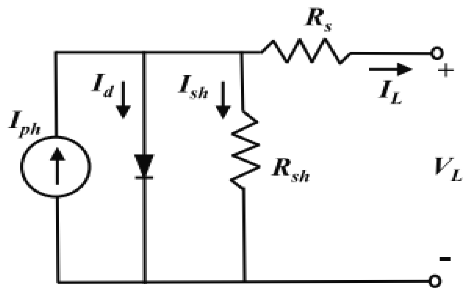
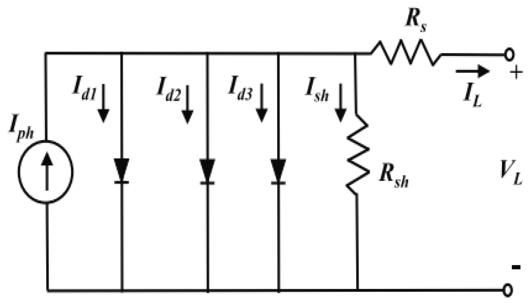
With the increasing severity of the global energy crisis as well as environmental pollution, it is particularly important to find sustainable energy solutions to replace traditional energy sources. Solar energy, as a pollution-free renewable form of energy, is becoming the focus of global attention [1,2]. Photovoltaic (PV) power generation systems are of vital importance for converting solar energy into electrical energy. To enhance the efficiency of power conversion in these systems, researchers have developed various PV models for simulation, control, and optimization purposes. These models include the single-diode model (SDM), double-diode model (DDM), three-diode model (TDM), and photovoltaic module model (MM), among others [3,4,5]. The accuracy of their parameters largely determines their performance. Regardless of the model employed, it is imperative to precisely ascertain these unknown parameters and ensure that the measurement data closely match the simulation data as much as possible [1,6]. Reliable models are essential to improve energy efficiency, strengthen energy management strategies, and optimize energy distribution in the grid [7].

At present, there are two main types of methods for parameter estimation in solar photovoltaic models, which are analytical methods and meta-heuristics. Analytical methods are methods for parameter estimation based on physical models and mathematical equations, for example, the direct extraction method, iterative method [8], simplified form method, Lambert-W based method [9], etc. The advantage of analytical methods is that their results are highly interpretable and have advantages in terms of theoretical foundation and flexibility, but they are particularly dependent on the prediction of the initial values, and if the initial parameters are not properly selected, they will fall into local optimization. In addition, such methods require long computational time and high computational power for parameter identification in PV models. In recent years, hybrid gray-box models and physics-informed heuristic methods have demonstrated significant potential in solar photovoltaic parameter estimation. Hybrid gray-box models effectively enhance prediction accuracy and generalization ability by combining data-driven algorithms (such as XGBoost, LSTM, and WaveNet) with physical mechanisms (such as solar radiation models and component efficiency curves). For instance, the research team at Beitai Tianyuan proposed a fusion architecture of XGBoost + LSTM + WaveNet, achieving a breakthrough in photovoltaic power prediction by reducing RMSE by 17∼34% through multi-scale feature fusion [10]. Such models not only capture the nonlinear relationships in historical data but also enhance the prediction stability under extreme weather conditions through physical constraints. The physical information heuristic method further integrates physical laws into the optimization algorithm. For instance, a hybrid model based on particle swarm optimization (PSO) and genetic algorithm (GA) quantifies the quantitative relationship between physical parameters such as solar radiation and temperature and power generation, significantly reducing prediction errors [11]. Additionally, the application of physical information neural networks (PINNs) in photovoltaic modeling has also attracted much attention. By adding a physical error penalty term to the loss function, it achieves joint training of data-driven and physical mechanisms, enhancing the model’s robustness in scenarios with scarce data [12]. Meta-heuristics constitute a category of optimization-based techniques aimed at extracting parameters. Optimization algorithms aim to reduce the discrepancy between the output of a model and corresponding actual measured data by exploring the parameter space. Widely used optimization algorithms encompass the genetic algorithm (GA), particle swarm optimization (PSO), differential evolutionary algorithm (DE), and the teaching–learning optimization algorithm (TLBO). These methods usually have global search capability and can avoid falling into local optimal solutions [8,9]. On the other hand, meta-heuristics are not limited by the complexity of the environment and the nonlinearity of the problem. In conclusion, meta-heuristic algorithms offer wide applicability, global search capability, and greater robustness compared to analytical methods when estimating PV model parameters. In the face of complex nonlinear models and noise interference, the meta-heuristic algorithm provides more accurate and reliable results for estimating parameters.

Taking into account the widespread popularity of the DE and PSO algorithms as fundamental approaches and the more frequent application of their variants compared to other algorithms in estimating solar PV model parameters, the following four primary categories of meta-heuristic algorithms stand out as the preferred choices for addressing the challenge of PV model parameter estimation: variants of DE, variants of PSO, hybrids of algorithms, and others. The first category is the variants of DE. Gao et al. comprehensively leveraged the data of the population along with the information derived from the directional vectors of differences to strengthen the global search proficiency of DE, and they suggested a permutation-based directional evolutionary algorithm with differential capabilities (DPDE) to tackle the estimation of parameters pertaining to diverse solar PV models [13]. Xiong et al. divided the population dynamics into three sub-populations and adopted different mutation strategies to enhance the ability of the algorithm to escape from local optima and improve the accuracy of parameter estimation (PSMDE) [14]. Kashif and colleagues developed a modification of DE by incorporating a penalty function. This enhancement led to the creation of a penalty-based differential evolutionary algorithm (P-DE) specifically designed for parameter extraction from solar PV modules across varying environmental conditions [15]. Biswas estimated the parameters for solar cells by using data sheet information under an adaptive differential evolution algorithm. The second category is the variants of PSO. Qaraad et al. introduced a dynamic optimization strategy and proposed a new PSO-based local search technique (QPSOL) to break through the limitations of PSO in the parameters determination for a PV model [16]. Lu et al. devised a multi-group collaborative search mechanism introduced into PSO and proposed a hybrid multi-swarm stochastic collaborative PSO (HMSCPSO) for parameter optimization of the models in PV system [17]. The third category is a hybrid of algorithms. Driss et al. combined the backtracking search optimization algorithm (BSA) with the DE to give full play to the advantages of BSA and DE to improve the parameter extraction accuracy of various photovoltaic models (DE/BSA) [18]. Li and colleagues introduced a combined adaptive teaching optimization algorithm based on DE (ATLDE) by mixing DE and TLBO and incorporating the learner’s ranking probabilities to derive diverse PV model parameters. Taleshian et al. integrated a technique known as the flexible improved PSO (FIPSO) with a gradient-guided sequential quadratic programming (SQP) approach for a comprehensive global search of PV parameters [19]. The last category contains a wide variety of algorithms, such as TLBO [20], the gray wolf optimization algorithm (GWO) [21], etc. Wang et al. proposed a rank-teaching–learning optimization algorithm based on reinforcement learning for PV model parameter estimation (RLRTLBO) [22]. However, these algorithms ignore the large differences in the feasible domains of the decision variables for the parameter estimation problem, which may affect the search efficiency. Because the feasible regions of the decision variables are quite different, using the same reproduction operator for them may lead to the omission of some optimal solution. With this in mind, we attempt to seek a new evolutionary algorithm or strategy in order to better solve this problem.

Although the above algorithms have achieved remarkable results on the parameter estimation problem of solar photovoltaic models, the design and improvement of these algorithms mainly focus on search performance and convergence speed. If the actual characteristics of the parameter estimation problem of the solar photovoltaic model are considered to design and improve the algorithm, whether the performance of the algorithm will be more improved. Gray predictive evolution algorithm (GPE) [23], which takes the gray model (GM(1,1)) as its theoretical basis, was firstly proposed by Hu et al. in 2020. Straightforward coding, limited controlling factors, robust search capabilities, and excellent robustness are the distinguishing features of GPE. These remarkable features of GPE make it frequently better than DE and PSO when dealing with complex optimization problems [24,25]. GPE selects different reproduction operators for each dimension of the individual vector for the reproduction process based on a threshold. Therefore, this paper chooses GPE as a basis optimizer to improve the precision as well as the robustness for solving solar parameter estimation problem by its unique search method.

The current improvement algorithms for GPE can be divided into the following two categories: The first category is based on the improvement of the algorithmic flow and operators. Dai et al. introduced a GPE utilized topological pairwise learning, referred to as TOGPEAe [24]. A novel fusion of GA and GPE approaches that determines the optimal scheduling for power generating units was proposed by Tong et al. [26]. A simplified non-isometric GPE was given by Xiang et al. [27]. Gao et al. developed a novel evolutionary algorithm for gray prediction by utilizing an enhanced gray model that incorporates a first-order inverse cumulative generation operation [28]. The second category is based on the improvement of the algorithmic control parameters. Gao et al. adaptively changed the control parameters of GPE and proposed four GPEs with different parameter settings, namely, GPE based on uniform distribution (aGPEu), GPE based on normal distribution (aGPEn), GPE based on average fitness (aGPEa), and GPE based on chaotic sequence-based GPE (aGPEc) [29].

Although these improved GPEs have worked well in many domains, researchers do not pay enough attention to GPE parameters, except Gao, who has studied its parameters. The control parameters of GPE determine its performance to a large extent, especially the threshold which controls the selection of propagating operators when GPE searches in each dimension. Meanwhile, the range gap of the PV model parameter estimation of current and voltage is too large, thus setting $\delta$ to 0.01–0.1 could lead to the selection of the same reproduction operator by most or even all individuals to the extent that the algorithm becomes trapped in a local optimum. Just imagine, if the threshold can be adaptively adjusted according to the value range of the decision variable, and the reproduction process can select the appropriate reproduction operators for each dimension of the individual variable, the search speed performance of the algorithm for solving the parameter estimation problem of the PV model may be improved.

Considering the practical significance of each decision variable in the solar energy parameter estimation problem and the great difference in the lengths of the value ranges, this paper proposes a gray predictive evolutionary algorithm with an adaptive threshold adjustment strategy (GPEat) to accurately identify PV parameters. Unlike previous GPEs and their variants, GPEat could adaptively adjust its thresholds based on the value ranges of the decision variables. The adaptively varying thresholds help to enhance the effectiveness of GPEat’s search in each dimension to some extent, which in turn improves the accuracy of GPEat’s prediction of PV model parameters. The performance of GPEat is verified through experimental comparison with eleven algorithms on five PV models.

The main work in this paper is shown as follows.

• Insight into the fact that disparities in domain lengths in different dimensions of the solar parameter estimation problem may affect the optimal performance of the algorithm.
• The gray predictive evolution algorithm (GPE) is firstly introduced in dealing with the parameter estimation problem of solar photovoltaic modeling.
• A gray predictive evolutionary algorithm with an adaptive threshold adjustment strategy (GPEat) is firstly proposed in this paper to solve the parameter estimation problem of solar photovoltaic modeling. Furthermore, an adaptive threshold adjustment strategy is designed in this algorithm to enhance the algorithm’s ability to automatically adjust and adapt to changes in the length of the problem domain.

ARTICLE FOLLOW-UP ARRANGEMENT: Section 2 introduces the mathematical modeling of the PV model. Section 3 illustrates the GPE as well as the threshold. Section 4 describes GPEat in detail. Section 4 elaborates the experimental results and analysis. Section 5 presents the conclusion and prospect of the whole paper.

2. Preliminaries

2.1. Mathematical Models of Photovoltaic Models

Mathematical models of photovoltaic (PV) cells are essential for understanding their nonlinear output behavior. Among the most commonly used PV models are the Single-Diode Model (SDM), Double-Diode Model (DDM), Triple-Diode Model (TDM), and PV Module Model (MM). The four models are described in detail below.

2.1.1. Single-Diode Model

The Single-Diode Model (SDM) describes the current-voltage (I-V) characteristics of a PV cell by modeling it as a diode. In SDM, the total current generated by the PV cell consists of three components, namely, the diode current ($I_d$), the photogenerated current ($I_{ph}$), and the current on the shunt resistor ($I_{sh}$). The diagram of the SDM is illustrated in Figure 1, where $I_{sd}$, $V_L$, $R_s$, and $R_{sh}$ represent the reverse saturation current of the diode, the output voltage, and the series and shunt resistances, respectively. By adjusting these model parameters, it is possible to fit the data of a real PV cell. The output current $I_L$ can then be formulated as follows.

$$\begin{array}{cc}\hfill I_L& =I_{ph}-I_d-I_{sh}\hfill \\ \hfill & =I_{ph}-I_{sd}[exp({\displaystyle \frac{q(V_L+R_s{I}_L)}{nkT}})-1]\hfill \\ & -{\displaystyle \frac{V_L+R_s{I}_L}{R_{sh}}}\hfill \end{array}$$

(1)

where the ideality factor of the diode is given by n, $q=1.60217646\times {10}^{-19}C$ denotes the charge of an electron, $k=1.3806503\times {10}^{-23}J/K$ is the Boltzmann constant, and T represents the cell temperature in Kelvin (°K). According to Equation (1), five parameters ($I_{ph},I_{sd},R_s,R_{sh}$, and n) are identified as unknown and must be accurately determined in SDM.

2.1.2. Double-Diode Model

The Double-Diode Model (DDM) accounts for the effects of both series and parallel resistances within a PV cell and describes its I-V characteristics more accurately than SDM. In DDM, the PV cell consists of an ideal diode and a non-ideal diode in series. The corresponding mathematical formula and structural diagram are shown in Equation (2) and Figure 2, respectively. By adjusting the model parameters, the data from an actual PV cell can be more accurately fitted.

$$\begin{array}{cc}\hfill I_L& =I_{ph}-I_{d_1}-I_{d_2}-I_{sh}\hfill \\ \hfill & =I_{ph}-I_{s{d}_1}[exp({\displaystyle \frac{q(V_L+R_s{I}_L)}{n_{1}kT}})-1]\hfill \\ & -I_{s{d}_2}[exp({\displaystyle \frac{q(V_L+R_s{I}_L)}{n_{2}kT}})-1]\hfill \\ & -{\displaystyle \frac{V_L+R_s{I}_L}{R_{sh}}}\hfill \end{array}$$

(2)

in which the diffusion and saturation currents are represented by $I_{d_1}$ and $I_{d_2}$, respectively, while the ideality factors of the two diodes are denoted by $n_1$ and $n_2$. The parameters $I_{ph}$, $I_{s{d}_1}$, $I_{s{d}_2}$, $R_s$, $R_{sh}$, $n_1$ and $n_2$ in Equation (2) are unknown and need to be determined.

2.1.3. Triple-Diode Model

Compared to the DDM, the Triple-Diode Model (TDM) is more complex and powerful for using three diodes. The TDM is suitable for intricate circuit applications but requires a longer execution time. The structure of the TDM is shown in Figure 3, and the corresponding mathematical formula is given in the following equation.

$$\begin{array}{cc}\hfill I_L& =I_{ph}-I_{d_1}-I_{d_2}-I_{d_3}-I_{sh}\hfill \\ \hfill & =I_{ph}-I_{s{d}_1}[exp({\displaystyle \frac{q(V_L+R_s{I}_L)}{n_{1}kT}})-1]\hfill \\ & -I_{s{d}_2}[exp({\displaystyle \frac{q(V_L+R_s{I}_L)}{n_{2}kT}})-1]\hfill \\ & -I_{s{d}_3}[exp({\displaystyle \frac{q(V_L+R_s{I}_L)}{n_{3}kT}})-1]-{\displaystyle \frac{V_L+R_s{I}_L}{R_{sh}}}\hfill \end{array}$$

(3)

where $I_{s{d}_3}$ and $n_3$ represent the saturation current and ideality factor of the third diode, respectively. $I_{ph}$, $I_{s{d}_1}$, $I_{s{d}_2}$, $I_{s{d}_3}$, $R_s$, $R_{sh}$, $n_1$, $n_2$, and $n_3$ in Equation (3) are nine unknown parameters to be identified.

2.1.4. PV Module Model

The PV Module Model (MM) represents a solar cell module, which is a general term for a set of solar cells connected in series or parallel configurations. The MM is commonly used in solar power generation systems to produce electricity. As shown in Figure 4, the MM comes in different specifications and capacities, depending on the application scenario. The equation provided below is used to determine the output current of the MM.

$$\begin{array}{cc}\hfill I_L& =I_{ph}{N}_p-I_{sd}{N}_p[exp({\displaystyle \frac{q(V_L{N}_p+R_s{I}_L{N}_s)}{nkT{N}_s{N}_p}})-1]\hfill \\ \hfill & -{\displaystyle \frac{V_L{N}_p+R_s{I}_L{N}_s}{R_{sh}{N}_s}}\hfill \end{array}$$

(4)

in which the number of solar cells connected in parallel and series are represented by $N_p$ and $N_s$, respectively. As shown in Equation (4), MM similarly to SDM involves five unknown parameters.

2.1.5. Objective Function

Like most optimization problems, the identification of the parameters of PV models is a problem for finding an optimal solution. In the problem, the objective is to identify a set of parameters that minimizes the discrepancy between the simulated and experimentally measured current data. The root mean square error (RMSE) is a commonly used metric for assessing error and is frequently referenced in various academic works [15,30,31]. The RMSE serves as an objective criterion to evaluate the accuracy of the predictive outcomes generated by a forecasting model. The expression for the RMSE is as follows.

$$RMSE=\sqrt{{\displaystyle \frac{{\sum }_{i=1}^{N}f{(V_L,I_L,X)}^2}{N}}}$$

(5)

where N represents the number of experimental data, X denotes the vector of unknown parameters, and f represents the error function.

For the SDM, X and f are defined, respectively, as Equation (6).

$$\left\{\begin{array}{cc}\hfill X& =[I_{ph},I_{sd},R_s,R_{sh},n]\hfill \\ \hfill f(V_L,I_L,X)& =I_{ph}-I_L-I_{sd}[exp({\displaystyle \frac{q(V_L+R_s{I}_L)}{nkT}})-1]\hfill \\ \hfill & -{\displaystyle \frac{V_L+R_s{I}_L}{R_{sh}}}\hfill \end{array}\right.$$

(6)

For the DDM, X and f are defined, respectively, as Equation (7).

$$\left\{\begin{array}{cc}\hfill X& =[I_{ph},I_{s{d}_1},I_{s{d}_2},R_s,R_{sh},n_1,n_2]\hfill \\ \hfill f(V_L,I_L,X)& =I_{ph}-I_L-I_{s{d}_1}[exp({\displaystyle \frac{q(V_L+R_s{I}_L)}{n_{1}kT}})-1]\hfill \\ \hfill & -I_{s{d}_2}[exp({\displaystyle \frac{q(V_L+R_s{I}_L)}{n_{2}kT}})-1]-{\displaystyle \frac{V_L+R_s{I}_L}{R_{sh}}}\hfill \end{array}\right.$$

(7)

For the TDM, X and f are defined, respectively, as Equation (8).

$$\left\{\begin{array}{cc}\hfill X& =[I_{ph},I_{s{d}_1},I_{s{d}_2},I_{s{d}_3},R_s,R_{sh},n_1,n_2,n_3]\hfill \\ \hfill f(V_L,I_L,X)& =I_{ph}-I_L-I_{s{d}_1}[exp({\displaystyle \frac{q(V_L+R_s{I}_L)}{n_{1}kT}})-1]\hfill \\ \hfill & -I_{s{d}_2}[exp({\displaystyle \frac{q(V_L+R_s{I}_L)}{n_{2}kT}})-1]\hfill \\ \hfill & -I_{s{d}_3}[exp({\displaystyle \frac{q(V_L+R_s{I}_L)}{n_{3}kT}})-1]-{\displaystyle \frac{V_L+R_s{I}_L}{R_{sh}}}\hfill \end{array}\right.$$

(8)

For the MM, X and f are defined, respectively, as Equation (9).

$$\left\{\begin{array}{cc}\hfill X& =[I_{ph},I_{sd},R_s,R_{sh},n]\hfill \\ \hfill f(V_L,I_L,X)& =I_{ph}{N}_p-I_L\hfill \\ \hfill & -I_{sd}{N}_p[exp({\displaystyle \frac{q(V_L{N}_p+R_s{I}_L{N}_s)}{nkT{N}_s{N}_p}})-1]\hfill \\ \hfill & -{\displaystyle \frac{V_L{N}_p+R_s{I}_L{N}_s}{R_{sh}{N}_s}}\hfill \end{array}\right.$$

(9)

2.2. Gray Prediction Evolutionary Algorithm

The gray prediction evolutionary algorithm (GPE) was first proposed by Hu et al. in 2020 [23] as a heuristic global optimization method based on gray prediction theory. In GPE, population evolution is treated as a time series where an even gray model (EGM(1,1)) serves as the reproduction operator to predict the solutions in the subsequent generation. The algorithmic framework of GPE is outlined as follows.

2.2.1. Initialization

GPE begins by initializing three generation populations ($X^0$, $X^1$, and $X^2$), each of which comprises N D-dimensional individuals within the search space. The i-th individual in the t-th generation is denoted as ${\overrightarrow{x}}_i^t=(x_{i,1}^t,x_{i,2}^t,\cdots ,x_{i,D}^t),i=1,2,\dots ,N,t=0,1,2,\dots ,t_{max}$, where $t_{max}$ represents the maximum number of iterations. In the initialization operator, a random uniform distribution is employed to generate the j-th ($j=1,2,\dots ,D$) dimension of the i-th individual as follows.

$$x_{i,j}^t=L_j+rand(0,1)·(U_j-L_j)$$

(10)

where $rand(0,1)$ represents a random number uniformly distributed within $[0,1]$, $U_j$ is the upper limit for the j-th dimension, and $L_j$ is the corresponding lower limit.

According to Equation (10), $3N$ D-dimensional individuals are generated, sorted by their fitness values from worst to best, and then assigned to populations $X^0$, $X^1$, and $X^2$.

2.2.2. Reproduction Operator

Taking $X^t$ ($t⩾2$) as a target population, three consecutive populations, $X^{t-2}$, $X^{t-1}$, and $X^t$, are treated as a population series $\{X^{t-2},X^{t-1},X^t\}$. Subsequently, three individuals, ${\overrightarrow{x}}_{r_1}$, ${\overrightarrow{x}}_{r_2}$, and ${\overrightarrow{x}}_{r_3}$, are randomly selected from the population series $X^{t-2}$, $X^{t-1}$, $X^t$ in succession. Define $d_{12}=|x_{r_1,j}^{t-2}-x_{r_2,j}^{t-1}|$, $d_{13}=|x_{r_1,j}^{t-2}-x_{r_3,j}^t|$, and $d_{23}=|x_{r_2,j}^{t-1}-x_{r_3,j}^t|$. Let $Ma{x}_{d_r}=max\{d_{12},d_{13},d_{23}\}$ and $Mi{n}_{d_r}=min\{d_{12},d_{13},d_{23}\}$. The j-th element of a trial vector ${\overrightarrow{u}}_i^t=(u_{i,1}^t,u_{i,2}^t,\dots ,u_{i,j}^t,\dots ,u_{i,D}^t)$ is generated using the reproduction operator of GPE, which is given by Equation (11).

$$u_{i,j}^t=\left\{\begin{array}{c}(x_{r_1,j}-{\displaystyle \frac{\beta }{\alpha }})·(1-e^{\alpha })·e^{-3\alpha },\mathrm{if}Ma{x}_{d_r}\ge \delta ,\hfill \\ {\displaystyle \frac{4x_{r_3,j}+x_{r_2,j}-2x_{r_1,j}}{3}},\mathrm{elseif}Mi{n}_{d_r}<\delta ,\hfill \\ x_{r_3,j}+\omega ·Ma{x}_{d_r},\mathrm{otherwise}.\hfill \end{array}\right.$$

(11)

where $\delta$ is a threshold to control prediction, $\alpha$ is a gray developmental coefficient, $\beta$ is a gray control parameter, and $\omega$ is a disturbance coefficient. The formulas for $\alpha$, $\beta$, and $\omega$ are given as follows.

$$\begin{array}{cc}\hfill \alpha & ={\displaystyle \frac{2(x_{r_2,j}-x_{r_3,j})}{x_{r_2,j}+x_{r_3,j}}}\hfill \end{array}$$

(12)

$$\begin{array}{cc}\hfill \beta & ={\displaystyle \frac{2({(x_{r_2,j})}^2+x_{r_1,j}·x_{r_2,j}-x_{r_1,j}·x_{r_3,j})}{x_{r_2,j}+x_{r_3,j}}}\hfill \end{array}$$

(13)

$$\begin{array}{cc}\hfill \omega & =rand(-1,1)·(0.01-{\displaystyle \frac{(t-t_{max})}{t_{max}}})\hfill \end{array}$$

(14)

where $rand(-1,1)$ represents a random number within the range of $[-1,1]$, t denotes the current iteration, and $t_{max}$ is the maximum number of iterations.

2.2.3. Selection Operator

A greedy selection strategy is employed to ensure the survival of the most promising individuals across generations. Specifically, if the objective function value of a trial individual ${\overrightarrow{u}}_i^t$ is better than that of the target individual ${\overrightarrow{x}}_i^t$, the trial individual ${\overrightarrow{u}}_i^t$ is selected for the next generation. Otherwise, the target individual ${\overrightarrow{x}}_i^t$ is retained in the next generation population, denoted as $X^{t+1}=({\overrightarrow{x}}_1^{t+1},{\overrightarrow{x}}_2^{t+1},\dots ,{\overrightarrow{x}}_N^{t+1})$. The selection operator of GPE can be expressed in the following form.

$${\overrightarrow{x}}_i^{t+1}=\left\{\begin{array}{c}{\overrightarrow{u}}_i^t,\mathrm{if}fitness({\overrightarrow{u}}_i^t)<fitness({\overrightarrow{u}}_i^t)\hfill \\ {\overrightarrow{x}}_i^t,\mathrm{otherwise}.\hfill \end{array}\right.$$

(15)

2.3. Reproductive Process of Differential Evolution Algorithm

Meta-heuristics including differential evolution (DE) [32] and particle swarm optimization (PSO) [33] are commonly used for initialization in current improvement algorithms of GPE. Referring to the recent non-equidistant gray prediction evolutionary algorithm (NeGPE) [25], the reproduction process of DE is chosen to initialize the population of the first three generations in this paper. The reproduction process of DE includes mutation, crossover and selection, which are introduced as follows.

Mutation Mutation generates a new individual, known as the mutant vector, by adding the scaled difference between two randomly selected individuals to a third individual. This ensures diversity in the population, which aids in exploring the solution space. The mutation formula is defined as follows.

$${\overrightarrow{u}}_i={\overrightarrow{x}}_{r_1}+F·({\overrightarrow{x}}_{r_2}-{\overrightarrow{x}}_{r_3})$$

(16)

where ${\overrightarrow{x}}_{r_1},{\overrightarrow{x}}_{r_2},{\overrightarrow{x}}_{r_3}$ are distinct randomly selected individuals from the current population, and F is a mutation scaling factor, which controls the amplification of the difference vector.

Crossover After mutation, the crossover operation combines the mutant vector with the target vector to produce a trial vector. The goal of the crossover is to introduce new genetic material into the offspring. The crossover is applied component-wise with a crossover probability $CR$, which determines the likelihood that a gene from the mutant vector will replace the corresponding gene in the target vector. The trial vector ${\overrightarrow{v}}_i$ is generated as follows.

$$v_{i,j}=\left\{\begin{array}{cc}{u}_{i,j},\hfill & \mathrm{if}randb(j)\le CR\hfill \\ x_{i,j},\hfill & \mathrm{otherwise}\hfill \end{array}\right.$$

(17)

where $j=1,2,\dots ,D$,$randb(j)$ is a random number between 0 and 1, and $CR$ is the crossover probability, controlling the extent of gene exchange between the target and mutant vectors.

Selection The selection process determines which individuals will enter the next generation. The trial vector ${\overrightarrow{v}}_i$ and the target vector ${\overrightarrow{x}}_i$ are compared based on their fitness values. If the fitness of the trial vector is better, it replaces the target vector in the population; otherwise, the target vector is retained. The selection process can be formalized as follows.

$${\overrightarrow{x}}_i^{new}=\left\{\begin{array}{cc}{\overrightarrow{v}}_i,\hfill & \mathrm{if}f({\overrightarrow{v}}_i)<f({\overrightarrow{x}}_i)\hfill \\ {\overrightarrow{x}}_i,\hfill & \mathrm{otherwise}\hfill \end{array}\right.$$

(18)

where $f({\overrightarrow{v}}_i)$ and $f({\overrightarrow{x}}_i)$ are the fitness values of the trial and target vectors, respectively. This ensures that only the best solutions are retained for the next generation.

3. Proposed Algorithm

Previous improvements to Gray Prediction Evolutionary (GPE) algorithms primarily fall into two categories. The first focuses on enhancing algorithmic structures and operators, exemplified by approaches like TOGPEAe, which integrates topological pairwise learning, and hybrid GA-GPE frameworks for power scheduling optimization. The second category emphasizes adaptive control parameter tuning, as demonstrated in Gao et al.’s work—particularly their adaptive GPE variants (e.g., aGPEu, aGPEn), which dynamically adjust parameters such as distribution types or chaotic sequences to optimize search performance. This approach aligns with the parameter-adaptive philosophies underlying early DE/PSO variants, wherein parameters self-modify to enhance algorithmic exploration-exploitation balance. Building on these foundations, this study introduces an Adaptive Threshold Adjustment Strategy (ATS) for GPE, specifically tailored to address multi-scale decision variable ranges in solar energy parameter estimation. By dynamically calibrating operator selection thresholds based on variable value ranges, ATS enhances GPE’s adaptability and solution precision in complex optimization scenarios. In this section, the main framework of a gray predictive evolutionary algorithm with an adaptive threshold adjustment strategy (GPEat) is first proposed, followed by a detailed description of the adaptive threshold adjustment strategy (ATS). After that, the third subsection is the analysis and discussion of ATS based on GPEat.

3.1. The Framework of GPEat

Algorithm 1 presents the pseudo-code for implementing GPEat. The proposed GPEat algorithm initializes N individuals by using Latin Hypercube Sampling (LHS), thus generating the first population $X^0$ (line 1). Subsequently, the reproduction process of DE is applied to generate the second and third generations, $X^1$ and $X^2$, respectively, (line 2). The reproduction process is performed as Equation (16) to Equation (18). $X^2$ is considered as the parent population of the next generation of offspring. Next, the following procedure is repeated until the maximum number of FEs $Max\_FEs$ is reached. Based on the proposed adaptive threshold adjustment strategy (ATS), the appropriate reproduction operator is selected to generate the offspring, as detailed in Algorithm 2 (lines 7–8). After generating the offspring, the fitness values of the parent and the offspring are compared, and the individual with the better fitness value is selected as the population in the next generation (lines 9–12).

Algorithm 1: Framework of GPEat

Algorithm 2: Selection of reproduction operators based on ATS

3.2. Adaptive Threshold Adjustment Strategy

A suitable threshold is crucial for the optimization performance of the proposed algorithm. The choice of threshold determines the reproduction process of the algorithm. In this paper, an adaptive threshold adjustment strategy (ATS) is presented. The ATS strategy is used to generate suitable thresholds for different dimensions of an individual by adapting different feasible region ranges for different dimensions of an individual. Specifically, the threshold $\delta$ in ATS is defined by Equation (19).

$$\delta ={\displaystyle \frac{UB(j)-LB(j)}{N}},j=1,2,\cdots ,D$$

(19)

where D is the dimension of an individual. $UB$ and $LB$ denote the upper and lower bounds on the feasible region of the dimension of the individual, respectively. N is a positive integer.

For the parameter estimation problem of photovoltaic (PV) models, a sensitivity analysis was conducted on the parameter N by systematically varying its values within the set $N\in 1,2,\dots ,10,20,\dots ,100$ across five benchmark PV models. The experimental results revealed that N exhibits a sensitive range of [5, 10], within which the algorithm achieves a trade-off between solution accuracy and computational efficiency. Notably, $N=8$ was identified as the optimal default value, balancing precision and convergence speed effectively.

After obtaining the appropriate threshold $\delta$ according to Equation (19), the offspring ${\overrightarrow{u}}_i^t$ could be obtained by the reproduction process according to the following formula.

$$u_{i,j}^t=\left\{\begin{array}{c}(x_{r_1,j}-{\displaystyle \frac{\beta }{\alpha }})·(1-e^{\alpha })·e^{-3\alpha },\mathrm{if}Ma{x}_{d_r}\ge \delta ,\hfill \\ {\displaystyle \frac{4x_{r_3,j}+x_{r_2,j}-2x_{r_1,j}}{3}},\mathrm{otherwise}.\hfill \end{array}\right.$$

(20)

where $\alpha$ and $\beta$ are calculated according to Equation (12) and Equation (13), respectively.

It is worth noting that considering the instability of the random perturbation operator of the original GPE, the reproduction process of ATS-based GPEat is missing the random perturbation operator compared to the original GPE. Pseudo-code of the reproduction process of ATS-based GPEat is presented in Algorithm 2.

3.3. Analysis of Adaptive Threshold Adjustment Strategy

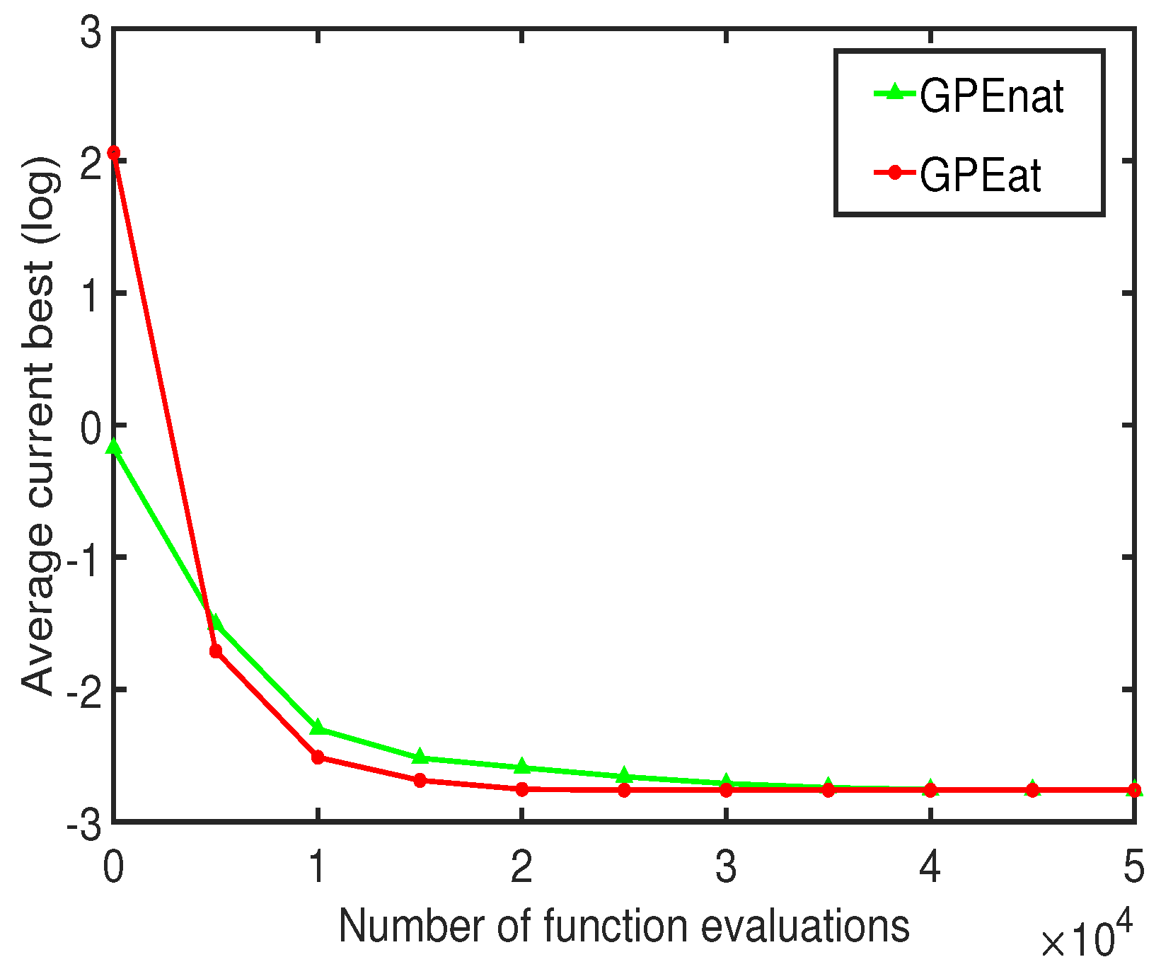
The existing adaptive techniques in DE and PSO usually focus on dynamically adjusting control parameters or weights according to the search performance of algorithms, such as JADE [34], SaDE [35] and APSO [36]. In contrast, the ATS in GPEat is specifically designed for the threshold parameters used in the reproduction operator, which is crucial for selecting appropriate mutation strategies for different dimensions of the solution space. This targeted adjustment enables GPEat to better handle the significant differences in the feasible regions of decision variables inherent in the problem of parameter estimation for photovoltaic models. In the GPEat algorithm, ATS is designed to use the threshold proportional to the range of each dimension variable of a individual vector to select an appropriate replication operator to generate the next generation of the individual. In order to verify the effectiveness of ATS in GPEat, an ablation experiment concerning ATS with and without ATS within the same algorithmic framework of GPEat is performed. The algorithm without ATS under the same algorithmic framework of GPEat is denoted as GPEnat. GPEat and GPEnat are tested on the STM640/36 model to evaluate the impact of ATS on the performance of the algorithm for the PV problem. The maximum number of function evaluations (FEs) is set to 5000. The convergence curve of one random run is shown in Figure 5, while the usage of the gray prediction operator is shown in Figure 6.

As shown in Figure 5 and Figure 6, whether ATS is adopted within the same algorithm framework or not leads to significant differences in the search performance of the algorithm and the use of the gray prediction operator. In Figure 5, careful observation reveals that GPEat has converged around $FEs=$ 20,000, while GPEnat is still searching optimal solution. It can be clearly seen from Figure 6 that the utilization of the gray prediction operator in GPEat is more frequent for the $I_{sd}$ parameter compared to GPEnat, whereas its usage is relatively infrequent for the parameters $I_{ph},R_s,R_{sh}$, and n. The domain lengths of $I_{ph},I_{sd},R_s,R_{sh}$, and n are 2, 5 × 10⁻⁵, 0.36, 1000, and 59, respectively, leading to disparities in the frequency of the gray prediction operator’s application. This is bound to cause the algorithm to fall into local optimum. Notably, during the optimization process of GPEnat, the $I_{sd}$ parameter does not utilize the gray prediction operator at all, possibly due to its domain length or other factors.

Obviously, the proposed ATS effectively adjusts the proportion of the two types of reproduction operators within the population, overcoming the issue of confining all individuals to a single reproduction operator. This strategy achieves a balance between convergence speed and stability, thereby enabling GPEat suitable for the PV problem.

3.4. Theoretical Analysis of Algorithm Characteristics: Convergence and Complexity

In the field of algorithm design, convergence is a crucial metric for evaluating whether an algorithm can ultimately find the optimal or near-optimal solution. For the Gray Predictive Evolutionary Algorithm with an Adaptive Threshold Adjustment Strategy (GPEat) proposed in this paper, we analyze its convergence using the knowledge of Markov chains in stochastic process theory.

The search process of the GPEat algorithm can be abstracted as a Markov process. In this process, A continuous three-generation populations are defined as a state, and state transitions are determined by the reproduction operators (such as crossover and mutation) used by the algorithm and the Adaptive Threshold Adjustment Strategy (ATS).

The ATS is one of the core innovations of the GPEat algorithm. It adjusts the threshold proportionally according to the length of each decision variable. This dynamic adjustment mechanism endows the algorithm with the ability to flexibly select appropriate reproduction operators in search spaces of different dimensions. Theoretically, this flexibility helps the algorithm avoid getting trapped in local optimal solutions.

Assume that the search space is finite and discrete, and the reproduction operators of the algorithm satisfy certain probability distribution conditions. According to the convergence theorem of Markov chains, if the state-transition matrix of a Markov chain is ergodic, then the Markov chain will converge to a steady-state distribution. In the GPEat algorithm, due to the existence of the ATS, the algorithm can adaptively adjust the search direction and step-size at different search stages. This enables the algorithm to have the opportunity to visit all possible states in the search space during the search process, thus ensuring the ergodicity of the state-transition matrix. Therefore, we can infer that the GPEat algorithm has the property of converging to the global optimal solution in theory.

4. Experimental Results

The superior performance of GPEat is analyzed below by contrasting the parameter identification across various PV models of them to that of other algorithms. For the SDM and DDM, the I-V data were acquired from a commercially available R.T.C. French solar cells, measuring 57 mm in diameter, at a consistent temperature of 33 °C [37,38]. Additionally, the study evaluates single-crystal STM6 40/36 and polycrystalline STP6-120/36, as well as Photowatt-PWP201 panels, with I-V data referenced from [39,40,41].

Table 1. Parameter range for the single- and double-diode models and the PV module model.

Parameters	R.T.C. France Solar Cell		STM6-40/36		STP6-120/36		Photowatt-PWP-201
	LB	UB	LB	UB	LB	UB	LB	UB
$I_{ph}$(A)	0	1	0	2	0	8	0	2
$I_{sd},I_{s{d}_1},I_{s{d}_2},I_{s{d}_3}$($\mu A$)	0	1	0	50	0	50	0	50
$n_1,n_2,n_3$	1	2	1	60	1	50	1	50
$R_{sh}$($\mathrm{\Omega }$)	0	100	0	1000	0	1500	0	2000
$R_s$($\mathrm{\Omega }$)	0	0.5	0	0.36	0	0.36	0	2

specifies the parameter bounds for all models discussed, with LB and UB indicating the lower and upper limits, respectively. Note that many researchers have adopted such a parameter search range. The comparison algorithms include four popular DE variants DPDE [13], JDE [42], PSMDE [14] and HDE [43], three variants of the recently popular teaching optimization algorithm ATLDE [44], RLRTLBO [22] and MTLBO [45], and the advanced algorithms LSHADE [46], DE/BSA [18], IJAYA [47], and CLPSO [48], which are designed for PV model parameter extraction. Each model’s MaxFEs are capped at 50,000.

Table 2. Parameter settings of compared algorithms.

Algorithms	Parameter Settings
GPEat	$NP=40,F=0.7,CR=0.7,Maxgen=1500,N=8$
ATLDE	$NP=50,F=0.5$
PSMDE	$NP=40$
RLRTLBO	$NP=20$
DE/BSA	c$NP=30,F\in [0.1,0.9],Cr\in [0.1,0.9]$
HDE	$NP=30,p=0.1$
DPDE	$N{P}^{init}=18\times D,p=0.11,H=5$
CLPSO	$NP=40,w=0.9\sim 0.2,c=1.496,m=5$
MTLBO	$NP=50$
LSHADE	$NP=20,\epsilon$ = 0.05 or 0.01 or 1.5
JDE	c$NP=30,F=0.5,CR=0.9$
IJAYA	c$NP=20$

details the configurations for each algorithm and summarizes the outcomes from 30 independent trials per method. The implementations of GPEat and ATLDE were executed using Matlab 2022b on a desktop equipped by an Intel Core i7-7500U CPU at 3.50 GHz, 4 GB RAM, running on Windows 10 64-bit OS. Out of respect for the original research, data from comparative algorithms are directly cited from their respective publications.

4.1. Results on the SDM

The statistical results of the Root Mean Square Error (RMSE) values derived from all the algorithms applied to the SDM of the R.T.C. France solar cell is presented in

Table 3. Statistical results of the RMSE values obtained by compared algorithms for the single-diode model.

Algorithms	RMSE
	Max	Min	Mean	Std
GPEat	9.8602187789 $\times {10}^{-4}$	9.8602187789 $\times {10}^{-4}$	9.8602187789 $\times {10}^{-4}$	2.0033222035 $\times {10}^{-17}$
ATLDE	9.8602187789 $\times {10}^{-4}$	9.8602187789 $\times {10}^{-4}$	9.8602187789 $\times {10}^{-4}$	2.2081921801 $\times {10}^{-17}$
PSMDE	9.8602187789 $\times {10}^{-4}$	9.8602187789 $\times {10}^{-4}$	9.8602187789 $\times {10}^{-4}$	2.0821123455 $\times {10}^{-17}$
RLRTLBO	9.8602187789 $\times {10}^{-4}$	9.8602187789 $\times {10}^{-4}$	9.8602187789 $\times {10}^{-4}$	1.87 $\times {10}^{-17}$
DE/BSA	9.8602187789 $\times {10}^{-4}$	9.8602187789 $\times {10}^{-4}$	9.8602187789 $\times {10}^{-4}$	2.4315408969 $\times {10}^{-17}$
HDE	9.8602187789 $\times {10}^{-4}$	9.8602187789 $\times {10}^{-4}$	9.8602187789 $\times {10}^{-4}$	4.5699449531 $\times {10}^{-17}$
DPDE	9.8602187789 $\times {10}^{-4}$	9.8602187789 $\times {10}^{-4}$	9.8602187789 $\times {10}^{-4}$	2.5711448159 $\times {10}^{-17}$
CLPSO	2.2761949373 $\times {10}^{-3}$	9.8603019909 $\times {10}^{-4}$	1.5132594325 $\times {10}^{-3}$	4.5462781638 $\times {10}^{-4}$
MTLBO	9.8602187789 $\times {10}^{-4}$	9.8602187789 $\times {10}^{-4}$	9.8602187789 $\times {10}^{-4}$	1.9092749355 $\times {10}^{-17}$
LSHADE	9.8602187789 $\times {10}^{-4}$	9.8602187789 $\times {10}^{-4}$	9.8602187789 $\times {10}^{-4}$	2.7247138599 $\times {10}^{-17}$
JDE	9.8602187789 $\times {10}^{-4}$	9.8602187789 $\times {10}^{-4}$	9.8602187789 $\times {10}^{-4}$	2.4775498278 $\times {10}^{-17}$
IJAYA	9.9478795708 $\times {10}^{-4}$	9.8617061742 $\times {10}^{-4}$	9.8904639903 $\times {10}^{-4}$	2.2987962420 $\times {10}^{-6}$

. This table illustrates the range of results by detailing the minimum (Min), maximum (Max), average (Mean), and standard deviation (Std) of the RMSE values.

It is evident from Table 3 that GPEat, ATLDE, PSMDE, RLRTLBO, DE/BSA, HDE, DPDE, MTLBO, LSHADE, and JDE obtain optimal values for the Min, Max, and Mean that demonstrate the relatively high accuracy of solutions provided by these seven algorithms, succeeded by IJAYA and CLPSO. As far as the stability of all comparative algorithms, GPEat shows the best performance. It indicates that the robustness of the proposed algorithm is significantly better than other compared algorithms on this experiment.

The optimal RMSE along with the respective identified parameter values are given in

Table 4. Performance comparison between NeGPEat and its competitors regarding the best estimated parameters on the SDM.

Algorithms	${\mathit{I}}_{\mathit{ph}}$ (A)	${\mathit{I}}_{\mathit{sd}}$ ($\mathit{\mu }\mathit{A}$)	${\mathit{R}}_{\mathit{s}}$ ($\mathbf{\Omega }$)	${\mathit{R}}_{\mathit{sh}}$ ($\mathbf{\Omega }$)	a	RMSE
GPEat	0.76078	0.32302081	0.03637709	53.718525	1.48118359	9.8602187789 $\times {10}^{-4}$
ATLDE	0.76078	0.32302080	0.03637709	53.718524	1.48118359	9.8602187789 $\times {10}^{-4}$
PSMDE	0.76078	0.32302083	0.03637709	53.718526	1.48118359	9.8602187789 $\times {10}^{-4}$
RLRTLBO	0.7608	0.3230	0.0364	53.7185	1.4812	9.86022 $\times {10}^{-4}$
DE/BSA	0.76078	0.32302080	0.0363770	53.7185246	1.48118359	9.8602187789 $\times {10}^{-4}$
HDE	0.76078	0.32302082	0.03637709	53.718525	1.48118359	9.8602187789 $\times {10}^{-4}$
DPDE	0.76078	0.32302079	0.03637709	53.718523	1.48118358	9.8602187789 $\times {10}^{-4}$
CLPSO	0.76078	0.32233513	0.03638559	53.660233	1.48096971	9.8603019909 $\times {10}^{-4}$
MTLBO	0.76078	0.32302082	0.03637709	53.718524	1.48118359	9.8602187789 $\times {10}^{-4}$
LSHADE	0.76078	0.32302082	0.03637709	53.718525	1.84118359	9.8602187789 $\times {10}^{-4}$
JDE	0.76078	0.32302082	0.03637709	53.718525	1.48118359	9.8602187789 $\times {10}^{-4}$
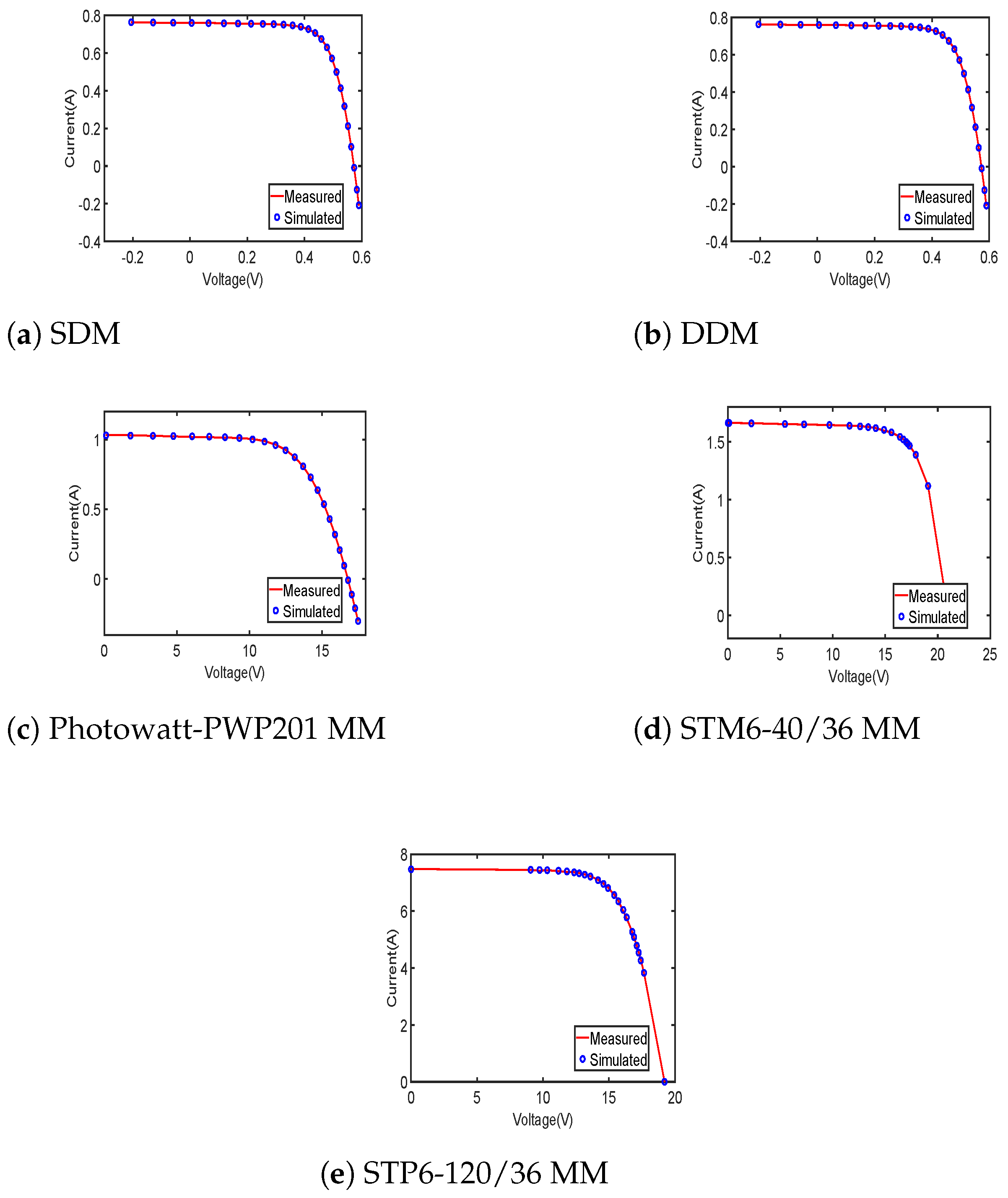
IJAYA	0.76078	0.32302083	0.03637709	53.778526	1.48118360	9.8617061742 $\times {10}^{-4}$

. It is evident that GPEat, ATLDE, HDE, DPDE, MTLBO, LSHADE, and JDE have obtained the best RMSE and the associated values of recognition parameters, CLPSO and IJAYA, also yield almost optimal values. Furthermore, the simulated I-V curves shown in Figure 7a are employed to exhibit the degree of conformity between the simulated and experimental data to demonstrate the precision of the identification parameter values derived from GPEat. Furthermore, it can be seen from Figure 7a that there have minimal discrepancies between them.

Figure 8 offers graphical representations of the convergence processes for six out of the total comparative algorithms, from which it can be seen that MTLBO converges the fastest, followed by GPEat and ATLDE. The three algorithms reach the optimal solution at FEs = 5000; meanwhile, the other algorithms are still in the process of seeking the optimal solution, indicating that GPEat exhibits quicker global convergence.

4.2. Results on the DDM

As outlined in Section 2, identifying seven parameters is necessary for the DDM. The statistical results of the different algorithms are shown in

Table 5. Statistical results of the RMSE values obtained by compared algorithms for the double-diode model.

Algorithms	RMSE
	Max	Min	Mean	Std
GPEat	9.8602187789 $\times {10}^{-4}$	9.8248485179 $\times {10}^{-4}$	9.8320172957 $\times {10}^{-4}$	1.2729158018 $\times {10}^{-6}$
ATLDE	9.9878961732 $\times {10}^{-4}$	9.8259906028 $\times {10}^{-4}$	9.8576807726 $\times {10}^{-4}$	2.6353200897 $\times {10}^{-6}$
PSMDE	9.8602418768 $\times {10}^{-4}$	9.8248485179 $\times {10}^{-4}$	9.8271897710 $\times {10}^{-4}$	7.5940250210 $\times {10}^{-7}$
RLRTLBO	9.8602187789 $\times {10}^{-4}$	9.8248485179 $\times {10}^{-4}$	9.8378189238 $\times {10}^{-4}$	1.73 $\times {10}^{-6}$
DE/BSA	9.8672330355 $\times {10}^{-4}$	9.8248485178 $\times {10}^{-4}$	9.8386784427 $\times {10}^{-4}$	1.5678462931 $\times {10}^{-6}$
HDE	9.8602187789 $\times {10}^{-4}$	9.8248485179 $\times {10}^{-4}$	9.8415447876 $\times {10}^{-4}$	1.6726437317 $\times {10}^{-6}$
DPDE	9.8308142049 $\times {10}^{-4}$	9.8248482716 $\times {10}^{-4}$	9.8254977938 $\times {10}^{-4}$	1.5133379716 $\times {10}^{-7}$
CLPSO	1.8710162060 $\times {10}^{-3}$	9.8684968998 $\times {10}^{-4}$	1.3755723403 $\times {10}^{-3}$	2.7152516507 $\times {10}^{-4}$
MTLBO	1.5767485449 $\times {10}^{-3}$	9.8248487604 $\times {10}^{-4}$	1.1564617247 $\times {10}^{-3}$	1.4395895110 $\times {10}^{-4}$
LSHADE	1.6245206409 $\times {10}^{-3}$	9.8248485179 $\times {10}^{-4}$	1.0041527554 $\times {10}^{-3}$	1.1717097265 $\times {10}^{-4}$
JDE	1.0519982997 $\times {10}^{-3}$	9.8254195303 $\times {10}^{-4}$	9.8706508912 $\times {10}^{-4}$	1.2333373088 $\times {10}^{-5}$
IJAYA	1.3710076842 $\times {10}^{-3}$	9.8584452558 $\times {10}^{-4}$	1.0277032625 $\times {10}^{-3}$	7.8162151205 $\times {10}^{-5}$

. From Table 5, it is evident that DPDE yields the most favorable results. PSMDE is ranked second and GPEat is ranked third, followed by HDE and DE/BSA. In terms of the Max, Mean, and Std, PPDE maintains its leading position, while GPEat surpasses the remaining algorithms.

Table 6. Comparison results of optimal parameters of DDM.

Algorithm	${\mathit{I}}_{\mathit{ph}}$ (A)	${\mathit{I}}_{{\mathit{sd}}_1}$ ($\mathit{\mu }\mathit{A}$)	${\mathit{R}}_{\mathit{s}}$ ($\mathbf{\Omega }$)	${\mathit{R}}_{\mathit{sh}}$ ($\mathbf{\Omega }$)	${\mathit{a}}_1$	${\mathit{I}}_{{\mathit{sd}}_2}$ ($\mathit{\mu }\mathit{A}$)	${\mathit{a}}_2$	RMSE
GPEat	0.760781	0.22597	0.03674	55.4854	1.451	0.74935	2.000	9.8248485179 $\times {10}^{-4}$
ATLDE	0.760787	0.24007	0.03668	55.1133	1.456	0.62900	2.000	9.8259906028 $\times {10}^{-4}$
PSMDE	0.760781	0.74934	0.0367	55.4854	1.451	0.22597	2.000	9.8248485179 $\times {10}^{-4}$
RLRTLBO	0.7608	0.2425	0.0611	55.0916	1.4570	0.0367	1.9990	9.8248485179 $\times {10}^{-4}$
DE/BSA	0.760781	0.74935	0.03674	55.4854	1.451	0.22597	2.000	9.8248485179 $\times {10}^{-4}$
HDE	0.760781	0.74943	0.03674	55.4854	2.000	0.22597	1.451	9.8248485179 $\times {10}^{-4}$
DPDE	0.760781	0.22596	0.03674	55.4870	1.451	0.74950	2.000	9.8248482716 $\times {10}^{-4}$
CLPSO	0.760771	0.34030	0.03646	54.2833	1.504	0.01307	1.356	9.8684968998 $\times {10}^{-4}$
MTLBO	0.760781	0.74930	0.03674	55.4854	2.000	0.22597	1.451	9.8248487604 $\times {10}^{-4}$
LSHADE	0.760781	0.22597	0.03674	55.4854	1.451	0.74935	2.000	9.8248485179 $\times {10}^{-4}$
JDE	0.760783	0.83257	0.03679	55.6465	2.000	0.21620	1.447	9.8254195303 $\times {10}^{-4}$
IJAYA	0.760788	0.27319	0.03664	54.1901	1.679	0.18695	1.443	9.8584452558 $\times {10}^{-4}$

provides the best RMSE values obtained by all the algorithms on DDM and the corresponding values of the seven parameters. Among them, GPEat, PSMDE, RLRTLBO, DE/BSA, HDE, and LSHADE obtain good results. Figure 7b demonstrates that the generated current data fit well with the observed current data. This demonstrates the effectiveness of the GPEat algorithm in accurately modeling the behavior of the system being analyzed.

Figure 9 illustrates the convergence curves of the various algorithms. It can be observed that GPEat attains the optimal value after approximately 10,000 FEs. This fully demonstrates that the estimation of GPEat on the DDM is effective.

4.3. Results on PV Module

Table 7. Statistical results of the RMSE values obtained by the compared algorithms for the Photowatt-PWP201 model.

Algorithms	RMSE
	Max	Min	Mean	Std
GPEat	2.4250748681 $\times {10}^{-3}$	2.4250748681 $\times {10}^{-3}$	2.4250748681 $\times {10}^{-3}$	1.5590895357 $\times {10}^{-17}$
ATLDE	2.4250748681 $\times {10}^{-3}$	2.4250748681 $\times {10}^{-3}$	2.4250748681 $\times {10}^{-3}$	1.7758104483 $\times {10}^{-17}$
PSMDE	2.4250748681 $\times {10}^{-3}$	2.4250748681 $\times {10}^{-3}$	2.4250748681 $\times {10}^{-3}$	1.5313090732 $\times {10}^{-17}$
RLRTLBO	2.4250748681 $\times {10}^{-3}$	2.4250748681 $\times {10}^{-3}$	2.4250748681 $\times {10}^{-3}$	1.19 $\times {10}^{-17}$
DE/BSA	2.4250748681 $\times {10}^{-3}$	2.4250748681 $\times {10}^{-3}$	2.4250748681 $\times {10}^{-3}$	2.5323443470 $\times {10}^{-17}$
HDE	2.4250748681 $\times {10}^{-3}$	2.4250748681 $\times {10}^{-3}$	2.4250748681 $\times {10}^{-3}$	3.1540656817 $\times {10}^{-17}$
DPDE	2.4250748681 $\times {10}^{-3}$	2.4250748681 $\times {10}^{-3}$	2.4250748681 $\times {10}^{-3}$	1.8223851702 $\times {10}^{-17}$
CLPSO	1.8154902424 $\times {10}^{-1}$	2.5095676166 $\times {10}^{-3}$	3.2901794443 $\times {10}^{-2}$	4.3769081453 $\times {10}^{-2}$
MTLBO	2.4250748681 $\times {10}^{-3}$	2.4250748681 $\times {10}^{-3}$	2.4250748681 $\times {10}^{-3}$	1.3070106882 $\times {10}^{-17}$
LSHADE	2.4250748681 $\times {10}^{-3}$	2.4250748681 $\times {10}^{-3}$	2.4250748681 $\times {10}^{-3}$	2.1825648950 $\times {10}^{-17}$
JDE	2.4594884236 $\times {10}^{-3}$	2.4250748681 $\times {10}^{-3}$	2.4320291119 $\times {10}^{-3}$	1.1326316591 $\times {10}^{-5}$
IJAYA	3.0298169343 $\times {10}^{-3}$	2.4270468402 $\times {10}^{-3}$	2.7796691636 $\times {10}^{-3}$	2.1324557679 $\times {10}^{-4}$

,

Table 8. Statistical results of the RMSE values obtained by compared algorithms for the STM6-40/36 model.

Algorithms	RMSE
	Max	Min	Mean	Std
GPEat	1.7298137099 $\times {10}^{-3}$	1.7298137099 $\times {10}^{-3}$	1.7298137099 $\times {10}^{-3}$	6.5599406605 $\times {10}^{-18}$
ATLDE	1.7298141018 $\times {10}^{-3}$	1.7298137099 $\times {10}^{-3}$	1.7298137230 $\times {10}^{-3}$	7.1530893809 $\times {10}^{-11}$
PSMDE	1.7298137100 $\times {10}^{-3}$	1.7298137100 $\times {10}^{-3}$	1.7298137100 $\times {10}^{-3}$	1.5313090732 $\times {10}^{-17}$
RLRTLBO	1.7298137099 $\times {10}^{-3}$	1.7298137099 $\times {10}^{-3}$	1.7298137099 $\times {10}^{-3}$	6.01 $\times {10}^{-18}$
DE/BSA	1.7298137099 $\times {10}^{-3}$	1.7298137099 $\times {10}^{-3}$	1.7298137099 $\times {10}^{-3}$	1.1807354911 $\times {10}^{-17}$
HDE	1.7298137099 $\times {10}^{-3}$	1.7298137099 $\times {10}^{-3}$	1.7298137099 $\times {10}^{-3}$	7.8943022810 $\times {10}^{-18}$
DPDE	1.7298137099 $\times {10}^{-3}$	1.7298137099 $\times {10}^{-3}$	1.7298137099 $\times {10}^{-3}$	1.0973201712 $\times {10}^{-17}$
CLPSO	1.5586592728 $\times {10}^{-1}$	1.7400663846 $\times {10}^{-3}$	1.6742666980 $\times {10}^{-2}$	3.8650342027 $\times {10}^{-2}$
MTLBO	1.7298137099 $\times {10}^{-3}$	1.7298137099 $\times {10}^{-3}$	1.7298137099 $\times {10}^{-3}$	4.6260068533 $\times {10}^{-18}$
LSHADE	1.7298137099 $\times {10}^{-3}$	1.7298137099 $\times {10}^{-3}$	1.7298137099 $\times {10}^{-3}$	9.7886767554 $\times {10}^{-18}$
JDE	1.7299943955 $\times {10}^{-3}$	1.7298137099 $\times {10}^{-3}$	1.7298203859 $\times {10}^{-3}$	3.3028109711 $\times {10}^{-8}$
IJAYA	1.8371597923 $\times {10}^{-3}$	1.7310726822 $\times {10}^{-3}$	1.7719115740 $\times {10}^{-3}$	3.0933032684 $\times {10}^{-5}$

and

Table 9. Statistical results of the RMSE values obtained by compared algorithms for the STM6-120/36 model.

Algorithms	RMSE
	Max	Min	Mean	Std
GPEat	1.6600603125 $\times {10}^{-2}$	1.6600603125 $\times {10}^{-2}$	1.6600603125 $\times {10}^{-2}$	7.7278995284 $\times {10}^{-17}$
ATLDE	1.6600603125 $\times {10}^{-2}$	1.6600603125 $\times {10}^{-2}$	1.6600603125 $\times {10}^{-2}$	1.0484826329 $\times {10}^{-16}$
PSMDE	1.6683069408 $\times {10}^{-2}$	1.6683069408 $\times {10}^{-2}$	1.6683069408 $\times {10}^{-2}$	8.1986293346 $\times {10}^{-16}$
RLRTLBO	1.6600603125 $\times {10}^{-2}$	1.6600603125 $\times {10}^{-2}$	1.6600603125 $\times {10}^{-2}$	8.68 $\times {10}^{-17}$
DE/BSA	1.6600603125 $\times {10}^{-2}$	1.6600603125 $\times {10}^{-2}$	1.6600603125 $\times {10}^{-2}$	2.2215299868 $\times {10}^{-17}$
HDE	1.6600603125 $\times {10}^{-2}$	1.6600603125 $\times {10}^{-2}$	1.6600603125 $\times {10}^{-2}$	1.8612863450 $\times {10}^{-16}$
DPDE	1.6600603125 $\times {10}^{-2}$	1.6600603125 $\times {10}^{-2}$	1.6600603125 $\times {10}^{-2}$	7.6688607623 $\times {10}^{-17}$
CLPSO	1.4131217012 $\times {10}^0$	1.7424068753 $\times {10}^{-2}$	1.5750479186 $\times {10}^{-1}$	2.8565074181 $\times {10}^{-1}$
MTLBO	1.6600603125 $\times {10}^{-2}$	1.6600603125 $\times {10}^{-2}$	1.6600603125 $\times {10}^{-2}$	8.0041381348 $\times {10}^{-17}$
LSHADE	1.6600603125 $\times {10}^{-2}$	1.6600603125 $\times {10}^{-2}$	1.6600603125 $\times {10}^{-2}$	1.1911322612 $\times {10}^{-16}$
JDE	1.6649935589 $\times {10}^{-2}$	1.6600603125 $\times {10}^{-2}$	1.6602996893 $\times {10}^{-2}$	8.9946635374 $\times {10}^{-6}$
IJAYA	2.0965151178 $\times {10}^{-2}$	1.6668192917 $\times {10}^{-2}$	1.6972600358 $\times {10}^{-2}$	7.5868161294 $\times {10}^{-4}$

present a summary of the parameter extraction results for the Photowatt-WP201, STM6-40/36, and STP6-120/36 MM, respectively. The results demonstrate that GPEat attains the same optimal values as the current state-of-the-art algorithms. From

Table 10. Comparison results of optimal parameters of PhotowattPWP201 model.

Algorithms	${\mathit{I}}_{\mathit{ph}}$ (A)	${\mathit{I}}_{\mathit{sd}}$ ($\mathit{\mu }\mathit{A}$)	${\mathit{R}}_{\mathit{s}}$ ($\mathbf{\Omega }$)	${\mathit{R}}_{\mathit{sh}}$ ($\mathbf{\Omega }$)	a	RMSE
GPEat	1.03051	3.48226293	1.20127101	981.9822982	48.6428349	2.4250748681 $\times {10}^{-3}$
ATLDE	1.03051	3.48226286	1.20127101	981.9822848	48.6428348	2.4250748681 $\times {10}^{-3}$
PSMDE	1.03051	3.48226306	1.20127100	981.9822650	48.6428350	2.4250748681 $\times {10}^{-3}$
RLRTLBO	1.0305	3.4823	1.2013	981.9822	48.6428	2.42507 $\times {10}^{-3}$
DE/BSA	1.03051	3.482263	1.2012696	981.98233	48.6428350	2.4250748681 $\times {10}^{-3}$
HDE	1.03051	3.48226000	0.03336864	27.2772847	1.3511899	2.4250748681 $\times {10}^{-3}$
DPDE	1.03051	3.48226295	0.03336864	27.2772854	1.3511899	2.4250748681 $\times {10}^{-3}$
CLPSO	1.02919	4.38755032	0.03267444	36.6788851	1.3762053	2.5095676166 $\times {10}^{-3}$
MTLBO	1.03051	3.48226000	0.03336864	27.2772881	1.3511899	2.4250748681 $\times {10}^{-3}$
LSHADE	1.03051	3.48226000	0.03336864	27.2772862	1.3511899	2.4250748681 $\times {10}^{-3}$
JDE	1.03051	3.48226295	0.03336864	27.2772843	1.3511899	2.4250748681 $\times {10}^{-3}$
IJAYA	1.03081	3.42146000	0.03340031	26.3175629	1.3493308	2.4270468402 $\times {10}^{-3}$

, it can evident that RLRTLBO has the best stability on the Photowatt-PWP201 model, and GPEat is ranked fourth. As can be seen in

Table 11. Comparison results of optimal parameters of the STM6-40/36 model.

Algorithms	${\mathit{I}}_{\mathit{ph}}$ (A)	${\mathit{I}}_{\mathit{sd}}$ ($\mathit{\mu }\mathit{A}$)	${\mathit{R}}_{\mathit{s}}$ ($\mathbf{\Omega }$)	${\mathit{R}}_{\mathit{sh}}$ ($\mathbf{\Omega }$)	a	RMSE
GPEat	1.66390478	1.73865694	0.00427377	15.92829416	1.52030292	1.7298137099 $\times {10}^{-3}$
ATLDE	1.66390478	1.73865695	0.00427377	15.92829453	1.52030293	1.7298137099 $\times {10}^{-3}$
PSMDE	1.63865694	1.73865694	0.00427377	15.92829406	15.92829406	2.4250748681 $\times {10}^{-3}$
RLRTLBO	1.6639	1.7396	0.0043	15.9342	1.5204	1.72982 $\times {10}^{-3}$
DE/BSA	1.66390477	1.73865688	0.00427377	15.92829377	1.52030292	1.7298137099 $\times {10}^{-3}$
HDE	1.66390478	1.73865689	0.00427377	15.92829411	15.92829406	1.7298137099 $\times {10}^{-3}$
DPDE	1.66390478	1.73865694	0.00427377	15.92829406	1.52030292	1.7298137099 $\times {10}^{-3}$
CLPSO	1.66412479	1.60465845	0.00453065	15.52478359	1.51153945	1.7400663846 $\times {10}^{-3}$
MTLBO	1.66390480	1.73865723	0.00427380	15.92829410	1.52030290	1.7298137099 $\times {10}^{-3}$
LSHADE	1.66390478	1.73865693	0.00427377	15.92829413	1.52030292	1.7298137099 $\times {10}^{-3}$
JDE	1.66390478	1.73865689	0.00427377	15.92829417	1.52030292	1.7298137099 $\times {10}^{-3}$
IJAYA	1.66392357	1.72050317	0.00431509	15.90849345	1.51916221	1.7310726822 $\times {10}^{-3}$

, GPEat shows great stability, second only to MTLBO and RLRTLBO on the STM6-40/36 model. As can be seen in

Table 12. Comparison results of optimal parameters of the STM6-120/36 model.

Algorithms	${\mathit{I}}_{\mathit{ph}}$ (A)	${\mathit{I}}_{\mathit{sd}}$ ($\mathit{\mu }\mathit{A}$)	${\mathit{R}}_{\mathit{s}}$ ($\mathbf{\Omega }$)	${\mathit{R}}_{\mathit{sh}}$ ($\mathbf{\Omega }$)	a	RMSE
GPEat	7.47252992	2.33499516	0.00459463	22.21990513	1.26010348	1.6600603125 $\times {10}^{-2}$
ATLDE	7.47252992	2.33499493	0.00459463	22.21989596	1.26010347	1.6600603125 $\times {10}^{-2}$
PSMDE	7.47252992	2.33499493	0.00459463	22.21990688	1.26010348	1.6683069408 $\times {10}^{-2}$
RLRTLBO	7.4725	2.3367	0.0046	22.2502	1.2602	1.66006 $\times {10}^{-2}$
DE/BSA	7.472529	2.334995	0.0045946	22.219901	1.26010347	1.6600603125 $\times {10}^{-2}$
HDE	7.47252992	2.33499502	0.00459463	22.21989731	1.26010348	1.6600603125 $\times {10}^{-2}$
DPDE	7.47252992	2.33499500	0.00459463	22.21990688	1.26010348	1.6600603125 $\times {10}^{-2}$
CLPSO	7.46698595	3.46093073	0.00440607	1423.50616271	1.29384004	1.7424068753 $\times {10}^{-2}$
MTLBO	7.47252990	2.33499532	0.00459460	22.21990860	1.26010350	1.6600603125 $\times {10}^{-2}$
LSHADE	1.66390478	1.73865693	0.00427377	15.92829413	1.52030292	1.6600603125 $\times {10}^{-2}$
JDE	7.47252993	2.33499490	0.00459463	22.21988508	1.26010347	1.6600603125 $\times {10}^{-2}$
IJAYA	1.66392357	1.72050317	0.00431509	15.90849345	1.51916221	1.6668192917 $\times {10}^{-2}$

, GPEat achieves the same Max, Min, and Mean values for parameter estimation on the STM6-120/36 model as the more current cutting-edge algorithms such as DPDE and HDE. The stability of GPEat is ahead of numerous state of the art algorithms.

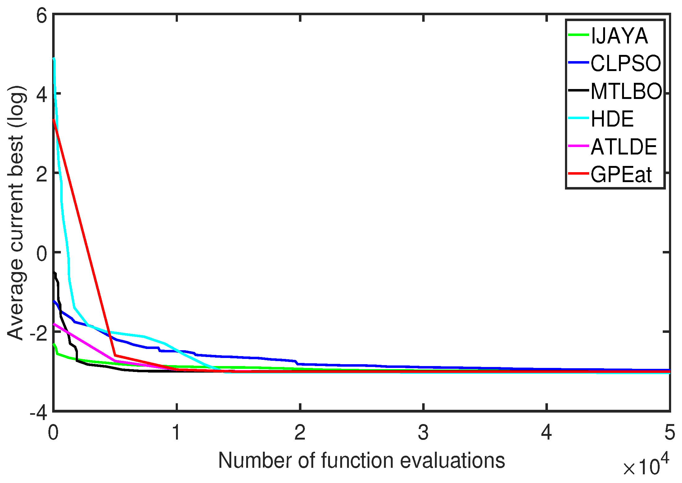
Figure 10 illustrates the convergence curves of six of these algorithms on the Photowatt-PWP201 model. It can be observed from the figure that GPEat converges at an exceedingly rapid rate, achieving an optimal solution in only 5000 FEs. In addition, the current–voltage characteristic curves based on the parameters identified by GPEat on Photowatt-WP201, STM6-40/36, and STP6-120/36 MM are shown in Figure 7c–e, respectively. These curves indicate that GPEat also performs well on these complex models.

In conclusion, in the five experiments, GPEat was able to accurately perform parameter estimation and find the optimal solution set. When compared with 11 algorithms, in the four indicators of the minimum RMSE value, maximum RMSE value, average RMSE value, and stability after 30 runs, it always ranked second or third, and sometimes even first. The standard deviation (std) of the algorithm’s output results is the core indicator for measuring its robustness. The smaller the std variation of the algorithm, the better its robustness. We observe that in the five related algorithm experiments of solar energy parameters, the changes in various std values are not significant. For example, the five std values of MTLBO are as follows: 1.9092749355 $\times {10}^{-17}$, 1.4395895110 $\times {10}^{-4}$, 1.3070106882 $\times {10}^{-17}$, 4.6260068533 $\times {10}^{-18}$, and 8.0041381348 $\times {10}^{-17}$, while the five std values of GPEat are 2.0033222035 $\times {10}^{-17}$, 1.2729158018 $\times {10}^{-6}$, 1.5590895357 $\times {10}^{-17}$, 6.5599406605 $\times {10}^{-18}$, and 7.7278995284 $\times {10}^{-17}$. Further analysis reveals that the std values of GPEat are concentrated in the range of $\times {10}^{-18}$ to $\times {10}^{-6}$, while the fluctuation range of MTLBO is from $\times {10}^{-18}$ to $\times {10}^{-4}$. Although the lowest std value of MTLBO (4.6260068533 $\times {10}^{-18}$) is slightly better than that of GPEat (6.5599406605 $\times {10}^{-18}$), its high fluctuation range ($\times {10}^{-4}$) is significantly larger than that of GPEat ($\times {10}^{-6}$), indicating that the output stability of MTLBO is more affected by the complexity of the problem, while GPEat is generally more robust in the estimation of PV model parameters and is more superior. From the above experimental results, compared with other optimization algorithms (including the current leading algorithms in solar PV model parameter estimation), GPEat has a better performance or competitiveness in terms of accuracy, stability, and speed, and it has a stronger overall capability.

5. Conclusions

In this article, we introduce an algorithm named gray predictive evolution with adaptive threshold adjustment strategy (GPEat) designed for parameter estimation across various PV models. GPEat incorporates dual mutation operators with synergistic effects, enhancing the algorithm’s capability to tackle intricate challenges. Additionally, an innovative adaptive threshold adjustment strategy is formulated within GPEat. This strategy is pivotal for selecting the appropriate mutation operator for each individual, ensuring a harmonious balance between maintaining genetic diversity within the population and achieving convergence. Detailed experimental analyses were carried out on multiple PV models, demonstrating that GPEat surpasses competing algorithms in terms of both precision and robustness. In the following, we summarize the key takeaways and contributions of this work:

GPEat consistently achieved lower Root Mean Square Error (RMSE) values across all tested PV models, indicating superior accuracy in parameter estimation. For instance, in the SDM, GPEat obtained an average RMSE of 9.8602187789 $\times {10}^{-4}$, outperforming algorithms such as IJAVA, ATLDE, and RLRTLBO. GPEat exhibited faster convergence rates, reaching optimal solutions in fewer function evaluations (FEs) compared to its counterparts. This acceleration is attributed to the adaptive threshold adjustment strategy (ATS), which dynamically selects appropriate reproduction operators based on the dimensionality of the problem. GPEat demonstrated robust performance across models of varying complexity, from the simple SDM to the more intricate DDM and MM. The algorithm’s ability to adapt its search strategy based on the feasible region lengths of decision variables ensured consistent performance, regardless of model complexity. The introduction of ATS significantly improved the performance of the base GPE algorithm. By adapting the threshold parameter proportionally to the length of each dimensional variable, ATS enabled GPEat to better handle the diverse search spaces encountered in PV model parameter estimation. This led to enhanced search efficiency, reduced likelihood of getting trapped in local optima, and ultimately, more accurate parameter estimates. GPEat excelled in scenarios where the feasible regions of decision variables varied significantly. Its adaptive nature allowed it to dynamically adjust its search strategy, outperforming other methods in complex, multi-modal search spaces, while GPEat demonstrated strong performance in most cases, it may encounter difficulties in extremely high-dimensional or highly constrained problems where the feasible regions are extremely narrow or fragmented. Future work should explore strategies to further enhance GPEat’s adaptability in such challenging scenarios.

One promising avenue for future research is the application of GPEat to Maximum Power Point Tracking (MPPT) control in PV systems. By accurately estimating PV model parameters, GPEat could potentially improve the efficiency and stability of MPPT algorithms under varying environmental conditions. In our future research, the adaptive threshold adjustment strategy will be applied to improve various advanced algorithms for solving various application problems. For PV model parameter estimation, we should note the variability in the length of different dimensions, which can be targeted to algorithm design to achieve more accurate performance prediction. At the same time, researchers can also optimize and adjust the formula of the adaptive threshold strategy and combine different advanced algorithms to solve more complex application engineering problems.

References

1. Xiong, G.; Zhang, J.; Yuan, X.; Shi, D.; He, Y.; Yao, G. Parameter extraction of solar photovoltaic models by means of a hybrid differential evolution with whale optimization algorithm. Sol. Energy 2018, 176, 742–761. [Google Scholar] [CrossRef]
2. Abdulla, H.; Sleptchenko, A.; Nayfeh, A. Photovoltaic systems operation and maintenance: A review and future directions. Renew. Sustain. Energy Rev. 2024, 195, 114342. [Google Scholar] [CrossRef]
3. Ayodele, T.; Ogunjuyigbe, A.; Ekoh, E. Evaluation of numerical algorithms used in extracting the parameters of a single-diode photovoltaic model. Sustain. Energy Technol. Assessments 2016, 13, 51–59. [Google Scholar] [CrossRef]
4. Babu, T.S.; Ram, J.P.; Sangeetha, K.; Laudani, A.; Rajasekar, N. Parameter extraction of two diode solar PV model using Fireworks algorithm. Sol. Energy 2016, 140, 265–276. [Google Scholar] [CrossRef]
5. Khanna, V.; Das, B.; Bisht, D.; Singh, P.K. A three diode model for industrial solar cells and estimation of solar cell parameters using PSO algorithm. Renew. Energy 2015, 78, 105–113. [Google Scholar] [CrossRef]
6. Jordehi, A.R. Parameter estimation of solar photovoltaic (PV) cells: A review. Renew. Sustain. Energy Rev. 2016, 61, 354–371. [Google Scholar] [CrossRef]
7. Olayiwola, T.N.; Hyun, S.H.; Choi, S.J. Photovoltaic modeling: A comprehensive analysis of the I–V characteristic curve. Sustainability 2024, 16, 432. [Google Scholar] [CrossRef]
8. Wang, G.; Zhao, K.; Shi, J.; Chen, W.; Zhang, H.; Yang, X.; Zhao, Y. An iterative approach for modeling photovoltaic modules without implicit equations. Appl. Energy 2017, 202, 189–198. [Google Scholar] [CrossRef]
9. Chen, Y.; Wang, X.; Li, D.; Hong, R.; Shen, H. Parameters extraction from commercial solar cells I–V characteristics and shunt analysis. Appl. Energy 2011, 88, 2239–2244. [Google Scholar] [CrossRef]
10. Gray, F.M.; Schmidt, M. A hybrid approach to thermal building modelling using a combination of Gaussian processes and grey-box models. Energy Build. 2018, 165, 56–63. [Google Scholar] [CrossRef]
11. Aslam, M.N.; Shaukat, N.; Asghar, Z. A novel heuristic-based physics-informed neural networks (H-PINNs)-based analysis of boundary stresses on magnetohydrodynamic convective flow in a convergent/divergent channel. Eur. Phys. J. Plus 2025, 140, 574. [Google Scholar] [CrossRef]
12. Cai, S.; Mao, Z.; Wang, Z.; Yin, M.; Karniadakis, G.E. Physics-informed neural networks (PINNs) for fluid mechanics: A review. Acta Mech. Sin. 2021, 37, 1727–1738. [Google Scholar] [CrossRef]
13. Gao, S.; Wang, K.; Tao, S.; Jin, T.; Dai, H.; Cheng, J. A state-of-the-art differential evolution algorithm for parameter estimation of solar photovoltaic models. Energy Convers. Manag. 2021, 230, 113784. [Google Scholar] [CrossRef]
14. Xiong, Y.; Luo, Y.; Peng, J.; Zhang, Q.; Huang, S. An improved population segmentation-based multi-mutation differential evolution algorithm for parameter extraction of photovoltaic models. Energy Convers. Manag. 2025, 327, 119553. [Google Scholar] [CrossRef]
15. Ishaque, K.; Salam, Z.; Mekhilef, S.; Shamsudin, A. Parameter extraction of solar photovoltaic modules using penalty-based differential evolution. Appl. Energy 2012, 99, 297–308. [Google Scholar] [CrossRef]
16. Qaraad, M.; Amjad, S.; Hussein, N.K.; Farag, M.; Mirjalili, S.; Elhosseini, M.A. Quadratic interpolation and a new local search approach to improve particle swarm optimization: Solar photovoltaic parameter estimation. Expert Syst. Appl. 2024, 236, 121417. [Google Scholar] [CrossRef]
17. Lu, Y.; Liang, S.; Ouyang, H.; Li, S.; Wang, G.g. Hybrid multi-group stochastic cooperative particle swarm optimization algorithm and its application to the photovoltaic parameter identification problem. Energy Rep. 2023, 9, 4654–4681. [Google Scholar] [CrossRef]
18. Saadaoui, D.; Elyaqouti, M.; Assalaou, K.; Lidaighbi, S.; Arjdal, E.; Choulli, I.; Elhammoudy, A.; Abazine, I. A hybrid optimization algorithm to identify unknown parameters of photovoltaic models under varying operating conditions. Eng. Appl. Artif. Intell. 2024, 133, 108544. [Google Scholar] [CrossRef]
19. Taleshian, T.; Malekzadeh, M.; Sadati, J. Parameters identification of photovoltaic solar cells using FIPSO-SQP algorithm. Optik 2023, 283, 170900. [Google Scholar] [CrossRef]
20. Rao, R.V.; Savsani, V.J.; Vakharia, D. Teaching–learning-based optimization: An optimization method for continuous non-linear large scale problems. Inf. Sci. 2012, 183, 1–15. [Google Scholar] [CrossRef]
21. Mirjalili, S.; Mirjalili, S.M.; Lewis, A. Grey wolf optimizer. Adv. Eng. Softw. 2014, 69, 46–61. [Google Scholar] [CrossRef]
22. Wang, H.; Yu, X.; Lu, Y. A reinforcement learning-based ranking teaching-learning-based optimization algorithm for parameters estimation of photovoltaic models. Swarm Evol. Comput. 2025, 93, 101844. [Google Scholar] [CrossRef]
23. Hu, Z.; Xu, X.; Su, Q.; Zhu, H.; Guo, J. Grey prediction evolution algorithm for global optimization. Appl. Math. Model. 2020, 79, 145–160. [Google Scholar] [CrossRef]
24. Dai, C.; Hu, Z.; Li, Z.; Xiong, Z.; Su, Q. An improved grey prediction evolution algorithm based on topological opposition-based learning. IEEE Access 2020, 8, 30745–30762. [Google Scholar] [CrossRef]
25. Xiang, X.; Su, Q.; Hu, Z. Non-equidistant grey prediction evolution algorithm: A mathematical model-based meta-heuristic technique. Swarm Evol. Comput. 2023, 78, 101276. [Google Scholar] [CrossRef]
26. Tong, W.; Liu, D.; Hu, Z.; Su, Q. Hybridizing genetic algorithm with grey prediction evolution algorithm for solving unit commitment problem. Appl. Intell. 2023, 53, 19922–19939. [Google Scholar] [CrossRef]
27. Xiang, X.; Su, Q.; Huang, G.; Hu, Z. A simplified non-equidistant grey prediction evolution algorithm for global optimization. Appl. Soft Comput. 2022, 125, 109081. [Google Scholar] [CrossRef]
28. Gao, C.; Hu, Z.; Xiong, Z.; Su, Q. Grey prediction evolution algorithm based on accelerated even grey model. IEEE Access 2020, 8, 107941–107957. [Google Scholar] [CrossRef]
29. Gao, C.; Hu, Z.; Miao, Y.; Zhang, X.; Su, Q. Four adaptive grey prediction evolution algorithms with different types of parameters setting techniques. Soft Comput. 2022, 26, 9247–9271. [Google Scholar] [CrossRef]
30. Oliva, D.; Abd El Aziz, M.; Hassanien, A.E. Parameter estimation of photovoltaic cells using an improved chaotic whale optimization algorithm. Appl. Energy 2017, 200, 141–154. [Google Scholar] [CrossRef]
31. Wei, H.; Cong, J.; Lingyun, X.; Deyun, S. Extracting solar cell model parameters based on chaos particle swarm algorithm. In Proceedings of the 2011 International Conference on Electric Information and Control Engineering, Wuhan, China, 15–17 April 2011; pp. 398–402. [Google Scholar]
32. Storn, R.; Price, K. Differential evolution–a simple and efficient heuristic for global optimization over continuous spaces. J. Glob. Optim. 1997, 11, 341–359. [Google Scholar] [CrossRef]
33. Kennedy, J.; Eberhart, R. Particle swarm optimization. In Proceedings of the ICNN’95-International Conference on Neural Networks, Perth, WA, Australia, 27 November–1 December 1995; Volume 4, pp. 1942–1948. [Google Scholar]
34. Zhang, J.; Sanderson, A.C. JADE: Adaptive differential evolution with optional external archive. IEEE Trans. Evol. Comput. 2009, 13, 945–958. [Google Scholar] [CrossRef]
35. Qin, A.K.; Huang, V.L.; Suganthan, P.N. Differential evolution algorithm with strategy adaptation for global numerical optimization. IEEE Trans. Evol. Comput. 2008, 13, 398–417. [Google Scholar] [CrossRef]
36. Zhan, Z.H.; Zhang, J.; Li, Y.; Chung, H.S.H. Adaptive particle swarm optimization. IEEE Trans. Syst. Man Cybern. Part B (Cybern.) 2009, 39, 1362–1381. [Google Scholar] [CrossRef]
37. Yu, Y.; Wang, K.; Zhang, T.; Wang, Y.; Peng, C.; Gao, S. A population diversity-controlled differential evolution for parameter estimation of solar photovoltaic models. Sustain. Energy Technol. Assessments 2022, 51, 101938. [Google Scholar] [CrossRef]
38. Marion, B.; Deceglie, M.G.; Silverman, T.J. Analysis of measured photovoltaic module performance for Florida, Oregon, and Colorado locations. Sol. Energy 2014, 110, 736–744. [Google Scholar] [CrossRef]
39. Li, S.; Gong, W.; Yan, X.; Hu, C.; Bai, D.; Wang, L.; Gao, L. Parameter extraction of photovoltaic models using an improved teaching-learning-based optimization. Energy Convers. Manag. 2019, 186, 293–305. [Google Scholar] [CrossRef]
40. Tong, N.T.; Pora, W. A parameter extraction technique exploiting intrinsic properties of solar cells. Appl. Energy 2016, 176, 104–115. [Google Scholar] [CrossRef]
41. Askarzadeh, A.; Rezazadeh, A. Parameter identification for solar cell models using harmony search-based algorithms. Sol. Energy 2012, 86, 3241–3249. [Google Scholar] [CrossRef]
42. Brest, J.; Greiner, S.; Boskovic, B.; Mernik, M.; Zumer, V. Self-adapting control parameters in differential evolution: A comparative study on numerical benchmark problems. IEEE Trans. Evol. Comput. 2006, 10, 646–657. [Google Scholar] [CrossRef]
43. Wang, D.; Sun, X.; Kang, H.; Shen, Y.; Chen, Q. Heterogeneous differential evolution algorithm for parameter estimation of solar photovoltaic models. Energy Rep. 2022, 8, 4724–4746. [Google Scholar] [CrossRef]
44. Li, S.; Gong, W.; Wang, L.; Yan, X.; Hu, C. A hybrid adaptive teaching–learning-based optimization and differential evolution for parameter identification of photovoltaic models. Energy Convers. Manag. 2020, 225, 113474. [Google Scholar] [CrossRef]
45. Abdel-Basset, M.; Mohamed, R.; Chakrabortty, R.K.; Sallam, K.; Ryan, M.J. An efficient teaching-learning-based optimization algorithm for parameters identification of photovoltaic models: Analysis and validations. Energy Convers. Manag. 2021, 227, 113614. [Google Scholar] [CrossRef]
46. Tanabe, R.; Fukunaga, A.S. Improving the search performance of SHADE using linear population size reduction. In Proceedings of the 2014 IEEE Congress on Evolutionary Computation (CEC), Beijing, China, 6–11 July 2014; pp. 1658–1665. [Google Scholar]
47. Yu, K.; Liang, J.; Qu, B.; Chen, X.; Wang, H. Parameters identification of photovoltaic models using an improved JAYA optimization algorithm. Energy Convers. Manag. 2017, 150, 742–753. [Google Scholar] [CrossRef]
48. Liang, J.J.; Qin, A.K.; Suganthan, P.N.; Baskar, S. Comprehensive learning particle swarm optimizer for global optimization of multimodal functions. IEEE Trans. Evol. Comput. 2006, 10, 281–295. [Google Scholar] [CrossRef]
Figure 1. Equivalent circuit diagram of SDM.
Mathematics 13 02503 g001
Figure 2. Equivalent circuit diagram of DDM.
Mathematics 13 02503 g002
Figure 3. Equivalent circuit diagram of TDM.
Mathematics 13 02503 g003
Figure 4. Equivalent circuit diagram of MM.
Mathematics 13 02503 g004
Figure 5. Convergence curves of GPEat and GPEnat on the STM640/36 model.
Mathematics 13 02503 g005
Figure 6. The usage of gray prediction operator for GPEat and GPEnat on the STM640/36 model.
Mathematics 13 02503 g006
Figure 7. The curves of simulated and measured data for (a) SDM, (b) DDM, (c) Photowatt-PWP201 MM, (d) STM6-40/36 MM, and (e) STP6-120/36 MM.
Mathematics 13 02503 g007
Figure 8. Convergence curves of compared algorithms for the single-diode model.
Mathematics 13 02503 g008
Figure 9. Convergence curves of compared algorithms for the double-diode model.
Mathematics 13 02503 g009
Figure 10. Convergence curves of compared algorithms for the Photowatt-PWP201 MM.
Mathematics 13 02503 g010