Research on Financial Stock Market Prediction Based on the Hidden Quantum Markov Model

Abstract

Quantum finance, as a key application scenario of quantum computing, showcases multiple significant advantages of quantum machine learning over traditional machine learning methods. This paper first aims to overcome the limitations of the hidden quantum Markov model (HQMM) in handling continuous data and proposes an innovative method to convert continuous data into discrete-time sequence data. Second, a hybrid quantum computing model is developed to forecast stock market trends. The model was used to predict 15 stock indices from the Shanghai and Shenzhen Stock Exchanges between June 2018 and June 2021. Experimental results demonstrate that the proposed quantum model outperforms classical algorithmic models in handling higher complexity, achieving improved efficiency, reduced computation time, and superior predictive performance. This validation of quantum advantage in financial forecasting enables the practical deployment of quantum-inspired prediction models by investors and institutions in trading environments. This quantum-enhanced model empowers investors to predict market regimes (bullish/bearish/range-bound) using real-time data, enabling dynamic portfolio adjustments, optimized risk controls, and data-driven allocation shifts.

1. Introduction

With the rapid advancement of econometric finance, the financial industry faces significant challenges due to the exponential growth of data and the increasing complexity of financial models. To address these issues, numerous mathematical models have been developed and applied in the financial sector. While numerous mathematical approaches address these issues, their computational demands and inherent limitations underscore the need for innovative solutions.

For instance, reference [1] offers a framework for families to calculate their asset portfolios, serving as a valuable guide for many family asset managers. However, as the volume of data continues to increase, these methods have become somewhat overshadowed in recent years. In response to these challenges, artificial intelligence (AI) and machine learning (ML) [2,3] have emerged as powerful tools for navigating the demands of the modern data-driven era. Extensive research has been conducted in this domain. For example, Ayyildiz and Iskenderoglu [4] introduced ML algorithms to predict movement trends of stock market indices in developed economies. While traditional machine learning methods demonstrate promise in stock index prediction, their scalability is constrained by exponentially growing data volumes. Consequently, quantum computing has emerged as a transformative solution to overcome these limitations by leveraging its computational efficiency advantages.

This paper introduces a novel stock prediction framework that employs a GMM-MVTF (Gaussian mixture models and means and variances to feature) discretization pipeline to overcome the inherent limitations of Gaussian mixture models (GMM) in handling continuous data for stock market predictions. By using the Shanghai Stock Exchange (SSE) and Shenzhen Stock Exchange (SZSE) datasets, this paper evaluates three HQMM variants: one with MVTF-discretized data and another with evenly discretized data, with performance comparisons against classical HMM under distinct processing techniques. This study unlocks a new dimension of quantum-enhanced computing for the industry and provides a valuable reference for further investigating the potential applications of quantum algorithms in other fields.

2. Related Work

2.1. Classical Machine Learning in Finance

Early ML applications focused on enhancing financial decision-making. Mahmoodi et al. [5] focused on using these algorithms to accurately forecast stock trading signals in financial markets. These studies highlight the immense potential of AI and ML in the financial sector, particularly in enhancing decision-making processes and improving portfolio management performance. Investing in stocks is a widely used strategy for portfolio diversification. However, it requires consideration of numerous factors, and individuals often encounter huge challenges when selecting stocks outside their areas of expertise. Identifying the most relevant factors for different stocks and addressing the biases introduced by specialized professional domains are necessary. Previous studies have made notable contributions to these issues. For example, Stambaugh [6] proposed a regression approach to investigate the relationship between lagged return rates and random regression quantities, which provides a viable framework for predicting and reporting various investment strategies and is able to mitigate regression interference brought by innovative regression quantities. Endri et.al. [7] aimed to develop an early warning system (EWS) model for predicting the delisting risk exposure of Islamic equities (ISSl) using a Support Vector Machine (SVM) with a set of financial variables. By optimizing SVM hyperparameters and employing hybrid architectures (e.g., SVM-deep learning), the model enhances predictive robustness, demonstrating the predictive power of financial indicators for delisting risk. Although AI and ML have proven to be valuable tools in stock market applications, researchers have observed that the computational power consumption of traditional ML methods has increased with the growing volume of market data [8]. Therefore, it is essential to explore other effective approaches to address the escalating consumption of data and computational resources.

2.2. Quantum Computing Approaches

Quantum methods demonstrate theoretical superiority in financial modeling. Due to its unique advantages of novel and efficient technology, quantum computing has emerged as an updated alternative to tackle existing challenges [9,10,11]. Jeswal and Chakraverty [12] stated that quantum neural networks are superior to classical methods across multiple domains such as SORNETTE, which explores a variety of models constructed based on the Ising model and extends them to elucidate numerous stylized features in financial markets, and Bagheri et al. utilized the Quantum-behaved Particle Swarm Optimization (QPSO) algorithm to optimize the membership functions of the Adaptive Network-based Fuzzy Inference System (ANFIS) for forecasting financial time series, particularly in the foreign exchange market [13,14]. As a fundamental statistical method in time-series analysis, the hidden Markov model (HMM) is now playing a pivotal role in the stock market by considering its various hidden characteristics. Early in 2011, Guidolin [15] comprehensively reviewed the applications of the Markov transformation models in empirical finance, such as the analyses of stock returns, the term structure of default-free interest rates, the dynamics of exchange rates, and the joint process of stock and bond returns. Based on the quantum conditional master equation, a new quantum ML algorithm, split hidden quantum Markov model (SHQMM), was proposed by Li et al. [16,17], which further expands the potential applications of quantum computing in complex systems.

While HQMM [18] theoretically addresses these gaps, no prior work has implemented them for stock prediction due to the unsolved challenge of continuous data discretization. Against the backdrop of growing research interest in quantum machine learning for financial time-series problems, this paper proposes a quantum-based prediction algorithm for the stock market, built upon the HQMM. Leveraging the unique characteristics of quantum computation, the proposed HQMM-based algorithm is compared with the classical HMM to highlight the advantages of quantum coherence. The study involves data collection and processing and addresses the limitations of handling continuous data through Gaussian mixture models (GMM) and means and variances to feature (MVTF) analysis. Model training likelihood function is constructed based on temporal features. The model is evaluated and optimized using the distance and accuracy (DA) algorithm, thereby enabling the systematic demonstration of AI quantitative algorithms’ applied value in accelerating model training, autotuning hyperparameters, enhancing feature retention, dynamically adapting to trading environments, and generating investment-actionable insights.

3. The Comparison Between the Classical HMM and HQMM

3.1. Hidden Markov Model in Stock Forecasting

HMM describes a hidden Markov chain that generates an unobservable sequence of states, where the state probability at time t, $P\left(y_t\right)$, is only determined by the previous state $y_{t-1}$, as (1) shows:

$$P(y_t|y_{t-1},y_{t-2},\dots ,y_t)=p(y_t|y_{t-1})$$

(1)

By using the time-independent constant matrices A and C to define the transition matrix and the observation matrix, respectively, in the Markov process, the model can be defined as $\lambda =\left(\mathit{A}, \mathit{C}, \mathit{\pi }\right)$ [19], which denotes the initial state distribution $\mathit{\pi }$ [20]:

$$\mathit{A}={[a_{i,j}]}_{N\times N}$$

(2)

$$\mathit{C}={[c_{i,j}]}_{N\times M}$$

(3)

$$\mathit{\pi }={[{\pi }_i]}_N$$

(4)

where there are the elements at the i-th row and the j-th column of the N × N transition matrix and the N × M observation matrix, respectively. The initial state distribution ${\mathit{\pi }}_i$ defines the probability of being in state i at the first time point. When the HMM is applied to stock market prediction, elements such as the risk-free interest rate, systemic risk, and risk premium are incorporated into the hidden state, and the observation matrix represents the price of each stock. By using historical daily stock prices as input data, the transition matrix A and observation matrix C of HMM are trained by using ML techniques. Then, the probability of each subsequent hidden state can be derived from matrix A, while the probability of the most possible stock price at the next time step [19,21] can be calculated using the following equation:

$${\delta }_{t+1}(i)={\max }_{1\le j\le N}[{\delta }_t(j)a_{j,i}]c_i(o_{t+1})$$

(5)

Given model $\lambda =\left(\mathit{A}, \mathit{C}, \mathit{\pi }\right)$ and observation sequence = {$o$₁, $o$₂, … $o$_T}, $o_{t+1}$ is the observation vector $o$ at time t + 1, where ${\delta }_{t+1}(i)$ is the predicted state with the largest probability at time t + 1. Obviously, this model only focuses on the price variations of a single stock over time but ignores other influencing factors. However, in the real stock market, numerous factors have a determinant influence on stock prices, including both external and internal variables, such as risk-free interest rate, systemic risk, and risk premium. This renders HMM-based predictions fundamentally unstable in real environments.

3.2. Hidden Quantum Markov Model

As an extension of the classical HMM framework, HQMM [22] can be expressed as follows:

$$p(y_t|{\rho }_{t-1})=\mathrm{tr}(K_{y_{t-1}}{\rho }_{t-1}{K}_{y_{t-1}}^{†})$$

(6)

$${\rho }_t={\displaystyle \frac{K_{y_{t-1}}{\rho }_{t-1}{K}_{y_{t-1}}^{†}}{\mathrm{tr}(K_{y_{t-1}}{\rho }_{t-1}{K}_{y_{t-1}}^{†})}}$$

(7)

where $y_t$ is the observation state, ${\rho }_{t-1}$ is the known state, $p(y_t|{\rho }_{t-1})$ is the conditional probability of the observation state at time t when the density matrix $\rho$ at time $t-1$ is known, tr is the trace, $K_{y_{t-1}}$ is the Kraus operator corresponding to the observation state at time $t-1$, and the superscript $†$ indicates the conjugate.

HQMM is trained using gradient descent or variational inference to optimize quantum operators by density matrix ρ (showing the hidden state) and state update (controlled by the Kraus operator {Km}, following quantum channel constraints, where m is the number of the operator, and I refers to the identity matrix). Through the global information storage of quantum states, interference effects, long-term dependency modeling, and exponentially scalable state space, HQMM breaks through the limitations of HMM, which can only focus on a single stock trend, making it more suitable for multi-asset, market linkage analysis and intricate financial systems.

Both HMM and HQMM are capable of inferring the probability of the next state from the previous state. In a classical HMM, the next hidden state and observation state can be inferred from the transition matrix A and the state observation matrix C, respectively. Comparatively, in HQMM, the Kraus operator replaces the matrices A and C, serving to predict the next state. Traditional HMMs can only model Markov processes, where the current state depends solely on the previous state, and a fixed probability transition matrix governs transitions. In contrast, Kraus operators in HQMMs leverage density matrices to retain historical information and quantum coherence. Additionally, HQMMs allow the use of multiple Kraus operators, each of which can correspond to different market conditions or trading patterns, providing greater flexibility in capturing complex financial dynamics. A comparison of the two models is presented in

Table 1. The comparison between the classical HMM and HQMM [22].

HMM Probability		HQMM Analogue
Description	Representation	Description	Representation
Belief State	$\overrightarrow{x}$	Density Matrix	$\widehat{\rho }$
Joint Distribution	${\overrightarrow{x}}_1\otimes {\overrightarrow{x}}_2$	Multi-particle Density Matrix	$\widehat{\rho }{X}_1\otimes \widehat{\rho }{X}_2$
Marginalization	$\overrightarrow{x}={\displaystyle \sum _d\overrightarrow{x}\otimes \overrightarrow{d}}$	Partial Trace	$\widehat{\rho }X=t{r}_D(\widehat{\rho }XD)$
Conditional probability	$P(\overrightarrow{x}|d)={\displaystyle \frac{P(d,\overrightarrow{x})}{P(d)}}$	Projection + Partial Trace	$\begin{array}{l}P(state|d)=\\ t{r}_D({\widehat{P}}_d\widehat{\rho }XD{\widehat{P}}_d^{†})\end{array}$

, and the relevant formulas and characteristics can be found in Ref. [22].

In classical HMM probability, the vector $\overrightarrow{x}$ represents the probability of different market states and is referred to as a probability vector. The belief state reflects the confidence level in the market being in a specific state at a given moment—such as rising, stable, or falling. The joint distribution ${\overrightarrow{x}}_1\otimes {\overrightarrow{x}}_2$ encodes the combined probability of two or more variables occurring simultaneously. Marginalization $\overrightarrow{x}={\displaystyle \sum _d\overrightarrow{x}\otimes \overrightarrow{d}}$ refers to the process of ignoring a variable d in order to focus only on the distribution over x. Conditional probability $P(\overrightarrow{x}|d)={\displaystyle \frac{P(d,\overrightarrow{x})}{P(d)}}$ is used to update belief about x, given new information d.

In the HQMM analogue, $\widehat{\rho }$ represents a density matrix, which incorporates not only probabilistic information but also quantum coherence. Density matrix allows for interference between different states, making it more suitable for capturing the complexity of financial markets. A multi-particle density matrix, $\widehat{\rho }{X}_1\otimes \widehat{\rho }{X}_2$, models the joint behavior of strongly correlated variables—such as two closely linked sectors—more accurately. A partial trace, $\widehat{\rho }X=t{r}_D(\widehat{\rho }XD)$, is used when macro-level information (D) is known and focuses on a particular asset (X), obtaining partial trace for the macro-variable (D). Projection+partial trace constitutes the quantum analogue of conditional probability: the system is first projected onto a measured outcome d (e.g., a major policy announcement), and then a partial trace is taken to infer its effect on the market state X (e.g., stock movement).

Fundamentally, HMM and HQMM differ in their modeling approach. HMM forecasts market behavior by learning transition probabilities between historical price states. In contrast, HQMM leverages the principles of quantum mechanics—superposition (interference between rising and falling probabilities) and entanglement (interlinked behavior of assets like U.S. and Chinese stocks)—to potentially capture more intricate market dynamics. This includes nonlinear dependencies, long-range memory effects, and hidden correlations that classical models may fail to represent.

4. Experimental Procedure Introduction

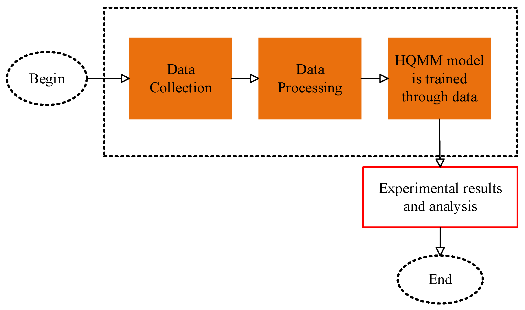
To achieve accurate prediction of the stock market based on HQMM, three main steps should be performed, involving the collection of real-time stock data, conversion of the continuous data into discretized formats, and training of HQMM based on the processed data to predict stock trends, as illustrated in Figure 1.

4.1. Data Collection

Here, 15 stocks with stock codes of 000901, 000036, 000031, 601318, 600519, 600009, 600004, 600050, 600022, 000623, 000401, 000488, 000518, 000800, and 000895 were taken into consideration. The 5 key indices of these stocks, opening price, highest price, lowest price, closing price, and trading volume, were collected daily from the real-time stock data of SSE and SZSE from June 2018 to June 2021. Financial data were accessed via the Tushare Application Programming Interface (API). The workflow integrates multiple specialized libraries: backtrader and Tushare for stock data acquisition, pandas and NumPy for data preprocessing, hmmlearn and scikit-learn for classical modeling (hidden Markov models and Gaussian methods), and Qiskit for quantum circuit implementation. The following data were split into different time periods: 1 June 2018–26 October 2019 (training period), 30 October 2019–24 August 2020 (validation period), and 24 August 2020–23 June 2021 (testing period).

Each stock has an index number of 5. These indices serve as the evaluation standards for investment performance and the innovation of index derivative products, providing the foundational conditions for index investment.

4.2. Data Processing

As discussed before, the current HQMM-based algorithm can only handle discretized time-series data [21]; thus, the obtained continuous data from SSE and SZSE cannot be directly used for this hidden quantum Markov prediction. To ensure that the data can be compatible with HQMM, further data processing is required. As for HMMs, when continuous data is applied, integrated algorithms, such as Gaussian HMM, are usually employed. However, an equivalent quantum version of such an approach is not accessible for HQMM, necessitating the exploration of alternative methods. Discretizing continuous data is often considered the first option for HQMM; however, it also faces a significant challenge. The original data may be seriously distorted, having a negative impact on the model’s effectiveness. As a result, another method—integrating the Gaussian mixture model (GMM) with the means and variances to feature (MVTF) model—is proposed and also applied for data processing, aiming at ensuring maximum fidelity in financial data representation and thus enhancing the model performance.

4.2.1. Even Discretization of Continuous Data

• In order to better discretize continuous data, the traditional discretization method in

  Table 2. Classify stock data into integers.

  Growth Rate	Rise	Down
  0~5	1	2
  5~10	3	4
  10~∞	5 (bull market)	6 (bear market)

  is presented, and then the experimental method in

  Table 3. According to the classification of the value of L, it is converted to the value of S.

  Range	Value of S	Range	Value of S
  −20 < L ≤ 0	1	0 < L ≤ 20	2
  −50 < L ≤ −20	3	20 < L ≤ 50	4
  L ≤ −50	5	L ≥ 50	6

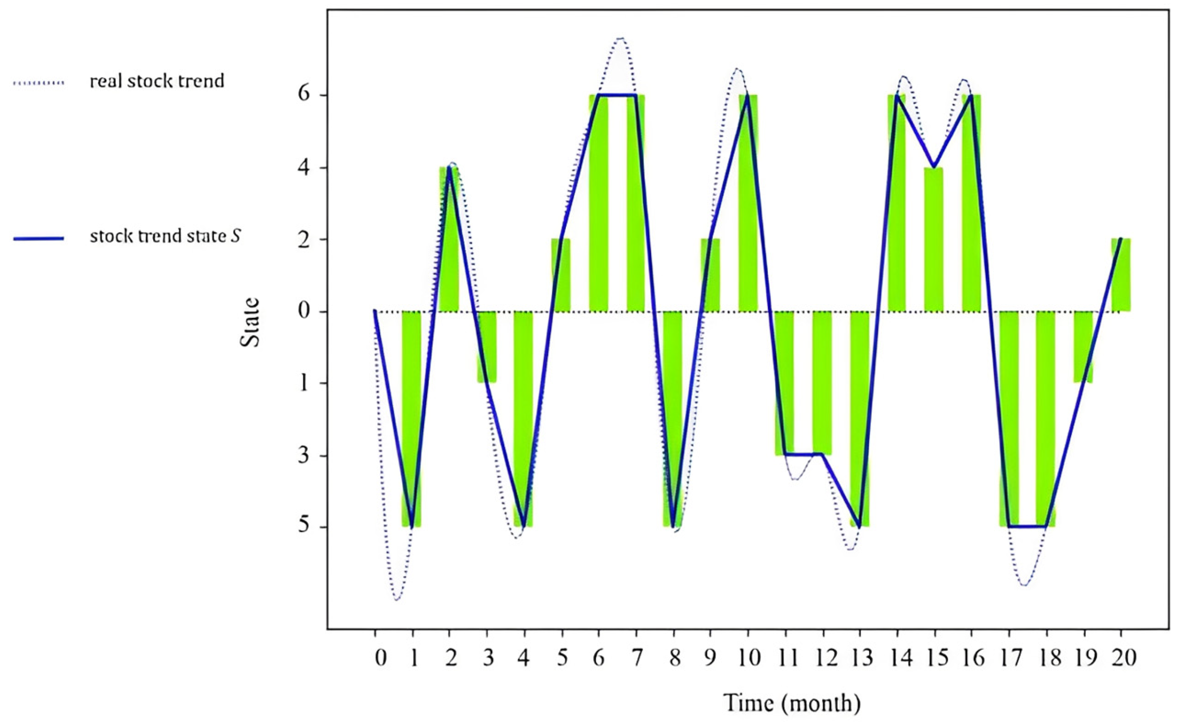
  is improved to reduce external interference. Table 2 demonstrates that the data underwent straightforward processing and were subsequently input into the HQMM model. While the prediction results were generated, they were significantly influenced by external factors, leading to a lack of robustness and vulnerability to artificial interference. To enable a fair comparison with our improved method, the same approach was employed, whereby the obtained data were categorized into three intervals based on stock price fluctuations. These intervals were represented by the integer values 1, 3, 5, 2, 4, and 6, respectively (Table 3). The value of L is mentioned in formula 8 (through the calculation of GMM mean and variance and MVTF below), and L is converted into the value of S(Observation status in Table 3) and then transformed into a bar graph in Figure 2. The ordinate of the green bar chart is the value of separate S, the dotted line represents the real stock trend value, and the solid line is the line of the midpoint of the bar chart, indicating that the stock trend obtained through the division of S is more realistic.

The calculation of stock price fluctuations (increase or decrease) is performed by subtracting the previous day’s closing price from the next day’s closing price. If the resulting value S is positive, it indicates a rise; conversely, a negative S signifies a fall. This approach facilitates the data input into the HQMM model and simplifies the subsequent analysis of experimental results.

4.2.2. Data Discretization with GMM and MVTF

The processing steps of our proposed method, which combines GMM with MVTF to discretize continuous data, are as follows:

(1) The data collected during a certain time period are first inputted into the GMM-based ML algorithm, allowing for the training of multiple Gaussian distributions. The common steps for GMM to process data are as follows: (i) The dataset and the variables to cluster are selected. (ii) The optimal cluster number K is determined based on the characteristics and size of the dataset using the Bayesian Information criterion (BIC) or Akaike Information criterion (AIC) through multiple experiments. The cluster parameter K is empirically determined as 6 in this experimental setup. (iii) Random initialization or k-means algorithm is used to initialize GMM parameters. (iv) The expectation maximization (EM) algorithm is used to assign each sample to the Gaussian distribution with the highest probability, and the probability of each sample belonging to the Gaussian distribution is calculated (posterior probability, E-step). (v) M-step in the EM algorithm is used to find the mean value, method, and weight. (vi) Steps iv and v are repeated until the posterior probability change is less than a certain value. (vii) The mean and variance of each distribution are extracted based on the resulting distribution.

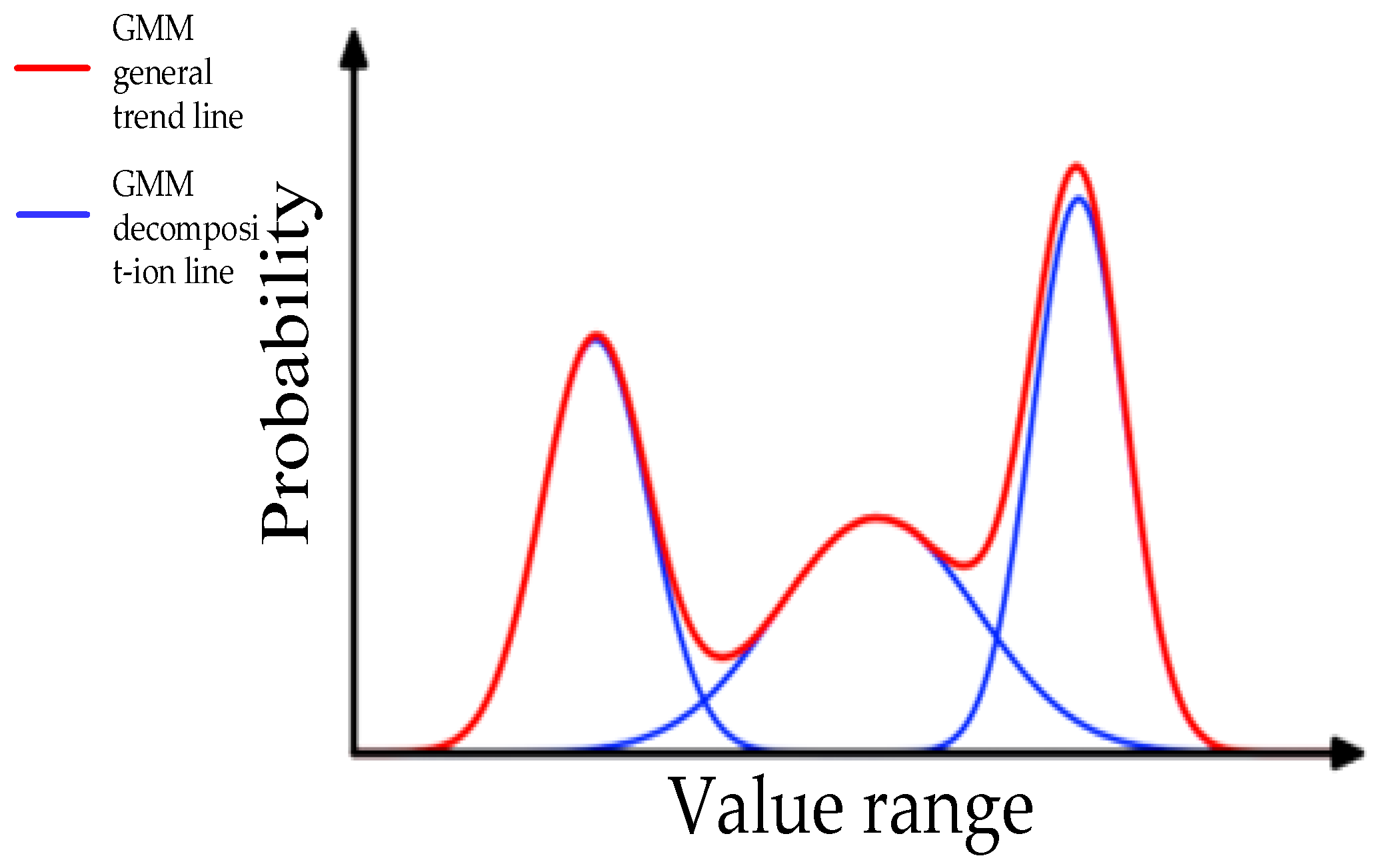
• In an experimental model, the collected data is accurately quantified and decomposed into k models based on the Gaussian probability density function, as shown in Figure 3. (Schematic diagram illustrates GMM, so no scale is required. The red line is the overall trend, which then breaks down into the blue line). Here, a one-dimensional GMM is utilized, the 30-day data is considered and input into a Gaussian mixture model for training, and n is set to 5, where n represents the number of Gaussian mixture components. In order to ensure consistent generalization across all data samples and to avoid the imbalance phenomenon where some data perform exceptionally well while other data significantly deteriorate due to parameter deviations, the above parameters were selected. This means that the GMM model learns five Gaussian distributions and obtains variances (${\sigma }_1,{\sigma }_2,\cdots ,{\sigma }_5$) and means (${\mu }_1,{\mu }_2,\cdots ,{\mu }_5$) of these Gaussian distributions.

(2) The means and variances obtained in the previous step are further processed through the MVTF model and then used to determine the trend states of the stocks over the specified period. During this step, how to convert the before-derived means and variances into the stock trend states (indicating a bull or bear market) is crucial because it has a significant effect on the fidelity degree of the experimental data when input into HQMM. To maximize this fidelity, the following conversion processes are performed:

• The n variances (${\sigma }_1,{\sigma }_2,\cdots ,{\sigma }_n$) obtained from the experimental data are sorted from small to large and assigned to $a_1,a_2,\cdots ,a_n$ in order, and the mean ${\mu }_i$ corresponding to ${\sigma }_i$ is also assigned to $b_1,b_2,\cdots ,b_n$ in the same order as $\mathsf{\sigma }$.
• The L value of each set of data is calculated using the following equation:

  $$\mathrm{L}={\displaystyle \sum _{i=1}^n{b}_i(i\ast 5\%+5\%)}$$

  (8)
• $b_i$ represents the mean ${\mu }_i$ corresponding to the i-th variance $a_i$. The trend state S of stocks can be defined by classifying the value of L (L is a calculated value based on $b_i$ and a weighting coefficient), based on the classification principle shown in Table 3. To ensure MVTF fully leverages all information from the GMM-generated Gaussian distributions while accounting for the correlation between experimental results and the number of Gaussians, Formula (8) is derived by using a criterion. As a result, the stock trend state S is made into tabular data. Correspondingly, the resulting trend state of stock 600519 is shown in Figure 2.

Besides the above processes involving GMM and MVTF, the whole operation flow of data processing also includes: (i) collecting real-time stock data; (ii) calculating and tabulating the difference between the closing price of each day and that of the previous day; (iii) splitting all collected data into a group of 30 days; (iv) inputting each group of data into GMM and setting the number of Gaussian distributions in GMM to n (n is an integer and n ≥ 1); (v) calculating the means and variances of n Gaussian distributions; and (iv) converting these means and variances into the stock trend state through the MVTF model. After these operations, the collected continuous financial market data is successfully discretized and finally converted into a format accessible to HQMM.

4.3. HQMM Training

In order to accurately predict the stock market with the previous data processing results, the HQMM model is constructed. How to construct the likelihood function and solve the Kraus operator with the gradient descent method is at the core of this model. The historical stock observation data $S_1,S_2,\dots ,S_n$ are used to construct the likelihood function [23] as follows:

$$\varsigma =\ln \mathrm{tr}(K_{S_n}\cdots (K_{S_1}{\mathit{\rho }}_0{K}_{S_1}^{†})\cdots K_{S_n}^{†})$$

(9)

where ${\mathit{\rho }}_0$ is the manually set initial density matrix. In the initial state ${\mathit{\rho }}_0$ under different K values, it exhibits the advantage of robustness, allowing the model state to evolve from any initial state to a stable state. Additionally, the manually set method for HQMM is the same used in References [16,23]. During the HQMM process, when the Markov chain has a long sequence, ${\mathit{\rho }}_0$ will produce a decoherence effect. In the process of evolving the relative state, for the first half of a batch, any initial state undergoes evolution, while the second half undergoes the experiment. In this experiment, ${\mathit{\rho }}_0$ can be set to the following: $\left(\begin{array}{cc} 8.0360857\hspace{0.33em}\times \hspace{0.33em}{10}^{-2}& -3.4289963\hspace{0.33em}\times \hspace{0.33em}{10}^{-2}\\ -3.4289963\hspace{0.33em}\times \hspace{0.33em}{10}^{-2}& 9.1963914\hspace{0.33em}\times \hspace{0.33em}{10}^{-1}\end{array}\right)$.

Then, the likelihood function (9) is used to calculate the derivative of all possible Kraus operators for gradient descent to maximize the value of the likelihood function. Therefore, a matrix solution to the Kraus operator $K_{S_n}$ is obtained, which is the n-th Kraus operation matrix. Each observation value corresponds to an operation matrix, which is the same at the beginning; the solution of the derived HQMM is transformed into a constrained optimization problem: relational matrix $\varsigma$ is the maximum and ${\displaystyle \sum K_m^{†}}{K}_m=I$ [24], with m being the number of the operator and I referring to the identity matrix. Then, the likelihood function is used to conduct derivative processing on all the Kraus algorithms. Subsequently, the gradient descent method is employed to calculate the maximum likelihood function value, thereby enabling the determination of the matrix solution of the first Kraus.

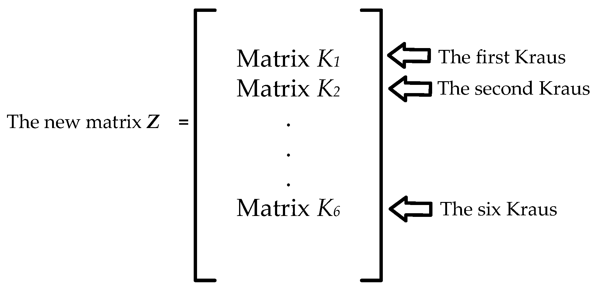
For the convenience of computer operation, a new matrix Z [24] is reconstructed by stacking all the $2\times 2$ Kraus operator matrices, as shown in Figure 4. It has a dimension of $2H\times 2$, determined by the output number H, i.e., the number of stock observation states. The constrained optimization problem requires the constructed matrix Z to satisfy the following: $\varsigma$ is the maximum and ${\mathit{Z}}_m^{†}{\mathit{Z}}_m=I$ [24]. Since $\mathit{Z}$ is on the Stiefel manifold, its constrained optimization problem can be transformed into the following unconstrained problem, which can be solved by the gradient descent algorithm: $G=\partial \varsigma /\partial Z$ [24] and $Z=Z-\tau \mathit{U}{\left[I+(\tau /2){\mathit{V}}^{†}\mathit{U}\right]}^{-1}{\mathit{V}}^{†}Z$ [24]. Here, G is the partial differential of the likelihood function for Z; $\tau$ is the step size of gradient descent (a real number in the interval [0, 1]); and both $\mathit{U}$ and ${\mathit{V}}^{†}$ are the augmented matrices and represented by $\left[\left.G\right|Z\right]$ and $\left[\left.Z\right|-G\right]$ [24]. By solving this constrained optimization problem, the Kraus operator can be solved, the latest ${\mathit{\rho }}_t$ is updated, and the whole HQMM is obtained. Finally, the result of reversing $\mathit{Z}$ to obtain the Kraus operators is derived, and the quantum hidden Markov model is used to solve and obtain the prediction of the stock’s trend, $\begin{array}{l}P(S_t\left|{\rho }_{t+1}\right.)\end{array}$, at the next moment, based on the results of the Kraus operators.

To accurately evaluate the model’s performance, the description accuracy (DA) must be obtained. The fundamental principle of DA is to serve as a standardized log-likelihood ratio metric. It achieves likelihood standardization with respect to state-space dimension and length normalization, enabling fair comparison across models of varying complexity. For more detailed explanations, refer to reference [22]. The algorithm is adopted and defined as follows:

$$\mathrm{DA}=f\left(1+{\displaystyle \frac{{\log }_{w}P(\left.Y\right|D)}{r}}\right)$$

(10)

where r is the length of the sequence, w is the number of hidden states, Y is the observation data, D is the generated model, and f (·) is a nonlinear function that takes the argument from (−∞, 1] to (−1, 1]:

$$f(x)=\left\{\begin{array}{l}x \hspace{1em}\hspace{1em}\hspace{1em}, x\ge 0\\ {\displaystyle \frac{1-{\mathrm{e}}^{-0.25x}}{1+{\mathrm{e}}^{-0.25x}}},x<0\end{array}\right.$$

(11)

If DA = 1, the model perfectly predicts the stochastic sequence, while 1 > DA $\ge$ 0 means that the model predicts the sequence better than random [22]. If DA < 0, the results indicate that the model performs poorly and is inferior to a random baseline. The more DA converges to 1, the better the model functions. It describes the DA as the loss function used to evaluate the quality of the model training. 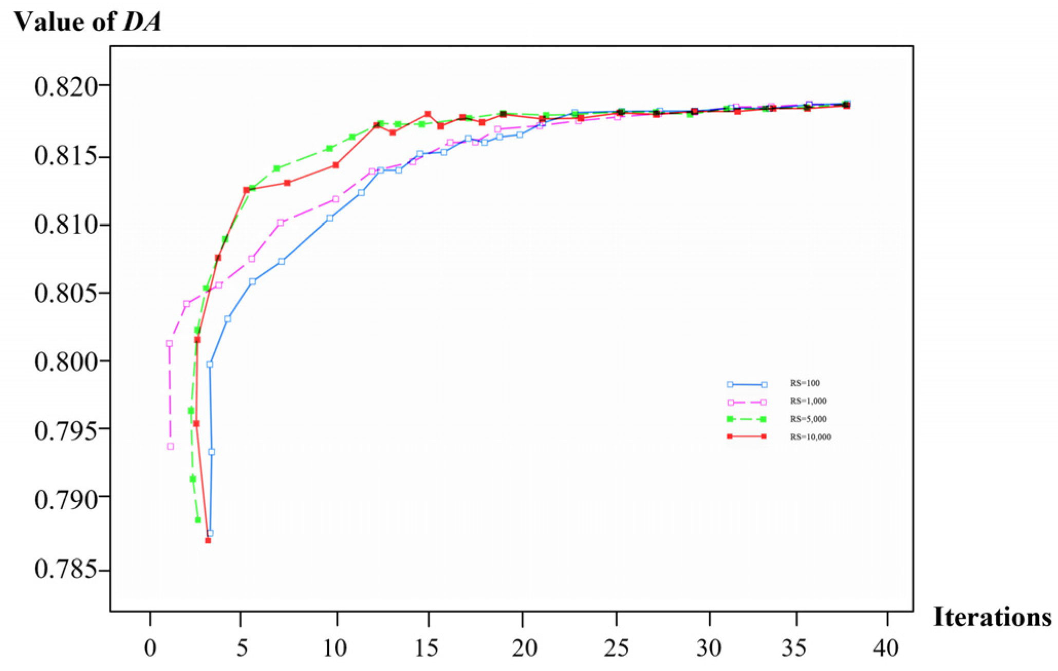In repeated experiments, DA demonstrates noise resistance in measurement, with its values eventually converging to a stable state [16]. Subsequently, through the model, the influence of different initialization positions of Kraus (equivalent to data noise) on the training results of the model is calculated, as shown in Figure 5 [16]. The RS represents the random number seed.

5. Experimental Results and Discussion

Since different stocks and lengths of prediction time would lead to different prediction performances for both HQMM and HMM, 15 distinct stocks were selected for analysis, and the average performance was calculated to evaluate the models’ performance. During the experiment, for the HQMM model constructed in this paper, the number of hidden states was 6, which was derived through global optimization, while the settings for the Kraus operators and density matrices were retained from prior configurations. This methodology ensures robustness and stability across the full dataset, thereby eliminating performance fluctuations induced by data distribution discrepancies. 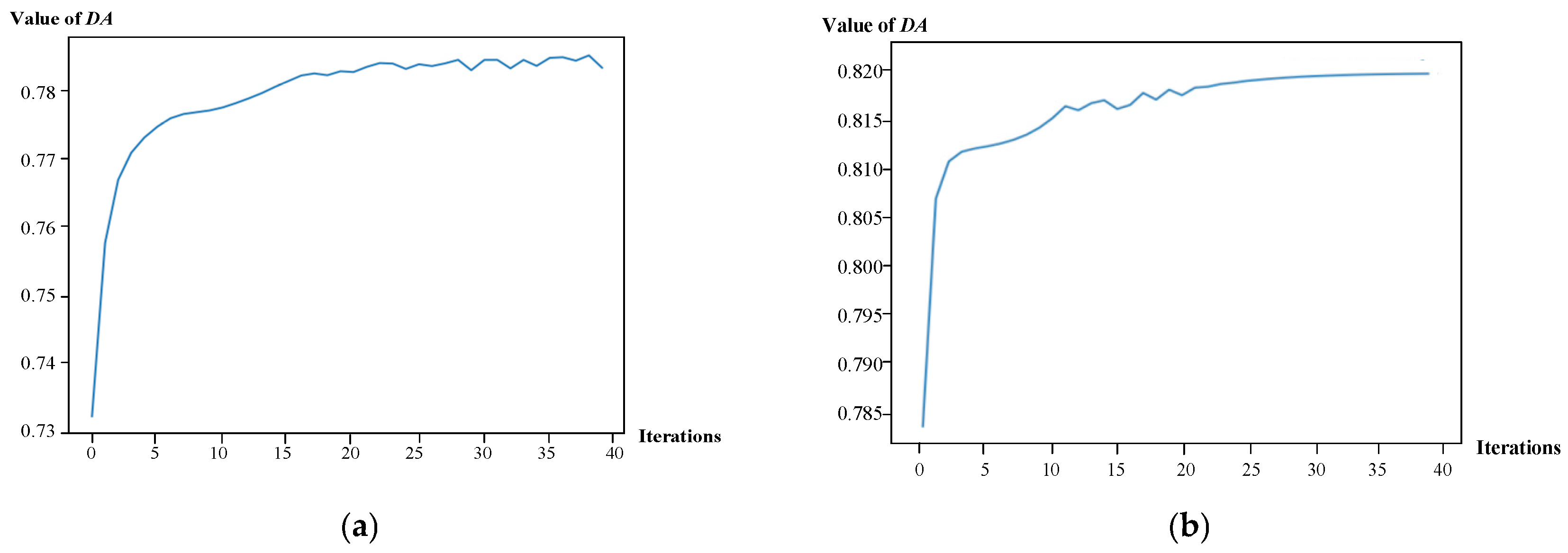Additionally, the matrix Z with a dimension of $12\times 2$ is obtained from the training process. The calculated results of DA for the evenly-discretized continuous data and that processed with MVTF are shown in Figure 6a,b, respectively. It can be found that when the number of iterations is less than 5, the value of DA increases rapidly, while once the number of iterations exceeds 40, the value of DA tends to converge. At this time, the mode training is completed.

Upon completing model training, the following steps are further conducted to investigate the model’s prediction performance:

• Based on the constructed matrix Z, six matrices ${\mathit{K}}_1,{\mathit{K}}_2,\cdots ,{\mathit{K}}_6$ are obtained, and the corresponding prediction values $J_1,J_2,\cdots ,J_6$ could be calculated by the following equation:

  $$J_n=-\ln \left[\mathrm{tr}\left({\mathit{K}}_n{\mathit{\rho }}_{\mathrm{t}}{\mathit{K}}_n^{†}\right)\right]$$

  (12)
• The minimum value $J_n^{\prime }$ is found among $J_1,J_2,\cdots ,J_6$, and thus the subscript $n \left(n\in \left[1, 6\right]\right)$ is the predicted state at the t time. For example, if the minimum value is $J_3^{\prime }$, 3 is the most possible next state (E).
• By setting the initial capital (IC) to 1,000,000, the trend of each stock is predicted one by one with different methods. If the prediction result of one stock is rising, i.e., $J_n^{\prime }$ is $J_2^{\prime }$, $J_4^{\prime }$, or $J_6^{\prime }$, buy(long) it; otherwise, sell(short) it. if the prediction result is falling ($J_n^{\prime }$ is $J_1^{\prime }$ $J_3^{\prime }$, or $J_5^{\prime }$). In order to measure the prediction effect, for the following scheme, the final capital (FC) that the operator (including buying and selling at the right time) uses for HQMM can be obtained. It should be noted that the transaction costs in the whole process are neglected. The core function of HQMM is to predict market state evolution by forecasting the most probable range of price fluctuations, and it is decoupled from trade execution. If HQMM needs to be integrated into a trading system for downstream applications, this can be achieved in the future through a portfolio optimization module.

To compare the prediction result of the stock with the natural growth capital (NC), the comparative growth rate (R) is proposed [25], formulated as follows:

$$R={\displaystyle \frac{\mathrm{FC}-\mathrm{NC}}{\mathrm{FC}}}\times 100\%$$

(13)

$$\mathrm{NC}=\mathrm{IC}\times \left(\mathrm{FP}/\mathrm{IP}\right)$$

(14)

$$\mathrm{FC}=\mathrm{FC}\times \left(\mathrm{SP}/\mathrm{BP}\right)$$

(15)

where IP is the initial price of each stock, FP is the final price of each stock at the time of experiment, SP is the selling price, and BP is the buying price. Obviously, NC can be obtained from the real data of the stock, as shown in

Table 4. Real trend of the stocks in a certain period.

Stock Code	Period (Day)	IC (CNY)	NC (CNY)	Change Rate
000901	90	1,000,000	1,716,216	71.62%
000036	90	1,000,000	1,359,855	35.98%
000031	90	1,000,000	1,384,458	38.44%
601318	90	1,000,000	1,391,863	39.18%
600519	90	1,000,000	1,409,882	40.98%
600009	180	1,000,000	1,290,323	29.03%
600004	180	1,000,000	1,516,869	51.68%
600050	180	1,000,000	879,710	−12.03%
600022	180	1,000,000	774,869	−22.52%
000623	180	1,000,000	8,495,625	−15.05%
000401	360	1,000,000	1,032,701	3.27%
000488	360	1,000,000	1,406,417	40.64%
000518	360	1,000,000	1,527,331	52.73%
000800	360	1,000,000	1,506,112	50.61%
000895	360	1,000,000	2,104,429	110.44%

.

• At the beginning, the final capital (FC) is set equal to the initial capital (IC), and then the selling price (SP) and buying price (BP) are defined accordingly. Once the HQMM indicates a buying suggestion, the calculation of (15) is repeatedly performed, leading to the update of the final capital (FC).

Regarding the stock prediction using HMM, the detailed processes can be found in reference [26]. This involves using classical ML techniques and historical stock data as input to comprehensively train the HMM model, which is then utilized to predict stock trends. Similarly, both FC and R can also be obtained with the same methods in HQMM.

To further investigate the model’s time generalization capabilities, three different prediction periods of 90 days, 180 days, and 360 days were considered to study the impacts of different stocks, time periods, and models on prediction results.

Three randomly selected stocks were taken as an example, and the predicted trends by three different methods were compared with the actual trends over different time periods. The results are shown in Figure 7 (The grey columns represent an increase, while the red columns represent a decrease). For the stock with code 600519, the predicted trend from August 2020 to July 2021, as determined by HMM, best aligns with the actual trend, as shown in Figure 7a. For the stocks with codes 601318 and 600022, HQMM performs the best, as shown in Figure 7b,c. Notably, for all these stocks, the prediction results of HQMM with the data discretized by GMM and MVTF are always superior to those of HQMM with evenly discretized data. This further demonstrates that selecting multiple stocks and various time periods to evaluate the model’s average prediction capability is necessary. By applying similar operations to our selected 15 stocks and considering different time periods, the (FC) and (R) are calculated by three different prediction methods, and the detailed results are summarized in Table 4,

Table 5. Prediction results of HMM.

Stock Code	Period (Day)	IC (CNY)	NC (CNY)	R (%)
000901	90	1,000,000	1,802,092	5.00
000036	90	1,000,000	1,370,892	0.81
000031	90	1,000,000	1,393,821	0.67
601318	90	1,000,000	1,443,975	3.74
600519	90	1,000,000	1,422,745	0.91
600009	180	1,000,000	1,377,119	6.72
600004	180	1,000,000	1,539,977	1.52
600050	180	1,000,000	929,570	5.66
600022	180	1,000,000	781,347	0.83
000623	180	1,000,000	904,480	6.46
000401	360	1,000,000	1,109,338	7.42
000488	360	1,000,000	1,492,568	6.12
000518	360	1,000,000	1,603,722	5.00
000800	360	1,000,000	1,572,856	4.43
000895	360	1,000,000	2,118,394	0.66

,

Table 6. Prediction results of HQMM with evenly discretized data.

Stock Code	Period (Day)	IC (CNY)	NC (CNY)	R (%)
000901	90	1,000,000	1,732,049	0.92
000036	90	1,000,000	1,366,493	0.48
000031	90	1,000,000	1,388,911	0.32
601318	90	1,000,000	1,422,762	2.21
600519	90	1,000,000	1,416,535	0.47
600009	180	1,000,000	1,311,691	1.65
600004	180	1000,000	1,530,753	0.91
600050	180	1,000,000	890,753	1.25
600022	180	1,000,000	776,823	0.25
000623	180	1,000,000	868,408	2.21
000401	360	1,000,000	1,101,913	6.70
000488	360	1,000,000	1,484,485	5.55
000518	360	1,000,000	1,537,752	0.68
000800	360	1,000,000	1,513,937	0.51
000895	360	1,000,000	2,100,561	−0.18

and

Table 7. Prediction results of HQMM with the discretized data by MVTF.

Stock Code	Period (day)	IC (CNY)	NC (CNY)	R (%)
000901	90	1,000,000	1,794,014	4.53
000036	90	1,000,000	1,373,676	1.01
000031	90	1,000,000	1,410,884	1.90
601318	90	1,000,000	1,431,247	2.82
600519	90	1,000,000	1,444,693	2.46
600009	180	1,000,000	1,368,929	6.09
600004	180	1,000,000	1,551,502	2.52
600050	180	1,000,000	915,441	4.06
600022	180	1,000,000	797,216	2.88
000623	180	1000,000	928,868	9.33
000401	360	1,000,000	1,199,080	16.11
000488	360	1,000,000	1,534,565	9.11
000518	360	1,000,000	1,639,544	7.34
000800	360	1,000,000	1,561,505	3.67
000895	360	1,000,000	2,117,593	0.62

.

Table 4 presents the (NC) and its variation rate for 15 stocks across different periods (90, 180, and 360 days), serving as the benchmark for evaluating prediction model performance. A model demonstrates practical value if its forecast-guided (FC) exceeds (NC). Table 5 displays the predictive performance of the classical HMM, with the (R) as the key metric. Table 6 presents the prediction results of HQMM with evenly discretized data, also evaluated using (R). Table 7 presents HQMM’s performance when employing GMM and MVTF transformation, with R as the comparative metric. (With an investment of 1,000,000 in 90 days, the natural capital of stock code 000901 is 1732049. The growth rate of this model, compared with that of natural growth capital, is 0.92%.)

(NC) refers to the value attained by initial capital under natural market conditions without model-guided investment, reflecting intrinsic stock value growth and providing a performance baseline. (R) quantifies the difference between model-predicted returns and (NC), calculated as $R={\displaystyle \frac{\mathrm{FC}-\mathrm{NC}}{\mathrm{FC}}}\times 100\%$, where (FC) represents final capital. This metric measures the growth rate of return generated by model-driven trading strategies relative to passive market growth.

Experimental validation demonstrates the significant advantages of the quantum-enhanced model over traditional approaches.

Table 8. Result and performance comparisons of three different prediction methods.

Prediction Method	Average Capital Under No Operation (CNY)	Average Capital with Shorting/Longing as Predicted (CNY)	Average R (%)	Number of Hidden States	Total Time Required (min)
HMM	1,343,373	1,390,860	3.73	2–6	40
HQMM with evenly discretized data	1,343,373	1,362,922	1.59	2	12
HQMM with discretized data by MVTF	1,343,373	1,404,827	4.96	2	12

compares the prediction results and performances of the above-mentioned three prediction methods. (1) Superior predictive performance (average capital with shorting/longing as predicted): 1390860 is realized by classical HMM, 1362922 by HQMM with evenly discretized data, and 1404827 by HQMM with data discretized by MVTF. (2) Average comparative growth rates: 3.73%, 1.59%, and 4.96% (Formula (12)), respectively. (3) Total required time (min): 40, 12, and 12. (4) The computational complexity: HMM = $O(T{n}^2)$, HQMM = $O(Tn\mathrm{w})$ [16]. (T denotes the prediction sequence length, n represents the number of hidden states, and w corresponds to the observable space dimension.) This linear scaling in w versus HMMs’ quadratic dependence on n demonstrates HQMMs’ computational advantage for high-dimensional observation spaces.

The MVTF-discretized HQMM approach demonstrates superior performance over comparative methods, with 70% faster computation (12 vs. 40 min), a 4.96% higher comparative growth rate, and a computational advantage. By employing a novel GMM-MVTF framework that converts continuous financial data into discrete time-series sequences, this methodology effectively resolves inherent processing limitations in hidden quantum Markov models.

Practical value discussion: Due to the clear advantages demonstrated by the MVTF-discretized HQMM experiments, it is now necessary to discuss its practical significance. (1) Real-time signal generation identifies bullish, bearish, or range-bound regimes to support pre-trade decisions through predictive alerts. (2) Enhanced quantitative strategies strengthen in-process risk management via automatic stop-loss triggers and maximum drawdown control when hidden state probabilities indicate market deterioration, enabling optimized portfolio hedging. (3) Dynamic optimization of asset allocation thresholds via asset rotation gradually increases exposure to growth stocks during predicted bull markets (shifting to high-dividend companies during bear markets), enabling optimized portfolio hedging. (4) It is supplemented by sector rotation forecasts from HQMM that refine industry heatmaps. (5) Quantum-driven model accelerates processing speeds (70% faster), significantly augmenting human analytical capabilities. (6) Practical implementability is ensured through MVTF-discretized quantum algorithms trained on real-world financial time series. (7) In the future, it can also be integrated with the development of other assessment frameworks in a collaborative manner.

6. Conclusions

To address the limitations of HQMM, which does not apply to continuous data, this paper proposes a data discretization method for stock data while also applying the HQMM approach to forecast stock trends for the first time. A series of experiments were conducted based on the real data collected from SSE and SZSE to evaluate the performance of such quantum-inspired classical algebraic models. Experimental results demonstrate that the HQMM with data discretized by MVTF outperforms both HMM and evenly discretized HQMM in temporal efficiency, time (70% faster), computational complexity, and superior predictive performance (4.96% higher). Furthermore, the model captures nonlinear dependencies and hidden correlations unattainable by classical machine learning methods, confirming its quantum information advantage. While this study demonstrates the significant potential of quantum computing in financial forecasting, several limitations must be acknowledged: (1) data preprocessing has bottlenecks for high-frequency markets, and (2) regulators could leverage quantum-enhanced models for systemic risk monitoring, while financial institutions should establish validation protocols to ensure algorithmic transparency amid quantum adoption. Future research could further enhance model performance by exploring several key directions. These include the advanced design and optimization of quantum circuits, the augmentation of dataset capacity to improve model generalizability, the identification of optimal input cycles tailored to different stock behaviors, the refinement of rule structures within the MVTF model, the development of quantum-specific risk evaluation frameworks, and the standardization of quantum advantage benchmarks in finance. Such advancements would not only contribute to the theoretical evolution of quantum finance but also facilitate its practical implementation within the financial sector. By processing real market data, HQMM enables real-time market regime prediction, automated risk control, and dynamic asset allocation—thus forming an implementable quantum—forming a quantum-enhanced decision system for adaptive portfolio management through accelerated quantum processing.