Semiparametric Transformation Models with a Change Point for Interval-Censored Failure Time Data

Abstract

Change point models are widely used in medical and epidemiological studies to capture the threshold effects of continuous covariates on health outcomes. These threshold effects represent critical points at which the relationship between biomarkers or risk factors and disease risk shifts, often reflecting underlying biological mechanisms or clinically relevant intervention points. While most existing methods focus on right-censored data, interval censoring is common in large-scale clinical trials and follow-up studies, where the exact event times are not observed but are known to fall within time intervals. In this paper, we propose a semiparametric transformation model with an unknown change point for interval-censored data. The model allows flexible transformation functions, including the proportional hazards and proportional odds models, and it accommodates both main effects and their interactions with the threshold variable. Model parameters are estimated via the EM algorithm, with the change point identified through a profile likelihood approach using grid search. We establish the asymptotic properties of the proposed estimators and evaluate their finite-sample performance through extensive simulations, showing good accuracy and coverage properties. The method is further illustrated through an application to the Prostate, Lung, Colorectal, and Ovarian (PLCO) Cancer Screening Trial data.

1. Introduction

In modern medical and epidemiological studies, identifying nonlinear relationships between covariates and clinical outcomes is crucial for understanding disease mechanisms and improving risk prediction. A particularly interpretable and practically meaningful form of nonlinearity is the change point effect, where the association between a continuous covariate and the outcome shifts once the covariate crosses an unknown threshold [1,2,3,4,5,6,7]. For instance, Shapiro et al. [6] showed that primary biliary cirrhosis patients can be divided into early and late phases via a change point parameter, with the effect of bilirubin level exhibiting a change point effect (differing above and below the parameter). Zhao et al. [7] found evidence of a change point in the relationship between leukocyte telomere length (LTL) and the incidence of diabetes. Such threshold-based models are not only supported by empirical findings but also provide important methodological advantages. These models facilitate clearer clinical interpretation, such as identifying critical biomarker thresholds for intervention or surveillance. Compared to spline or polynomial regression models—which may lack biological interpretability, involve complex tuning procedures, or risk overfitting—change point models offer a more parsimonious and clinically intuitive framework for capturing nonlinear risk patterns. In many cases threshold models find breakpoints automatically and provide clearer clinical interpretation, while spline methods require pre-specified knots and often lack direct interpretability [8,9].

From a methodological standpoint, numerous statistical models have been developed to accommodate change points in survival data. For example, Pons [10] introduced a Cox model with time-dependent covariates and an unknown change point, proposing a two-stage estimation procedure. Building on this, Kosorok and Song [11] studied semiparametric transformation models with a change point under right-censored data. Deng et al. [12] proposed a change point proportional hazards model for clustered survival data with estimation via pseudo-partial likelihood. Molinari et al. [13] and Jensen and Lütkebohmert [14] also discussed the detection of multiple change points. These foundational works provided important insights into the asymptotic properties of change point models under right censoring. Despite this progress, most existing methods are limited to right-censored settings, where either exact event times are observed or the only information available is that an event occurs after a certain time.

Interval censoring is a common feature in medical and epidemiological studies, especially in longitudinal designs where the exact timing of an event (e.g., disease onset or clinical progression) is unknown but known to occur within a follow-up interval. Such censoring mechanisms are prevalent in large-scale cancer screening programs [15], AIDS clinical trials [16], and pediatric transplantation studies [17]. Unlike right censoring, interval censoring introduces greater methodological complexity, as the corresponding likelihood contributions involve integrals over time intervals rather than point observations, rendering standard survival models potentially biased or inapplicable. These challenges have motivated the development of a broad range of statistical methods tailored to interval-censored data [18,19,20,21,22,23,24,25,26,27]. For instance, Zeng et al. [18] developed semiparametric maximum likelihood estimators under transformation models, and Wang et al. [20] proposed a latent Poisson-based EM algorithm for interval-censored proportional hazards models.More recently, research has extended interval-censoring methodology to engineering and experimental sciences. Mohamed et al. [25] proposed inference methods under adaptive progressive hybrid censoring in Gompertz models, while Elbahnasawi et al. [26] introduced Bayesian and frequentist estimation procedures for the extended inverse Gompertz distribution under Type-II censoring. Despite these advances, most existing methods assume smooth covariate effects and do not account for possible threshold structures in risk modeling.

While change point models have been extensively studied under exact or right-censored survival data, their development under interval censoring remains largely unexplored. This gap is particularly salient given that threshold phenomena—where covariate effects change abruptly at unknown values—are of substantial interest in clinical and biological research, and that interval-censored outcomes are common in such studies. Our work aims to fill this gap by proposing a semiparametric transformation model with an unknown covariate threshold under interval censoring. The framework flexibly accommodates both proportional hazards and proportional odds models as special cases and allows interaction effects between covariates and the threshold variable. Estimation is performed via an EM algorithm adapted from Zeng et al. [18], incorporating profile likelihood and grid search to estimate the change point. The proposed method is evaluated through simulation studies assessing bias, standard errors, and confidence interval coverage, and it is further illustrated using data from the PLCO cancer screening trial to examine whether age exhibits a threshold effect on colorectal cancer risk.

The remainder of this article is organized as follows. Section 2 describes the model framework, censoring structure and the likelihood construction. In Section 3, we detail the EM estimation algorithm. Section 4 establishes the asymptotic properties of the proposed estimators. Section 5 presents simulation results under various data-generating scenarios. Section 6 applies our model to the PLCO data. Concluding discussions and potential future directions are provided in Section 7 and Section 8.

2. Notation, Models and Likelihood

To improve the clarity and accessibility of the proposed methodology, we provide a summary of the key notations used throughout this paper in

Table 1. Summary of notation.

Symbol	Description
$T_i$	True (but unobserved) event time for subject i
$(L_i,R_i]$	Observation interval for interval-censored data
${\mathit{Z}}_i$	Vector of baseline covariates
$X_i$	Covariate associated with the threshold effect (e.g., age)
$\mathbb{I}\{X_i>\zeta \}$	Indicator function for threshold crossing
$\zeta$	Unknown change point (threshold parameter)
$\mathit{\beta }$	Full vector of regression coefficients: ${({\mathit{\beta }}_1^{\top },{\beta }_2,{\mathit{\beta }}_3^{\top })}^{\top }$
$\mathit{\psi }$	Parameter set excluding threshold: $(\mathit{\beta },\Lambda )$
$\mathit{\theta }$	Full parameter vector: $(\mathit{\beta },\Lambda ,\zeta )$
$\Lambda \left(t\right)$	Nonparametric baseline cumulative hazard function
$G(·)$	Transformation function
${\Delta }_{ik}$	Latent indicator: $\mathbb{I}(U_k<T_i\le U_{k+1})$
$V_{ik}$	Latent variables used in EM algorithm
r	Transformation index (e.g., $r=1$ for proportional hazards)
n	Sample size

. This includes variables related to interval-censored observations, model components such as the transformation function and baseline hazard, as well as the unknown change point. The table is intended to assist readers, particularly those less familiar with semiparametric models, in navigating the mathematical formulation presented in the following sections.

Let T denote the failure time of interest, $\mathit{Z}\left(t\right)=(Z_1\left(t\right),\cdots ,Z_p\left(t\right))$ represent a p-dimensional vector of possibly time-varying covariates, and X be an additional covariate. We consider a class of transformation models with a threshold structure, where the conditional cumulative hazard function of T given $\mathit{Z}$ and X is expressed as

$$\Lambda (t\mid {\mathit{Z}}_i)=G\left[{\int }_0^{t}exp\left\{{\mathit{\beta }}_1^{\top }{\mathit{Z}}_i\left(s\right)+{\beta }_2\mathbb{I}(X_i>\zeta )+{\mathit{\beta }}_3^{\top }{\mathit{Z}}_i\left(s\right)\mathbb{I}(X_i>\zeta )\right\}d{\Lambda }_0\left(s\right)\right],$$

(1)

where $G(·)$ is a known, strictly increasing function satisfying $G\left(0\right)=0$, ${\Lambda }_0\left(t\right)$ is a nonparametric baseline cumulative hazard [28], and $\zeta$ is an unknown threshold constant. We assume that the change point is (1) unknown but fixed (i.e., the same for all individuals); (2) unique (i.e., only one threshold exists for the covariate); and (3) located within a pre-specified interval, over which a grid search is conducted. The regression coefficients include ${\mathit{\beta }}_1$, a p-dimensional vector, along with scalar and vector components ${\beta }_2$ and ${\mathit{\beta }}_3$ that capture the effects associated with exceeding the threshold $\zeta$.

This model framework is quite flexible and encompasses several widely used semiparametric models as special instances. For example, choosing $G\left(x\right)=x$ yields a partly linear proportional hazards (PH) model, while $G\left(x\right)=log(1+x)$ corresponds to a partly linear proportional odds (PO) model.

We formulate the mixed-case interval censoring framework by allowing the number of monitoring times, denoted by K, to be a random variable. For each subject, there exists a random sequence of observation times $U_1<\cdots <U_K$. Define the augmented monitoring time vector as $\tilde{U}=(U_0,U_1,\dots ,U_{K+1})$, where $U_0=0$ and $U_{K+1}=\infty$, representing the initial and terminal boundaries of the observation window, respectively. Let $\tilde{\Delta }=({\Delta }_0,{\Delta }_1,\dots ,{\Delta }_K)$, where ${\Delta }_k=\mathbb{I}(U_k<T\le U_{k+1}),k=0,1,\dots ,K,$ with $\mathbb{I}(·)$ denoting the indicator function. This formulation ensures that exactly one component of $\tilde{\Delta }$ equals one, indicating the interval in which the failure time T occurred. Thus, the observed data for a sample of n individuals consist of ${\left\{({\tilde{U}}_i,{\tilde{\Delta }}_i,X_i,{\mathit{Z}}_i)\right\}}_{i=1}^n$, where ${\tilde{U}}_i=(U_{i0},U_{i1},\dots ,U_{i,K_i+1})$ and ${\tilde{\Delta }}_i=({\Delta }_{i0},{\Delta }_{i1},\dots ,{\Delta }_{i{K}_i})$ represent the observed monitoring intervals and corresponding indicators for the ith subject, and ${\mathit{Z}}_i\left(t\right)$ is the vector of covariates (possibly time-dependent).

Assume that the pair $(\tilde{U},K)$ is conditionally independent of T given $\mathit{Z}\left(t\right)$ and X. Under this assumption, the observed data likelihood function is given by the following:

$$\begin{array}{c}\hfill L_n(\mathit{\beta },\zeta ,\Lambda )=\prod _{i=1}^n\prod _{k=0}^{K_i}\{exp\left(-G\left[{\int }_0^{U_{ik}}exp\left\{{\mathit{\beta }}_1^{\top }{\mathit{Z}}_i\left(t\right)+{\beta }_2\mathbb{I}(X_i>\zeta )+{\mathit{\beta }}_3^{\top }{\mathit{Z}}_i\left(t\right)\mathbb{I}(X_i>\zeta )\right\}d\Lambda \left(t\right)\right]\right)\\ \hfill -exp\left(-G\left[{\int }_0^{U_{i,k+1}}exp\left\{{\mathit{\beta }}_1^{\top }{\mathit{Z}}_i\left(t\right)+{\beta }_2\mathbb{I}(X_i>\zeta )+{\mathit{\beta }}_3^{\top }{\mathit{Z}}_i\left(t\right)\mathbb{I}(X_i>\zeta )\right\}d\Lambda \left(t\right)\right]\right){\}}^{{\Delta }_{ik}}.\end{array}$$

Since exactly one ${\Delta }_{ik}$ equals 1 for each subject, the likelihood can be simplified to the following:

$$\begin{array}{c}\hfill L_n(\mathit{\beta },\zeta ,\Lambda )=\prod _{i=1}^n\{exp\left(-G\left[{\int }_0^{L_i}exp\left\{{\mathit{\beta }}_1^{\top }{\mathit{Z}}_i\left(t\right)+{\beta }_2\mathbb{I}(X_i>\zeta )+{\mathit{\beta }}_3^{\top }{\mathit{Z}}_i\left(t\right)\mathbb{I}(X_i>\zeta )\right\}d\Lambda \left(t\right)\right]\right)\\ \hfill -exp\left(-G\left[{\int }_0^{R_i}exp\left\{{\mathit{\beta }}_1^{\top }{\mathit{Z}}_i\left(t\right)+{\beta }_2\mathbb{I}(X_i>\zeta )+{\mathit{\beta }}_3^{\top }{\mathit{Z}}_i\left(t\right)\mathbb{I}(X_i>\zeta )\right\}d\Lambda \left(t\right)\right]\right)\},\end{array}$$

where $(L_i,R_i]$ is the interval containing the failure time $T_i$, defined as $L_i=max\{U_{ik}:U_{ik}<T_i\},R_i=min\{U_{ik}:U_{ik}\ge T_i\}.$ It is worth noting that $L_i=0$ corresponds to a left-censored observation, while $R_i=\infty$ indicates right censoring. This general formulation accommodates all types of interval censoring: exact, left, right, and current status data, under a unified likelihood framework.

3. Estimation Procedures

To estimate the parameters $\mathit{\beta }$, $\zeta$, and $\Lambda$, we adopt a semiparametric maximum likelihood estimation approach. In this framework, the cumulative baseline hazard function $\Lambda \left(t\right)$ is modeled as a non-decreasing step function, with positive jumps only at the observed interval boundaries that bracket failure times. We define the jump size function $\lambda \left(t\right)$ such that ${\Lambda }_0\left(t\right)={\sum }_{t_k\le t}{\lambda }_k$, where ${\lambda }_k\ge 0$ denotes the size of the jump at time $t_k$ [18]. Let $0=t_0<t_1<\cdots <t_m$ denote the sorted set comprising 0 and all unique values of $L_i>0$ and $R_i<\infty$ for $i=1,\dots ,n$. Then $\lambda \left(t\right)$ is a piecewise constant function with jumps ${\lambda }_k$ at these points, and we set ${\lambda }_0=0$.

Under this representation, the likelihood function can be rewritten as follows:

$$L_n(\mathit{\beta },\zeta ,\Lambda )=\prod _{i=1}^n\left\{exp\left(-G\left[\sum _{t_k\le L_i}exp\left\{r_{\mathit{\xi }}({\mathit{Z}}_{ik},X_i)\right\}{\lambda }_k\right]\right)-exp\left(-G\left[\sum _{t_k\le R_i}exp\left\{r_{\mathit{\xi }}({\mathit{Z}}_{ik},X_i)\right\}{\lambda }_k\right]\right)\right\},$$

(2)

where $r_{\mathit{\xi }}({\mathit{Z}}_{ik},X_i)={\mathit{\beta }}_1^{\top }{\mathit{Z}}_i\left(t_k\right)+{\beta }_2\mathbb{I}(X_i>\zeta )+{\mathit{\beta }}_3^{\top }{\mathit{Z}}_i\left(t_k\right)\mathbb{I}(X_i>\zeta ),\mathit{\xi }=(\mathit{\beta },\zeta ),{\mathit{Z}}_{ik}={\mathit{Z}}_i\left(t_k\right).$ To facilitate estimation, we express the transformation function $G(·)$ through its associated frailty representation. Specifically, under the transformation model, the observed-data likelihood can be written as an integral over the unobserved frailty variable ${\eta }_i$ for subject i:

$$\prod _{i=1}^n\left\{\int exp\left(-{\eta }_i\sum _{t_k\le L_i}exp\left\{r_{\mathit{\xi }}({\mathit{Z}}_{ik},X_i)\right\}{\lambda }_k\right)f\left({\eta }_i\right)d{\eta }_i-\int exp\left(-{\eta }_i\sum _{t_k\le R_i}exp\left\{r_{\mathit{\xi }}({\mathit{Z}}_{ik},X_i)\right\}{\lambda }_k\right)f\left({\eta }_i\right)d{\eta }_i\right\}.$$

(3)

Following Zeng et al. [18] and Wang et al. [20], we adopt an Expectation-Maximization (EM) algorithm to maximize the likelihood in (3). The integral can be further simplified by noting that the likelihood for each subject becomes the following:

$$\prod _{i=1}^n\int exp\left(-{\eta }_i\sum _{t_k\le L_i}{e}^{r_{\mathit{\xi }}({\mathit{Z}}_{ik},X_i)}{\lambda }_k\right){\left\{1-exp\left(-{\eta }_i\sum _{L_i<t_k\le R_i}{e}^{r_{\mathit{\xi }}({\mathit{Z}}_{ik},X_i)}{\lambda }_k\right)\right\}}^{\mathbb{I}(R_i<\infty )}f\left({\eta }_i\right)d{\eta }_i.$$

This formulation accommodates left, interval, and right censored observations in a unified EM-based estimation framework. The latent frailty variable ${\eta }_i$ is treated as missing data, and the expectation step of the EM algorithm involves computing its conditional expectation given current parameter estimates. The maximization step updates $\mathit{\beta },\zeta$, and the jump sizes ${\lambda }_k$.

To facilitate the implementation of the EM algorithm, we introduce latent variables $V_{ik}$ for $i=1,\dots ,n$ and $k=1,\dots ,m$, where each $V_{ik}$ is assumed to follow an independent Poisson distribution with mean ${\eta }_i{\lambda }_k{e}^{r_{\mathit{\xi }}({\mathit{Z}}_{ik},X_i)}$. Define the aggregate counts $A_i={\sum }_{t_k\le L_i}{V}_{ik},B_i=\mathbb{I}(R_i<\infty ){\sum }_{L_i<t_k\le R_i}{V}_{ik}$. Suppose that the observed data for subject i include $(L_i,R_i,{\mathit{Z}}_i,A_i=0,B_i>0)$, meaning that no events occur before $L_i$ and at least one event occurs within $(L_i,R_i]$ when $R_i<\infty$. Under this setup, the likelihood function can be written as

$$\prod _{i=1}^n{\int }_{{\eta }_i}\left\{\prod _{t_k\le L_i}Pr(V_{ik}=0\mid {\eta }_i)\right\}{\left\{1-Pr\left(\sum _{L_i<t_k\le R_i}{V}_{ik}=0\mid {\eta }_i\right)\right\}}^{\mathbb{I}(R_i<\infty )}f\left({\eta }_i\right)d{\eta }_i.$$

(4)

We maximize the likelihood in (4) using the EM algorithm by treating ${\eta }_i$ and $V_{ik}$ as latent variables. The complete data for subject i are defined as $({\eta }_i,V_{ik},{\tilde{U}}_i,{\tilde{\Delta }}_i,X_i,{\mathit{Z}}_i)$. The complete-data log-likelihood takes the following form:

$$\sum _{i=1}^n\left[\sum _{k=1}^m\left\{V_{ik}log\left({\eta }_i{\lambda }_k{e}^{r_{\mathit{\xi }}({\mathit{Z}}_{ik},X_i)}\right)-{\eta }_i{\lambda }_k{e}^{r_{\mathit{\xi }}({\mathit{Z}}_{ik},X_i)}-log(V_{ik}!)\right\}+logf\left({\eta }_i\right)\right].$$

(5)

In the M-step, we update the jump sizes ${\lambda }_k$ by maximizing the expected complete-data log-likelihood with respect to ${\lambda }_k$, leading to the following closed-form update:

$${\lambda }_k={\displaystyle \frac{{\sum }_{i=1}^n\widehat{E}\left(V_{ik}\right)}{{\sum }_{i=1}^n\widehat{E}\left({\eta }_i\right)e^{r_{\mathit{\xi }}({\mathit{Z}}_{ik},X_i)}}},k=1,\dots ,m,$$

(6)

where $\widehat{E}(·)$ denotes the posterior expectation given the observed data and current parameter estimates.

After obtaining the updated baseline hazard increments ${\lambda }_k$, we incorporate Equation (6) into the conditional expectation of the complete-data log-likelihood derived in Equation (5). We then proceed to update the regression parameters $\mathit{\beta }$ in the M-step via a one-step Newton–Raphson approach. The updates rely on solving the score equations, which are derived by taking the gradient of the expected complete-data log-likelihood with respect to each component of $\mathit{\beta }$. Specifically,

• ${\mathit{\beta }}_1$, which captures the covariate effects before the threshold $\zeta$, the corresponding score equation is

  $$\sum _{i=1}^n\sum _{k=1}^m\widehat{E}\left(V_{ik}\right)\left\{{\mathit{Z}}_{ik}-{\displaystyle \frac{{\sum }_{j=1}^n\widehat{E}\left({\eta }_j\right)e^{r_{\mathit{\xi }}({\mathit{Z}}_{jk},X_j)}{\mathit{Z}}_{jk}}{{\sum }_{j=1}^n\widehat{E}\left({\eta }_j\right)e^{r_{\mathit{\xi }}({\mathit{Z}}_{jk},X_j)}}}\right\}=0.$$

  (7)
• ${\beta }_2$, which governs the jump in the transformation at $X=\zeta$, the score equation is

  $$\sum _{i=1}^n\sum _{k=1}^m\widehat{E}\left(V_{ik}\right)\left\{\mathbb{I}(X_i>\zeta )-{\displaystyle \frac{{\sum }_{j=1}^n\widehat{E}\left({\eta }_j\right)e^{r_{\mathit{\xi }}({\mathit{Z}}_{jk},X_j)}\mathbb{I}(X_j>\zeta )}{{\sum }_{j=1}^n\widehat{E}\left({\eta }_j\right)e^{r_{\mathit{\xi }}({\mathit{Z}}_{jk},X_j)}}}\right\}=0.$$

  (8)
• ${\mathit{\beta }}_3$, which represents the interaction between post-threshold covariates and the threshold indicator, we solve

  $$\sum _{i=1}^n\sum _{k=1}^m\widehat{E}\left(V_{ik}\right)\left\{\mathbb{I}(X_i>\zeta ){\mathit{Z}}_{ik}-{\displaystyle \frac{{\sum }_{j=1}^n\widehat{E}\left({\eta }_j\right)e^{r_{\mathit{\xi }}({\mathit{Z}}_{jk},X_j)}\mathbb{I}(X_j>\zeta ){\mathit{Z}}_{jk}}{{\sum }_{j=1}^n\widehat{E}\left({\eta }_j\right)e^{r_{\mathit{\xi }}({\mathit{Z}}_{jk},X_j)}}}\right\}=0.$$

  (9)

Each of the three estimating equations above intuitively compares the observed covariate (or covariate–threshold interaction) contributions to their model-based expectations, weighted by the latent class probabilities $\widehat{E}\left({\eta }_j\right)$ and the interval-based risk set weights $\widehat{E}\left(V_{ik}\right)$. These moment-type conditions align the observed data with the implied likelihood structure under the current parameter values. Together, these updates ensure that the expected complete-data log-likelihood is maximized at each M-step. We alternate between updating $(\mathit{\beta },{\lambda }_k)$ and computing the latent expectations in the E-step until convergence is achieved—typically defined as the change in parameter estimates falling below a pre-specified threshold (e.g., ${10}^{-3}$).

To clarify the role of the EM algorithm under the latent frailty formulation, we briefly outline its conceptual structure. In our model, a subject-specific frailty term ${\eta }_i$ is introduced to capture unobserved heterogeneity in the hazard function. Due to interval censoring, the true event time is not directly observed but known to fall within a subject-specific interval $(L_i,R_i]$. The EM algorithm facilitates inference by treating the frailty terms ${\eta }_i$ as latent variables and iteratively computing their conditional expectations given the observed data and current parameter estimates.In the E-step, we evaluate quantities such as $\widehat{E}\left({\eta }_i\right)$ and $\widehat{E}\left(V_{ik}\right)$, which are required for updating the parameter estimates. To that end, define $S_{i1}={\sum }_{t_k\le L_i}{\lambda }_{k}exp\left\{r_{\mathit{\xi }}({\mathit{Z}}_{ik},X_i)\right\},S_{i2}={\sum }_{t_k\le R_i}{\lambda }_{k}exp\left\{r_{\mathit{\xi }}({\mathit{Z}}_{ik},X_i)\right\}.$ The posterior density of ${\eta }_i$, up to a proportionality constant, is given by

$$\pi ({\eta }_i\mid \mathrm{data})\propto \left\{exp(-{\eta }_i{S}_{i1})-exp(-{\eta }_i{S}_{i2})\right\}f\left({\eta }_i\right),$$

which reflects the fact that the event time lies in the interval $(L_i,R_i]$.

Based on this posterior distribution, the conditional expectation of ${\eta }_i$ can be computed as follows:

$$\widehat{E}\left({\eta }_i\right)={\displaystyle \frac{exp\{-G\left(S_{i1}\right)\}{G}^{\prime }\left(S_{i1}\right)-exp\{-G\left(S_{i2}\right)\}{G}^{\prime }\left(S_{i2}\right)}{exp\{-G\left(S_{i1}\right)\}-exp\{-G\left(S_{i2}\right)\}}},$$

(10)

where $G\left(x\right)=-log\int exp(-\eta x)f\left(\eta \right)d\eta$ is the cumulant-generating function and $G^{\prime }\left(x\right)={\displaystyle \frac{dG\left(x\right)}{dx}}$ its derivative.

Next, we compute the conditional expectation of $V_{ik}$. For $t_k\le L_i$, the corresponding count is deterministically zero, so $\widehat{E}\left(V_{ik}\right)=0.$ For $L_i<t_k\le R_i$, if $R_i<\infty$, the conditional expectation is obtained by integrating over the posterior distribution of ${\eta }_i$ as follows (parameter estimation was performed using the R language. Numerical integration within the EM algorithm was carried out using the pracma package.):

$$\widehat{E}\left(V_{ik}\right)={\displaystyle \frac{{\lambda }_{k}exp\left\{r_{\mathit{\xi }}({\mathit{Z}}_{ik},X_i)\right\}}{exp\{-G\left(S_{i1}\right)\}-exp\{-G\left(S_{i2}\right)\}}}\int {\displaystyle \frac{{\eta }_i\left[exp(-{\eta }_i{S}_{i1})-exp(-{\eta }_i{S}_{i2})\right]f\left({\eta }_i\right)}{1-exp\{-{\eta }_i(S_{i2}-S_{i1})\}}}d{\eta }_i.$$

To estimate the threshold parameter $\zeta$, we maximize the observed-data log-likelihood as follows: $l_n(\zeta ,\mathit{\beta })=log{L}_n(\zeta ,\mathit{\beta }),$ where $\mathit{\beta }={({\mathit{\beta }}_1^{\top },{\beta }_2,{\mathit{\beta }}_3^{\top })}^{\top }$ denotes the regression coefficients. We employ a two-step procedure for the optimization [10,12]. First, we fix $\zeta \in [{\zeta }_1,{\zeta }_2]$ over a pre-specified grid and, for each value, maximize $l_n(\zeta ,\mathit{\beta })$ with respect to $\mathit{\beta }$ via the EM algorithm outlined above. This yields the profile likelihood function for $\zeta$. In the second step, we perform a grid search to identify the maximizer of the profile likelihood. If multiple candidate values of $\zeta$ yield the same maximum, we adopt the smallest such value for stability as follows:

$$(\widehat{\zeta },\widehat{\mathit{\beta }})=arg\underset{\zeta \in [{\zeta }_1,{\zeta }_2],\mathit{\beta }}{max}{l}_n(\zeta ,\mathit{\beta }).$$

(11)

To enhance the clarity and reproducibility of the proposed estimation procedure, we summarize the implementation of the EM algorithm in the form of a step-by-step pseudocode given as follows:

• Initialization: Set initial values ${\mathit{\beta }}^{\left(0\right)}=\mathbf{0}$ and ${\lambda }_k^{\left(0\right)}=1/m$ for $k=1,\dots ,m$. Set iteration index $\gamma =0$.
• Construct Grid: Define a set of 100 candidate change points $\{{\zeta }^{\left(1\right)},\dots ,{\zeta }^{\left(100\right)}\}$ over $[{\zeta }_1,{\zeta }_2]$.
• Repeat for each candidate $\zeta$:

  (a)

  E-step: Calculate $E\left(V_{ik}\right)$ and $E\left({\eta }_i\right)$ based on current estimates.

  (b)

  M-step: Update ${\lambda }_k^{(\gamma +1)}$ using Equation (6); update ${\mathit{\beta }}^{(\gamma +1)}$ by solving Equations (7)–(9).

  (c)

  Iterate E-step and M-step until convergence. Record the log-likelihood value.

• Select the $\zeta$ with the highest log-likelihood as the final estimate.

To estimate the covariance matrix of $\widehat{\mathit{\beta }}$, we adopt the profile likelihood approach [29]. Define the profile log-likelihood function as

$$p{l}_n\left(\mathit{\beta }\right)=\underset{\Lambda \in \mathcal{L},\zeta \in \mathcal{Z}}{max}log{L}_n(\zeta ,\Lambda ),$$

where $\mathcal{L}$ denotes the set of step functions with nonnegative jumps at the $t_k$’s, and $\mathcal{Z}$ denotes a neighborhood of ${\zeta }_0$, defined as ${\zeta }_1,{\zeta }_2,\cdots ,{\zeta }_n$. The covariance matrix of $\widehat{\mathit{\beta }}$ is estimated by the negative inverse of the matrix whose $(j,k)$-th element is given by

$${\displaystyle \frac{p{l}_n\left(\widehat{\mathit{\beta }}\right)-p{l}_n(\widehat{\mathit{\beta }}+h_n{\mathit{e}}_j)-p{l}_n(\widehat{\mathit{\beta }}+h_n{\mathit{e}}_k)+p{l}_n(\widehat{\mathit{\beta }}+h_n{\mathit{e}}_j+h_n{\mathit{e}}_k)}{h_n^2}},$$

where ${\mathit{e}}_j$ is the d-dimensional unit vector with 1 in the j-th position and 0 elsewhere, and $h_n$ is a constant of order $n^{-1/2}$. To evaluate $p{l}_n\left(\mathit{\beta }\right)$, we apply the proposed EM algorithm with $\mathit{\beta }$ held fixed, so that only ${\lambda }_k$ and $\zeta$ need to be updated in the M-step. The algorithm converges rapidly when using the initial values ${\widehat{\lambda }}_k$.

4. Asymptotic Properties

The asymptotic properties of $(\widehat{\mathit{\beta }},\widehat{\zeta },\widehat{\Lambda })$ are established under the following regularity conditions:

• (C1) The true value of $\mathit{\beta }$, denoted by ${\mathit{\beta }}_0=({\beta }_{10},{\beta }_{20},{\beta }_{30})$, belongs to a known compact set $\mathcal{B}$ in ${\mathbb{R}}^d$, where $d=2p+1$ and the true value of $\Lambda (·)$, denoted by ${\Lambda }_0(·)$, is continuously differentiable with positive derivatives in $[\pi ,\tau ]$, where $[\pi ,\tau ]$ is the union of the support of $\left(U_1,\dots ,U_K\right)$.
• (C2) The vector $Z\left(t\right)$ is uniformly bounded with uniformly bounded total variation over $[\pi ,\tau ]$, and its left limit exists for any t. In addition, for any continuously differentiable function $g(·)$, the expectations $E\left[g\left\{Z_{\left(j\right)}\left(t\right)\right\}\right](j=1,2)$ are continuously differentiable in $[\pi ,\tau ]$, where $Z_{\left(1\right)}$ and $Z_{\left(2\right)}$ are increasing functions in the decomposition $Z\left(t\right)=Z_{\left(1\right)}\left(t\right)-Z_{\left(2\right)}\left(t\right)$.
• (C3) If $h\left(t\right)+{\beta }^{\top }Z\left(t\right)=0$ for all $t\in [\pi ,\tau ]$ with probability one, then $h\left(t\right)=0$ for $t\in [\pi ,\tau ]$ and $\beta =0$.
• (C4) The number of monitoring times, K, is positive, and $E\left(K\right)<\infty$. The conditional probability $Pr\left(U_K=\tau \mid K,Z,X\right)>c$ for some positive constant c. In addition, $Pr\left(U_{j+1}-U_j\ge \kappa \mid K,Z,X\right)=1(j=1,\dots ,K)$ for some positive constant $\kappa$. Finally, the conditional densities of $\left(U_j,U_{j+1}\right)$ given Z, X and K, denoted by $g_j(u,vs.\mid K,Z,X)(j=1,\dots ,K)$, have continuous second-order partial derivatives with respect to u and v when $v-u>\eta$ and are continuously differentiable with respect to Z.
• (C5) The transformation function G is twice-continuously differentiable on $[0,\infty )$ with $G\left(0\right)=0,G^{\prime }\left(x\right)>0$, and $G(\infty )=\infty$.
• (C6) ${\zeta }_0\in (a,b)$, for some known $-\infty <a<b<\infty$ with $P[X<a]>0$ and $P[X>b]>0$.
• (C7) For some neighborhood $\tilde{V}\left(\zeta \right)$ of ${\zeta }_0$, (i) the denity of X, exists and is strictly positive, bounded and continuous for all $x\in \tilde{V}\left({\zeta }_0\right)$; and (ii) the conditional law of $(L,R,Z)$ given $X=x,{\mathcal{L}}_x$, is left-continuous with right-hand limits over $\tilde{V}\left({\zeta }_0\right)$.
• (C8) For some $t_1,t_2\in (0,\tau ]$, both $var\left[Z\left(t_1\right)\mid X={\zeta }_0\right]$ and $var\left[Z\left(t_2\right)\mid X=\right.$ $\left.{\zeta }_0+\right]$ are positive definite.
• (C9) Either ${\beta }_{20}\ne 0$ or ${\beta }_{30}\ne 0$.

Condition (C1) ensures the parameter space is well-behaved and compact, a common requirement for establishing consistency and asymptotic normality in survival analysis. Condition (C2) permits the covariate process $Z\left(t\right)$ to have discontinuities, which reflects realistic data-generating mechanisms, while requiring the expectations of smooth functionals involving $Z\left(t\right)$ to remain differentiable. This balance allows analytical tractability while retaining modeling flexibility [18]. Condition (C3) relates to model identifiability and ensures that different combinations of covariates and baseline hazard components are distinguishable. In practice, it is satisfied when the design matrix formed by $Z\left(t\right)$ and a constant term is non-singular for some t [18,19]. Condition (C4) governs the observation process, requiring that monitoring times are sufficiently spaced (by at least $\kappa$) and informative. This helps avoid excessive interval censoring that could undermine identifiability. Condition (C5) requires the transformation function G to be smooth and strictly increasing, which is essential for valid modeling of survival time. It holds for commonly used transformations such as the logarithmic and Box-Cox families [18]. Conditions (C6)–(C9) are critical for ensuring the identifiability of the change point parameter. These conditions require, for instance, that the covariates vary sufficiently around the change point and that the change point covariate X has a well-behaved and informative distribution [11].

To establish the asymptotic properties of the proposed estimator, we first demonstrate model identifiability. The following lemma ensures that the transformation model is well-defined under the given framework.

Lemma 1.

Under the regularity conditions, the proposed transformation model is identifiable.

Building on the identifiability result, we next derive the consistency of the estimators for the regression coefficients, change point parameter, and baseline cumulative hazard function.

Theorem 1.

Under the regularity conditions, $\left|\widehat{\mathit{\beta }}-{\mathit{\beta }}_0\right|+\left|\widehat{\zeta }-{\zeta }_0\right|+{sup}_{t\in [\pi ,\tau ]}\left|\widehat{\Lambda }\left(t\right)-{\widehat{\Lambda }}_0\left(t\right)\right|\to 0$ almost surely as $n\to \infty$, where $|·|$ is the Euclidean norm.

The detailed proof of Lemma 1 and Theorem 1 are provided in the Supplementary Materials.

5. Simulation Study

To assess the finite-sample performance of the proposed method, we conducted a comprehensive simulation study under a transformation model with interval-censored data. We generated the following two independent covariates: $Z\sim N(1,4)$ and $X\sim U(0,2)$. The failure time T was simulated from the following transformation model:

$$\Lambda (T;Z,X,\mathit{\xi })=G\left({\int }_0^{T}exp\left\{{\beta }_{1}Z+{\beta }_2\mathbb{I}(X>\zeta )+{\beta }_{3}Z\mathbb{I}(X>\zeta )\right\}d\Lambda \left(s\right)\right),$$

where the transformation function is defined as $G\left(x\right)={\displaystyle \frac{1}{r}}log(1+rx)$ with $r\ge 0$, and the baseline cumulative hazard function is $\Lambda \left(t\right)=log(1+t/2)$. For the simulation, we set the true regression coefficients as ${\beta }_1=0.5$, ${\beta }_2=-0.5$, and ${\beta }_3=0.5$. We considered two scenarios for the true change point $\zeta$, specifically $\zeta =0.75$ and $\zeta =0.9$, to evaluate the model’s robustness under different threshold locations. To generate interval-censored failure times, we constructed two monitoring times $(L_i,R_i]$ for each subject. First, we sampled an initial monitoring time $U_1\sim U(0,3\tau /8+0.1)$, then generated the second monitoring time as $U_2\sim 2·min\left\{0.1+U_1+\mathrm{Exp}\left(1\right)·\tau /2,\tau \right\}$, where $\tau =3$ is the maximum follow-up time. If the true failure time occurred before $U_1$, the observation was left-censored; if it occurred after $U_2$, it was right-censored; and otherwise, it was interval-censored within $(U_1,U_2]$. This design yielded, on average, approximately 25–35% left-censored, 25–35% interval-censored, and 30–50% right-censored observations across simulations, ensuring a realistic mixture of censoring types.

The proposed estimation method was implemented using the EM algorithm combined with a grid search for the change point parameter $\zeta$. The search interval for $\zeta$ was set to $[0.5,1.0]$, discretized into 100 equally spaced grid points. A grid of 100 candidate values for the change point was used in our implementation, striking a balance between computational burden and numerical resolution. While a finer grid could potentially improve precision, our current setting is consistent with standard practice. For each fixed $\zeta$, the EM algorithm was applied to estimate the regression coefficients and baseline hazard function. The initial values were set as follows: the regression parameter $\mathit{\beta }={({\beta }_1,{\beta }_2,{\beta }_3)}^{\top }$ was initialized at zero, and the discrete baseline hazard weights ${\lambda }_k$ were set to $1/m$, where m is the number of observed unique event times. The convergence criterion for the EM algorithm was set as a relative change in the log-likelihood smaller than ${10}^{-3}$. We considered the following two sample sizes: $n=200$, and conducted 400 independent replications for each configuration (i.e., for each true change point $\zeta =0.75$ and $\zeta =0.9$). For each simulated dataset, we applied the full estimation procedure to obtain parameter estimates and to evaluate the accuracy of change point detection, parameter recovery, and algorithm convergence.

We summarize the results of the two simulation settings under different values of the transformation parameter $r=0,0.5,1$.

Table 2. Simulation results for the change point model with $\widehat{\zeta }=0.75$. “Bias($\widehat{\zeta })$” and “SSD($\widehat{\zeta })$” refer to the bias and sample standard deviation of the estimated change point. “SEE” is the standard error estimate, and “$95\%$CI” is the coverage probability of the confidence interval.

n	r	Bias($\widehat{\mathit{\xi }}$)	SSD($\widehat{\mathit{\xi }}$)	Parameter	Bias	SSD	SEE	$95\%$CI
200	0	0.007	0.040	${\beta }_1$	−0.043	0.097	0.097	0.940
				${\beta }_2$	0.014	0.246	0.252	0.944
				${\beta }_3$	0.046	0.099	0.102	0.944
200	0.5	0.012	0.055	${\beta }_1$	−0.033	0.098	0.099	0.934
				${\beta }_2$	0.015	0.306	0.299	0.952
				${\beta }_3$	0.040	0.105	0.107	0.960
200	1	0.012	0.040	${\beta }_1$	−0.035	0.109	0.106	0.934
				${\beta }_2$	0.028	0.365	0.345	0.946
				${\beta }_3$	0.043	0.115	0.115	0.944
400	0	0.004	0.022	${\beta }_1$	−0.032	0.062	0.065	0.932
				${\beta }_2$	0.009	0.170	0.169	0.946
				${\beta }_3$	0.034	0.062	0.068	0.944
400	0.5	0.007	0.031	${\beta }_1$	−0.025	0.067	0.067	0.938
				${\beta }_2$	0.015	0.213	0.205	0.932
				${\beta }_3$	0.029	0.069	0.072	0.954
400	1	0.007	0.022	${\beta }_1$	−0.028	0.076	0.072	0.922
				${\beta }_2$	0.023	0.252	0.237	0.924
				${\beta }_3$	0.033	0.078	0.078	0.942

Note: SSD denotes the sample standard deviation; SEE denotes the standard error estimate based on asymptotic distribution.

presents the results for the scenario with the true change point $\zeta =0.75$, while

Table 3. Simulation results for the change point model with $\widehat{\zeta }=0.9$. “Bias($\widehat{\zeta }$)” and “SSD($\widehat{\zeta }$)” refer to the bias and sample standard deviation of the estimated change point. “SEE” is the standard error estimate, and “$95\%$CI” is the coverage probability of the confidence interval.

n	r	Bias($\widehat{\mathit{\xi }})$	SSD($\widehat{\mathit{\xi }})$	Parameter	Bias	SSD	SEE	$95\%$CI
200	0	0.008	0.033	${\beta }_1$	−0.042	0.090	0.087	0.930
				${\beta }_2$	0.011	0.240	0.237	0.958
				${\beta }_3$	0.046	0.093	0.093	0.940
200	0.5	0.008	0.042	${\beta }_1$	−0.033	0.089	0.089	0.944
				${\beta }_2$	0.009	0.293	0.284	0.942
				${\beta }_3$	0.040	0.097	0.098	0.936
200	1	0.007	0.051	${\beta }_1$	−0.034	0.094	0.095	0.944
				${\beta }_2$	0.013	0.340	0.329	0.944
				${\beta }_3$	0.043	0.102	0.107	0.950
400	0	0.003	0.020	${\beta }_1$	−0.029	0.057	0.058	0.944
				${\beta }_2$	0.004	0.155	0.160	0.962
				${\beta }_3$	0.030	0.057	0.062	0.958
400	0.5	0.004	0.026	${\beta }_1$	−0.023	0.063	0.061	0.940
				${\beta }_2$	0.009	0.197	0.195	0.966
				${\beta }_3$	0.026	0.064	0.067	0.950
400	1	0.006	0.031	${\beta }_1$	−0.025	0.073	0.065	0.902
				${\beta }_2$	0.013	0.236	0.226	0.932
				${\beta }_3$	0.030	0.076	0.073	0.932

Note: SSD denotes the sample standard deviation; SEE denotes the standard error estimate based on asymptotic distribution.

reports results for $\zeta =0.9$. In both cases, we report the average bias, the standard error estimator (SEE), the sample standard deviation of the estimates across replications (SSE), and the empirical coverage probability (CP) of the 95% confidence intervals for each parameter. From Table 2, we observe that the proposed method yields nearly unbiased estimates for the change point $\zeta =0.75$, as well as for all regression coefficients $\mathit{\beta }={({\beta }_1,{\beta }_2,{\beta }_3)}^{\top }$. As the sample size increases, both the bias and the variability (as measured by SSE) of the change point estimator decrease notably. The standard error estimates (SEE) closely approximate the empirical standard deviation (SSE), indicating good calibration of the variance estimation procedure. Moreover, the empirical coverage probabilities (CP) of the confidence intervals are close to the nominal level, further confirming the reliability of the inference. Similar patterns are observed in Table 3, which summarizes the results when the true change point is $\zeta =0.9$. The estimators remain nearly unbiased, variance estimates are accurate, and the coverage probabilities remain close to 95%. Comparing Table 2 and Table 3, we find that the finite-sample performance of the proposed method is robust to the location of the change point. That is, the accuracy of the change point estimator and the regression coefficient estimates is not substantially affected by whether the threshold occurs at 0.75 or 0.9.

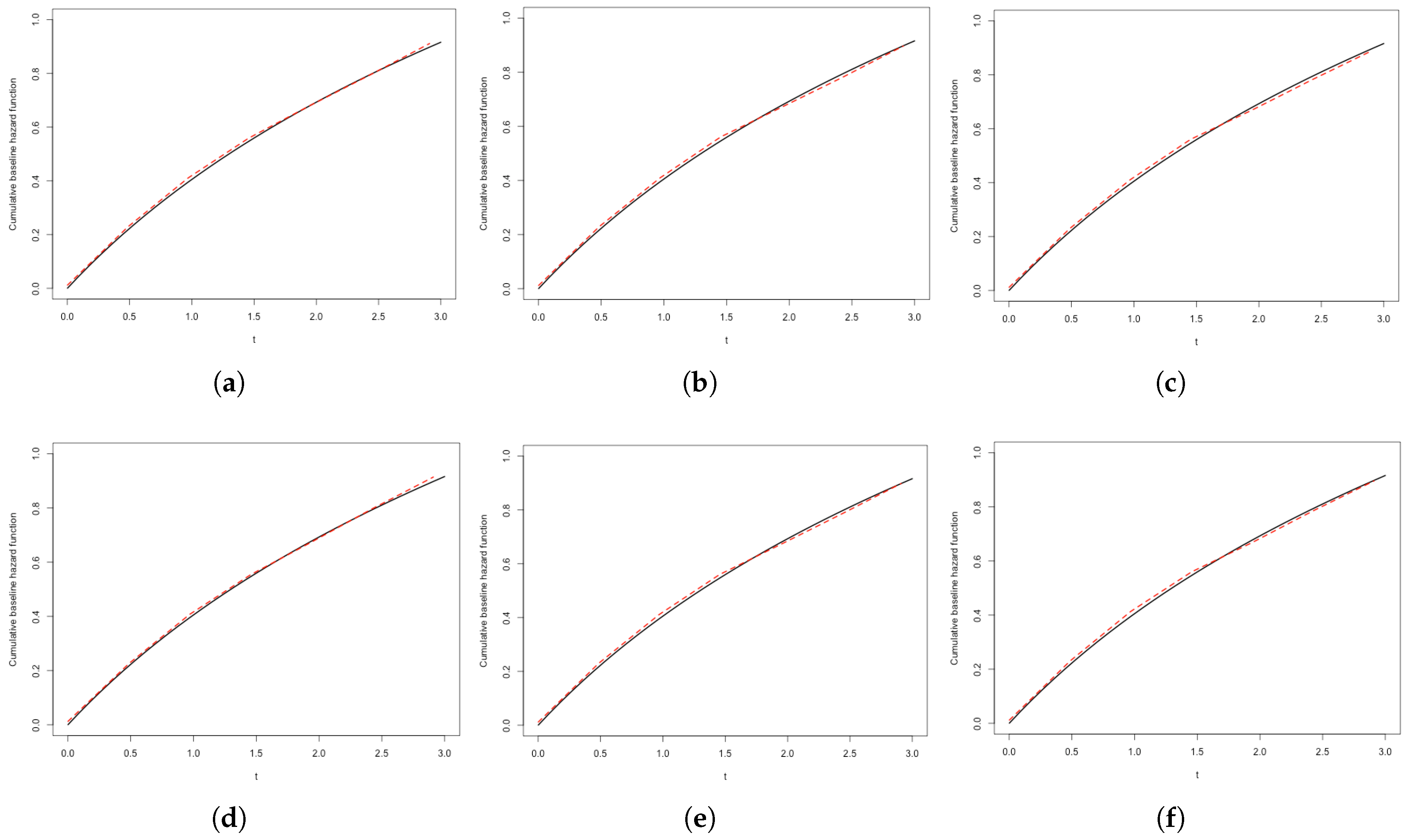
To further illustrate the computational performance of our approach,

Table 4. Number of iterations and average computation time per run under different parameter settings and sample sizes.

n	r	Iterations	Time (s)
200	0	922.44	1209.06
	$0.5$	1059.54	1559.32
	1	1138.89	1551.42
400	0	1124.32	4471.15
	$0.5$	1241.61	5663.02
	1	1282.80	4919.96

Note: Each row corresponds to a specific combination of transformation parameter r, with the associated sample size under $\zeta =0.75$. “Iterations” indicates the average number of iterations to convergence, and “Time (s)” is the average computation time based on 500 repetitions.

reports the average number of EM iterations and total runtime across various simulation settings. As expected, increases in sample size or the transformation parameter r are associated with higher computational demands, reflecting the greater complexity of model structure. Nevertheless, the proposed algorithm remains computationally feasible and exhibits stable convergence across all settings examined. We further visualize the estimated baseline function $\Lambda \left(t\right)$ alongside the true function in Figure 1, showing that the EM-based estimator effectively captures the underlying hazard dynamics. These findings collectively highlight the practical reliability and efficiency of our method in realistic interval-censored data contexts. While the simulation primarily focuses on moderate sample sizes and a fixed grid resolution for the change point, preliminary examinations suggest that the estimation results are relatively robust to alternative grid specifications.

6. Application

We applied the proposed EM-based transformation model to the PLCO (Prostate, Lung, Colorectal, and Ovarian) Cancer Screening Trial dataset to investigate whether a threshold effect exists in the relationship between age and colorectal cancer incidence, which has been widely accepted as a surrogate end point for disease progression [30]. The PLCO is a large-scale, multicenter randomized controlled trial initiated by the U.S. National Cancer Institute in 1993, designed to evaluate the effectiveness of various cancer screening strategies on cancer-specific mortality [31,32].

Our analysis focused on the incidence of colorectal cancer. The dataset consists of 60,598 participants, among whom approximately 98.7% of observations are right-censored, indicating a high degree of incomplete follow-up. To account for this and capture potential nonlinear covariate effects, we employed a semiparametric transformation model for survival outcomes. To explore the possible nonlinear influence of age, we modeled it as a threshold (or change point) variable. Specifically, we allowed the effect of age to change once it crosses an unknown threshold $\zeta$, which was estimated from the data using a grid search procedure embedded within the EM algorithm. The grid search was conducted over all unique observed age values in the dataset, ensuring that the threshold is data-driven and captures meaningful shifts in risk. This formulation introduces a binary indicator $\mathbb{I}\{\mathrm{Age}>\zeta \}$ into the linear predictor, allowing the model to detect and quantify a discrete change in risk associated with advancing age. Twelve covariates were included in the model: Race, Sex, Education, Employment, Cancer, Colorectal cancer, Diabetes, Stroke, Heart disease, Gallbladder disease, and Colorectal polyps. All variables were coded as binary indicators based on baseline questionnaire data. Initially, we also incorporated interaction terms between the thresholded age variable and all other covariates to test for potential effect modification. However, none of these interactions were statistically significant, and they were therefore omitted from the final model. To determine the most appropriate transformation structure, we varied the transformation parameter r over the interval $[0,1.5]$ in increments of 0.1 and evaluated model fit via the log-likelihood. The value $r=0$ corresponds to the Cox PH model, while $r=1$ corresponds to the PO model. We found that the log-likelihood increased monotonically with r, peaking at $r=1.5$. Accordingly, $r=1.5$ was selected as the best-fitting model, though results for $r=0$ and $r=1$ are also reported for comparison.

Table 5. Analysis results of the PLCO dataset, including the estimated covariate effect (Est), standard error estimate (SE), and p-value.

Covariate	r = 0			r = 1			r = 1.5
	Est	SE	p-Value	Est	SE	p-Value	Est	SE	p-Value
Race	0.509	0.161	0.002	0.517	0.166	0.002	0.521	0.167	0.002
Sex	0.319	0.086	<0.001	0.323	0.088	<0.001	0.326	0.088	<0.001
Education	−0.150	0.085	0.076	−0.151	0.086	0.079	−0.152	0.086	0.078
Employment	−0.080	0.100	0.422	−0.080	0.102	0.433	−0.079	0.102	0.434
Cancer	0.131	0.088	0.137	0.134	0.090	0.136	0.135	0.090	0.133
ColoCancer	0.180	0.125	0.152	0.184	0.129	0.154	0.185	0.129	0.151
Diabetes	0.118	0.149	0.431	0.118	0.153	0.441	0.118	0.153	0.442
Strokes	0.016	0.299	0.957	0.015	0.304	0.961	0.014	0.305	0.963
Heart	0.074	0.134	0.578	0.075	0.137	0.582	0.076	0.137	0.580
Gallblad	0.181	0.123	0.142	0.182	0.125	0.148	0.182	0.126	0.148
Colorectal Polyps	0.152	0.144	0.291	0.155	0.149	0.296	0.157	0.149	0.294
Age (>$\zeta$)	0.640	0.094	<0.001	0.649	0.093	<0.001	0.653	0.091	<0.001

Note: This table presents the covariate estimation results under three transformation models: $r=0$ corresponds to the proportional hazards model, $r=1$ to the proportional odds model, and $r=1.5$ represents the best-fitting model selected based on log-likelihood. “Est” denotes the estimated regression coefficient, “SE” is the standard error, and “p-value” assesses statistical significance. The age threshold $\zeta$ was re-estimated separately for each value of r, allowing for model-specific breakpoints.

presents the estimated regression coefficients, standard errors, and p-values under the three transformation specifications. The estimated age threshold was 62 years and was held fixed across all models. The age indicator $\mathbb{I}\{\mathrm{Age}>62\}$ was found to be highly significant in all models ($p<0.001$), suggesting a substantial increase in colorectal cancer risk beyond this threshold. Notably, age 62 aligns with current clinical guidelines: most major organizations—including the U.S. Preventive Services Task Force—recommend initiating colorectal cancer screening at age 45, and strongly endorse routine screening between ages 50 and 75. The identification of 62 as a data-driven risk threshold offers a potentially meaningful refinement for stratifying individuals by risk and tailoring screening strategies. This reinforces not only the clinical relevance of our result, but also the interpretability and practical utility of the threshold model in guiding age-based prevention policies. Under the best-fitting transformation model ($r=1.5$), the estimated coefficient for the thresholded age variable was 0.653 (SE = 0.091), corresponding to an approximate 1.92-fold increase in relative risk ($exp\left(0.653\right)\approx 1.92$) for individuals older than 62.

In addition to Age, both Race and Sex were consistently significant across all model specifications. Specifically, Race = 1 was associated with increased risk (coefficient = 0.521, $p=0.002$), as was Sex = 1 (coefficient = 0.326, $p<0.001$). These findings are consistent with existing epidemiological literature and may reflect differences in genetic predisposition, healthcare access, health behaviors, or screening participation across demographic groups. The variable Education = 1 showed a marginally protective effect ($p=0.078$), suggesting that higher educational attainment may be associated with reduced risk, potentially through improved health literacy or greater utilization of preventive services. Other covariates, including prior cancer history, diabetes, cardiovascular conditions, and colorectal polyps, were not statistically significant at conventional levels, although the direction and magnitude of their coefficients remained clinically plausible. Residual diagnostics revealed no substantial violations of model assumptions, supporting the adequacy of the transformation model in this context.

We found that $r=1.5$ consistently yielded the best model fit in terms of log-likelihood, indicating that the effect of covariates on the event time distribution may deviate from the assumptions of standard proportional hazards ($r=0$) or proportional odds ($r=1$) models. This suggests that a more flexible transformation function is better suited to capture the underlying risk structure, particularly in the presence of threshold effects or subtle nonlinearities. In our application, such flexibility is especially relevant given the observed change point effect and the potential complexity of age-related risk dynamics. To assess the robustness of our conclusions, we conducted sensitivity analyses by fitting models at adjacent transformation parameters (e.g., $r=0.3$, $r=0.7$, and $r=1.3$). The results showed that the estimated effects and significance patterns remained stable, supporting both the interpretability and reliability of our modeling framework. In summary, our findings highlight the practical utility of transformation models with threshold components for analyzing complex, censored survival data. The estimated age cutoff of 62 years not only aligns with known clinical trends but also offers a data-driven refinement that may inform individualized screening strategies for colorectal cancer. The combination of transformation modeling and EM-based estimation thus provides a flexible and effective approach for uncovering nonlinear and heterogeneous risk patterns in survival analysis.

7. Discussion

In this paper, we developed a semiparametric transformation model that incorporates an unknown change point under interval-censored data. By combining a grid search technique for estimating the change point with an EM algorithm to handle the nonparametric baseline hazard, we proposed an effective estimation procedure tailored to this challenging data structure. Simulation studies demonstrated that the proposed method performs well in terms of bias, standard error, and confidence interval coverage across a range of settings, including different sample sizes and change point locations. Moreover, our application to real-world colorectal cancer screening data highlighted the practical utility of the approach in identifying interpretable threshold effects that may inform clinical guidelines.

Despite the encouraging performance of our proposed method, several avenues remain for future enhancement. First, the estimation of the change point via grid search—though widely adopted and effective in our simulations—may involve non-negligible computational cost and raise concerns about sensitivity to grid resolution. Our preliminary results suggest that the estimator remains stable even near boundary values, but a more systematic evaluation of grid resolution and its impact on estimation accuracy and efficiency is warranted. Developing adaptive or data-driven grid strategies could further enhance scalability for large datasets. Additionally, while we adopted a standard fixed initialization for the EM algorithm, exploring multiple or data-adaptive starting points may improve convergence in more complex or high-dimensional settings. Incorporating acceleration techniques such as quasi-Newton updates or PX-EM [33,34,35] could also reduce computation time. From a theoretical perspective, it would be valuable to investigate the convergence rate of the estimated threshold $\widehat{\lambda }$. Formal results on parameter existence and convergence remain an important direction for future theoretical work. Finally, while our model emphasizes interpretability via threshold detection, a direct empirical comparison with flexible alternatives (e.g., spline-based methods) could further clarify trade-offs in terms of estimation efficiency, interpretability, and computational cost.

In addition, extending our framework to accommodate mixture cure models could be particularly useful in clinical contexts involving long-term survivors or latent subpopulations [36,37,38]. Incorporating change points in such settings may better capture heterogeneous risk patterns and improve understanding of treatment effects and disease dynamics. Finally, in the presence of high-dimensional covariates, model sparsity and multicollinearity may impact estimation stability. Incorporating regularization techniques such as Lasso or SCAD [39,40,41] could improve variable selection and estimation accuracy. Moreover, systematic sensitivity analyses—including those on initial values, grid density, and transformation function specification—would provide deeper insight into the robustness and practical utility of the method across diverse scenarios [42].

8. Conclusions

In summary, our study contributes to the methodological toolbox for survival analysis under interval-censoring by integrating flexible threshold modeling into the semiparametric transformation framework. This approach is both theoretically sound and practically applicable.

• A novel integration of change point detection within semiparametric transformation models tailored for interval-censored data.
• Use of an EM algorithm to efficiently estimate model parameters, including a nonparametric baseline hazard function.
• Simulation studies confirm robustness across a variety of settings, including different sample sizes and censoring scenarios.
• Real-world application to colorectal cancer screening data reveals interpretable age-related threshold effects.
• The model captures nonlinear risk structures that traditional spline or linear methods may overlook.
• Future directions include extending the approach to cure models and addressing sensitivity to grid resolution through adaptive search procedures.

As interval censoring remains common in biomedical research, continued methodological innovations in this area will enhance our ability to derive clinically meaningful and interpretable insights from complex time-to-event data.