A Biased–Randomized Iterated Local Search with Round-Robin for the Periodic Vehicle Routing Problem

Abstract

The periodic vehicle routing problem (PVRP) is a well-known challenge in real-life logistics, requiring the planning of vehicle routes over multiple days while enforcing visitation frequency constraints. Although numerous metaheuristic and exact methods have tackled various PVRP extensions, real-world settings call for additional features such as depot configurations, tight visitation frequency constraints, and heterogeneous fleets. In this paper, we present a two-phase biased–randomized algorithm that addresses these complexities. In the first phase, a round-robin assignment quickly generates feasible and promising solutions, ensuring each customer’s frequency requirement is met across the multi-day horizon. The second phase refines these assignments via an iterative search procedure, improving route efficiency and reducing total operational costs. Extensive experimentation on standard PVRP benchmarks shows that our approach is able to generate solutions of comparable quality to established state-of-the-art algorithms in relatively low computational times and stands out in many instances, making it a practical choice for real life multi-day vehicle routing applications.

1. Introduction

Vehicle routing problems (VRPs) are a frequent challenge in logistics and supply chain management, playing a key role in optimizing the delivery of goods and services while minimizing operational costs [1]. The fundamental objective in these problems is to determine efficient routes for a fleet of vehicles tasked with servicing a set of geographically dispersed customers. Given its complexity and real-world relevance, VRP has been extensively studied, leading to numerous extensions that account for additional constraints such as time windows, vehicle capacity, and dynamic demand fluctuations [2]. Among these extensions, the periodic vehicle routing problem (PVRP) introduces a multi-day planning horizon, where customers require service on multiple occasions throughout a defined period [3]. Unlike the classical VRP, which aims for a single optimal route configuration, PVRP requires the determination of how to distribute customer visits across different days while ensuring that specific frequency constraints are met. This additional temporal dimension increases problem complexity significantly, as solutions must balance route optimization with the constraints imposed by multi-day scheduling [4].

Over the years, a wide range of methodologies have been developed to tackle different PVRP variants, covering heuristics, metaheuristics, and exact approaches. Techniques such as tabu search, genetic algorithms, and column generation-based heuristics have proven effective in various instances, particularly in small- to medium-sized problems. However, many real-world applications present additional challenges that existing methods find difficult to address efficiently. Despite the progress made in PVRP research, solving large-scale instances with these added constraints remains a significant challenge. Many existing algorithms focus on static or homogeneous fleet settings, limiting their applicability to real-world logistics problems that require adaptability and scalability. Moreover, methods that produce high-quality solutions often do so at the expense of increased computational time, making them impractical for dynamic logistics operations, where quick decision making is essential.

To address these limitations, this paper proposes a two-phase approach designed to efficiently tackle the PVRP. The first phase of our method employs a biased–randomized round-robin assignment strategy to generate an initial feasible solution, ensuring that each customer receives service according to the required frequency while distributing the workload across vehicles and depots. This initial phase provides a fast, structured allocation of resources, establishing a baseline solution that respects frequency constraints without requiring extensive computational effort. Building upon this initial solution, the second phase refines the routing plan through an iterative local search procedure, incorporating neighborhood-based optimization techniques that systematically improve route efficiency and reduce operational costs. By using this two-stage structure, the proposed method balances computational efficiency with high-quality solution generation, making it suitable for practical deployment in complex logistics environments. A key advantage of this approach is its adaptability to real-world constraints, allowing for extensions that accommodate operational requirements such as time windows, driver consistency, and stochastic demand variations. While many heuristic and metaheuristic approaches focus exclusively on achieving the best possible solution within a static environment, the method presented in this work is designed with flexibility in mind, making it well suited for dynamic and large-scale routing applications.

The computational evaluation of our approach demonstrates its effectiveness in solving benchmark instances of the PVRP. Extensive experiments show that our algorithm achieves solutions of comparable or superior quality to some existing state-of-the-art methods while maintaining manageable computational times. In particular, results indicate that our method performs robustly across different instance sizes, handling both small-scale problems where solutions converge quickly and larger, more complex instances where solution quality is highly dependent on refinement strategies. The ability to scale efficiently while maintaining solution quality positions our approach as a promising alternative for real-life logistics services. The following sections are organized as follows. Section 2 reviews the most relevant literature on the PVRP and its extensions, emphasizing existing solution methodologies and their limitations. Section 3 provides a formal mathematical formulation of the problem, specifying its objectives and constraints. Section 4 details a two-phase heuristic, outlining the rationale for its design and its main algorithmic components. Section 5 and Section 6 describe the experimental setup and analyze the results obtained on benchmark instances, contrasting the proposed approach with state-of-the-art methods. Aditionally we present a simple way to extend our algorithm to stochastic environments. Finally, Section 7 presents concluding remarks and highlights avenues for future research as well as the practical applications of the method.

2. Related Work

The PVRP is a well-known problem in the literature. In [3], the authors review the life of a problem that was first defined by [5] in the context of waste collection. However, this problem can be applied in many different areas, such as healthcare [6,7], maintenance [8], and supply chains [9,10]. To solve the PVRP, various methodologies have been studied, both through exact methods and metaheuristics. In terms of exact methods, it is important to highlight the work of [11], which aims to solve the problem exactly by applying certain relaxations to the original problem to find lower bounds, using its dual nature to generate routes with the objective of obtaining the optimal solution. Another exact approach to consider is the work of [12], in which an exact branch-and-cut algorithm is proposed to solve an extension of the problem with driver consistency. Additionally, there are methodologies based on column generation, as in the work of [13], which focuses on grouping the nodes into clusters that can be traversed by the vehicles. Column generation thus relies on progressively considering more and more of these clusters in a linear optimization problem.

Regarding metaheuristic algorithms, several approaches have been explored. One of the first contributions to metaheuristic approaches is the work of [14] (CGL), where a tabu search [15] is defined to avoid falling into local minima. Another approach that achieved good results is scatter search [16] in the work of [17] (ALP), where a reference set is generated with a heuristic solution generation and some local search methods such as CROSS [18] and Or’s interchanges [19]. As is common in routing problems, a solution based on variable neighborhood search (VNS) has also been explored, as seen in the work of [20] (HDH), where up to 15 neighborhood structures, changing patterns, and route nodes are proposed. Despite being local search processes similar to those defined in this work, it can be observed that performance improved even when compared to the longest executions, where they applied up to ${10}^9$ iterations.

The most recent works that have provided the best results and with which we will compare in this article are SC-Heur [21] and HGADC [22]. Using column generation, in SC-Heur, a problem is defined based on set covering followed by iterated local search (ILS). On the other hand, HGADC aims to represent the solution with two distinct chromosomes, where the first refers to the selected pattern for collections and the other directly to the route. An educational phase is also added to improve solutions through various local search methods, such as unified tabu search (UTS) and random variable neighborhood search (RVNS). Hybrid genetic algorithms are widely use with very promising results in vehicle routing problems [23] or other fields like road networks [24].

Finally, it is worth highlighting a recent work in which the authors show that over a longer planning horizon, it is possible to maintain workload equity without increasing routing costs. Also notable are the works of [25,26], which employ techniques similar in spirit to those presented in this study, i.e., the diverse generation of solutions to search for the best one. In their case, these techniques are applied to the multi-depot vehicle routing problem (MDVRP) and the multi-period vehicle routing problem (MPVRP).

3. A Mathematical Model for the Periodic Vehicle Routing Problem

The PVRP was first introduced in the waste collection study by [5]. However, their work did not present a mathematical formulation of the problem. It was [27] who later provided an integer programming formulation for a version of the PVRP. Since then, three modeling lines have dominated the literature. Vehicle-indexed flow models with Miller–Tucker–Zemlin (MTZ) subtour elimination constraints offer compact mixed-integer programs and remain effective for medium-sized instances [28]. Load or commodity flow formulations aggregate vehicle load variables and yield stronger linear relaxations at the price of additional variables [29]. Cut-based or set-partitioning formulations serve as the foundation of modern branch-and-cut and branch-and-price algorithms and easily incorporate further constraints such as driver consistency [12]. A recent head-to-head comparison of these families [28] shows that the compact MTZ model continues to be competitive for the plain PVRP, that is, the variant without time windows or other extensions. The following formulation is defined over a directed graph using arcs. In this work, we focus on an undirected setting based on edges, but the structure and logic of the formulation remain applicable.

Let $G=(N,A)$ be a complete directed graph with depot 0 and customer set $N_c=N\setminus \left\{0\right\}$. The planning horizon is $T=\{1,\dots ,\tau \}$. Each vehicle has capacity Q, and the maximum number of vehicles available per day is $\kappa$. For every customer $i\in N_c$, a demand $d_i>0$ is specified together with an admissible set of visit patterns $P_i$. The decision variables are $x_{ijt}\in \{0,1\}$, indicating whether arc $(i,j)$ is traveled on day t. $y_{it}\in \{0,1\}$ indicates whether customer i is served on day t. $s_{ip}\in \{0,1\}$ selects pattern $p\in P_i$, and continuous load variables $u_{it}$, giving the vehicle load at customer i on day t. The model can be expressed as follows:

$$\begin{array}{cc}\hfill min& \sum _{(i,j)\in A}\sum _{t\in T}{c}_{ij}{x}_{ijt}\hfill \end{array}$$

(1)

$$\begin{array}{cccc}\hfill \mathrm{s}.\mathrm{t}.& \sum _{p\in P_i}{s}_{ip}=1\hfill & \hfill & \forall i\in N_c\hfill \end{array}$$

(2)

$$\begin{array}{cccc}\hfill & \sum _{p\in P_i:t\in p}{s}_{ip}=y_{it}\hfill & \hfill & \forall i\in N_c,\forall t\in T\hfill \end{array}$$

(3)

$$\begin{array}{cccc}\hfill & x_{ijt}\le {\displaystyle \frac{y_{it}+y_{jt}}{2}}\hfill & \hfill & \forall i,j\in N_c,\forall t\in T\hfill \end{array}$$

(4)

$$\begin{array}{cccc}\hfill & \sum _{j\in N_c}{x}_{0jt}\le \kappa \hfill & \hfill & \forall t\in T\hfill \end{array}$$

(5)

$$\begin{array}{cccc}\hfill & \sum _{j\in N\setminus \left\{i\right\}}{x}_{ijt}=y_{it}\hfill & \hfill & \forall i\in N_c,\forall t\in T\hfill \end{array}$$

(6)

$$\begin{array}{cccc}\hfill & \sum _{j\in N\setminus \left\{i\right\}}{x}_{jit}=y_{it}\hfill & \hfill & \forall i\in N_c,\forall t\in T\hfill \end{array}$$

(7)

$$\begin{array}{cccc}\hfill & u_{jt}\le u_{it}-d_i{y}_{it}+Q\left(1-x_{ijt}\right)\hfill & \hfill & \forall i,j\in N_c,\forall t\in T\hfill \end{array}$$

(8)

$$\begin{array}{cccc}\hfill & d_i\le u_{it}\le Q\hfill & \hfill & \forall i\in N_c,\forall t\in T\hfill \end{array}$$

(9)

$$\begin{array}{cccc}\hfill & x_{ijt}\in \{0,1\}\hfill & \hfill & \forall (i,j)\in A,\forall t\in T\hfill \end{array}$$

(10)

$$\begin{array}{cccc}\hfill & s_{ip}\in \{0,1\}\hfill & \hfill & \forall i\in N_c,\forall p\in P_i\hfill \end{array}$$

(11)

$$\begin{array}{cccc}\hfill & y_{it}\in \{0,1\}\hfill & \hfill & \forall i\in N_c,\forall t\in T.\hfill \end{array}$$

(12)

Constraints (2) force every customer to choose exactly one admissible visit pattern. Constraints (3) activate the daily visit indicator whenever the chosen pattern contains the corresponding day. Constraints (4) allow an arc to be used on day t only if both of its endpoint customers are scheduled that day. Constraints (5) limit the number of vehicles that can leave the depot per period. Constraints (6) and (7) impose flow conservation by requiring exactly one outgoing and one incoming arc for each visited customer on each day. Constraints (8) represent the Miller–Tucker–Zemlin inequality that propagates the remaining vehicle load along the tour and prevents subtours. Constraints (9) keep the load between the current customer demand and the vehicle capacity. Binary restrictions are stated in Constraints (10)–(12).

4. Solution Approaches for the Periodic Vehicle Routing Problem

In this section, we propose a two-phase methodology to solve the PVRP. The first phase focuses on building maps (or preliminary solutions) by assigning each customer to specific days and vehicles in a fast robust manner, following a round-robin tournament process [30], whilst also introducing a biased randomization process [31] to randomize the generation in order to generate diverse initial solutions and a multi-start algorithm. The second phase then refines these maps via an ILS procedure [32], incorporating neighborhood-based improvements and strategic perturbations.

4.1. Phase 1: Map Generation

In the first phase of the algorithm, the goal is to generate ‘maps’ with high-quality feasible solutions. To achieve this, the solution is built by assigning nodes to vehicles using the round-robin method, that is, the vehicles take turns selecting the nodes to be assigned to them. To further diversify the initial solution generation, the chosen element (vehicle or node) is selected through a biased GRASP procedure [31]. This is a variant of the GRASP metaheuristic algorithm [33], where the elements to be selected are ordered in a list using a greedy function, such as the distance between a node and the last one selected in a routing problem. Once the list is generated, an element is randomly selected. In the original GRASP algorithm, the element is randomly chosen from a sub-list filtered by a parameter $\alpha$. 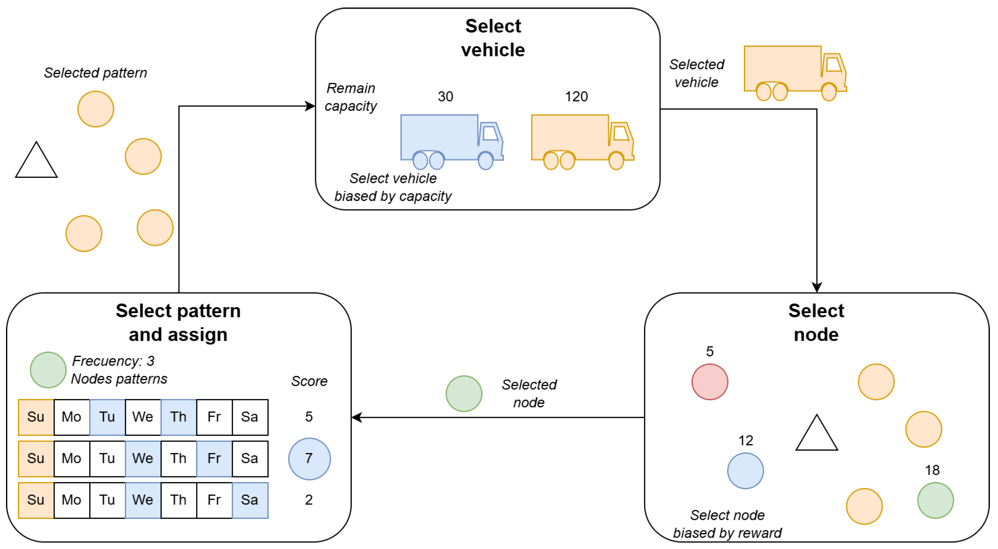However, in the biased randomization variant, the element is randomly selected following a right-skewed distribution, where the first elements (those with better values in the greedy function) are more likely to be chosen than the last ones. In this generation process, there are three sequenced phases that are repeated until a feasible solution is obtained: the selection of the vehicle, the selection of the node, and the selection of the pattern.

For vehicle selection during the round-robin process, the vehicles from all periods are sorted based on their remaining capacity, either in ascending or descending order. Sorting them by the highest remaining capacity leads to more balanced solutions, where capacity usage is evenly distributed among all vehicles. On the other hand, sorting them by the lowest remaining capacity results in filling the vehicle capacity as soon as possible, leading to solutions that aim to minimize the number of vehicles used. Depending on the instance type, one policy may be better than the other. To introduce diversity in the map’s generation, this selection follows a biased randomization procedure, with geometric distribution of parameter ${\beta }_1$ and the greedy function throughout the remaining capacity, as defined before. Given a selected vehicle, the next step is to choose a node to add to its route. The chosen node should contribute to create a good route for that vehicle and must not exceed its capacity. Therefore, candidate nodes for the route are ranked based on a score. In this algorithm, they are sorted according to the k-nearest nodes criterion, meaning the score assigned to a node is determined by the average distance between the node and the k-nearest nodes within that route. To further diversify the initial solution generation, the chosen node is selected through a geometric distribution of parameter ${\beta }_2$, where the greedy function is the k-nearest nodes criterion.

Once the node is chosen, its frequency is considered to select the pattern. If the frequency $f=1$, the node is simply added to the route, since the only possible pattern is that of frequency 1 that involves it. However, if $f>1$, then we must find $f-1$ vehicles from different periods to also ‘accommodate’ this node. We search among all possible patterns for that frequency and explore the best vehicles within each combination to insert the node, selecting the pattern with the best sum of scores. If no feasible combination of periods and vehicles is found, a different node must be selected. Finally, notice that this process assigns only nodes to vehicles and assigns patterns, but the sequence of the route is not determined. In order to generate a good sequence, a basic nearest-node heuristic is performed for each vehicle of each day. In the next phase, all the local searchesdefined will improve the sequence of these routes. A diagram of the entire map generation process can be found in Figure 1.

Algorithm 1 details the pseudo-code for this process. Here, the vehicle states track how much remaining capacity is available each day, while the dictionary of scores (or node_dict_score) is used to rank potential candidates with a biased selection (e.g., nearest in distance, marginal saving, etc.). If at any point the algorithm cannot accommodate a given subset of customers, the map generation fails and the process is started again.

Algorithm 1 Map generation (Phase 1)

1: Initialize: $\mathit{vehicleStates}$ with each $(\mathrm{day},\mathrm{vehicle})$ having full capacity 2: $\mathit{assignedCustomers}\leftarrow 0$ 3: while $(\mathit{assignedCustomers}<|\mathcal{N}|-1)$ do 4:     $(d_1,v_1)\leftarrow \mathit{biasSelectPair}\left(\mathit{vehicleStates}\right)$                      ▹ Choose day-vehicle with capacity 5:     $\mathit{selected}\leftarrow \mathit{biasSelectCustomer}(d_1,v_1)$                                                     ▹ Choose customer 6:     $((d_2,\dots ,d_f),(v_2,\dots ,v_f))\leftarrow \mathit{chooseBestPattern}\left(\mathit{selected}\right)$                            ▹ Choose pattern 7:     $\mathit{assignCustomer}(\mathit{selected},(d_1,\dots ,d_f,v_1,\dots ,v_f))$ 8:     $\mathit{assignedCustomers}\leftarrow \mathit{assignedCustomers}+1$ 9:     Update(vehicleStates) 10: end while 11: return $\mathit{Map}$

At the end of Phase 1, each customer is assigned to specific routes across multiple days. Although these assignments might not be globally optimal, they typically ensure full coverage (i.e., all frequencies are respected). The next phase further refines these initial solutions to minimize total distance and mitigate potential constraint violations.

4.2. Phase 2: Refinement via ILS

Although the construction strategy described above rapidly assigns customers to days and vehicles, its primary aim is to achieve a feasible solution rather than an optimized one. To further reduce total travel distance, we employ an ILS method that systematically refines the output in which all frequency requirements are satisfied. The ILS then performs repeated cycles of local search and perturbation, allowing it to navigate the solution space. The local search focuses on neighborhood moves within a given day, trying to obtain optimized solutions day by day. For this, we consider three local search operators, detailed as follows.

• Intra-route 2-node exchange: This local search improves existing routes through re-sequencing. Given a route, two nodes i and j are selected and swapped, analyzing the improvement in the objective function.
• Inter-route 2-node exchange: For instances with more than one route per day, it is necessary to explore the exchange of nodes between routes. Given two routes on the same day, the algorithm explores swapping node i from the first route with node j from the second.
• Change route: Since this is a capacity-constrained problem, some routes may have more nodes than others. Therefore, it is necessary to explore the reassignment of a node to a different route on the same day.

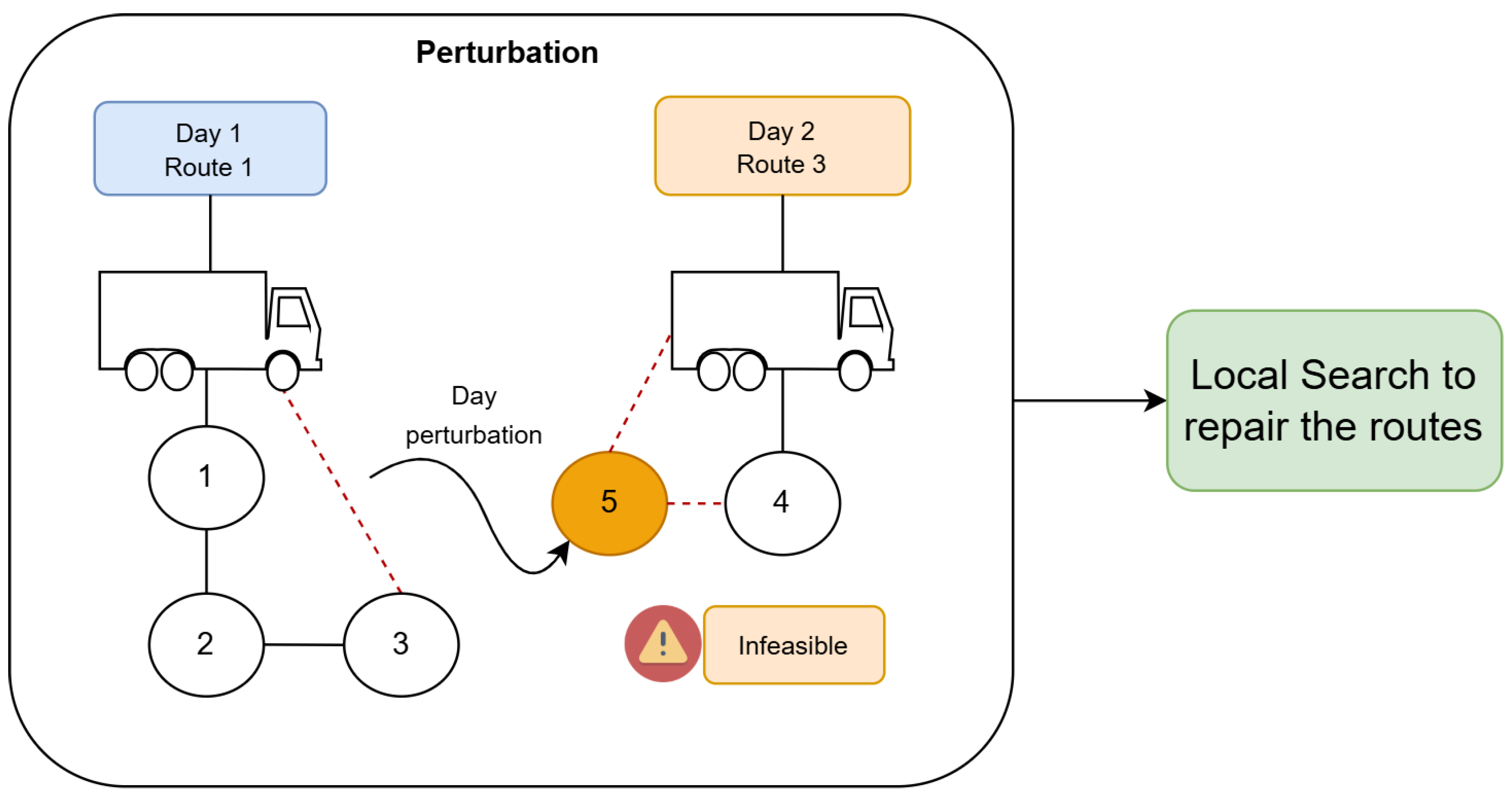
Because no direct exchanges across different days occur in these local search steps, a perturbation mechanism is required to move customers between days if a different assignment might obtain an overall improvement. Additionally, to avoid becoming stuck in local minima on a day-to-day basis, we also introduce a perturbation mechanism for routes within the same day. Thus, in our implementation, a random subset of customers is periodically shaken from their current day-vehicle routes and reassigned to random alternative days or vehicles, following one of the following perturbation mechanisms:

• Day perturbation: A set of n nodes is randomly selected, and the pattern of each node is randomly reassigned among all possible pattern options, assigning each node to the vehicle with the greatest available capacity. In this way, new node–day configurations are explored (Figure 2).
• Route perturbation: A set of n nodes are randomly selected and reassigned to a random different route on the same day at random. This allows the exploration of new routes within the same day and helps avoid becoming stuck in local minima.

Notice that this procedure can lead to short-term capacity violations or over-coverage of certain days, but those partial infeasibilities are penalized in the objective function. This penalty-based approach improves exploration capability, enabling the system to discover new day–vehicle configurations that would remain unreachable if the local search were restricted to day-level moves alone.

We integrate a simulated annealing acceptance criterion into the ILS loop so that a newly generated solution can replace the current solution not only when its cost is lower, but also with a small probability, even if it is temporarily worse. This controlled tolerance for cost increases allows the search a chance to escape pronounced local minima and explore more varied regions of the solution space. By combining these mechanisms, namely, fast local search on each day, cross-day perturbations, and probabilistic acceptance of non improving moves, the day vehicle assignments built in Phase 1 are enhanced while ensuring that the overall method remains computationally efficient.

Algorithm 2 summarizes the ILS refinement procedure. The approach begins by constructing an initial feasible solution from the Phase 1 map and repeatedly applies local search and perturbation until a maximum number of iterations is reached. The result is a refined multi-day routing plan that respects customer frequencies, capacities, and day–vehicle allocations, with a significantly lower overall travel cost than the initial assignment.

Algorithm 2 Refinement via iterated local search (Phase 2)

1: $\mathit{bestSol}\leftarrow \mathit{buildGreedyRoutes}\left(\mathit{Map}\right)$ 2: $\mathit{currentSol}\leftarrow \mathit{bestSol};T\leftarrow T_{\mathrm{init}};\mathit{noImprovement}\leftarrow 0$ 3: for $\mathit{iter}\in \{1,\dots ,\mathit{maxIter}\}$ do 4:     $\mathit{newSol}\leftarrow \mathit{Perturb}\left(\mathit{currentSol}\right)$ 5:     $\mathit{newSol}\leftarrow \mathit{LocalSearch}\left(\mathit{newSol}\right)$ 6:     $\Delta \leftarrow \mathit{newSol}.\mathit{cost}-\mathit{currentSol}.\mathit{cost}$ 7:     if ($\Delta <0$) or ($\mathit{rand}<e^{-\Delta /T}$) then 8:         $\mathit{currentSol}\leftarrow \mathit{newSol}$ 9:         if $\mathit{currentSol}.\mathit{cost}<\mathit{bestSol}.\mathit{cost}$ then 10:            $\mathit{bestSol}\leftarrow \mathit{currentSol};\mathit{noImprovement}\leftarrow 0$ 11:         else 12:            $\mathit{noImprovement}\leftarrow \mathit{noImprovement}+1$ 13:         end if 14:     end if 15:     $Update\left(T\right)$ 16: end for 17: return $\mathit{bestSol}$

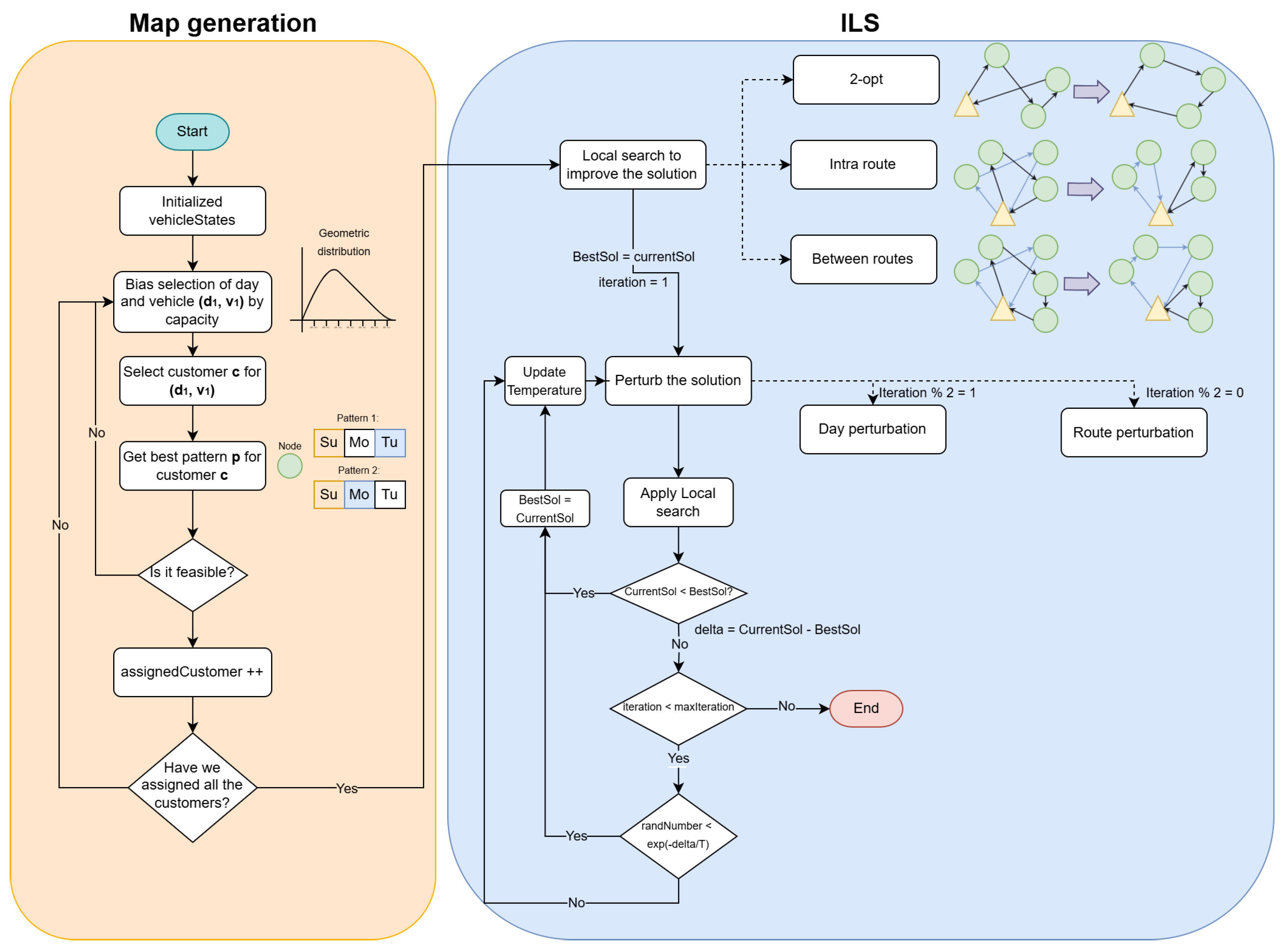
Figure 3 presents a clear visual summary of the methodological steps involved in the two-phase solution approach. This integrated diagram connects the map generation and refinement processes into a single, coherent representation. It explicitly shows how the initial map, generated through biased–randomized selection, naturally progresses into iterative refinement via local search and perturbation mechanisms. By combining these aspects, the flowchart serves as an accessible reference, facilitating both comprehension and practical implementation of the proposed algorithmic framework.

5. Numerical Experiments

This section outlines the computational experiments we conducted to evaluate the efficiency and performance of the previously discussed algorithms.

All algorithms were implemented using Julia version $1.11$ and executed on the Google Cloud Platform [34] equipped with an AMD Milan CPU, c2d-standard-4 machine type with 4 vCPUs, 16 GB of RAM, and a Debian 11 operating system. For experimental purposes, we used the benchmark set proposed by [14], as it is widely used in the literature to assess the performance of algorithms designed to solve the classical version of PVRP.

For the smaller benchmark instances (p01 to p26), we allowed a total run time of one hour and imposed a cap of ${10}^6$ iterations in our ILS. Meanwhile, for the larger and more complex instances (p27 to p32), we increased the time limit to two hours and allowed up to $3\times {10}^6$ iterations. These limits were selected to balance the thorough exploration of solution neighborhoods against practical runtime considerations, given the NP-hard nature of the problem.

For the smaller benchmark instances (p01 to p26), we allowed a total run time of one hour and imposed a cap of ${10}^6$ iterations in our ILS. Meanwhile, for the larger and more complex instances (p27 to p32), we increased the time limit to two hours and allowed up to $3\times {10}^6$ iterations. The time selected for this experiment was set based on the last article, which brought the new best known solutions to the state-of-the-art level [21]. These limits were selected to balance the thorough exploration of solution neighborhoods against practical runtime considerations, given the NP-hard nature of the problem. It should be noted that these run times represent maximum limits. The best solution is not necessarily obtained precisely at the end of the algorithm’s time limit.

5.1. Selection of Parameter Values

In Section 4, the methodology of the algorithm and its two components are detailed. Several hyper-parameters are required and need to be tuned. To select appropriate values, we use self-tuning techniques during map generation, allowing room to explore different parameter values and generate more diverse initial solutions. For the improvement procedure in the ILS, we rely on results from previous studies to adjust the parameters. In the first phase, the biased round-robin depends on the parameter ${\beta }_1$, which defines the geometric distribution that controls the degree of randomness used to select a vehicle, and ${\beta }_2$, which similarly controls the randomness used to select a node. These parameters are tuned using the procedure described in Martin et al. [35]. In this approach, the authors utilize a triangular probability distribution over the interval $[0,1]$, with its mode positioned at the parameter value ${\beta }^{\prime }$, the value that demonstrated the best performance in previous runs. Initially, ${\beta }^{\prime }$ is assigned a value of $0.5$. In later iterations, parameter values are drawn from this distribution, encouraging selections near ${\beta }^{\prime }$ while still allowing for diversity across runs. This approach enables customized self-tuning for each instance, thus avoiding parameter overfitting.

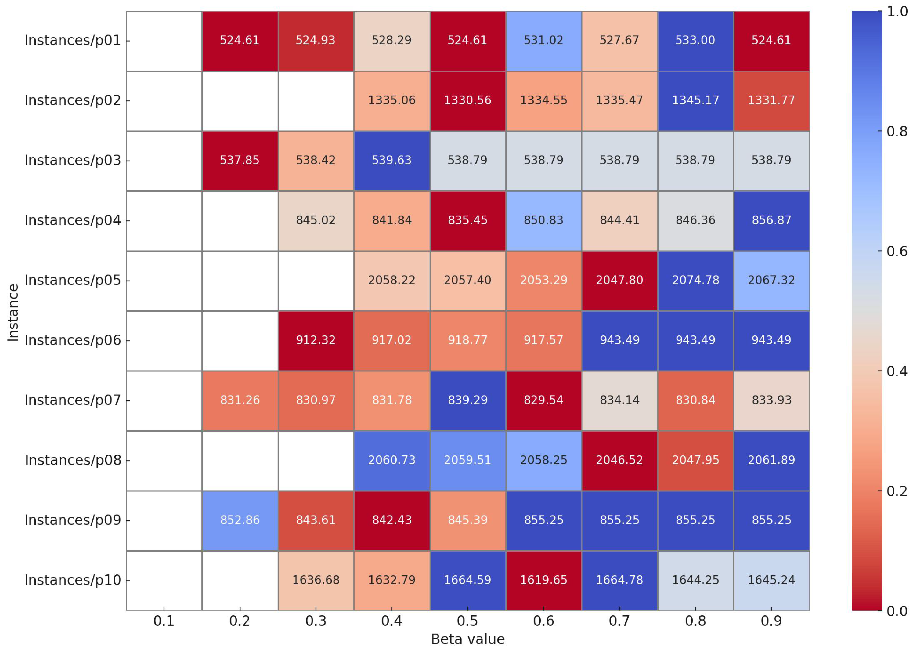
To better understand the influence of the node selection parameter on our biased–randomized round-robin strategy, we performed a dedicated sensitivity analysis. We tested values of ${\beta }_1$ ranging from 0.1 to 0.9 and measured the corresponding objective values on the first ten benchmark instances, using a time budget of 60 s per run. The results are shown in Figure 4, where each cell represents the objective function for a given instance and a specific ${\beta }_1$ value. Cells without a numerical value correspond to infeasible solutions, where no valid result was found within the time limit.

The heat map reveals that performance varies across instances, with some benefiting from more exploratory configurations and others from more deterministic ones (where red indicates better objective function values and blue denotes worse ones). Although the optimal setting differs from case to case, no single value consistently outperforms the rest. To maintain generality and avoid tuning the algorithm too closely to the selected problems, we fix ${\beta }_1$ at 0.5 for all comparative runs.

On the other hand, there is the tuning of the parameters for the ILS procedure, where the value used to accept a change in the solution through the simulated annealing procedure is given by $e^{-(o{f}_{new}-o{f}_{current})/T}$. To choose a suitable initial temperature, we relied on the study presented in [20], where appropriate temperature magnitudes are described. Based on this, we set $T=7$ for small instances (p1–p26) and $T=100$ for large instances (p27–p32). The temperature decreases linearly every 1000 iterations until it reaches 0 in the final iteration of the ILS. As for the perturbation of routes and periods, we opted to randomly change between 0 and 3 nodes in both cases, aiming to make controlled changes as recommended in the same work.

5.2. Stochastic Extension of the PVRP

Real-world distribution systems rarely operate under fully deterministic conditions. Key elements such as travel times, customer demands, and service durations are better modeled as stochastic variables, as they are naturally subject to uncertainty. Ignoring this variability often produces fragile routing plans whose expected cost is seriously underestimated. Consequently, modern solution methods must incorporate stochastic information from the outset rather than adding it as an afterthought.

One practical way to achieve this is through a simheuristic framework [36], where a metaheuristic explores the deterministic search space, and a Monte Carlo simulation module is executed to estimate the performance of the most promising candidates under uncertainty. Because simulation is applied selectively, the additional computational effort remains moderate while the algorithm obtains information about risk and variability. This approach has been widely applied to solve stochastic variants of combinatorial optimization problems, particularly in logistics and transportation domains.

Other metaheuristic frameworks, such as genetic algorithms, maintain a population with many individuals in each generation. Evaluating them under uncertainty requires as many independent simulations as there are solutions, which quickly turns simulation into the main contributor to total runtime. Hybrid approaches that combine heuristics with exact methods face similar difficulties. Incorporating stochastic elements into a mixed-integer formulation typically increases the size of the model or forces the use of basic deterministic approximations.

The proposed GR-BRILS algorithm generates a single complete routing plan at each iteration. This design keeps the simulation effort limited, since only one solution needs to be evaluated at a time. As a result, the algorithm remains efficient, even when operating under uncertain conditions such as stochastic demands or travel times.

To quantify a solution’s resilience under uncertainty, we incorporate the concept of reliability (r), which quantifies how often a solution remains feasible under stochastic conditions. In our experiments, reliability is computed as $1-{\displaystyle \frac{\mathrm{failures}}{\mathrm{number}\mathrm{of}\mathrm{simulations}}}$, where a failure corresponds to a simulated scenario in which the routing plan violates problem constraints. This metric offers a practical measure of robustness and highlights how solutions with low reliability may require costly adjustments, ultimately reducing their real-world effectiveness.

To assess the effectiveness of simheuristic methods in this context, we compare GR-BRILS with a static baseline on benchmark instances in which customer demand is modelled as a lognormally distributed random variable—a common choice for representing positive, right-skewed demand in logistics—using the original deterministic demand as the mean and a fixed variance ($\sigma$) of 0.5. Both algorithms are executed for 5 min per instance, and their results are reported in

Table 1. Reliability comparison between GR-BRILS and SimGR-BRILS for $\sigma =0.5$.

Instance	GR-BRILS		SimGR-BRILS		r-Gap
	FO	$\mathit{r}$	FO	$\mathit{r}$
p01	527.70	0.22	536.04	0.46	52.17%
p02	1334.18	0.54	1335.06	0.84	35.71%
p03	564.69	0.26	594.60	0.90	71.11%
p04	858.13	0.04	868.31	0.45	91.11%
p05	2085.12	0.16	2100.41	0.19	15.79%
p06	977.32	0.36	981.99	0.62	41.94%
p07	838.16	0.50	840.56	0.91	45.05%
p08	2059.64	0.09	2096.65	0.33	72.73%
p09	885.78	0.54	928.29	1.00	46.00%
p10	1671.07	0.10	1696.80	0.70	85.71%

. The data show that SimGR-BRILS captures the impact of stochastic variability more effectively than the static approach, which performs simulation only after constructing the final solution. Although the static version tends to achieve better objective values under deterministic assumptions, it is often sensitive to small demand fluctuations, which may result in infeasibility. By integrating simulation during the search, SimGR-BRILS is able to consider uncertainty dynamically, delivering solutions that are more robust and practically applicable, even at the cost of a marginal increase in expected objective value.

6. Analysis of Results

This section presents an evaluation of the computational results obtained from the benchmark instances used to compare the six algorithms: CGL, ALP, HDH, HGADC, SC-Heur, and GR-BRILS. This algorithms are referenced in Section 2. For CGL and ALP, only one seed is used in the original work. For HDH, only the average across 10 seeds is used, and we selected the ${10}^7$ iteration performances for this algorithm, as the works of HGADC and SC-Heur did to compare its performance to HDH. The primary objective is to assess the quality of the solutions generated by each method and determine their effectiveness across different problem sizes.

Table 2. Average objective function values.

Instance	CGL	ALP	HDH	HGADC	SC-Heur	GR-BRILS
p01	524.61	531.02	524.61	524.61	524.61	524.61
p02	1330.09	1324.74	1332.01	1322.87	1326.16	1323.14
p03	524.61	537.37	528.97	524.61	524.61	527.06
p04	837.93	845.97	847.48	836.59	837.04	836.07
p05	2061.36	2043.75	2059.74	2033.72	2048.29	2041.04
p06	840.3	840.1	884.69	842.48	841.96	907.36
p07	829.37	829.65	829.92	827.02	834.14	830.22
p08	2054.9	2052.21	2058.36	2022.85	2042.02	2045.25
p09	829.45	829.65	834.92	826.94	847.03	834.35
p10	1629.96	1621.21	1629.76	1605.22	1664.90	1625.26
p11	817.56	782.17	791.18	790.77	775.84	795.16
p12	1239.58	1230.95	1258.46	1195.29	1228.14	1262.92
p13	3602.76	-	3835.9	3599.86	3549.30	3833.46
p14	954.81	954.81	954.81	954.81	954.81	954.81
p15	1862.63	1862.63	1862.63	1862.63	1862.63	1862.63
p16	2875.24	2875.24	2875.24	2875.24	2875.24	2875.24
p17	1597.75	1597.75	1601.75	1597.75	1597.75	1597.75
p18	3159.22	3157	3147.91	3131.09	3149.09	3149.46
p19	4902.64	4846.49	4851.41	4834.50	4839.87	4846.49
p20	8367.40	8412.02	8367.40	8367.40	8367.40	8512.00
p21	2184.04	2173.58	2180.33	2170.61	2170.61	2183.02
p22	4307.19	4330.59	4218.46	4194.23	4232.50	4270.42
p23	6620.5	6813.45	6644.93	6434.10	6573.33	6637.09
p24	3704.11	3702.02	3704.6	3687.46	3687.46	3689.11
p25	3781.38	3781.38	3781.38	3777.15	3777.15	3779.40
p26	3795.32	3795.33	3795.32	3795.32	3795.32	3795.32
Av. gap % Small	0.98%	0.95%	1.36%	0.14%	0.61%	1.42%
p27	23,017.54	22,561.33	22,153.31	21,885.70	21,963.23	21,959.18
p28	22,569.4	22,562.44	22,418.52	22,272.60	22,271.91	22,328.25
p29	24,012.92	23,752.15	22,864.23	22,564.05	22,564.80	22,612.83
p30	77,179.33	76,793.99	75,579.23	74,534.38	75,193.09	74,368.02
p31	79,382.35	77,944.79	77,459.14	76,686.65	76,496.67	76,555.01
p32	80,908.95	81,055.52	79,487.97	78,168.82	78,065.24	77,941.30
Av. gap % Large	4.05%	3.13%	1.35%	0.13%	0.27%	0.15%
Av. gap % All	1.56%	1.33%	1.36%	0.14%	0.54%	1.18%

and

Table 3. Minimum objective function values.

Instance	CGL	ALP	HDH	HGADC	SC-Heur	GR-BRILS
p01	524.61	531.02	524.61	524.61	524.61	524.61
p02	1330.09	1324.74	1332.01	1322.87	1322.87	1322.87
p03	524.61	537.37	528.97	524.61	524.61	524.61
p04	837.93	845.97	847.48	835.26	853.26	835.26
p05	2061.36	2043.75	2059.74	2024.96	2024.31	2038.4
p06	840.3	840.1	884.69	835.26	835.41	904.34
p07	829.37	829.65	829.92	826.14	829.63	829.51
p08	2054.9	2052.21	2058.36	2022.47	2027.35	2042.21
p09	829.45	829.65	834.92	826.14	833.83	832.78
p10	1629.96	1621.21	1629.76	1593.43	1619.52	1616.89
p11	817.56	782.17	791.18	770.89	781.75	794.13
p12	1239.58	1230.95	1258.46	1186.47	1198.79	1248.92
p13	3602.76	-	3835.9	3492.89	3483.24	3821.89
p14	954.81	954.81	954.81	954.81	954.81	954.81
p15	1862.63	1862.63	1862.63	1862.63	1862.63	1862.63
p16	2875.24	2875.24	2875.24	2875.24	2875.24	2875.24
p17	1597.75	1597.75	1601.75	1597.75	1597.75	1597.75
p18	3159.22	3157	3147.91	3131.09	3134.19	3147.24
p19	4902.64	4846.49	4851.41	4834.34	4834.34	4846.49
p20	8367.40	8412.02	8367.40	8367.40	8367.40	8367.40
p21	2184.04	2173.58	2180.33	2170.61	2170.61	2180.28
p22	4307.19	4330.59	4218.46	4193.95	4195.66	4221.28
p23	6620.5	6813.45	6644.93	6420.71	6432.26	6571.66
p24	3704.11	3702.02	3704.6	3687.46	3687.46	3687.46
p25	3781.38	3781.38	3781.38	3777.15	3777.15	3777.15
p26	3795.32	3795.33	3795.32	3795.32	3795.32	3795.32
Av. gap % Small	1.20%	1.10%	1.59%	0.01%	0.24%	1.27%
p27	23,017.54	22,561.33	22,153.31	21,885.70	21,899.10	21,923.71
p28	22,569.4	22,562.44	22,418.52	22,242.51	22,244.60	22,318.69
p29	24,012.92	23,752.15	22,864.23	22,543.76	22,543.76	22,558.55
p30	77,179.33	76,793.99	75,579.23	72,875.19	74,358.60	74,233.20
p31	79,382.35	77,944.79	77,459.14	76,001.57	75,957.62	76,374.38
p32	80,908.95	81,055.52	79,486.97	77,598.00	77,591.23	77,697.55
Av. gap % Large	4.44%	3.53%	1.73%	0.01%	0.16%	0.33%
Av. gap % All	1.81%	1.57%	1.61%	0.01%	0.23%	1.10%

summarize the results, displaying the objective function values for each instance.

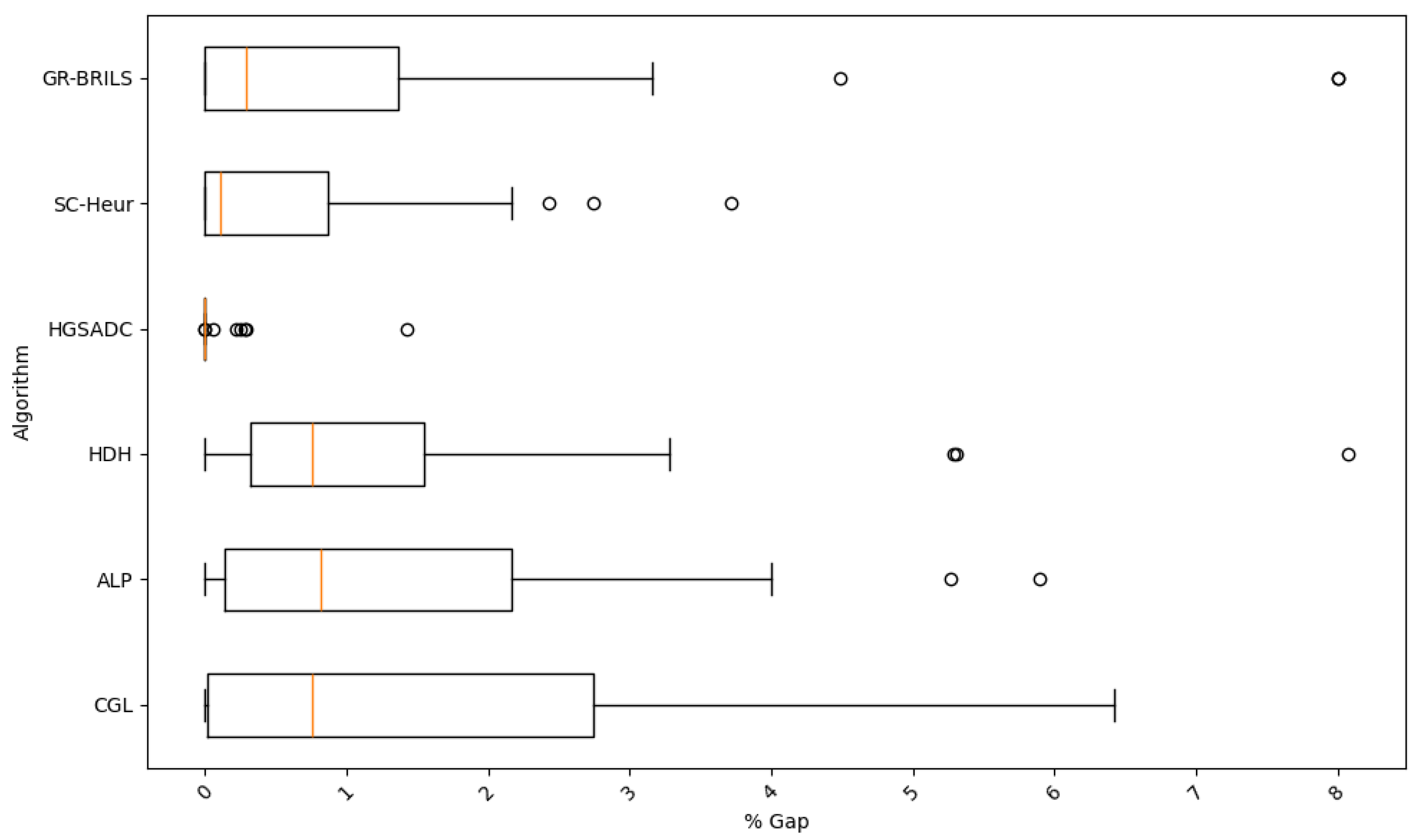
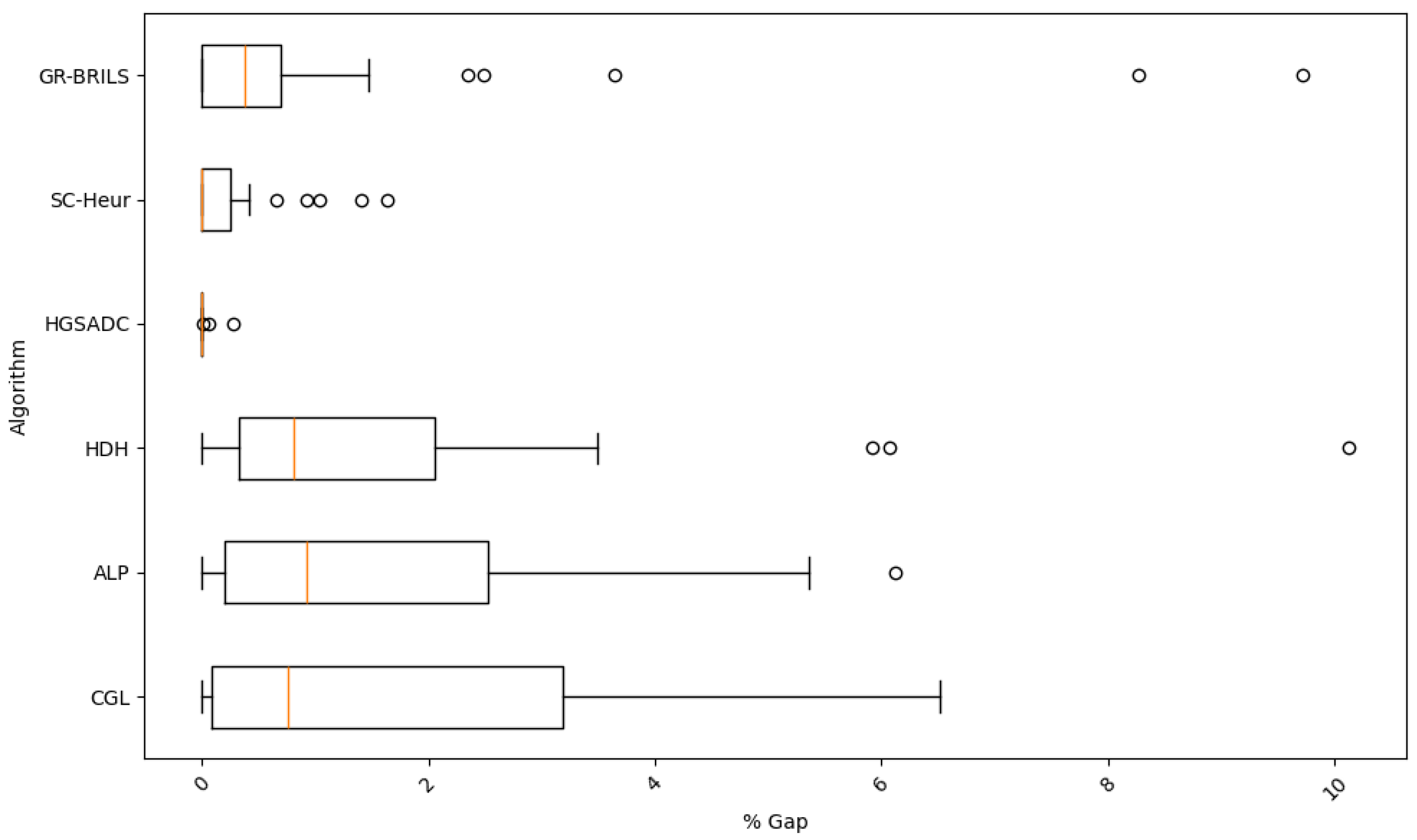
Across the full benchmark set, the proposed GR-BRILS reaches an average deviation of $1.18\%$ from the best value obtained in each case. This places it comfortably ahead of the constructive heuristics CGL ($1.56\%$), ALP ($1.33\%$) and HDH ($1.36\%$). Compared with the two competing metaheuristics, GR-BRILS remains competitively close; it is only $0.64$ percentage points behind SC-Heur ($0.54\%$) and $1.04$ points behind HGADC ($0.14\%$), a gap that is operationally modest given the scale of the problem. A closer inspection of the instance groups reveals that the three metaheuristics behave virtually identically on the small and medium cases (p01 to p26), all staying below the one-percent line. The decisive evidence in favor of GR-BRILS emerges in the largest and most demanding subset (p27 to p32). In that group, it registers an average gap of just $0.15\%$, almost identical to HGADC ($0.13\%$) and clearly better than SC-Heur ($0.27\%$). In addition, GR-BRILS achieves the best objective value in two of the largest and most challenging instances, namely p30 and p32, demonstrating its competitiveness in particularly demanding scenarios. Overall, the results confirm that GR-BRILS is a highly effective method for solving the PVRP, particularly for larger-scale problems where its improvements are most evident. The algorithm therefore offers a compelling combination of scalability, consistency, and solution quality that makes it a strong candidate for large-scale periodic vehicle routing applications.

On the other hand, we also analyze the best values obtained in Table 3. The results show a similar performance ranking, once again highlighting the proposed GR-BRILS algorithm on large-scale instances, with a 0.33% gap relative to the BKS, largely contributed by HGADC, with an average gap of 0.01% for this indicator. However, in this case, there is a larger difference with the SC-Heur algorithm.

To study the results visually, Figure 5 and Figure 6 present box-plots that provide a comprehensive view of the outcomes. It can be observed that the proposed algorithm achieves the third-best performance in both indicators, although it exhibits very pronounced outliers. These outliers appear in instances with very tight capacity constraints (p11 to p13), where the map generation process struggles to find feasible solutions.

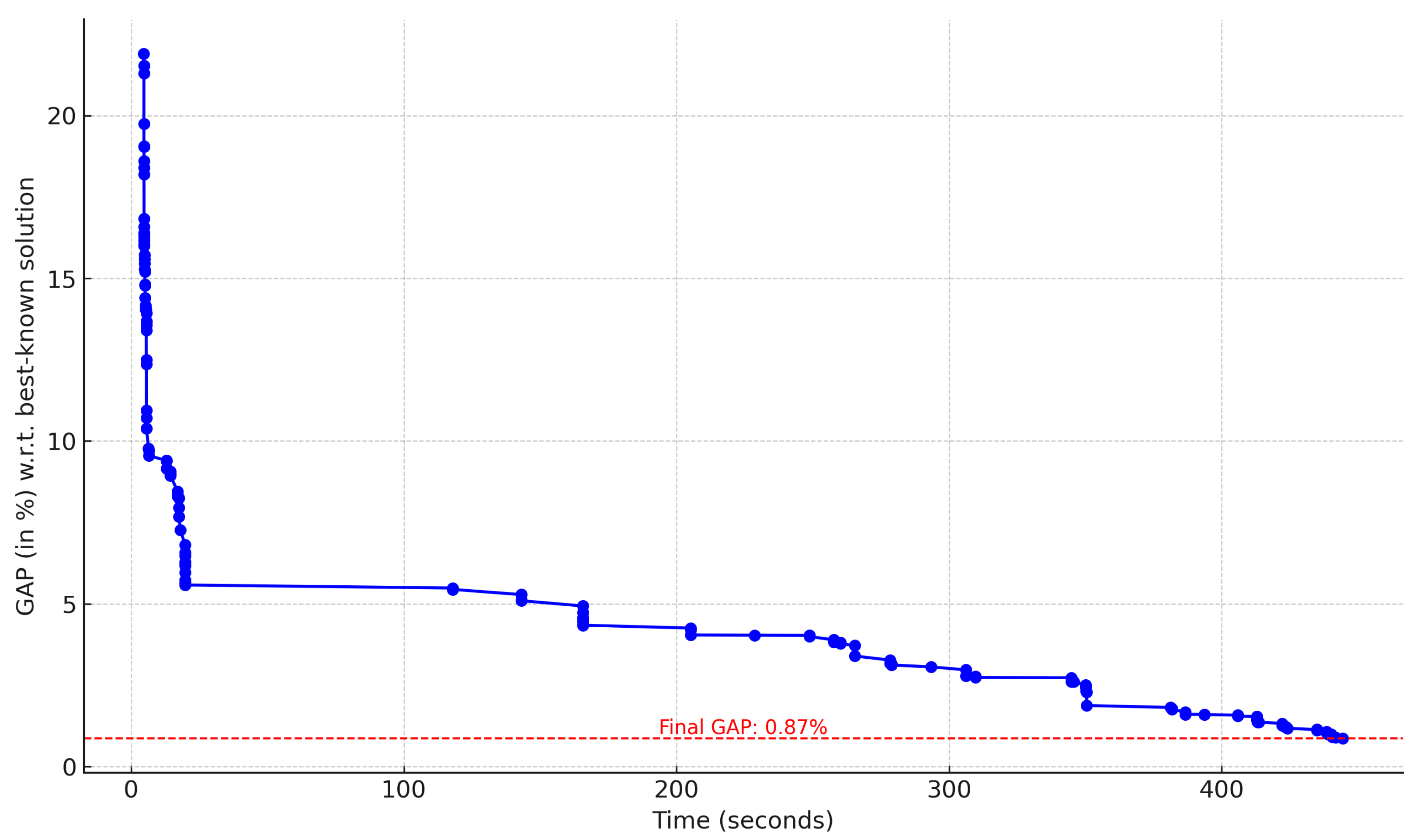
To examine the search dynamics in more detail, we carried out an example run on instances p01 and p27. As shown in the following figures, each loop begins with a biased–randomized round-robin constructor that generates a feasible solution in approximately two seconds, followed by the described iterated local search procedure.

We observed particularly fast convergence on the smaller instances. Instance p01 (Figure 7) reached a gap of 0.00% with respect to the best known solution in approximately 50 and 2 s, respectively. This illustrates the efficiency of the algorithm in rapidly identifying high-quality solutions. For larger instances such as p27 (Figure 8), the algorithm showed a more continuous improvement over time. The algorithm reached a gap of 0.87% percent after 7 min. These examples illustrate how once the round-robin mechanism produces an initial feasible solution, the algorithm continues to improve it, progressively, through the ILS phase. This efficient construction phase demonstrates the effectiveness of the biased–randomized strategy in providing a strong starting point for the optimization process.

Statistical Significance of the Results

To obtain an initial global view of the results, we performed a one-way analysis of variance (ANOVA) on the minimum gaps reported in Table 3. The test yielded $F(5,186)=6.08$ with $p=3.1\times {10}^{-5}$, so the null hypothesis of equal mean gaps is clearly rejected, and at least one algorithm performs differently from the rest. Guided by this result, we next examine which specific pairs drive the observed differences.

To explore these differences in more detail, Tukey’s honestly significant difference (HSD) test at $\alpha =0.05$ was applied to identify which algorithm pairs contribute to the overall effect.

Table 4. Tukey’s HSD on minimum relative gaps (%).

Pair	$\mathit{\Delta }\overline{\mathit{g}}$	95% CI	${\mathit{p}}_{\mathbf{adj}}$	Decision
ALP–HGADC	$-1.60$	$(-2.87,-0.33)$	0.005	different
ALP–SC-Heur	$-1.29$	$(-2.56,-0.02)$	0.045	different
CGL–HGADC	$-1.84$	$(-3.10,-0.57)$	0.001	different
CGL–SC-Heur	$-1.53$	$(-2.79,-0.27)$	0.008	different
HDH–HGADC	$-1.64$	$(-2.90,-0.38)$	0.003	different
HDH–SC-Heur	$-1.33$	$(-2.59,-0.07)$	0.032	different
ALP–CGL	$0.24$	$(-1.03,1.51)$	0.994	equal
ALP–GR-BRILS	$-0.42$	$(-1.69,0.85)$	0.931	equal
ALP–HDH	$0.04$	$(-1.23,1.31)$	1.000	equal
CGL–GR-BRILS	$-0.66$	$(-1.92,0.60)$	0.659	equal
CGL–HDH	$-0.20$	$(-1.46,1.07)$	0.998	equal
GR-BRILS–HDH	$0.47$	$(-0.80,1.73)$	0.895	equal
GR-BRILS–HGADC	$-1.17$	$(-2.44,0.09)$	0.083	equal
GR-BRILS–SC-Heur	$-0.87$	$(-2.13,0.40)$	0.359	equal
HGADC–SC-Heur	$0.31$	$(-0.95,1.57)$	0.981	equal

presents the adjusted p-values ($p_{\mathrm{adj}}$). Six contrasts are statistically significant, and in each case, either HGADC or SC-Heur achieves superior performance over ALP, CGL, or HDH. No comparison that involves GR-BRILS is significant, implying that the proposed method is statistically equivalent to the two best state-of-the-art heuristics while being considerably simpler to implement. These statistical findings confirm that GR-BRILS achieves the same level of solution quality as the best available heuristics, despite relying on a much simpler search scheme.

7. Conclusions and Future Work

This paper introduced a novel two-phase approach for addressing a rich variant of the periodic vehicle routing problem. The first phase builds a feasible day–vehicle assignment in seconds through a round-robin construction that enforces customer frequencies. The second phase refines those assignments with local search restricted to single-day routes, combined with cross-day perturbations accepted under a simulated annealing rule. The interaction of these phases gives the method the ability to scale to instances with many thousands of nodes while keeping computational times practical.

A key strength of our methodology lies in its simplicity and scalability. By prioritizing feasibility and coverage in the early stage, the algorithm constructs an initial solution efficiently even for very large instances. The subsequent improvement phase iterates between short, focused local search steps and inter-day perturbations, producing a balanced equilibrium between intensification and diversification. While performance on small and medium problems is on par with leading methods, the gap in both solution quality and the overall computational effort increases significantly in our favor on the largest benchmark cases, underscoring the approach’s particular suitability for large-scale routing applications. In comparison to the HGADC algorithm, which achieves state-of-the-art results, the algorithm proposed in this work has a simple implementation process and offers greater explainability, as it is a constructive algorithm with very clear criteria. Moreover, it provides feasible solutions in very short times from the very first biased–randomized round-robin phase, unlike a genetic algorithm, which carries a higher risk in that regard.

Future work will focus on several enhancements that aim to expand both the practical and theoretical reach of our approach. First, we plan to incorporate additional real-world constraints such as time windows, driver consistency, and dynamic travel times, which were not tested in this study and therefore represent natural extensions to better reflect day-to-day operational realities. Second, we will explore an adaptive search framework, where parameters and neighborhood operators adjust in real time based on the solution’s progress. Finally, we intend to integrate simheuristics that account for uncertainty—for example, in travel times or demands—so that solutions become more robust to disruptions or unexpected changes.