Existence Results for Nabla Fractional Problems with Anti-Periodic Boundary Conditions

Abstract

The aim of this work is to study a class of nabla fractional difference equations with anti-periodic conditions. First, we construct the related Green’s function. After deducing some of its useful properties, we obtain an upper bound for its sum. Then, using this bound, we are able to obtain three existence results based on the Banach contraction principle, Brouwer’s fixed point theorem, and Leray–Schauder’s nonlinear alternative, respectively. Then, we show some non-existence results for the studied problem, and existence results are also provided for a system of two equations of the considered type. Finally, we outline some particular examples in order to demonstrate the theoretical findings.

1. Introduction

Since the models described with fractional orders proved out to be much more accurate in comparison to those with integer orders, this concept has become fundamental in many areas of mathematics in the recent few decades. Consequently, the interest in discrete fractional problems has recently surged. They are applicable in numerous branches of engineering and science, including signal processing, control theory, and mathematical modeling of phenomena in economics, biology, and physics, where discrete events or data points are predominant. We refer to the reader [1,2,3,4] and the references therein for an introduction to the fundamentals of this subject.

Usually, nabla fractional models better describe some long-term memory effects [5,6,7], which make them highly suitable for modeling non-local processes in time or space. As a result, a lot of recent papers focused on nabla problems with different boundary conditions, like Dirichlet [8,9,10,11,12], periodic [13], mixed [14,15,16], summation [17] and separated boundary conditions [18,19] or systems [10,20,21,22].

For example, in [18], the authors studied the following nabla fractional problem with separated boundary conditions:

$$\begin{array}{c}-\left({\nabla }_a^{\upsilon -1}\left(\nabla u\right)\right)\left(\xi \right)+g\left(\xi \right)u\left(\left(\xi \right)\right)=f\left(\xi ,u\left(\xi \right)\right),\xi \in {\mathbb{N}}_{a+2}^b,\\ \alpha u\left(a+1\right)-\beta \left(\nabla u\right)\left(a+1\right)=0,\gamma u\left(b\right)+\delta \left(\nabla u\right)\left(b\right)=0,\end{array}$$

where $a,b\in \mathbb{R}$, $1<\upsilon <2$, $g:{\mathbb{N}}_{a+2}^b\to \mathbb{R}$, $f:{\mathbb{N}}_{a+2}^b\times \mathbb{R}\to \mathbb{R}$, and ${\nabla }_a^{\upsilon -1}$ denotes the $\upsilon -1$-th-order Riemann–Liouville nabla difference operator, $\alpha ,\beta ,\gamma ,\delta \in R$ with ${\alpha }^2+{\beta }^2>0$ and ${\gamma }^2+{\delta }^2>0$. The associated Green’s function is constructed as a series of functions with the help of spectral theory, and some of its properties are obtained. Under suitable conditions on the nonlinear part of the problem, the authors managed to deduce two existence results by means of fixed-point theory.

Later, in [17], the authors studied the nabla fractional problem coupled with summation conditions:

$$\begin{array}{c}-\left({\nabla }_{\rho \left(a\right)}^{\upsilon }u\right)\left(\xi \right)=f\left(\xi ,u\left(\xi \right)\right),\xi \in {\mathbb{N}}_{a+2}^b,\\ u\left(a\right)=A,u\left(b\right)+\mu \sum _{s=a+1}^{b-1}u\left(s\right)=B,\end{array}$$

where $a,b,A,B\in \mathbb{R}$, $\mu >0$, $u:{\mathbb{N}}_{a+2}^b\to \mathbb{R}$, $f:{\mathbb{N}}_{a+2}^b\times \mathbb{R}\to \mathbb{R}$, is continuous with respect to the second argument; $1<\upsilon <2$ and ${\nabla }_{\rho \left(a\right)}^{\upsilon }u$ denotes the ${\upsilon }^{\mathrm{th}}$-order Riemann–Liouville nabla fractional difference. Under some sufficient conditions, the authors ensured existence and uniqueness results. Moreover, the obtained solution is generalized Ulam–Hyers–Rassias-stable.

Recently, in [16] the authors studied the nabla fractional problem

$$\begin{array}{c}-\left({\nabla }_{\rho \left(a\right)}^{\upsilon }u\right)\left(\xi \right)=\lambda f\left(\xi \right)g\left(u\left(\xi \right)\right),\xi \in {\mathbb{N}}_{a+2}^b,\\ u\left(a\right)=\left({\nabla }_{\rho \left(b\right)}^{\mu }u\right)\left(b\right)=0,\end{array}$$

where $f:{\mathbb{N}}_{a+2}^b\to \left(0,\infty \right)$ and $g:\left[0,\infty \right)\to g:\left[0,\infty \right)$ are continuous functions, while $0\le \mu \le 1<\upsilon <2$, ${\nabla }_{\rho \left(a\right)}^{\upsilon }$ and ${\nabla }_{\rho \left(b\right)}^{\mu }$ are $\upsilon$th- and $\mu$th-order nabla difference operators of the Riemann–Liouville type, respectively. Depending on the values of the orders of the operators, the authors split their research into two main cases, and for each one of them, they managed to prove that the considered problem possesses a positive solution.

In [10], the author obtained the unique existing solution of the systems

$$\begin{array}{c}-\left({\nabla }_0^{{\alpha }_1-1}\left(\nabla u_1\right)\right)\left(t\right)+f_1\left(t,u_1\left(t\right),u_2\left(t\right)\right)=0,t\in {\mathbb{N}}_2^T,\\ -\left({\nabla }_0^{{\alpha }_2-1}\left(\nabla u_1\right)\right)\left(t\right)+f_2\left(t,u_1\left(t\right),u_2\left(t\right)\right)=0,t\in {\mathbb{N}}_2^T,\\ u_1\left(0\right)+u_1\left(T\right)=\left(\nabla u_1\right)\left(1\right)+\left(\nabla u_1\right)\left(T\right)=0,\\ u_2\left(0\right)+u_2\left(T\right)=\left(\nabla u_2\right)\left(1\right)+\left(\nabla u_2\right)\left(T\right)=0,\end{array}$$

where $T\in {\mathbb{N}}_2$, ${\alpha }_1,{\alpha }_2\in \left(1,2\right)$ and $f_1,f_2:{\mathbb{N}}_0^T\times {\mathbb{R}}^2\to \mathbb{R}$ are continuous, and deemed that it is Ulam–Hyers-stable.

Inspired by the aforementioned works, this study considered the nabla fractional problem with a Riemann–Liouville operator and anti-periodic conditions:

$$\begin{array}{c}-\left({\nabla }_{\rho \left(m\right)}^{\nu }u\right)\left(\xi \right)=\mathfrak{f}(\xi ,u\left(\xi \right)),\xi \in {\mathbb{N}}_{m+2}^n\equiv I,\end{array}$$

(1)

$$\begin{array}{c}u\left(m\right)+u\left(n\right)=0,\left(\nabla u\right)(m+1)+\left(\nabla u\right)\left(n\right)=0,\end{array}$$

(2)

where $1<\nu \le 2$, $n,m\in \mathbb{N}$ with $m+2<n$, ${\nabla }_{\rho \left(m\right)}^{\nu }u$ denotes the ${\nu }^{\mathrm{th}}$-order Riemann–Liouville nabla fractional difference of u in $\rho \left(m\right)=m-1$ and $\mathfrak{f}:I\times \mathbb{R}\to \mathbb{R}$ is continuous.

We point out that these conditions have a clear physical representation, as they imply that total “displacement” across the domain is balanced, with the gradient (velocity, flux, and related physical quantities) entering at the point $m+1$ and exiting at the point n also being balanced. Such conditions arise in real-life problems, where discrete fractional oscillators or some models in biology with memory effects are studied. Moreover, discrete fractional boundary value problems involve finding solutions to fractional difference equations that satisfy prescribed conditions at more than one point, typically at the endpoints of a discrete interval. Among the various types of boundary conditions, antiperiodic boundary conditions are of particular interest because of their broad applicability. Antiperiodic boundary value problems model phenomena in which the system returns to a state, i.e., the negative of its initial condition after a fixed period are useful in describing alternating current systems and certain waveforms. Establishing existence and uniqueness results for such boundary value problems is not only of theoretical interest but is also crucial for practical implementation. These results provide the foundational assurance that the mathematical models used to represent real-world phenomena are both well-posed and solvable. They also pave the way for the development of efficient numerical methods and simulations. In this context, the present study contributes to the theoretical framework of discrete fractional calculus and improves its applicability in modeling complex discrete dynamic systems.

We also refer to the reader to [23,24], where some singular stochastic problems are considered, along with some numerical methods for heat model arising in viscoelasticity.

Also note that the arguments in our manuscript are different from those given in [10]. Although the boundary conditions considered in both problems are the same, there is a clear distinction between the fractional difference equations considered in both works since both operators do not coincide. That is,

$$\left({\nabla }_m^{\nu -1}\left(\nabla u\right)\right)\left(\xi \right)\ne \left({\nabla }_{m-1}^{\nu }u\right)\left(\xi \right).$$

These operators coincide if $u\left(m\right)=0$. In such a case, both boundary value problems are ill-posed. Moreover, in this manuscript, we study an anti-periodic problem with a different fractional difference equation in contrast to the fractional difference equations considered in [10]. So, we need to define a different operator and a cone, where our aim is to deduce the existence of a fixed point. Consequently, the results obtained in our manuscript are completely different from those obtained in [10]. Furthermore, since the boundary value problems considered in both works are completely different, this manuscript presents novel results.

We point out that the only limitation of this work is the fact that only a sign-changing solution could be obtained, based on the non-constant sign of Green’s function, which is typical for problems coupled with anti-periodic conditions, such as (2), and this limitation could not be resolved.

As novel contributions to the work, we can highlight the following:

• The boundary value problem (1)–(2) considered in this work is completely different from the one given in [10].
• We deduced the exact expression of Green’s function associated with (1)–(2) and obtained the upper bound for its sum.
• We established existence and non-existence results for (1)–(2) under some sufficient conditions.
• We established some existence results for a system of two equations corresponding to (1)–(2).
• We provided some examples to illustrate the main results for this new problem for the literature.

This manuscript is structured as follows: Section 2 recalls the preliminaries required for the article. Section 3 deduces the exact expression of Green’s function that is associated with (1)–(2), and the upper bound of its sum is obtained. After that, in Section 4, under certain sufficient conditions, two existence results are established for problem (1)–(2) using the Banach contraction principle, Brouwer theorem and Leray–Schauder’s nonlinear alternative, respectively. In Section 5, non-existence results are demonstrated, and in Section 6, existence results are provided for a system of two equations. Finally, the theoretical results are illustrated in Section 7, as some examples are shown there to highlight their practical value. In the Conclusions Section, we finish with a brief summary of our obtained results and some possible future directions for extending this research.

2. Preliminaries

To the end of this work, we shall use the following fundamentals of discrete fractional calculus [4], which are represented as ${\mathbb{N}}_{\kappa }=\{\kappa ,\kappa +1,\kappa +2,\dots \}$, ${\mathbb{N}}_{\kappa }^{\varkappa }=\{\kappa ,\kappa +1,\kappa +2,\dots ,\varkappa \}$. Here, $\kappa$, $\varkappa \in \mathbb{R}$ with $\varkappa -\kappa \in {\mathbb{N}}_1$.

Definition 1

([4]). For any α, $\beta \in \mathbb{R}$, the generalized rising function is

$${\alpha }^{\overline{\beta }}={\displaystyle \frac{\Gamma (\alpha +\beta )}{\Gamma \left(\alpha \right)}},$$

provided the quotient is well-defined, with $\Gamma \left(z\right)={\int }_0^{\infty }{t}^{z-1}{e}^{-t}dt$ being the Euler gamma function for those complex numbers z for which the real part of z is positive.

Definition 2

([4]). Let $\gamma \in \mathbb{R}\setminus \{\dots ,-2,-1\}$. The ${\gamma }^{th}$-order nabla fractional Taylor monomial is

$${\mathfrak{h}}_{\gamma }(\zeta ,k)={\displaystyle \frac{{(\zeta -k)}^{\overline{\gamma }}}{\Gamma (\gamma +1)}},$$

provided the right-hand side is well-defined.

Lemma 1

([4]). Take $s\in {\mathbb{N}}_k$ and $\gamma >-1$.

(i) 

${\mathfrak{h}}_{\gamma }(\zeta ,s-1)\ge 0$ for $\zeta \in {\mathbb{N}}_{s-1}$ and ${\mathfrak{h}}_{\gamma }(\zeta ,s-1)>0$ for $\zeta \in {\mathbb{N}}_s$;

(ii) 

${\mathfrak{h}}_{\gamma }(\zeta ,s-1)$ decreases with respect to s for any $\zeta \in {\mathbb{N}}_{s-1}$ and $\gamma >0$. Moreover, it decreases with respect to ζ for any $\zeta \in {\mathbb{N}}_s$ and $\gamma >0$.

Definition 3

([4]). Let $w:{\mathbb{N}}_{k+1}\to \mathbb{R}$. The ${\eta }^{\mathit{th}}$, $\eta >0$, fractional difference of w in the nabla sense is

$$\left({\nabla }_k^{\eta }w\right)\left(\zeta \right)=\left({\nabla }^N\left({\nabla }_k^{-(N-\eta )}w\right)\right)\left(\zeta \right),N\in {\mathbb{N}}_1,N-1<\eta \le N,\zeta \in {\mathbb{N}}_{k+N}.$$

We will mainly use the following well-known classical results in this work, the Banach contraction principle, Brouwer theorem, and Leray–Schauder’s nonlinear alternative, respectively, which can be found in [25].

Theorem 1.

A contraction mapping on a complete metric space has exactly one fixed point.

Theorem 2.

Let X be a nonempty, bounded, closed and convex set. Moreover, if $F:X\to X$ is a continuous mapping, then F has a fixed point.

Theorem 3.

Let $\mathcal{B}=\left(\mathcal{B},\parallel ·\parallel \right)$ be a Banach space, C a closed, convex subset of $\mathcal{B}$, U an open subset of C, and $0\in U$. Suppose that $T:\overline{U}\to C$ is a completely continuous map. Then, either of the two is possible:

1. 

T has a fixed point in $\overline{U}$;

2. 

There exist $y\in \partial U$ and $\lambda \in (0,1)$ such that $y=\lambda Ty$.

3. Construction and Properties of Green’s Function

The following section presents the construction of Green’s function for the linear problem and deduces some of its useful properties, which we will need at the end of this work.

$$-\left({\nabla }_{\rho \left(m\right)}^{\nu }u\right)\left(\xi \right)=\mathfrak{g}\left(\xi \right),\xi \in I,$$

(3)

coupled with boundary conditions (2). Here, $\mathfrak{g}:I\to \mathbb{R}$. For this purpose, we introduce the following notation:

$$\begin{array}{ccc}\hfill \Lambda & =& {\mathfrak{h}}_{\nu -3}(n,\rho \left(m\right))+\nu {\mathfrak{h}}_{\nu -1}(n,m)+{\displaystyle \frac{(n-m){\mathfrak{h}}_{\nu -2}(n,\rho \left(m\right)){\mathfrak{h}}_{\nu -3}(n,\rho \left(m\right))}{(\nu -1)(2-\nu )}}\hfill \\ & & -2{\mathfrak{h}}_{\nu -1}(n,\rho \left(m\right))-1,\hfill \\ \hfill \varphi \left(s\right)& =& -{\mathfrak{h}}_{\nu -2}(n,\rho \left(s\right))+{\displaystyle \frac{\left[n-m(\nu -1)-s(2-\nu )\right]{\mathfrak{h}}_{\nu -2}(n,\rho \left(s\right)){\mathfrak{h}}_{\nu -3}(n,\rho \left(m\right))}{(\nu -1)(2-\nu )}}\hfill \\ & & -(2-\nu ){\mathfrak{h}}_{\nu -1}(n,\rho \left(s\right)),\hfill \\ \hfill \psi \left(s\right)& =& {\mathfrak{h}}_{\nu -2}(n,\rho \left(s\right))+{\displaystyle \frac{(s-m){\mathfrak{h}}_{\nu -2}(n,\rho \left(m\right)){\mathfrak{h}}_{\nu -2}(n,\rho \left(s\right))}{(\nu -1)}}-(\nu -1){\mathfrak{h}}_{\nu -1}(n,\rho \left(s\right)).\hfill \end{array}$$

Theorem 4.

Assume $\Lambda \ne 0$. There exists a unique solution of (3)–(2) in the form

$$u\left(\xi \right)=\sum _{s\in I}\mathcal{G}(\xi ,s)\mathfrak{g}\left(s\right),\xi \in {\mathbb{N}}_m^n,$$

(4)

where

$$\mathcal{G}(\xi ,s)=\left\{\begin{array}{c}{\mathcal{G}}_1(\xi ,s),\xi \in {\mathbb{N}}_m^{\rho \left(s\right)},\hfill \\ {\mathcal{G}}_2(\xi ,s),\xi \in {\mathbb{N}}_s^n,\hfill \end{array}\right.$$

(5)

with

$${\mathcal{G}}_1(\xi ,s)={\displaystyle \frac{\varphi \left(s\right){\mathfrak{h}}_{\nu -1}(\xi ,\rho \left(m\right))+\psi \left(s\right){\mathfrak{h}}_{\nu -2}(\xi ,\rho \left(m\right))}{\Lambda }},$$

and

$${\mathcal{G}}_2(\xi ,s)={\mathcal{G}}_1(\xi ,s)-{\mathfrak{h}}_{\nu -1}(\xi ,\rho \left(s\right)).$$

Proof. 

It is well-known [4] that the general solution of (3) can be expressed as

$$u\left(\xi \right)=D_1{\mathfrak{h}}_{\nu -1}(\xi ,\rho \left(m\right))+D_2{\mathfrak{h}}_{\nu -2}(\xi ,\rho \left(m\right))-\left({\nabla }_{m+1}^{-\nu }\mathfrak{g}\right)\left(\xi \right),\xi \in {\mathbb{N}}_m^n,$$

(6)

with $D_1$ and $D_2$ being arbitrary constants. By applying ∇ on the above equation, we obtain

$$\left(\nabla u\right)\left(\xi \right)=D_1{\mathfrak{h}}_{\nu -2}(\xi ,\rho \left(m\right))+D_2{\mathfrak{h}}_{\nu -3}(\xi ,\rho \left(m\right))-\left({\nabla }_{m+1}^{1-\nu }\mathfrak{g}\right)\left(\xi \right),\xi \in {\mathbb{N}}_{m+1}^n.$$

Using $u\left(m\right)+u\left(n\right)=0$, we get

$$\left[1+{\mathfrak{h}}_{\nu -1}(n,\rho \left(m\right))\right]D_1+\left[1+{\mathfrak{h}}_{\nu -2}(n,\rho \left(m\right))\right]D_2=\sum _{s\in I}{\mathfrak{h}}_{\nu -1}(n,\rho \left(s\right))\mathfrak{g}\left(s\right).$$

(7)

Similarly, by $\left(\nabla u\right)(m+1)+\left(\nabla u\right)\left(n\right)=0$, we obtain

$$\left[\nu -1+{\mathfrak{h}}_{\nu -2}(n,\rho \left(m\right))\right]D_1+\left[\nu -2+{\mathfrak{h}}_{\nu -3}(n,\rho \left(m\right))\right]D_2=\sum _{s\in I}{\mathfrak{h}}_{\nu -2}(n,\rho \left(s\right))\mathfrak{g}\left(s\right).$$

(8)

From (7) and (8), we have

$$D_1={\displaystyle \frac{1}{\Lambda }}\sum _{s\in I}\varphi \left(s\right)\mathfrak{g}\left(s\right),$$

(9)

and

$$D_2={\displaystyle \frac{1}{\Lambda }}\sum _{s\in I}\psi \left(s\right)\mathfrak{g}\left(s\right).$$

(10)

By substituting (9) and (10) in (6), we obtain (4). □

Now, set

$$\begin{array}{ccc}\hfill L\left(\xi \right)& =& {\displaystyle \frac{{\mathfrak{h}}_{\nu -1}(\xi ,\rho \left(m\right)){\mathfrak{h}}_{\nu -2}(n,m+1)}{\left|\Lambda \right|}}\left(1+{\displaystyle \frac{\left(n-m\right){\mathfrak{h}}_{\nu -3}(n,m-1)}{2-\nu }}\right)\hfill \\ & & +{\displaystyle \frac{(2-\nu ){\mathfrak{h}}_{\nu -1}(n,m+1)}{\left|\Lambda \right|}}\hfill \\ & & +{\displaystyle \frac{{\mathfrak{h}}_{\nu -2}(\xi ,\rho \left(m\right)){\mathfrak{h}}_{\nu -2}(n,m+1)}{\left|\Lambda \right|}}\left(1+{\displaystyle \frac{(n-m){\mathfrak{h}}_{\nu -2}(n,m-1)}{\nu -1}}\right)\hfill \\ & & +{\displaystyle \frac{(\nu -1){\mathfrak{h}}_{\nu -1}(n,m+1)}{\left|\Lambda \right|}}+{\mathfrak{h}}_{\nu -1}(n,m+1),\xi \in {\mathbb{N}}_m^n\hfill \end{array}$$

and

$$L=\underset{\xi \in {\mathbb{N}}_m^n}{max}L\left(\xi \right).$$

Lemma 2.

For $\mathcal{G}\left(\xi ,s\right)$ given in (5), we have the upper bound

$$\sum _{s\in I}\left|\mathcal{G}\left(\xi ,s\right)\right|\le L.$$

Proof. 

Using

$$\sum _{s=m+2}^p{\mathfrak{h}}_{\nu -1}(p,s-1)={\mathfrak{h}}_{\nu -1}(p,m+1),$$

we have that

$$\begin{array}{ccc}\hfill \sum _{s\in I}\left|\mathcal{G}\left(\xi ,s\right)\right|& =& \sum _{s=m+2}^{\xi }\left|{\mathcal{G}}_1\left(\xi ,s\right)-{\mathfrak{h}}_{\nu -1}(\xi ,s-1)\right|+\sum _{s=\xi +1}^n\left|{\mathcal{G}}_1\left(\xi ,s\right)\right|\hfill \\ & \le & \sum _{s\in I}\left|{\mathcal{G}}_1\left(\xi ,s\right)\right|+\sum _{s=m+2}^{\xi }{\mathfrak{h}}_{\nu -1}(\xi ,s-1)\hfill \\ & \le & {\displaystyle \frac{{\mathfrak{h}}_{\nu -1}(\xi ,\rho \left(m\right))}{\left|\Lambda \right|}}\sum _{s\in I}\left|\varphi \left(s\right)\right|+{\displaystyle \frac{{\mathfrak{h}}_{\nu -2}(\xi ,\rho \left(m\right))}{\left|\Lambda \right|}}\sum _{s\in I}\left|\psi \left(s\right)\right|+{\mathfrak{h}}_{\nu -1}(\xi ,m+1).\hfill \end{array}$$

Note that $n-m(\nu -1)-s(2-\nu )\le \left(n-m\right)(\nu -1)$ since the left-hand side is positive and decreasing for $s\in I$. Thus,

$$\begin{array}{ccc}\hfill \sum _{s\in I}\left|\varphi \left(s\right)\right|& \le & \sum _{s\in I}{\mathfrak{h}}_{\nu -2}(n,s-1)+(2-\nu )\sum _{s\in I}{\mathfrak{h}}_{\nu -1}(n,s-1){\mathfrak{H}}_{\nu -2}(n,s-1)\hfill \\ & & +{\displaystyle \frac{{\mathfrak{h}}_{\nu -3}(n,m-1)}{(\nu -1)(2-\nu )}}\sum _{s\in I}\left[n-m(\nu -1)-s(2-\nu )\right]\hfill \\ & =& {\mathfrak{h}}_{\nu -2}(n,m+1)\left(1+{\displaystyle \frac{\left(n-m\right){\mathfrak{h}}_{\nu -3}(n,m-1)}{2-\nu }}\right)+(2-\nu ){\mathfrak{h}}_{\nu -1}(n,m+1).\hfill \end{array}$$

Similarly, since $s\le n$,

$$\begin{array}{ccc}\hfill \sum _{s\in I}\left|\psi \left(s\right)\right|& \le & \sum _{s\in I}{\mathfrak{h}}_{\nu -2}(n,s-1)+{\displaystyle \frac{(n-m){\mathfrak{h}}_{\nu -2}(n,m-1)}{\nu -1}}\sum _{s\in I}{\mathfrak{h}}_{\nu -2}(n,s-1)\hfill \\ & & +(\nu -1)\sum _{s\in I}{\mathfrak{h}}_{\nu -1}(n,s-1)\hfill \\ & =& {\mathfrak{h}}_{\nu -2}(n,m+1)\left(1+{\displaystyle \frac{(n-m){\mathfrak{h}}_{\nu -2}(n,m-1)}{\nu -1}}\right)+(\nu -1){\mathfrak{h}}_{\nu -1}(n,m+1).\hfill \end{array}$$

Finally, using ${\mathfrak{h}}_{\nu -1}(\xi ,m+1)\le {\mathfrak{h}}_{\nu -1}(n,m+1)$, we deduce

$$\begin{array}{ccc}\hfill \sum _{s\in I}\left|\mathcal{G}\left(\xi ,s\right)\right|& \le & {\displaystyle \frac{{\mathfrak{h}}_{\nu -1}(\xi ,\rho \left(m\right)){\mathfrak{h}}_{\nu -2}(n,m+1)}{\left|\Lambda \right|}}\left(1+{\displaystyle \frac{\left(n-m\right){\mathfrak{h}}_{\nu -3}(n,m-1)}{2-\nu }}\right)\hfill \\ & & +{\displaystyle \frac{(2-\nu ){\mathfrak{h}}_{\nu -1}(n,m+1)}{\left|\Lambda \right|}}\hfill \\ & & +{\displaystyle \frac{{\mathfrak{h}}_{\nu -2}(\xi ,\rho \left(m\right)){\mathfrak{h}}_{\nu -2}(n,m+1)}{\left|\Lambda \right|}}\left(1+{\displaystyle \frac{(n-m){\mathfrak{h}}_{\nu -2}(n,m-1)}{\nu -1}}\right)\hfill \\ & & +{\displaystyle \frac{(\nu -1){\mathfrak{h}}_{\nu -1}(n,m+1)}{\left|\Lambda \right|}}+{\mathfrak{h}}_{\nu -1}(n,m+1),\hfill \end{array}$$

which proves our claim. □

4. Existence Results

Let $\mathfrak{B}$ be the Banach space of all continuous functions $\left\{u:I\to \mathbb{R}\right\}$ with the standard maximum norm

$$∥u∥=\underset{\xi \in I}{max}\left|u\left(\xi \right)\right|.$$

For each $\xi \in I$, define the operator $\mathfrak{T}:\mathfrak{B}\to \mathfrak{B}$ by

$$\left(\mathfrak{T}u\right)\left(\xi \right)=\sum _{s\in I}\mathcal{G}\left(\xi ,s\right)\mathfrak{f}\left(s,u\left(s\right)\right).$$

The first key results of our work are as follows:

Theorem 5.

If there exists $L_1\in \left(0,{\displaystyle \frac{1}{L}}\right)$ such that

$$\left|\mathfrak{f}\left(\xi ,v\right)-\mathfrak{f}\left(\xi ,w\right)\right|\le L_1\left|v-w\right|,$$

for each $\xi \in I$ and all $v,w\in \mathfrak{B}$, then (1)–(2) has a unique solution in $\mathfrak{B}$.

Proof. 

Let $v,w\in \mathfrak{B}$. Then, for each $\xi \in I$, one can deduce that

$$\begin{array}{ccc}\hfill \left|\mathfrak{T}v\left(\xi \right)-\mathfrak{T}w\left(\xi \right)\right|& =& \left|\sum _{s\in I}\mathcal{G}\left(\xi ,s\right)\mathfrak{f}\left(s,v\left(s\right)\right)-\sum _{s\in I}\mathcal{G}\left(\xi ,s\right)\mathfrak{f}\left(s,w\left(s\right)\right)\right|\hfill \\ & \le & \sum _{s\in I}\left|\mathcal{G}\left(\xi ,s\right)\right|\left|\mathfrak{f}\left(s,v\left(s\right)\right)-\mathfrak{f}\left(s,w\left(s\right)\right)\right|\hfill \\ & \le & L{L}_1∥v-w∥\hfill \\ & <& ∥v-w∥.\hfill \end{array}$$

Hence, $∥\mathfrak{T}v-\mathfrak{T}w∥<∥v-w∥$, which gives us that the operator is a contraction; therefore, by Theorem 1, its unique fixed point is the unique solution of the considered problem (1)–(2). □

Theorem 6.

Suppose that there exists a bounded function $\mathfrak{F}:I\to \mathbb{R}$ such that

$$\underset{\xi \in I}{max}\mathfrak{F}\left(\xi \right)<{\displaystyle \frac{1}{L(n-m-1)}}$$

and

$$\left|\mathfrak{f}\left(\xi ,u\left(\xi \right)\right)\right|\le ∥u∥\mathfrak{F}\left(\xi \right),$$

for all $\xi \in I$ and all $u\in \mathfrak{B}$. Then, (1)–(2) admits at least one solution.

Proof. 

Let $M>0$ and space $\mathfrak{X}=\left\{u\in \mathfrak{B}:∥u∥\le M\right\}$. We only need to verify that $\mathfrak{T}:\mathfrak{X}\to \mathfrak{X}$. Indeed, for each $u\in \mathfrak{X}$,

$$\left|\mathfrak{T}u\left(\xi \right)\right|\le \sum _{s\in I}\left|\mathcal{G}\left(\xi ,s\right)\right|\left|\mathfrak{f}\left(s,u\left(s\right)\right)\right|\le L∥u∥\sum _{s\in I}\mathfrak{F}\left(s\right)\le M.$$

Thus, $∥\mathfrak{T}u∥\le M$; therefore, by Theorem 2, $\mathfrak{T}$ possesses a fixed point in $\mathfrak{X}$, which is the desired solution of (1)–(2). □

Now, define

$$K_1=\left\{u\in \mathfrak{B}:u\left(m\right)+u\left(n\right)=0,\left(\nabla u\right)(m+1)+\left(\nabla u\right)\left(n\right)=0,∥u∥\le r_1\right\}.$$

Clearly, $K_1$ is a convex bounded closed nonempty subset of $\mathfrak{B}$.

Theorem 7.

Assume that the following conditions hold:

(C1) 

There exists a map ${\mathfrak{p}}_{\mathfrak{1}}$ from I into $[0,\infty )$ and a nondecreasing map ${\mathfrak{q}}_{\mathfrak{1}}$ from $[0,\infty )$ into $[0,\infty )$ such that

$$\left|\mathfrak{f}(\xi ,y)\right|\le {\mathfrak{p}}_{\mathfrak{1}}\left(\xi \right){\mathfrak{q}}_{\mathfrak{1}}\left(\parallel y\parallel \right),(\xi ,y)\in I\times \mathbb{R}.$$

(C2) 

There exists $N_1>0$ such that

$${\displaystyle \frac{N_1}{L{\Omega }_1{\mathfrak{q}}_{\mathfrak{1}}\left(N_1\right)}}>1,$$

where

$${\Omega }_1=\underset{\xi \in I}{max}{\mathfrak{p}}_{\mathfrak{1}}\left(\xi \right).$$

Then, (1)–(2) has a solution in $K_1$.

Proof. 

From (C1), for $\xi \in I$ and $u\in K_1$,

$$\begin{array}{cc}\hfill \left|\left(\mathfrak{T}u\right)\left(\xi \right)\right|& =\left|\sum _{s\in I}\mathcal{G}(\xi ,s)\mathfrak{f}(s,u\left(s\right))\right|\hfill \\ \hfill & \le \sum _{s\in I}\left|\mathcal{G}(\xi ,s)\right|\left|\mathfrak{f}(s,u(s\left)\right)\right|\hfill \\ \hfill & \le \sum _{s\in I}\left|\mathcal{G}(\xi ,s)\right|{\mathfrak{p}}_{\mathfrak{1}}\left(s\right){\mathfrak{q}}_{\mathfrak{1}}\left(\left|u\right(s\left)\right|\right)\hfill \\ \hfill & \le {\mathfrak{q}}_{\mathfrak{1}}\left(\parallel u\parallel \right)\sum _{s\in I}\left|\mathcal{G}(\xi ,s)\right|{\mathfrak{p}}_{\mathfrak{1}}\left(s\right)\hfill \\ \hfill & \le L{\Omega }_1{\mathfrak{q}}_{\mathfrak{1}}\left(r_1\right),\hfill \end{array}$$

implying that

$$∥\mathfrak{T}u∥\le L{\Omega }_1{\mathfrak{q}}_{\mathfrak{1}}\left(r_1\right).$$

Thus, $\mathfrak{T}$ maps $K_1$ into a bounded set. From the fact that I is a discrete set, it is an immediate consequence that $\mathfrak{T}$ maps $K_1$ into an equicontinuous set. The Arzela–Ascoli theorem implies that $\mathfrak{T}$ is completely continuous. Let $u\in \mathfrak{B}$ and assume that $u=\lambda \mathfrak{T}u$ for some $0<\lambda <1$. In such a case,

$$\begin{array}{cc}\hfill \left|u\left(\xi \right)\right|& =\left|\lambda \left(Tu\right)\left(\xi \right)\right|\hfill \\ \hfill & \le \sum _{s\in I}\left|\mathcal{G}(\xi ,s)\right|\left|\mathfrak{f}(s,u(s\left)\right)\right|\hfill \\ \hfill & \le \sum _{s\in I}\left|\mathcal{G}(\xi ,s)\right|{\mathfrak{p}}_{\mathfrak{1}}\left(s\right){\mathfrak{q}}_{\mathfrak{1}}\left(\left|u\right(s\left)\right|\right)\hfill \\ \hfill & \le {\mathfrak{q}}_{\mathfrak{1}}\left(\parallel u\parallel \right)\sum _{s\in I}\left|\mathcal{G}(\xi ,s)\right|{\mathfrak{p}}_{\mathfrak{1}}\left(s\right)\hfill \\ \hfill & \le L{\Omega }_1{\mathfrak{q}}_{\mathfrak{1}}\left(\parallel u\parallel \right),\hfill \end{array}$$

implying that

$${\displaystyle \frac{\parallel u\parallel }{L{\Omega }_1{\mathfrak{q}}_{\mathfrak{1}}\left(\parallel u\parallel \right)}}\le 1.$$

Now, condition (C2) gives us that $\parallel u\parallel \ne N_1$. Denote

$$\mathfrak{U}=\left\{u\in \mathfrak{B}:\parallel u\parallel <N_1\right\}.$$

Obviously, the map $\mathfrak{T}$ from $\overline{\mathfrak{U}}$ into $\mathfrak{B}$ is completely continuous. The definition ensures that no $u\in \partial \mathfrak{U}$ with $u=\lambda \mathfrak{T}u$ for some $0<\lambda <1$ exist. Theorem 3 implies that $\mathfrak{T}$ has a fixed point in $\overline{\mathfrak{U}}$. □

Remark 1.

We point out that in all of the three theorems established above, one cannot ensure that the obtained solution is not trivial. Only the assumption $f(\xi ,0)\ne 0$ on I can imply such a result.

5. Non-Existence Result

Now let us focus on the problem

$$-\left({\nabla }_{\rho \left(m\right)}^{\nu }u\right)\left(\xi \right)=\mathfrak{g}\left(\xi \right)u\left(\xi \right),\xi \in I,$$

(11)

coupled with (2), where $1<\nu \le 2$ and $\mathfrak{g}:I\to \mathbb{R}$ is continuous.

Lemma 3.

If a nontrivial solution of the discrete fractional problem (2)–(11) exists, then

$$\sum _{s\in I}\left|\mathfrak{g}\left(s\right)\right|\ge {\displaystyle \frac{1}{L}}.$$

(12)

Proof. 

Clearly, u is a solution of (2)–(11) if and only if u solves the summation equation

$$u\left(\xi \right)=\sum _{s\in I}\mathcal{G}\left(\xi ,s\right)\mathfrak{g}\left(s\right)u\left(s\right),\xi \in {\mathbb{N}}_m^n.$$

Hence,

$$\left|u\left(\xi \right)\right|\le \sum _{s\in I}\left|\mathcal{G}\left(\xi ,s\right)\right|\left|\mathfrak{g}\left(s\right)\right|\left|u\left(s\right)\right|,\xi \in {\mathbb{N}}_m^n.$$

Using Theorem 2, we get

$$∥u∥\le L∥u∥\sum _{s\in I}\left|\mathfrak{g}\left(s\right)\right|.$$

Thus, we deduce (12). □

Finally, our last result of this section is the following:

Theorem 8.

If

$$\sum _{s\in I}\left|\mathfrak{g}\left(s\right)\right|<{\displaystyle \frac{1}{L}},$$

(13)

then problem (2)–(11) has no nontrivial solution.

Proof. 

The proof is trivial, as it follows directly from the previous lemma, and we omit it. □

6. Existence Results for Systems

In this section, we will end our study by considering a system of two equations and giving some existence results for it.

Let $1<\nu \le 2$ and ${\mathfrak{f}}_{\mathfrak{1}}$, ${\mathfrak{f}}_{\mathfrak{2}}:I\times \mathbb{R}\times \mathbb{R}\to \mathbb{R}$ be continuous functions. Obviously, the product space $\left(\mathfrak{B}\times \mathfrak{B},{∥·∥}_{\mathfrak{B}\times \mathfrak{B}}\right)$ is also a Banach space with the norm

$${∥\left(u_1,u_2\right)∥}_{\mathfrak{B}\times \mathfrak{B}}=∥u_1∥+∥u_2∥.$$

Set the operator $S:\mathfrak{B}\times \mathfrak{B}\to \mathfrak{B}\times \mathfrak{B}$ as follows:

$$S\left(u_1,u_2\right)\left(\xi \right)=\left(\begin{array}{c}{S}_1\left(u_1,u_2\right)\left(\xi \right)\\ S_2\left(u_1,u_2\right)\left(\xi \right)\end{array}\right),\xi \in {\mathbb{N}}_m^n,$$

where

$$S_1\left(u_1,u_2\right)\left(\xi \right)=\sum _{s\in I}\mathcal{G}(\xi ,s){\mathfrak{f}}_{\mathfrak{1}}(s,u_1\left(s\right),u_2\left(s\right)),\xi \in {\mathbb{N}}_m^n,$$

$$S_2\left(u_1,u_2\right)\left(\xi \right)=\sum _{s\in I}\mathcal{G}(\xi ,s){\mathfrak{f}}_{\mathfrak{2}}(s,u_1\left(s\right),u_2\left(s\right)),\xi \in {\mathbb{N}}_m^n.$$

One can study the system

$$\left\{\begin{array}{c}-\left({\nabla }_{\rho \left(m\right)}^{\nu }{u}_1\right)\left(\xi \right)={\mathfrak{f}}_{\mathfrak{1}}(\xi ,u_1\left(\xi \right),u_2\left(\xi \right)),\xi \in I,\hfill \\ -\left({\nabla }_{\rho \left(m\right)}^{\nu }{u}_2\right)\left(\xi \right)={\mathfrak{f}}_{\mathfrak{2}}(\xi ,u_1\left(\xi \right),u_2\left(\xi \right)),\xi \in I,\hfill \\ u_1\left(m\right)+u_1\left(n\right)=0,\left(\nabla u_1\right)(m+1)+\left(\nabla u_1\right)\left(n\right)=0,\hfill \\ u_2\left(m\right)+u_2\left(n\right)=0,\left(\nabla u_2\right)(m+1)+\left(\nabla u_2\right)\left(n\right)=0,\hfill \end{array}\right.$$

(14)

and obtain the following results:

Theorem 9.

For each $i=1,2$, there exist non-negative numbers $l_i$ and $m_i$ such that

$$\left|{\mathfrak{f}}_{\mathfrak{i}}\left(\xi ,v_1,v_2\right)-{\mathfrak{f}}_{\mathfrak{i}}\left(\xi ,w_1,w_2\right)\right|\le l_i\left|v_1-w_1\right|+m_i\left|v_2-w_2\right|,$$

for each $\xi \in I$ and all $\left(v_1,v_2\right)$, $\left(w_1,w_2\right)\in \mathfrak{B}\times \mathfrak{B}$, and

$$\lambda =L\left(l_1+l_2\right)+L\left(m_1+m_2\right)\in (0,1),$$

and then (14) has a unique solution in $\mathfrak{B}\times \mathfrak{B}$.

Proof. 

Let $\left(v_1,v_2\right)$, $\left(w_1,w_2\right)\in \mathfrak{B}\times \mathfrak{B}$. Then, for each $\xi \in I$, where $i=1,2$, one can deduce that

$$\begin{array}{ccc}& & \left|S_i\left(v_1,v_2\right)\left(\xi \right)-S_i\left(w_1,w_2\right)\left(\xi \right)\right|\hfill \\ & =& \left|\sum _{s\in I}\mathcal{G}\left(\xi ,s\right){\mathfrak{f}}_{\mathfrak{i}}\left(s,v_1\left(s\right),v_2\left(s\right)\right)-\sum _{s\in I}\mathcal{G}\left(\xi ,s\right){\mathfrak{f}}_{\mathfrak{i}}\left(s,w_1\left(s\right),w_2\left(s\right)\right)\right|\hfill \\ & \le & \sum _{s\in I}\left|\mathcal{G}\left(\xi ,s\right)\right|\left|{\mathfrak{f}}_{\mathfrak{i}}\left(s,v_1\left(s\right),v_2\left(s\right)\right)-{\mathfrak{f}}_{\mathfrak{i}}\left(s,w_1\left(s\right),w_2\left(s\right)\right)\right|\hfill \\ & \le & L\left[l_i∥v_1-w_1∥+m_i∥v_2-w_2∥\right],\hfill \end{array}$$

implying that

$$∥S_i\left(v_1,v_2\right)-S_i\left(w_1,w_2\right)∥\le L\left[l_i∥v_1-w_1∥+m_i∥v_2-w_2∥\right],$$

for $i=1,2$. Thus, we have

$$\begin{array}{cc}\hfill & {∥S\left(v_1,v_2\right)-S\left(w_1,w_2\right)∥}_{B\times B}\hfill \\ \hfill & =∥S_1\left(v_1,v_2\right)-S_1\left(w_1,w_2\right)∥+∥S_2\left(v_1,v_2\right)-S_2\left(w_1,w_2\right)∥\hfill \\ \hfill & =L\left[l_1∥v_1-w_1∥+m_1∥v_2-w_2∥\right]+L\left[l_2∥v_1-w_1∥+m_2∥v_2-w_2∥\right]\hfill \\ \hfill & =L\left(l_1+l_2\right)∥v_1-w_1∥+L\left(m_1+m_2\right)∥v_2-w_2∥\hfill \\ \hfill & \le \lambda {∥\left(v_1,v_2\right)-\left(w_1,w_2\right)∥}_{\mathfrak{B}\times \mathfrak{B}}.\hfill \end{array}$$

Hence, $∥Sv-Sw∥<∥v-w∥$, which gives us that S is a contraction; therefore, by Theorem 1, its unique fixed point is indeed the solution of (14). □

Theorem 10.

Suppose that there exists $\mathfrak{G}:I\to \mathbb{R}$ with

$$\underset{\xi \in I}{max}\mathfrak{G}\left(\xi \right)<{\displaystyle \frac{1}{2L(n-a-1)}},$$

and

$$\left|{\mathfrak{f}}_{\mathfrak{i}}\left(\xi ,u_1\left(\xi \right),u_2\left(\xi \right)\right)\right|\le ∥\left(u_1,u_2\right)∥\mathfrak{G}\left(\xi \right),i=1,2,$$

for all $\xi \in I$ and all $\left(u_1,u_2\right)\in \mathfrak{B}\times \mathfrak{B}$. Then, (14) admits at least one solution.

Proof. 

Let $P>0$ and define $Y=\left\{\left(u_1,u_2\right)\in \mathfrak{B}\times \mathfrak{B}:{∥\left(u_1,u_2\right)∥}_{\mathfrak{B}\times \mathfrak{B}}\le P\right\}$. We only need to verify that $S:Y\to Y$. Indeed, for each $\left(u_1,u_2\right)\in Y$, and $i=1,2$,

$$\left|S_i\left(u_1,u_2\right)\left(\xi \right)\right|\le \sum _{s\in I}\left|\mathcal{G}\left(\xi ,s\right)\right|\left|{\mathfrak{f}}_{\mathfrak{i}}\left(s,u_1\left(s\right),u_2\left(s\right)\right)\right|\le L∥\left(u_1,u_2\right)∥\sum _{s\in I}\mathfrak{G}\left(s\right)\le {\displaystyle \frac{P}{2}},$$

implying that

$$∥S_i\left(u_1,u_2\right)∥\le {\displaystyle \frac{P}{2}},$$

for $i=1,2$. Thus, we have

$${∥S\left(u_1,u_2\right)∥}_{\mathfrak{B}\times \mathfrak{B}}=\sum _{i=1}^2∥S_i\left(u_1,u_2\right)∥\le {\displaystyle \frac{P}{2}}+{\displaystyle \frac{P}{2}}=P.$$

Thus, $∥S\left(u_1,u_2\right)∥\le P$; therefore, by Theorem 2, S possesses a fixed point in Y, which is the solution of system (14). □

7. Examples

Here, we demonstrate the implication of Theorems 7 and 9.

Example 1.

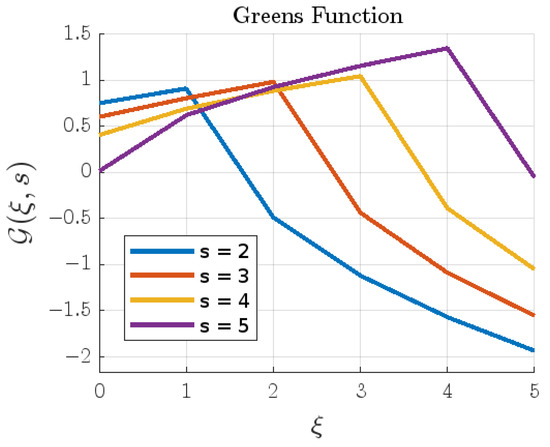
Let us consider

$$\left\{\begin{array}{c}\left({\nabla }_{\rho \left(0\right)}^{1.5}u\right)\left(\xi \right)+\xi u^2\left(\xi \right)=0,\xi \in {\mathbb{N}}_2^5,\hfill \\ u\left(0\right)+u\left(5\right)=0,\left(\nabla u\right)\left(1\right)+\left(\nabla u\right)\left(5\right)=0.\hfill \end{array}\right.$$

(15)

Here, $m=0$, $n=5$, $\nu =1.5$ and $\mathfrak{f}(\xi ,r)=\xi r^2$. In this case, the related Green’s function’s graph is plotted in Figure 1.

Clearly,

$$\left|\mathfrak{f}(\xi ,r)\right|\le {\mathfrak{p}}_{\mathfrak{1}}\left(\xi \right){\mathfrak{q}}_{\mathfrak{1}}\left(\left|r\right|\right),(\xi ,r)\in {\mathbb{N}}_2^5\times \mathbb{R},$$

where

$${\mathfrak{p}}_{\mathfrak{1}}\left(\xi \right)=\xi ,\xi \in {\mathbb{N}}_2^5$$

and

$${\mathfrak{q}}_{\mathfrak{1}}\left(\left|r\right|\right)={\left|r\right|}^2=r^2,r\in \mathbb{R}.$$

Also, ${\mathfrak{p}}_{\mathfrak{1}}:{\mathbb{N}}_2^5\to [0,\infty )$ and ${\mathfrak{q}}_{\mathfrak{1}}:[0,\infty )\to [0,\infty )$ is a nondecreasing function. As a result, one can easily verify that (C1) of Theorem 7 holds true. Moreover,

$${\Omega }_1=\underset{\xi \in {\mathbb{N}}_2^5}{max}{\mathfrak{p}}_{\mathfrak{1}}\left(\xi \right)=5.$$

Now, we calculate L. We have $\Lambda =-2.8846$. Then,

$$L\left(\xi \right)=\left(0.0788\right){\mathfrak{h}}_{0.5}(\xi ,\rho \left(0\right))+\left(0.3750\right){\mathfrak{h}}_{-0.5}(\xi ,\rho \left(0\right))+2.9459,\xi \in {\mathbb{N}}_0^5$$

and

$$L=\underset{t\in {\mathbb{N}}_0^5}{max}L\left(\xi \right)=3.3997.$$

There exists $0<N_1<0.05$ such that

$${\displaystyle \frac{N_1}{5\left(3.3997\right)N_1^2}}>1,$$

verifying (C2) of Theorem 7. Hence, from Theorem 7, it follows that (15) possesses a solution on ${\mathbb{N}}_0^5$.

Example 2.

Let us consider

$$\left\{\begin{array}{c}-\left({\nabla }_{\rho \left(0\right)}^{1.5}{u}_1\right)\left(\xi \right)=\xi +\left(0.1\right)sin{u}_2\left(\xi \right),\xi \in {\mathbb{N}}_2^5,\hfill \\ -\left({\nabla }_{\rho \left(m\right)}^{1.5}{u}_2\right)\left(\xi \right)=\xi +\left(0.1\right)cos{u}_1\left(\xi \right),\xi \in {\mathbb{N}}_2^5,\hfill \\ u_1\left(0\right)+u_1\left(5\right)=0,\left(\nabla u_1\right)\left(1\right)+\left(\nabla u_1\right)\left(5\right)=0,\hfill \\ u_2\left(0\right)+u_2\left(5\right)=0,\left(\nabla u_2\right)\left(1\right)+\left(\nabla u_2\right)\left(5\right)=0.\hfill \end{array}\right.$$

(16)

Here, $m=0$, $n=5$, $\nu =1.5$ and ${\mathfrak{f}}_{\mathfrak{1}}(\xi ,u_1\left(\xi \right),u_2\left(\xi \right))=\xi +\left(0.1\right)sin{u}_2\left(\xi \right)$, and ${\mathfrak{f}}_{\mathfrak{2}}(\xi ,u_1\left(\xi \right),u_2\left(\xi \right))=\xi +\left(0.1\right)cos{u}_1\left(\xi \right)$. Clearly,

$$\left|{\mathfrak{f}}_{\mathfrak{i}}\left(\xi ,v_1,v_2\right)-{\mathfrak{f}}_{\mathfrak{i}}\left(\xi ,w_1,w_2\right)\right|\le l_i\left|v_1-w_1\right|+m_i\left|v_2-w_2\right|,\mathrm{for}i=1,2$$

for each $t\in {\mathbb{N}}_2^5$ and all $\left(v_1,v_2\right)$, $\left(w_1,w_2\right)\in B\times B$ with $l_1=0$, $l_2=0.1$, $m_1=0.1$, $m_2=0$. We have $\Lambda =-2.8846$. Then,

$$L\left(\xi \right)=\left(0.0788\right){\mathfrak{h}}_{0.5}(\xi ,\rho \left(0\right))+\left(0.3750\right){\mathfrak{h}}_{-0.5}(\xi ,\rho \left(0\right))+2.9459,\xi \in {\mathbb{N}}_0^5$$

and

$$L=\underset{\xi \in {\mathbb{N}}_0^5}{max}L\left(\xi \right)=3.3997.$$

Since

$$\lambda =L\left(l_1+l_2\right)+L\left(m_1+m_2\right)=0.6799\in (0,1),$$

by Theorem 9, problem (16) has a unique solution in $\mathfrak{B}\times \mathfrak{B}$.

8. Conclusions

In this manuscript, we were able to deduce the exact expression of Green’s function related to the new one for an anti-periodic problem within the literature (1)–(2). We obtained an upper bound for its sum, and under some suitable conditions, we were able to prove existence and non-existence results, based on different fixed-point theorems. Then, we studied a system of two equations of the type studied above, and, again, we were able to deduce existence results. In the end, we were able to show the applicability of these theoretical findings with some particular examples. To our knowledge, this is the first research study in which such results have been established for this problem.

According to us, the above-mentioned results can be extended in some future works, where the authors may study different kind of systems. Moreover, using different methods, they may obtain different existence results.

References

- Miller, K.S.; Ross, B. Fractional Difference Calculus. Univalent Functions, Fractional Calculus, and Their Applications; Ellis Horwood Series in Mathematics and Its Applications; Horwood: Chichester, UK, 1989. [Google Scholar]
- Bohner, M.; Peterson, A. Dynamic Equations on Time Scales: An Introduction with Applications; Springer: Boston, MA, USA, 2001. [Google Scholar]
- Ferreira, R.A.C. Discrete Fractional Calculus and Fractional Difference Equations; Springer Briefs in Mathematics; Springer: Cham, Switzerland, 2022. [Google Scholar]
- Goodrich, C.; Peterson, A.C. Discrete Fractional Calculus; Springer: Cham, Switzerland, 2015. [Google Scholar]
- Atici, F.; Eloe, P. Discrete fractional calculus with the nabla operator. Elect. J. Qual. Theory Differ. Equ. 2009, 2009, 1–12. [Google Scholar] [CrossRef]
- Ahrendt, K.; Castle, L.; Holm, M.; Yochman, K. Laplace transforms for the nabla-difference operator and a fractional variation of parameters formula. Commun. Appl. Anal. 2012, 16, 317–348. [Google Scholar]
- Bastos, N.; Torres, D. Combined delta-nabla sum operator in discrete fractional caclulus. Commun. Frac. Calc. 2010, 41–47. [Google Scholar]
- Brackins, A. Boundary Value Problems of Nabla Fractional Difference Equations. Ph.D. Thesis, The University of Nebraska—Lincoln, Lincoln, NE, USA, 2014; 92p. [Google Scholar]
- Gholami, Y.; Ghanbari, K. Coupled systems of fractional ∇-difference boundary value problems. Differ. Equ. Appl. 2016, 8, 459–470. [Google Scholar] [CrossRef]
- Jonnalagadda, J.M. On two-point Riemann-Liouville type nabla fractional boundary value problems. Adv. Dyn. Syst. Appl. 2018, 13, 141–166. [Google Scholar]
- Li, Q.; Liu, Y.; Zhou, L. Fractional boundary value problem with nabla difference equation. J. Appl. Anal. Comput. 2021, 11, 911–919. [Google Scholar] [CrossRef] [PubMed]
- Liu, X.; Jia, B.; Gensler, S.; Erbe, L.; Peterson, A. Convergence of approximate solutions to nonlinear Caputo nabla fractional difference equations with boundary conditions. Electron. J. Differ. Equ. 2020, 2020, 1–19. [Google Scholar] [CrossRef]
- Chen, C.; Bohner, M.; Jia, B. Existence and uniqueness of solutions for nonlinear Caputo fractional difference equations. Turk. J. Math. 2020, 44, 857–869. [Google Scholar] [CrossRef]
- Goar, S.J. A Caputo Boundary Value Problem in Nabla Fractional Calculus. Ph.D. Thesis, The University of Nebraska—Lincoln, Lincoln, NE, USA, 2016. [Google Scholar]
- Ikram, A. Lyapunov inequalities for nabla Caputo boundary value problems. J. Differ. Equ. Appl. 2019, 25, 757–775. [Google Scholar] [CrossRef]
- Dimitrov, N.D.; Jonnalagadda, J.M. Existence of positive solutions for a class of nabla fractional boundary value problems. Fractal Fract. 2025, 9, 131. [Google Scholar] [CrossRef]
- Dimitrov, N.D.; Jonnalagadda, J.M. Existence, uniqueness and stability of solutions of a nabla fractional difference equations. Fractal Fract. 2024, 8, 591. [Google Scholar] [CrossRef]
- Cabada, A.; Dimitrov, N.; Jonnalagadda, J.M. Non-trivial solutions of non-autonomous nabla fractional difference boundary value problems. Symmetry 2021, 13, 1101. [Google Scholar] [CrossRef]
- Eralp, B.; Topal, F.S. Monotone method for discrete fractional boundary value problems. Int. J. Nonlinear Anal. Appl. 2022, 13, 1989–1997. [Google Scholar]
- Atici, F.M.; Eloe, P.W. Linear systems of fractional nabla difference equations. Rocky Mt. J. Math. 2011, 41, 353–370. [Google Scholar] [CrossRef]
- Wei, Y.; Chen, Y.; Liu, T.; Wang, Y. Lyapunov functions for nabla discrete fractional order systems. ISA Trans. 2019, 88, 82–90. [Google Scholar] [CrossRef] [PubMed]
- Chen, C.; Jia, B.; Liu, X.; Erbe, L. Existence and Uniqueness Theorem of the Solution to a Class of Nonlinear Nabla Fractional Difference System with a Time Delay. Mediterr. J. Math. 2018, 15, 212. [Google Scholar] [CrossRef]
- El-Sayed, A.M.A.; Abdurahman, M.; Fouad, H.A. Existence and stability results for the integrable solution of a singular stochastic fractional-order integral equation with delay. J. Math. Comput. Sci. 2024, 33, 17–26. [Google Scholar] [CrossRef]
- Luo, M.; Qiu, W.; Nikan, O.; Avazzadeh, Z. Second-order accurate, robust and efficient ADI Galerkin technique for the three-dimensional nonlocal heat model arising in viscoelasticity. Appl. Math. Comput. 2023, 440, 127655. [Google Scholar] [CrossRef]
- Agarwal, R.P.; Meehan, M.; O’Regan, D. Fixed Point Theory and Applications; Cambridge University Press: Cambridge, UK, 2001. [Google Scholar]
Disclaimer/Publisher’s Note: The statements, opinions and data contained in all publications are solely those of the individual author(s) and contributor(s) and not of MDPI and/or the editor(s). MDPI and/or the editor(s) disclaim responsibility for any injury to people or property resulting from any ideas, methods, instructions or products referred to in the content. |
© 2025 by the authors. Licensee MDPI, Basel, Switzerland. This article is an open access article distributed under the terms and conditions of the Creative Commons Attribution (CC BY) license (https://creativecommons.org/licenses/by/4.0/).