A Mathematical Survey of Image Deep Edge Detection Algorithms: From Convolution to Attention

Abstract

Edge detection, a cornerstone of computer vision, identifies intensity discontinuities in images, enabling applications from object recognition to autonomous navigation. This survey presents a mathematically grounded analysis of edge detection’s evolution, spanning traditional gradient-based methods, convolutional neural networks (CNNs), attention-driven architectures, transformer-backbone models, and generative paradigms. Beginning with Sobel and Canny’s kernel-based approaches, we trace the shift to data-driven CNNs like Holistically Nested Edge Detection (HED) and Bidirectional Cascade Network (BDCN), which leverage multi-scale supervision and achieve ODS (Optimal Dataset Scale) scores 0.788 and 0.806, respectively. Attention mechanisms, as in EdgeNAT (ODS 0.860) and RankED (ODS 0.824), enhance global context, while generative models like GED (ODS 0.870) achieve state-of-the-art precision via diffusion and GAN frameworks. Evaluated on BSDS500 and NYUDv2, these methods highlight a trajectory toward accuracy and robustness, yet challenges in efficiency, generalization, and multi-modal integration persist. By synthesizing mathematical formulations, performance metrics, and future directions, this survey equips researchers with a comprehensive understanding of edge detection’s past, present, and potential, bridging theoretical insights with practical advancements.

1. Introduction

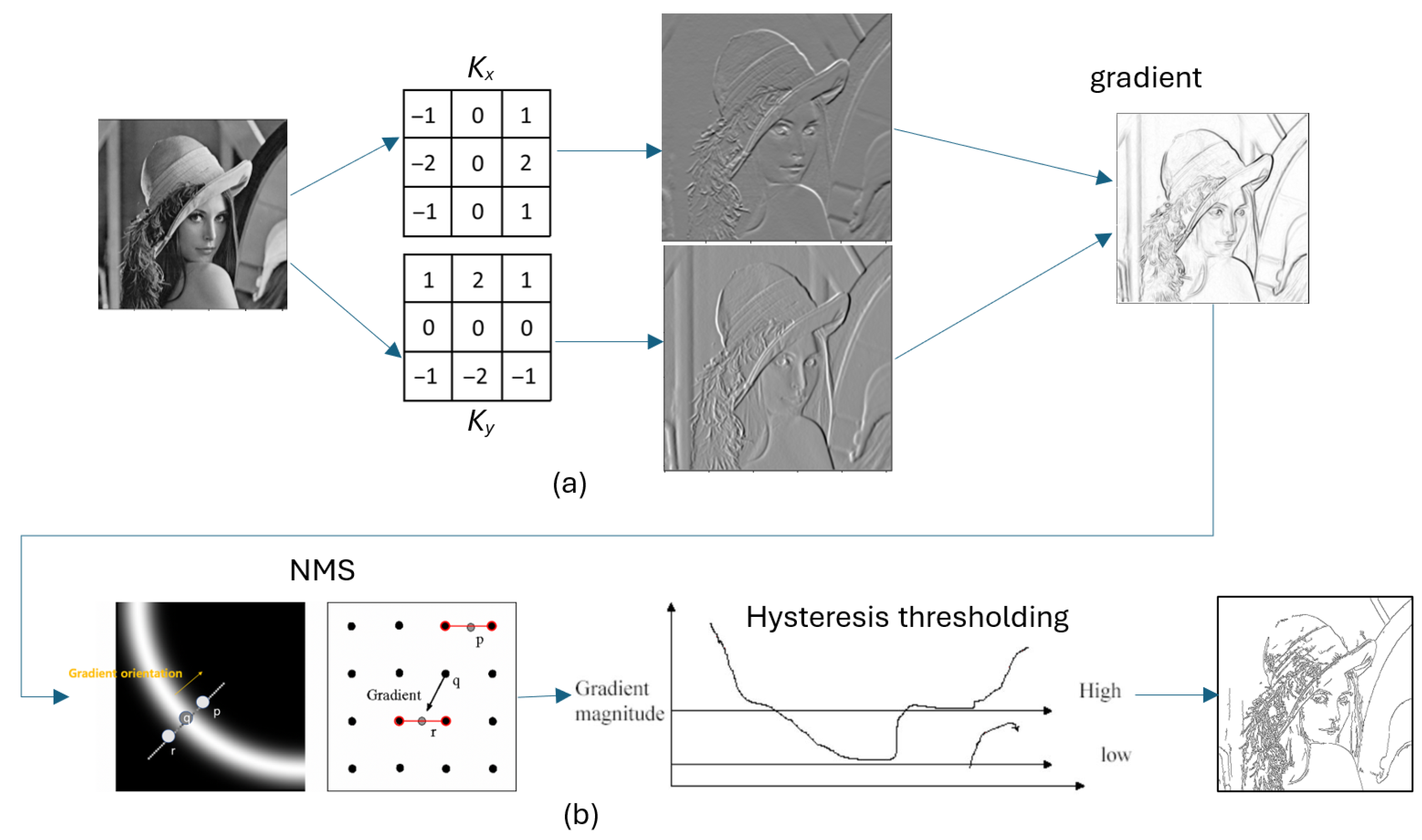
Edge detection, a cornerstone of computer vision, involves identifying boundaries within images where intensity changes abruptly. It serves as a fundamental preprocessing step for numerous downstream tasks, including object recognition, image segmentation, and autonomous navigation [1,2,3,4,5,6,7]. These edges, conveying essential structural and perceptual information, have been one of the central focuses of research in computer vision and image processing for decades, evolving from hand-crafted filters to sophisticated deep learning models. Early methods like Sobel [8], Canny [9] and others [10,11,12] relied on gradient-based operations, offering simplicity but struggling with noise and complex scenes. 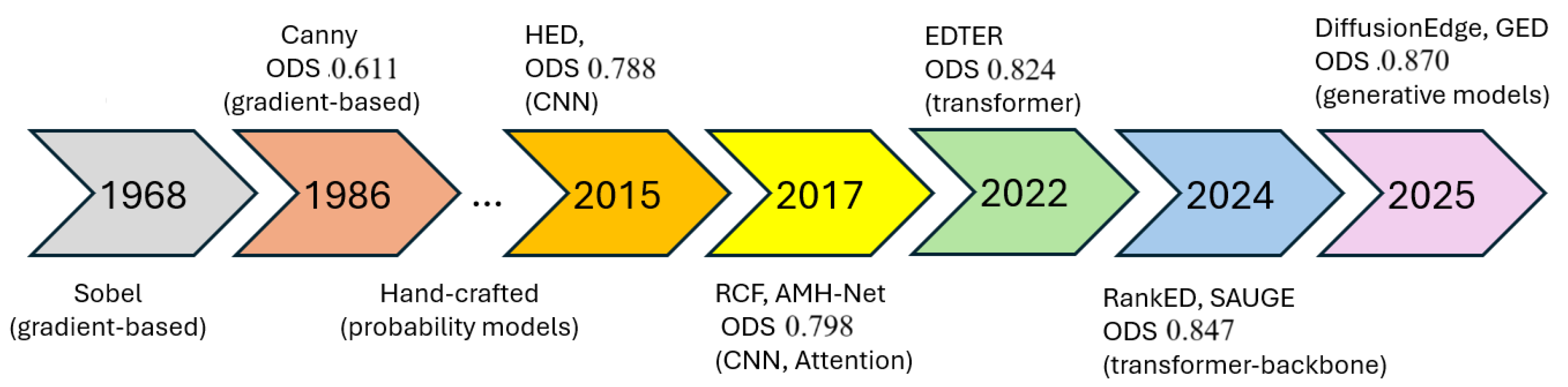The advent of convolutional neural networks (CNNs) marked a paradigm shift, introducing trainable feature extraction that significantly improved accuracy on benchmarks like BSDS500 [13]. More recently, attention mechanisms and generative approaches have pushed the frontier, achieving state-of-the-art performance by capturing global context and refining edge quality. Figure 1 shows the timeline of edge detection paradiams, from gadient-based methods to attention-based methods.

These advancements are driven by mathematical innovations such as transformer mechanisms (Equation (25)) and diffusion processes (Equation (51)). However, several key challenges remain unresolved, including computational inefficiency (e.g., the high complexity of transformers), limited generalization across datasets, insufficient multi-modal robustness, lack of theoretical clarity in parameter interpretation, and unstable training dynamics in generative models (Section 7).

While numerous surveys have reviewed edge detection methods, few provide a mathematically grounded perspective that unifies traditional, CNN-based, and emerging paradigms under a consistent analytical framework. Therefore, a survey that addresses these critical challenges through mathematical analysis is both timely and essential for advancing the real-world applicability of edge detection techniques.

This survey traces the evolution of edge detection. Besides the traditional gradient-based methods, it focuses on mainstream supervised deep learning methods for general edge detection, including CNN-based approaches, such as Holistically Nested Edge Detection (HED) [15], encoder–decoder (Bidirectional Cascade Network (BDCN) [16] and NHP [17]), attention-transformer-driven methods, including VST [18], EDTER [19], EdgeNAT [20], hybrid transformer-backbone (e.g., RankED [21] and SAUGE [22]), and generative algorithms (e.g., GED [14]), while excluding unsupervised, graph-based, reinforcement learning-based, and salient object detection methods due to their limited mathematical development or specific application focus.

Our objective is to provide a comprehensive, mathematically grounded analysis of these developments, synthesizing their strengths and limitations (Section 6) and identifying future directions (Section 7). Section 2 reviews Sobel and Canny, establishing the baseline. Section 3 examines early CNNs (HED [15], RCF [23]) and encoder–decoder innovations (BDCN [16], DexiNed [24], and NHP [17]), highlighting loss function designs and time efficiency. Section 4 explores attention-based and generative methods, from AMH-Net [25] to GED, emphasizing hybrid paradigms. Section 5 details the evaluation frameworks, while Section 6 compares all methods across accuracy and efficiency. Section 7 presents the current challenges and possible directions, and Section 8 concludes with reflections on the field’s trajectory.

2. Traditional Gradient-Based Edge Detection Methods

Before the advent of deep learning, edge detection relied on traditional methods rooted in mathematical operations on image gradients. These approaches, developed decades ago, remain foundational due to their simplicity and interpretability, though they lack the adaptability of modern techniques. This section examines two classic methods: the Sobel operator [8], introduced in 1968, and the Canny edge detector [9], proposed in 1986. Both are based on detecting intensity changes in an image I and have significantly influenced the development of subsequent techniques, laying the groundwork for the data-driven paradigms explored in Section 3.

2.1. Sobel Operator

The Sobel operator [8], developed by Irwin Sobel in 1968 as part of early computer vision research, is a lightweight method for approximating image gradients using convolution kernels. For a grayscale image $I(x,y)$, it computes the gradient components in the horizontal ($G_x$) and vertical ($G_y$) directions:

$$G_x=I\ast K_x,G_y=I\ast K_y,$$

(1)

where ∗ denotes convolution, and the kernels are

$$K_x=\left[\begin{array}{ccc}-1& 0& 1\\ -2& 0& 2\\ -1& 0& 1\end{array}\right],K_y=\left[\begin{array}{ccc}-1& -2& -1\\ 0& 0& 0\\ 1& 2& 1\end{array}\right].$$

(2)

The gradient magnitude, representing edge strength, is

$$|\nabla I|=\sqrt{G_x^2+G_y^2},$$

(3)

often approximated as $|G_x|+|G_y|$ for computational efficiency. A threshold T is applied to $|\nabla I|$ to produce a binary edge map $\widehat{y}$.

Sobel’s simplicity—requiring only small 3 × 3 kernels, has linear complexity, $O\left(hw\right)$, for image dimensions $h\times w$ but struggles with noise and complex scenes. Also, it lacks robustness to complex scenes. Its fixed kernels cannot adapt to varying edge characteristics, limiting its performance on datasets like BSDS500 [13], where no standard ODS F-score (Section 5.2) is typically reported due to its heuristic nature.

2.2. Canny Edge Detector

John Canny’s edge detector [9], introduced in 1986, builds on gradient-based methods like Sobel with a multi-stage pipeline to improve edge quality. It begins with noise reduction via Gaussian smoothing:

$$I_{\sigma }=I\ast G_{\sigma },G_{\sigma }(x,y)={\displaystyle \frac{1}{2\pi {\sigma }^2}}{e}^{-{\displaystyle \frac{x^2+y^2}{2{\sigma }^2}}},$$

(4)

where $G_{\sigma }$ is a Gaussian kernel with standard deviation $\sigma$. Gradient magnitude $|\nabla I_{\sigma }|$ and direction $\theta =arctan(G_y/G_x)$ are then computed, typically using Sobel kernels.

Canny introduces two key post-processing steps: non-maximum suppression (NMS) and hysteresis thresholding. NMS refines edge maps by thinning edges to a single pixel width, retaining only the local maxima in $|\nabla I_{\sigma }|$ along $\theta$, reducing false positives. Hysteresis uses two thresholds, $T_{\mathrm{low}}$ and $T_{\mathrm{high}}$, to classify strong edges ($|\nabla I_{\sigma }|>T_{\mathrm{high}}$) and connect weak edges ($T_{\mathrm{low}}<|\nabla I_{\sigma }|\le T_{\mathrm{high}}$) if adjacent to strong ones, yielding a binary edge map $\widehat{y}$.

Canny’s sophisticated approach offers improved noise robustness and edge continuity compared to the Sobel operator, but its reliance on hand-tuned parameters ($\sigma$, $T_{\mathrm{low}}$, $T_{\mathrm{high}}$) limits its adaptability to varying image conditions (see Figure 2).

Table 1. Comparison of traditional edge detection methods in Section 2. Both rely on gradient operations, with Canny enhancing Sobel via multi-stage processing, yet both lack the adaptability of deep learning approaches.

Method	Year	Key Operation	Limitations
Sobel [8]	1968	Gradient magnitude ($|\nabla I|$)	Noise-sensitive, non-adaptive
Canny [9]	1986	Gaussian + NMS + Hysteresis	Parameter-dependent, heuristic

summerizes their difference.

3. Convolutional Neural Networks for Edge Detection

The advent of deep learning marked a transformative shift in edge detection, replacing hand-crafted filters like Sobel [8] and Canny [9] with data-driven convolutional neural networks (CNNs). We examine the progression of CNN-based methods, which leverage hierarchical feature extraction to outperform traditional approaches on benchmarks like BSDS500 [13]. We divide this evolution into two phases: early CNN approaches, exemplified by Holistically Nested Edge Detection (HED) [15] and Richer Convolutional Features (RCFs) [23], and encoder–decoder innovations, represented by the Bidirectional Cascade Network (BDCN) [16] and Dense Extreme Inception Network (DexiNed) [24]. These methods laid the groundwork for the attention-based paradigms explored in Section 4, with their loss functions critical to optimizing edge predictions.

3.1. Early CNN Approaches

Convolutional operations are particularly effective for local feature extraction such as edges due to their inherent spatial locality and ability to capture intensity variations. A convolution layer applies a kernel $K\in {\mathbb{R}}^{k\times k}$ across an image $I\in {\mathbb{R}}^{h\times w}$, computing the local weighted sums at each location:

$$(I\ast K)(x,y)=\sum _{i=-r}^r\sum _{j=-r}^{r}K(i,j)·I(x+i,y+j),$$

(5)

where $r=\lfloor k/2\rfloor$. This operation aggregates pixel intensities in a local neighborhood, making it sensitive to spatial discontinuities in intensity, which are characteristic of edges. Classical edge detectors such as Sobel, Prewitt, and Roberts are special cases of fixed convolutional kernels designed to approximate gradients. In modern convolutional neural networks (CNNs), these filters are learned from data, and empirical evidence consistently shows that the first-layer filters resemble oriented edge detectors. This occurs because minimizing loss on visual tasks naturally encourages the network to detect strong local contrast patterns. Furthermore, convolution enforces translation invariance and parameter sharing, making it both efficient and robust for detecting edges regardless of their position in the image. Therefore, convolution serves as a mathematically grounded and empirically validated foundation for edge extraction in both classical and deep learning-based frameworks.

The initial application of CNNs to edge detection adapted pretrained networks like VGG-16 [26] to produce dense edge maps. Two representative approaches, HED and RCF, are described here, with HED introducing multi-scale supervision and RCF emphasizing feature richness, both employing loss functions that prioritize hierarchical learning.

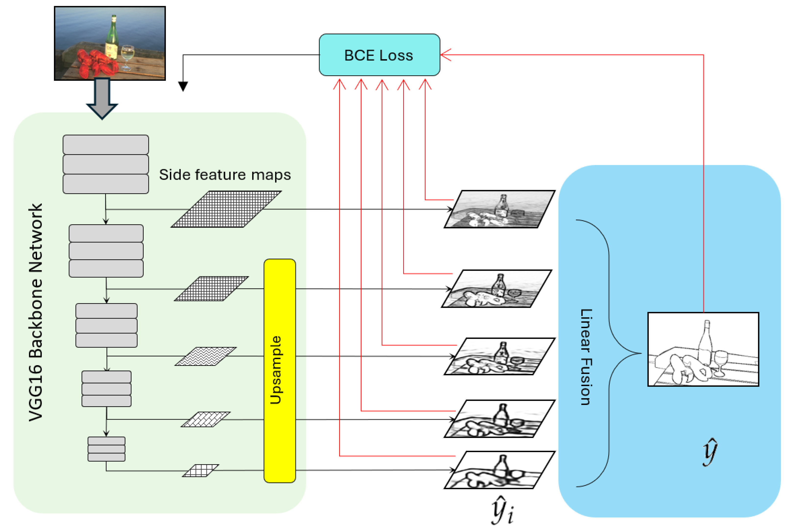
3.1.1. Holistically Nested Edge Detection (HED)

Proposed by Xie and Tu [15] in 2015, HED was among the first to apply CNNs holistically to edge detection, achieving an ODS F-score of 0.788 on BSDS500. HED modifies VGG16 by removing fully connected layers and extracting multi-scale feature maps $F_1,F_2,\dots ,F_5$ from its five blocks. Each block produces a side output via a 1 × 1 convolution followed by a sigmoid activation:

$${\widehat{y}}_i=\mathrm{sigmoid}\left({\mathrm{Conv}}_{1\times 1}\left(F_i\right)\right),$$

(6)

where $i=1,\dots ,5$, representing edge features at different scales—from local to global views. The side outputs are upsampled to the original image resolution, then fused by a weighted combination to produce the final edge map ($\widehat{y}$):

$$\widehat{y}=\mathrm{sigmoid}\left(\sum _{i=1}^5{w}_i{\widehat{y}}_i\right),$$

(7)

with $w_i$ as learned weights.

HED formulates edge detection as a per-pixel binary classification problem and employs a multi-scale, class-balanced binary cross-entropy (BCE) loss to supervise learning at different stages of the network. The total loss combines the losses from multiple side outputs and the final fused output, defined as

$$L_{\mathrm{HED}}=\sum _{m=1}^M{\alpha }_m·{\mathcal{L}}_{\mathrm{side}}^{\left(m\right)}+{\alpha }_f·{\mathcal{L}}_{\mathrm{fuse}},$$

(8)

where M is the number of side outputs, ${\mathcal{L}}_{\mathrm{side}}^{\left(m\right)}$ denotes the class-balanced BCE loss for the m-th side output, and ${\mathcal{L}}_{\mathrm{fuse}}$ is the loss for the final fused prediction. Each loss term is computed as

$$L_{\mathrm{BCE}}=-\beta \sum _{i\in Y_{+}}log\left({\widehat{y}}_i\right)-(1-\beta )\sum _{i\in Y_{-}}log(1-{\widehat{y}}_i),$$

(9)

where $Y_{+}$ and $Y_{-}$ represent the sets of edge and non-edge pixels, respectively, ${\widehat{y}}_i$ is the predicted edge probability at pixel i, and $\beta ={\displaystyle \frac{|Y_{-}|}{|Y_{+}|+|Y_{-}|}}$ balances the contributions of positive and negative samples. This loss formulation encourages the model to accurately predict edge pixels while addressing the severe class imbalance typical in edge detection tasks. This loss encourages fine local edges from lower layers (e.g., $F_1$) and object context from higher layers (e.g., $F_5$), outperforming traditional methods (see Figure 3).

3.1.2. Richer Convolutional Features (RCFs)

Liu et al. [23] extended HED at CVPR 2017 with RCF, improving the ODS F-score to 0.798 on BSDS500. RCF also uses VGG16 but aggregates intermediate features within each block $k=1,\dots ,5$:

$$F_k=\sum _j{\mathrm{Conv}}_{1\times 1}\left(F_{k,j}\right),$$

(10)

producing side outputs ${\widehat{y}}_k=\mathrm{sigmoid}\left({\mathrm{Conv}}_{1\times 1}\left(F_k\right)\right)$ and a fused output $\widehat{y}=\mathrm{sigmoid}\left({\sum }_{k=1}^5{w}_k{\widehat{y}}_k\right)$.

The RCF loss function mirrors that of HED, using the same BCE form (Equation (9)):

$$L_{\mathrm{RCF}}=L_{\mathrm{BCE}}(y,\widehat{y})+\sum _{k=1}^5{\alpha }_k{L}_{\mathrm{BCE}}(y,{\widehat{y}}_k),$$

(11)

differing only in the source of side outputs (richer intra-block features vs. the HED block endpoints). This similarity enhances details while maintaining multi-scale supervision (see Figure 3), achieving higher accuracy at ODS 0.798 on BSDS500 dataset.

Given an input image of size $h\times w\times c$, the time complexity per convolutional layer in early CNN-based edge detection methods, such as HED and RCF, is generally proportional to

$$O(h·w·k^2·c·c_{\mathrm{out}})$$

(12)

where h and w are the height and width of the input, c is the number of input channels, k is the kernel size, and $c_{\mathrm{out}}$ is the number of output channels. The total time complexity across all layers depends on the network’s depth and structure:

$$O\left(\sum _{\ell =1}^L{h}_{\ell }·w_{\ell }·k_{\ell }^2·c_{\ell }·c_{\ell ,\mathrm{out}}\right)$$

(13)

where L is the number of layers, and $h_{\ell }$, $w_{\ell }$, $c_{\ell }$, $c_{\ell ,\mathrm{out}}$, and $k_{\ell }$ represent the parameters of the ℓ-th layer. Since later layers often operate on downsampled feature maps, the actual complexity is lower than a linear multiple of input size. In practice, for architectures like HED or RCF using VGG-style backbones (e.g., $L=16$, $k=3$), the overall complexity can be approximated by

$$O(L·h·w·c)$$

(14)

assuming fixed small kernels and proportional input/output channels per layer.

3.2. Encoder–Decoder Innovations

Encoder–decoder architectures have become pivotal for edge detection, addressing the resolution and continuity limitations of early CNNs. The encoder downsamples an input image I into compact feature maps $F_1,\dots ,F_n$, capturing multi-scale features from local textures to global semantics. The decoder upsamples these, often with skip connections, to produce high-resolution edge maps $\widehat{y}$, ensuring precise boundary localization. This paradigm excels in edge detection by balancing fine details with contextual understanding. Notably, early CNNs like HED and RCF (Section 3.1) exhibit an encoder–decoder-like structure: their VGG16 backbones downsample features, and upsampling occurs in fusion layers. However, they lack explicit decoder modules, relying on side outputs, upsampling, and simple linear fusion, unlike formal encoder–decoder designs. This survey is, to our knowledge, the first to frame HED and RCF in this light, revealing a precursor to the innovations in the Bidirectional Cascade Network (BDCN) [16], Dense Extreme Inception Network (DexiNed) [24], and Normalized Hadamard Product (NHP) [17] fusion, which introduce specialized modules for a robust encoder–decoder flavor.

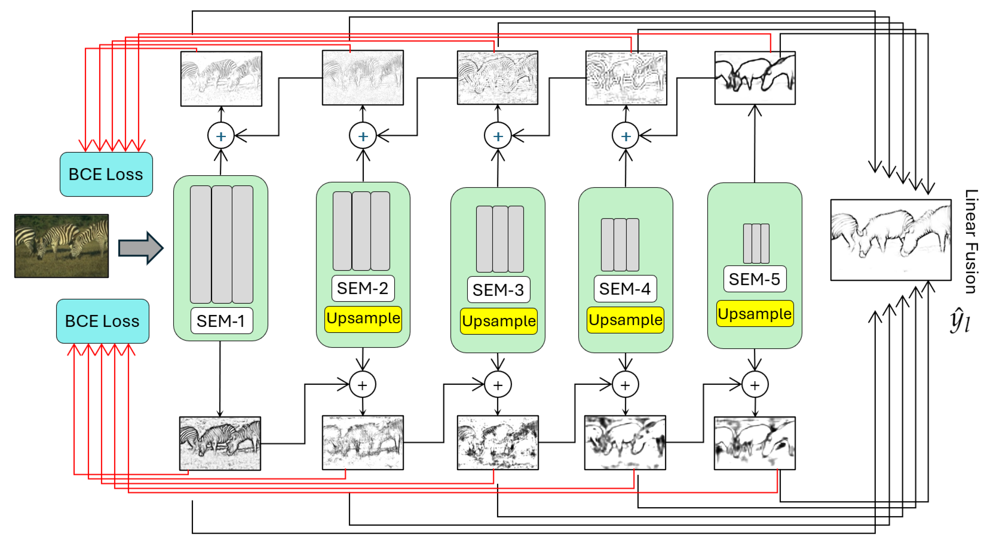
3.2.1. Bidirectional Cascade Network (BDCN)

He et al. [16] introduced BDCN at CVPR 2019, achieving an ODS F-score of 0.828 on BSDS500. BDCN formalizes the encoder–decoder paradigm, using a VGG16 encoder with a Scale Enhancement Module (SEM) to refine features $F_1,\dots ,F_5$. The SEM processes each feature map:

$$F_l^{\mathrm{SEM}}=\mathrm{ReLU}\left(\mathrm{BN}\left({\mathrm{Conv}}_{3\times 3}\left(F_l\right)\right)\right),$$

(15)

enhancing scale-specific edge details. These are upsampled by a decoder except $F_1^{\mathrm{SEM}}$, where a bidirectional cascade combines outputs across scales:

$$C_l={\mathrm{Conv}}_{1\times 1}\left(\mathrm{Concat}(U_l,C_{l+1}^{\mathrm{down}},C_{l-1}^{\mathrm{up}})\right),$$

(16)

where $U_l=\mathrm{Upsample}\left(F_l^{\mathrm{SEM}}\right)$, and $C_{l+1}^{\mathrm{down}}$, $C_{l-1}^{\mathrm{up}}$ are downward and upward cascade outputs. The edge map is ${\widehat{y}}_l=\mathrm{sigmoid}\left({\mathrm{Conv}}_{1\times 1}\left(C_l\right)\right)$, refining localization (see Figure 4).

The BDCN loss uses scale-specific BCE:

$$L_l=-\sum [y_{l}log\left({\widehat{y}}_l\right)+(1-y_l)log(1-{\widehat{y}}_l)],$$

(17)

with total loss

$$L_{\mathrm{BDCN}}=\sum _{l=1}^L{L}_l,$$

(18)

optimizing each layer’s ground truth $y_l$. This leverages the cascade’s decoding for precise edges.

3.2.2. Dense Extreme Inception Network (DexiNed)

Xavier et al. [24] presented DexiNed in 2020, achieving an ODS F-score of 0.729 on BSDS500. DexiNed uses an Xception-inspired encoder for features $F_1,\dots ,F_6$, upsampled in a dense decoder:

$$F_{l,\mathrm{up}}=\mathrm{interp}\left(F_l\right),$$

(19)

fused as $F_{\mathrm{fused}}=\mathrm{Concat}(F_{1,\mathrm{up}},\dots ,F_{6,\mathrm{up}})$, with outputs ${\widehat{y}}_l$ and $\widehat{y}$. Its BCE loss mirrors HED/RCF, enhancing edge continuity via dense fusion.

Recent work by Hu et al. [17] introduces normalized Hadamard product (NHP) fusion, achieving ODS 0.818 on BSDS500. NHP multiplies normalized VGG16 side outputs:

$$\mathrm{MASE}=\prod _i\mathrm{normalize}\left({\widehat{y}}_i\right),$$

(20)

producing Mutually Agreed Salient Edge (MASE) maps, refining edges. Like the BDCN cascade, the NHP operator formalizes the encoder–decoder flavor, surpassing HED/RCF.

3.3. Multi-Scale Feature Fusion in Edge Detection

The fusion process plays a vital role in CNN-based edge detection. Features extracted at multiple scales can effectively capture edges of varying thicknesses and complexities. Formally, let $F^{\left(m\right)}(x,y)$ denote the feature map or edge prediction at scale m for pixel location $(x,y)$, where $m=1,2,\dots ,M$ indexes the scales from fine to coarse. A common approach to fuse these multi-scale features is a weighted summation:

$$F_{\mathrm{fused}}(x,y)=\sum _{m=1}^M{\alpha }_m·F^{\left(m\right)}(x,y),$$

(21)

where ${\alpha }_m$ are learnable or fixed weights that control the contribution of each scale.

Alternatively, concatenation followed by a convolutional layer can be used:

$$F_{\mathrm{fused}}=\sigma \left(W\ast \mathrm{concat}(F^{\left(1\right)},F^{\left(2\right)},\dots ,F^{\left(M\right)})+b\right),$$

(22)

where W and b are the convolutional weights and bias, and $\sigma$ is a nonlinear activation function (e.g., ReLU or sigmoid).

The fusion of multi-scale features offers several theoretical benefits for edge detection. Fine-scale features extracted from early layers, excel at capturing thin, localized edges. In contrast, coarse-scale features from deeper layers have larger receptive fields, able to capture thicker boundaries and broader contextual patterns. By combining these complementary representations, the model becomes capable of detecting edges across a wide range of spatial scales and complexities. Additionally, this fusion improves robustness by mitigating the effects of noise in fine scales and compensating for missing details in coarser scales. As a result, multi-scale fusion enhances both the precision and completeness of edge predictions.

For example, consider three scales with predicted edge probabilities at pixel $(x,y)$: $F^{\left(1\right)}=0.9,F^{\left(2\right)}=0.6,F^{\left(3\right)}=0.3,$ and corresponding fusion weights: ${\alpha }_1=0.5,$ ${\alpha }_2=0.3, {\alpha }_3=0.2.$

The fused prediction at this pixel is

$$F_{\mathrm{fused}}=0.5\times 0.9+0.3\times 0.6+0.2\times 0.3=0.45+0.18+0.06=0.69.$$

This fusion combines strong fine-scale evidence with supporting coarser-scale information, yielding a more reliable edge prediction.

3.4. Effectiveness and Efficiency of CNN-Based Approaches

Table 2. Comparison of CNN-based edge detection methods. ODS reflects BSDS500 performance; key loss features highlight similarities and differences.

Method	Year	Venue	ODS (BSDS500)	Key Loss Feature
HED [15]	2015	ICCV	0.788	BCE, 5 side outputs + fusion
RCF [23]	2017	CVPR	0.798	BCE, 5 richer side outputs + fusion
BDCN [16]	2019	CVPR	0.806	BCE, scale-specific layers
DexiNed [24]	2020	arXiv	0.729	BCE, 6 side outputs + dense fusion
NHP [17]	2024	J. Imaging	0.818	BCE, NHP fusion + MASE maps

summarizes the CNN-based edge detection methods. Despite advances, CNN-based approaches face limitations. Their convolutional layers, constrained by fixed receptive fields, struggle to capture long-range dependencies essential for complex boundaries in datasets like BSDS500 [13]. Simple fusion in HED and RCF risks diluting fine edges, while encoder–decoder-based approaches introduce sophisticated fusion components (BDCN cascade and NHP fusion) for higher ODS.

Theoretically, the time complexity of encoder–decoder-based approaches remains in the same order as HED and RCF, $O(L·h·w·c)$, which is primarily based on convolutional backbones. However, due to its deeper supervision and multi-path design, these methods incur higher practical computational cost and memory usage compared to HED and RCF, limiting real-time use.

Moreover, CNN-based methods lack dynamic feature weighting, reducing adaptability to diverse edge patterns. Attention mechanisms address these challenges by capturing global context and prioritizing salient features, marking a significant evolution in edge detection.

4. Attention Mechanisms and Emerging Trends

The transition from CNN-based methods (Section 3) to attention-driven and generative paradigms marks a pivotal evolution in edge detection, emphasizing global context modeling and computational efficiency. While CNN-based and encoder–decoder approaches excel in hierarchical feature extraction and resolution recovery, they often struggle with capturing long-range dependencies due to their limited receptive fields. In contrast, attention mechanisms dynamically prioritize salient features across the entire image, overcoming the spatial limitations of conventional convolutional architectures (Section 3.2). These mechanisms enhance edge detection by being integrated into—or fully replacing—decoder components. This section highlights this natural progression, examining representative models such as AMH-Net [25], VST [18], EDTER [19], and EdgeNAT [20].

4.1. Attention-Based Contour Detection (AMH-Net)

AMH-Net [25] introduces a hybrid CNN–attention approach with an encoder–decoder flavor, using a ResNet-50 [27] encoder to extract multi-scale features $F_1,\dots ,F_n$ and an attention-gated CRF (AG-CRF) decoder to weight contour-relevant regions.

Unlike HED uniform fusion, AMH-Net introduces a two-stage fusion strategy. First, it uses AG-CRFs to refine and align features across scales by explicitly modeling contextual dependencies between different levels of abstraction. These AG-CRFs are enhanced with attention gates that dynamically weigh feature importance based on the current input, allowing the model to emphasize more informative contours and suppress irrelevant textures. In the second stage, the fused features are passed through additional convolutional layers to generate the final edge map. Equations (23) and (24) show its summarized formula:

$$M_{ij}=\mathrm{softmax}(W·[F_i,F_j]),$$

(23)

where W is a learned weight matrix, and $[F_i,F_j]$ denotes the concatenated features at positions i and j. The attention-gated output refines each feature map:

$$F_{i,\mathrm{refined}}=F_i+\sum _j{M}_{ij}{F}_j,$$

(24)

which is then integrated into a CRF framework for contour prediction. The CRF optimizes the edge map $\widehat{y}$ by minimizing an energy function combining unary and pairwise potentials, trained end-to-end with a cross-entropy loss akin to Equation (9).

This hierarchical and attention-driven fusion enables AMH-Net to produce more accurate and coherent edges, especially in cluttered or low-contrast regions. AMH-Net’s AG-CRFs module with attention mechanism improves localization over CNN-only methods like HED [15] and RCF [23], demonstrates strong performance on standard edge detection benchmarks such as BSDS500 and NYUDv2 over earlier methods like HED and RCF in both precision and robustness, foreshadowing the shift to global attention in later models. Its reliance on a CNN backbone limits its scope compared to pure transformer approaches, but it marks a critical step in the evolution from convolution to attention.

4.2. Transformer-Based Edge Detection

The transformer-based attention mechanism [28] was originally developed for natural language processing (NLP) but was later introduced to computer vision with the Vision Transformer (ViT) architecture [29]. Its core component, the scaled dot-product attention, allows models to dynamically prioritize salient regions across the input feature map $X\in {\mathbb{R}}^{N\times C}$, and is defined as

$$\mathrm{Attention}(Q,K,V)=\mathrm{Softmax}\left({\displaystyle \frac{Q{K}^T}{\sqrt{d_k}}}\right)V,$$

(25)

where $Q=X{W}_Q$, $K=X{W}_K$, and $V=X{W}_V$ are query, key, and value projections, and $d_k$ scales the dot product. This mechanism overcomes the fixed receptive field of convolutional operations, enabling the more effective modeling of long-range dependencies—a key advantage in vision tasks such as edge detection.

Among transformer-based vision models, the Vision Saliency Transformer (VST) [18], introduced at ICCV 2021, is notable for its ability to produce plausible object contours. VST is a transformer-based framework for salient object detection that explicitly incorporates boundary prediction as a complementary task. Built on a ViT-style encoder–decoder architecture, VST adopts a multi-task design in which saliency and boundary-specific tokens are decoded in parallel through a shared transformer decoder. This allows the model to simultaneously generate both a saliency map and a boundary map. The boundary prediction head is supervised using object contour annotations, enabling the network to learn spatially precise and semantically meaningful edges around salient regions. While VST is not intended as a general-purpose edge detector, its boundary outputs effectively highlight prominent object contours, particularly in cluttered or low-contrast scenes—achieving an S-measure of 0.91 on DUTS [30]. These saliency-aligned edge maps can be regarded as edge detection byproducts, especially valuable in applications focused on foreground object structure. However, they are not optimized for capturing background textures, fine-grained detail, or non-salient edges. Nonetheless, VST serves as a compelling example of how edge information can be jointly learned with saliency within a unified transformer-based framework.

Edge Detection with Transformer (EDTER) [19] (ECCV 2022) focuses on lightweight edge detection, achieving ODS 0.824 at 10 FPS on a Titan X. By integrating a CNN encoder with lightweight transformer layers, EDTER leverages a streamlined version of self-attention (Equation (25)) to refine edges efficiently. Its dual-task design, simultaneously optimizing edge detection and boundary refinement, enhances precision over DexiNed [24], though it struggles with severe class imbalance, addressed by later methods like RankED [21].

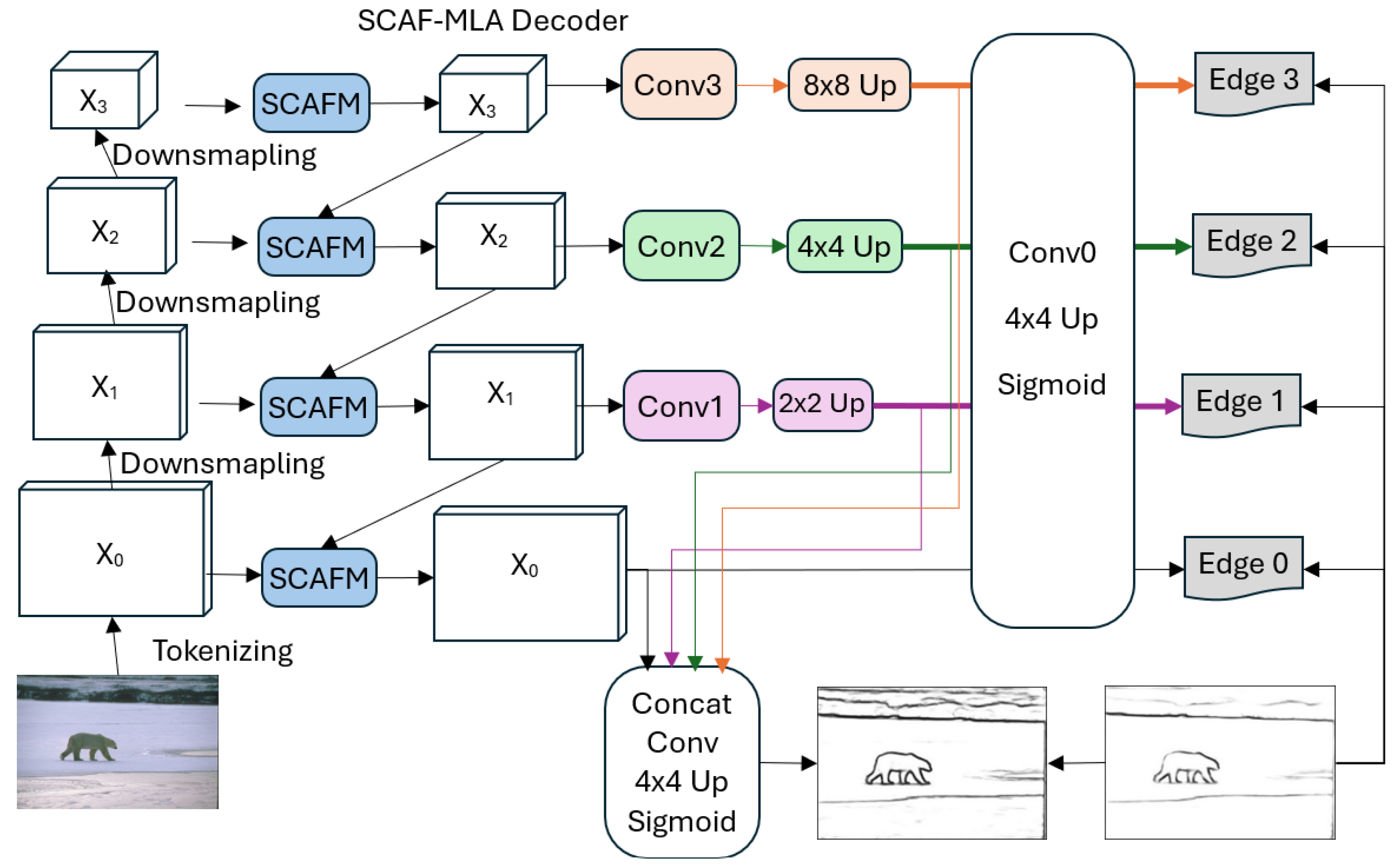
EdgeNAT [20] integrates a VGG16 encoder with a Dilated Attention Module, and introduces Scale-Adaptive Feature Multi-Level Aggregation (SCAF-MLA) as a decoder (see Figure 5). Its attention module follows Equation (25), while decoder SCAF-MLA is formalized as

$$\mathrm{SCAF}\text{-}\mathrm{MLA}=\sum _{i=1}^N{\beta }_i·\mathrm{Attention}(Q_i,K_i,V_i),$$

(26)

where ${\beta }_i$ weights multi-level features. Achieving ODS 0.860 and 12.5 FPS on BSDS500, EdgeNAT combines CNN and transformer features to enhance efficiency, surpassing the BDCN cascade (Equation (16)). Its multi-level focus improves edge continuity but struggles with severe class imbalance.

Transformer-based methods have collectively advanced the field of edge detection by demonstrating the power and effectiveness of attention mechanisms in capturing the global context. Given an input image of size $h\times w$ and a patch size of $p\times p$, the image is divided into non-overlapping patches, resulting in

$$n={\displaystyle \frac{h·w}{p^2}}$$

(27)

where n is the number of input tokens (patches), h and w are the height and width of the input image, and p is the height and width of each square patch. These approaches utilize the scaled dot-product attention mechanism, defined over the space ${\mathbb{R}}^{n\times d}$, where d is the feature dimension of the key vectors and n is the number of image patches. The computational complexity of the attention operation is $O\left(n^{2}d\right)$, stemming from the pairwise interactions among all elements in the sequence. Substituting $n=hw/p^2$, the complexity becomes

$$O\left({\displaystyle \frac{h^2{w}^{2}d}{p^4}}\right)$$

(28)

which reveals the quadratic dependence on image resolution. When the patch size p is fixed (as is common in practice), this can be approximated as

$$O\left(h^2{w}^{2}d\right)$$

(29)

where $d=768$∼1280, highlighting the substantial computational cost associated with applying full attention to high-resolution inputs as analyzed in Section 6.

Compared to non-transformer-based methods, transformer-based edge detection models tend to be more computationally intensive due to the self-attention mechanism, which scales quadratically with the number of input tokens.

4.3. Transformer-Backbone Edge Detection

Recently, with the rising power of transformer models, the trend in edge detection has shifted away from traditional backbones like VGG or ResNet. From 2023 to 2025, transformer-based backbones have dominated the field, with methods such as RankED [21] and SAUGE [22] leveraging pretraining to achieve ODS scores above 0.824. Unlike architecture-focused approaches like EDTER [19] or EdgeNAT [20], these methods emphasize non-transformer innovations—such as ranking-based and sorting losses or uncertainty modeling—highlighting how transformer backbones can amplify algorithmic advancements.

RankED (CVPR 2024) employs a Swin Transformer backbone [31] (Swin-B, ∼88 M parameters) to achieve ODS 0.824 on BSDS500, excelling in average precision (AP). Swin-B, pretrained on ImageNet-22K, processes 320 × 320 inputs through four hierarchical stages (patch size 4 × 4, feature dimensions 128 to 1024) using shifted window self-attention (Equation (25)). A lightweight convolutional decoder fuses multi-scale features, guided by a combined rank and sort loss:

$$\begin{array}{cc}\hfill L_{\mathrm{rank}}& ={\displaystyle \frac{1}{\left|P\right|}}\sum _{i\in P}\sum _{j\in N}{\displaystyle \frac{H(p_j-p_i)}{{\sum }_{k\in P\cup N}H(p_k-p_i)}},\hfill \end{array}$$

(30)

$$\begin{array}{cc}\hfill H\left(x\right)& =\left\{\begin{array}{cc}0\hfill & x<-ϵ\hfill \\ {\displaystyle \frac{x}{2ϵ}}+0.5\hfill & -ϵ\le x\le ϵ\hfill \\ 1\hfill & x>ϵ\hfill \end{array}\right.,\hfill \end{array}$$

(31)

$$\begin{array}{cc}\hfill L_{\mathrm{sort}}& ={\displaystyle \frac{1}{\left|P\right|}}\sum _{i\in P}\left({\Delta }_{\mathrm{sort}}\left(i\right)-{\Delta }_{\mathrm{sort}}^{\ast }\left(i\right)\right),\hfill \end{array}$$

(32)

$$\begin{array}{cc}\hfill {\Delta }_{\mathrm{sort}}\left(i\right)& ={\displaystyle \frac{1}{{\sum }_{j\in P}H(p_j-p_i)}}\sum _{j\in P}H(p_j-p_i)(1-c_j),\hfill \end{array}$$

(33)

$$\begin{array}{cc}\hfill {\Delta }_{\mathrm{sort}}^{\ast }\left(i\right)& ={\displaystyle \frac{{\sum }_{j\in P}H(p_j-p_i)[c_j>c_i](1-c_j)}{{\sum }_{j\in P}H(p_j-p_i)[c_j>c_i]}},\hfill \end{array}$$

(34)

$$\begin{array}{cc}\hfill L& =L_{\mathrm{rank}}+\alpha L_{\mathrm{sort}},\hfill \end{array}$$

(35)

where $P,N$ are edge and non-edge pixel sets, $p_i$ are predicted scores, and $c_i\in [0,1]$ are ground-truth certainty scores, computed as

$$c_i={\displaystyle \frac{1}{K}}\sum _{\ell =1}^{K}1[\exists p\in \mathrm{vicinity}\mathrm{of}i:y_{\ell ,p}=1],$$

with K annotators and $y_{\ell ,p}$ indicating edge labels in pixel i’s neighborhood. $H\left(x\right)$ is a smooth step function with threshold $ϵ$, $[c_j>c_i]$ is 1 if $c_j>c_i$ else 0, and $\alpha$ is a weighting factor (e.g., 0.5, or 0 if only one annotation exists)⁴ Certainty computation inferred from BSDS500; $\alpha =1$ assumed based on typical loss weighting; $ϵ$ and sampling strategy unavailable [21]. The rank loss optimizes AP, ranking edge pixels above non-edges to address class imbalance, while the sort loss aligns edge predictions with annotator certainty, tackling label uncertainty. Pairs are randomly sampled to reduce computational cost. RankED achieves robust boundaries in Multicue and NYUDv2, though high GPU memory demands limit efficiency compared to the EDTER transformer layers.

SAUGE (AAAI 2025) adapts the Segment Anything Model’s Vision Transformer [32] (SAM-ViT, likely ViT-H, ∼632 M parameters) for edge detection, achieving ODS 0.847 per AAAI 2025 [22]. SAM-ViT, pretrained on SA-1B (1B masks, 11 M images), processes 320 × 320 inputs as 16 × 16 patches, producing 64 × 64 × 1280 embeddings via 32 transformer layers. Unlike the SAM prompt-driven segmentation, SAUGE uses only the image encoder, bypassing the prompt encoder. A lightweight decoder (∼1.5% parameters, ∼9.5 M) fuses multi-granularity features, regressing edges aligned with human label uncertainty (see Figure 6). The loss comprises

$$\begin{array}{cc}\hfill L_{\mathrm{side}}^k& =-{\displaystyle \frac{1}{N}}\sum _i\left[w_i\left(y_i^{k}log{p}_i^k+(1-y_i^k)log(1-p_i^k)\right)\right],\hfill \end{array}$$

(36)

$$\begin{array}{cc}\hfill L_{\mathrm{diversity}}& ={\displaystyle \frac{1}{M}}\sum _{(m,n)\in \mathcal{C}}\left|\mathrm{XOR}(p^m,p^n)\right|,\hfill \end{array}$$

(37)

$$\begin{array}{cc}\hfill L_{\mathrm{guide}}& =-{\displaystyle \frac{1}{N}}\sum _i\left[c_i\left(y_i^{\mathrm{sobel}}log{p}_i+(1-y_i^{\mathrm{sobel}})log(1-p_i)\right)\right],\hfill \end{array}$$

(38)

$$\begin{array}{cc}\hfill L& =\sum _k{L}_{\mathrm{side}}^k+{\lambda }_{\mathrm{diversity}}{L}_{\mathrm{diversity}}+{\lambda }_{\mathrm{guide}}{L}_{\mathrm{guide}},\hfill \end{array}$$

(39)

where $L_{\mathrm{side}}^k$ supervises the side outputs (coarse, medium, fine) with pseudo-labels $y_i^k$ and weights $w_i$; $L_{\mathrm{diversity}}$ enforces distinct side predictions; $L_{\mathrm{guide}}$ aligns the final edges with the SAM Sobel maps using confidence weights $c_i$; and ${\lambda }_{\mathrm{diversity}}, {\lambda }_{\mathrm{guide}}$ are fixed constants. This loss ensures uncertainty alignment, generalizing across Multicue and NYUDv2, outperforming HED. The SAUGE SAM-driven approach contrasts RankED’s rank and sort innovation, marking a novel 2025 paradigm.

By leveraging transformer backbones, both RankED and SAUGE incur a minimum computational complexity of $O\left(h^2{w}^{2}d\right)$ (Equation (29)) due to the self-attention mechanism. As hybrid architectures, they combine convolutional feature extractors with transformer-based attention modules to balance local inductive bias and global context modeling. However, this integration significantly increases the actual computational cost, which limits their efficiency in practice (Section 6).

4.4. Generative Models for Edge Detection

In recent years, generative models—especially diffusion-based methods and adversarial frameworks—have emerged as powerful tools for edge detection. Unlike traditional discriminative models that directly predict binary edge maps from input images, generative approaches learn to synthesize edge structures, often modeling uncertainty and fine-grained detail more effectively. Two prominent examples are DiffusionEdge and GED (Generative Edge Detection).

DiffusionEdge (AAAI 2024) [33] applies a diffusion probabilistic model (DPM) [34] in latent space, achieving ODS 0.834 on BSDS500. The forward process adds noise over T steps:

$$q\left(x_t\right|x_{t-1})=\mathcal{N}(x_t;\sqrt{1-{\beta }_t}{x}_{t-1},{\beta }_{t}I),$$

(40)

enabling denoising via

$$p_{\theta }\left(x_{t-1}\right|x_t)=\mathcal{N}(x_{t-1};{\mu }_{\theta }(x_t,t),{\Sigma }_{\theta }(x_t,t)).$$

(41)

It uses a CNN-based encoder–decoder (∼200 M parameters) trained with uncertainty-aware cross-entropy:

$$L_{\mathrm{DiffusionEdge}}=-\sum _i\left[c_{i}log{p}_i+(1-c_i)log(1-p_i)\right].$$

(42)

Trained on BSDS500’s 200 images with augmentation for <30 epochs, it generalizes to BIPED, leveraging uncertainty distillation for ambiguous edges.

In contrast, Generative Edge Detection (GED) [14] leverages the pretrained Stable Diffusion backbone (∼116 M parameters), repurposing its U-Net-like encoder–decoder architecture within a conditional GAN (cGAN) [35,36] framework for latent-to-latent edge prediction. Instead of generating full-resolution RGB images, GED operates directly in the latent space, predicting edge maps from noisy latent representations of the input image. This design enables more efficient and semantically meaningful edge generation. A key contribution of GED is its ability to generate edge maps at multiple levels of granularity, controlled through a conditioning mechanism:

$$L_{\mathrm{GED}}={\displaystyle \frac{1}{N}}\sum _i|p_i-y_i|+{\lambda }_g\sum _i\left|g_i-g_i^{\ast }\right|,$$

(43)

where $g_i\in [0,1]$ is a side output controlling edge thickness (e.g., 0 for thin, 1 for thick)⁵ ${\lambda }_g\approx 0.1$ assumed for granularity balance; exact value unavailable [14]. Its single-step inference enhances efficiency, doubling DiffusionEdge’s throughput, and supports applications like medical imaging. GED achieves ODS 0.870, OIS 0.880, and AP 0.934 on BSDS500. It demonstrates how high-level generative modeling can be repurposed for fine-grained, structure-aware prediction tasks.

Diffusion-based edge detection models typically operate over multiple iterative steps to refine predictions. The overall computational complexity can be approximated as $O(T·L·h·w·c)$, where T is the number of diffusion steps (e.g., 1000). Each step generally involves a forward pass through a deep neural network, making diffusion models more computationally intensive than feedforward approaches.

Table 3. Comparison of Generative Edge Detection models.

Model	Type	Backbone	Notable Features	Output Characteristics
DiffusionEdge [33]	Latent diffusion	Custom denoising network (∼200 M)	Frequency-aware filtering, uncertainty distillation	Crisp, high-confidence edges
GED [14]	Finetuned Stable Diffusion	Stable Diffusion U-Net (∼116 M)	Latent-to-latent mapping, granularity control	Flexible, multi-scale edge maps

summarizes the differences between the two generative models.

5. Datasets and Evaluation Metrics

The evaluation of edge detection algorithms, from traditional methods (Section 2) to deep learning approaches (Section 3 and Section 4), relies on standardized datasets and metrics. This section reviews two pivotal datasets—BSDS500 [13] and NYUDv2 [37]—and key evaluation metrics, including the Optimal Dataset Scale (ODS) F-score and Optimal Image Scale (OIS) F-score. These tools provide a quantitative basis for comparing methods like HED (ODS 0.782) to SAUGE (ODS 0.860), highlighting advancements in accuracy and efficiency.

5.1. Datasets

The Berkeley Segmentation Dataset and Benchmark (BSDS500), introduced by Arbelaez et al. [13] in 2011, is the de facto standard for edge detection evaluation. It comprises 500 natural images (200 train, 100 validation, 100 test), each of size 481 × 321 pixels, with human-annotated ground truth edge maps y. Each image has multiple annotations (typically 5–7), reflecting subjective edge interpretations, averaged into a consensus map:

$$y(x,y)={\displaystyle \frac{1}{N}}\sum _{n=1}^N{y}_n(x,y),$$

(44)

where $y_n$ is the n-th annotator’s binary edge map, and N is the number of annotators. BSDS500’s diversity—spanning objects, textures, and scenes—challenges algorithms to detect perceptually significant edges, making it ideal for benchmarking methods.

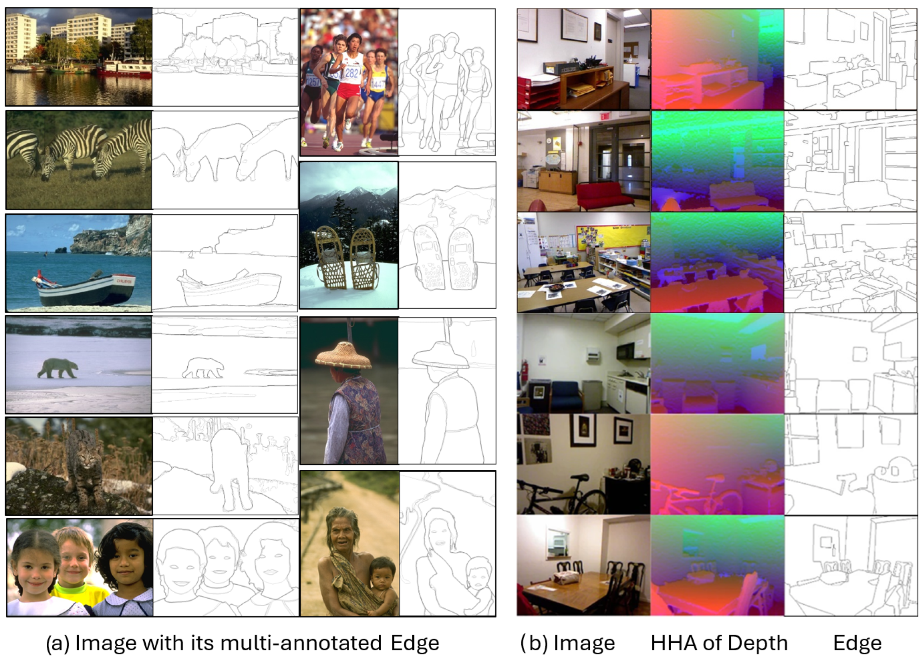
The NYU Depth Dataset V2 (NYUDv2), proposed by Silberman et al. [37] in 2012, extends edge detection to multi-modal settings. It includes 1449 RGB-D images (381 train, 414 validation, and 654 test), captured indoors at 640 × 480 resolution, with depth (D) from Kinect and hand-labeled edge maps y. Annotations cover structural boundaries (e.g., walls and furniture), available in RGB, depth (HHA format: height, horizontal disparity, and angle), or combined modalities. NYUDv2 tests the algorithms’ ability to leverage depth cues contrasting with BSDS500’s RGB-only focus (see Figure 7).

Both BSDS500 and NYUDv2 datasets are widely used benchmarks in edge detection research due to their high-quality annotations and their ability to support meaningful comparisons across a wide range of algorithms. BSDS500 is favored for its rich human-labeled edge annotations, which reflect perceptual boundaries rather than simple gradients. This makes it particularly useful for evaluating how well edge detection algorithms capture semantically meaningful structures. Its standing use in literature enables reproducible and comparable performance assessment across methods [13]. NYUDv2, on the other hand, offers indoor scenes. Its depth images help explore multi-modal edge detection. This is especially valuable for developing and evaluating methods that fuse visual and geometric cues, which are critical for robotics, AR, and indoor navigation applications [37].

Even though both datasets are relatively small in size, which can pose challenges for training large network models and hinder generalization and contribute to overfitting, it is still suitable for benchmarking and remains crucial for evaluating edge detection performance under controlled and interpretable conditions. For model development, there is a growing need to complement them with larger, more diverse datasets to train and validate models in real-world scenarios.

5.2. Evaluation Metrics

Edge detection methods typically produce edge maps, which must be thresholded to generate binary edge predictions. This is a highly imbalanced task, as edge pixels constitute a small fraction of all pixels compared to non-edge ones. Therefore, traditional performance metrics such as accuracy or Intersection over Union (IoU) are not appropriate, as they fail to capture the fine-grained nature of edge prediction.

To address this, the F-score metric—balancing precision and recall between a predicted edge map $\widehat{y}$ and the ground truth y—was introduced by Martin et al. [38] as a standard evaluation criterion for edge detection. For a given threshold T, ${\widehat{y}}_T=\{(x,y)\mid \widehat{y}(x,y)>T\}$ is binarized, and precision (P) and recall (R) are

$$P={\displaystyle \frac{|{\widehat{y}}_T\cap y|}{|{\widehat{y}}_T|}},R={\displaystyle \frac{|{\widehat{y}}_T\cap y|}{\left|y\right|}},$$

(45)

where $|·|$ denotes pixel count, accounting for a small matching tolerance (e.g., 2 pixels) due to annotation variability. The F-score is

$$F={\displaystyle \frac{2PR}{P+R}}.$$

(46)

However, the performance of an edge detection model can vary significantly depending on the threshold used to binarize the soft edge map. A threshold that works well for one image might perform poorly on another. Since selecting a single optimal threshold across an entire dataset is challenging, two evaluation metrics are commonly adopted: ODS (Optimal Dataset Scale) and OIS (Optimal Image Scale).

• ODS (Optimal Dataset Scale): measures the best F-score across the entire dataset using a single fixed threshold that is applied to all images, e.g., 0.824 for EDTER on BSDS500;
• OIS (Optimal Image Scale): measures the best F-score achieved for each individual image using its own optimal threshold, and then averages these F-scores across all images in the dataset, e.g., 0.876 for EdgeNAT on BSDS500.

ODS = 1 indicates perfect edge detection performance across the dataset at a single, fixed threshold. This means the predicted edge maps align exactly with the ground truth edges for all images: every predicted edge pixel is correct (precision = 1), and every true edge pixel is detected (recall = 1). In this case, the number of predicted features is exactly what is needed—neither too many nor too few. The model extracts just the right edges, at the correct locations and scales, and does so consistently across the entire dataset without needing per-image threshold adjustment. This ideal scenario reflects not only a powerful model but also a highly effective balance in the edge extraction process.

In contrast, ODS = 0 reflects complete failure of the edge detection model. This could happen if the model predicts no edges at all (leading to zero recall), or if it predicts many edges that do not match the ground truth (leading to zero precision), or both. In terms of feature extraction, this implies that the model either extracts too few edges (missing important structures) or far too many irrelevant or noisy edges (over-segmentation). Both the under- and over-prediction of features severely reduce the F1-score. This situation highlights the importance of both correct feature quantity and quality—extracting either too few or too many edges leads to poor precision–recall balance and thus a low ODS score.

OIS typically exceeds ODS, reflecting flexibility to image-specific thresholds. Both metrics, reported extensively in Section 3 and Section 4, quantify edge quality, with higher scores indicating better alignment with human perception.

Table 4. Comparison of key edge detection datasets. BSDS500 offers diverse RGB images with consensus edge maps, while NYUDv2 provides RGB-D pairs for multi-modal evaluation.

Dataset	Images	Modality	Ground Truth
BSDS500	500 (200/100/100)	RGB	Multiple human annotations
NYUDv2	1449 (381/414/654)	RGB-D	Structural boundaries

summarizes BSDS500 and NYUDv2, underscoring their roles in benchmarking edge detection. Together with ODS and OIS, they enable a comprehensive assessment of algorithmic progress, bridging traditional and deep learning eras.

6. Comparative Analysis and Insights

This section synthesizes edge detection’s evolution, from gradient-based methods (Section 2) to deep learning paradigms (Section 3 and Section 4), balancing high-level architectural descriptions with detailed mathematical analysis to cater to both interdisciplinary readers and experts seeking rigor (Section 2, Section 3 and Section 4). It integrates the mathematical formulations of loss functions, attention mechanisms, diffusion processes, and computational complexity with performance metrics (ODS, OIS) from

Table 5. Overall comparison of edge detection methods. ODS and OIS reflect BSDS500 and NYUDv2 accuracy (S-measure for VST on DUTS). Dashes denote unreported values.

Method	ODS (BSDS500)	OIS (BSDS500)	ODS (NYUD)	OIS (NYUD)	Paradigm
Sobel	-	-	-	-	Gradient
Canny	0.611	0.676	N/A	-	Gradient
HED	0.788	0.808	0.720	0.734	CNN
RCF	0.798	0.815	0.729	0.742	CNN
BDCN	0.806	0.826	0.748	0.763	CNN/Enc-Dec
DexiNed	0.729	0.745	0.658	0.674	CNN/Enc-Dec
NHP	0.818	0.837	0.779	0.792	CNN/Enc-Dec
AMH-Net	0.798	0.829	0.744	0.759	CNN+Attention
VST	N/A (S: 0.91)	-	-	-	Transformer
EDTER	0.824	0.841	0.774	0.789	Transformer
EdgeNAT	0.860	0.876	0.789	0.803	Transformer
RankED	0.824	0.840	0.780	0.793	Transformer Backbone
SAUGE	0.847	0.868	0.794	0.803	Transformer Backbone
DiffusionEdge	0.834	0.848	0.761	0.766	Generative
GED	0.870	0.880	-	-	Generative

and

Table 6. Computational complexity vs. ODS on BSDS500.

Method	Complexity	ODS
Sobel	$O\left(hw\right)$	0.611
HED	$O\left(Lhwc\right)$	0.788
BDCN	$O\left(Lhwc\right)$	0.806
EdgeNAT	$O\left(h^2{w}^{2}d\right)$	0.860
EDTER	$O\left(h^2{w}^{2}d\right)$	0.824
SAUGE	$O\left(h^2{w}^{2}d\right)$	0.847
GED	$O\left(TLhwc\right)$	0.870

, visualized in Figure 8 and Figure 9.

Traditional methods like Sobel and Canny (ODS 0.611) use gradient convolutions:

$$G=\sqrt{{(I\ast K_x)}^2+{(I\ast K_y)}^2},$$

(47)

where $K_x,K_y$ are Sobel kernels but struggle with noise due to fixed kernels (Section 2). CNN-based methods introduced trainable architectures. HED (ODS 0.788) employs multi-scale supervision:

$$L_{\mathrm{HED}}=-\sum _{i=1}^M\sum _j\left[y_{j}log{p}_j^{\left(i\right)}+(1-y_j)log(1-p_j^{\left(i\right)})\right],$$

(48)

where $p_j^{\left(i\right)}$ is the prediction at scale i. BDCN (ODS 0.806) refines edges with bidirectional supervision:

$$L_{\mathrm{BDCN}}=\sum _{i=1}^M\left[{\ell }_{\mathrm{BCE}}(p_i^{\mathrm{fwd}},y)+{\ell }_{\mathrm{BCE}}(p_i^{\mathrm{bwd}},y)\right],$$

(49)

enhancing continuity (Section 3.2). NHP (ODS 0.818) leverages Hadamard product fusion (Equation (20)) for robustness.

Attention-driven methods, such as EDTER (ODS 0.824) and EdgeNAT (ODS 0.860), use transformer attention described in Equation (25). The EDTER attention-based feature aggregation balances local and global cues, while the EdgeNAT SCAF-MLA decoder optimizes edge localization. Transformer backbone-based methods, RankED (ODS 0.824) and SAUGE (ODS 0.847), further advance performance. The RankED ranking loss prioritizes edge significance:

$$L_{\mathrm{RankED}}=\sum _{i,j}max(0,\alpha -(s_i-s_j)·\mathrm{sign}(r_i-r_j)),$$

(50)

with $\alpha =1$. The SAUGE diversity loss (${\lambda }_{\mathrm{diversity}}\approx 0.1$) enhances multi-scale edges. Generative models like DiffusionEdge (ODS 0.834) and GED (ODS 0.870) model edge distributions via diffusion:

$$q\left(x_t\right|x_{t-1})=\mathcal{N}(x_t;\sqrt{1-{\beta }_t}{x}_{t-1},{\beta }_{t}I),$$

(51)

where ${\beta }_t$ controls noise. The GED loss (Equation (43)) with ${\lambda }_g\approx 0.1$ achieves state-of-the-art precision.

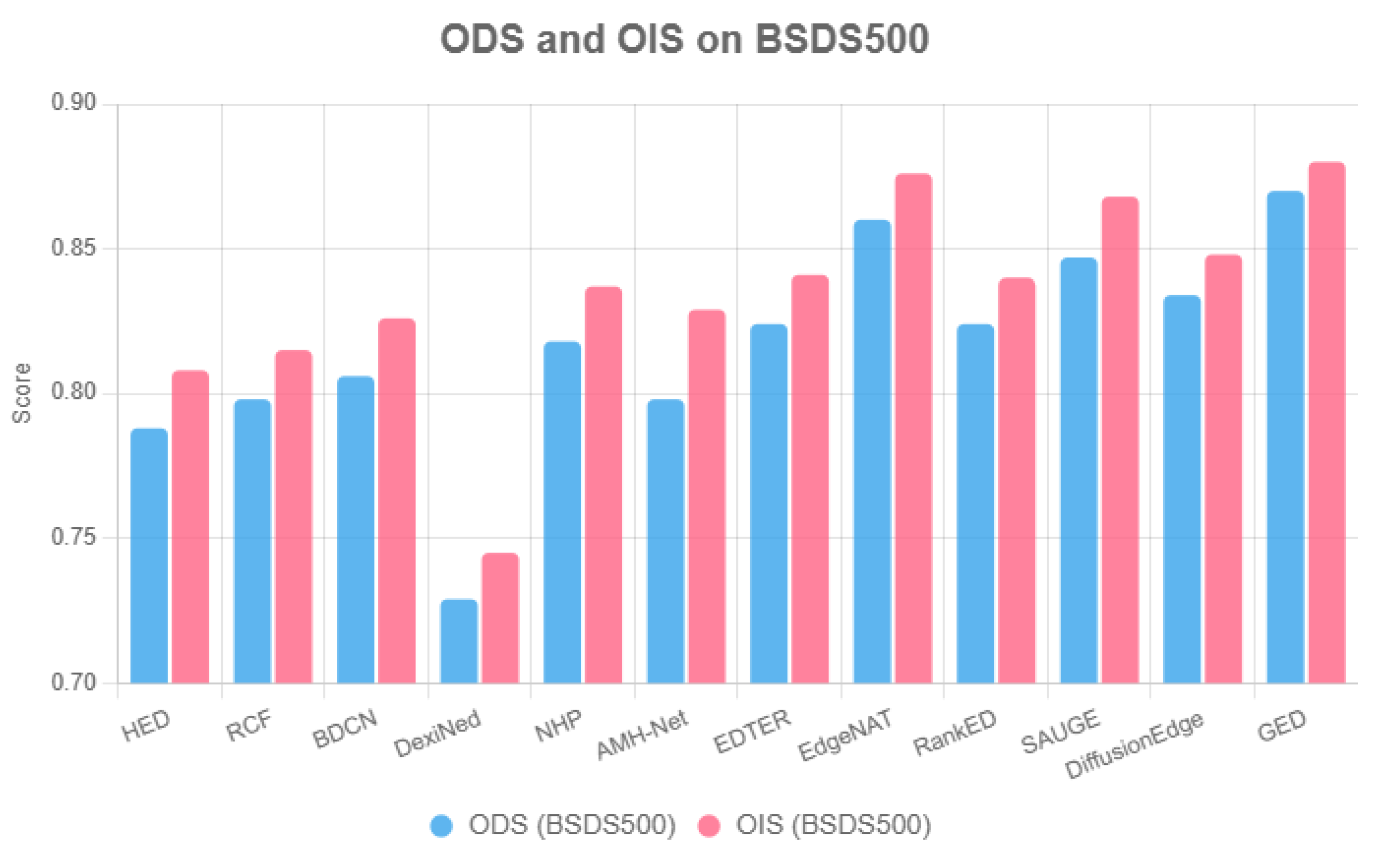
Figure 8 visualizes ODS on BSDS500, underscoring the progression from CNNs to attention-driven and generative paradigms. The GED ODS 0.870 surpasses that of EdgeNAT, at 0.860, reflecting the generative models’ ability to capture multi-scale edges as detailed in Section 4.4. However, NYUDv2 performance varies, with SAUGE (ODS 0.794) and EdgeNAT (ODS 0.789) leading, while GED lacks reported metrics, indicating generalization challenges. Traditional methods like Canny (ODS 0.611) lag significantly, limited by handcrafted kernels (Section 2).

Figure 9 compares the loss convergence of HED, BDCN, and GED, representing the CNN-based, encoder–decoder, and generative paradigms, respectively. The GED diffusion-based loss shows noticeable instability, likely due to the complexity of its optimization process and the limited size of the training dataset (BSDS500: 200 training images). In contrast, HED demonstrates stable convergence with its binary cross-entropy (BCE) loss. The dashed loss curve for EDTER is based on simulated data, as no official training loss was reported. The fluctuations observed in this attention-based method (EDTER) suggest that complex architectures may require larger training datasets to achieve stable optimization.

Mathematically, the HED local supervision (Equation (48)) limits global context, while the BDCN bidirectional loss (Equation (49)) improves continuity. The EDTER and EdgeNAT attention (Equation (25)) captures long-range dependencies, boosting ODS. The RankED ranking loss (Equation (50)) prioritizes edges, but transformer complexity poses efficiency challenges. The GED diffusion (Equation (51)) excels in edge modeling but requires stabilization, highlighting gaps in optimization and multi-modal robustness (Section 7).

Computational complexity further explains performance-efficiency trade-offs. Sobel and Canny have linear complexity, $O\left(hw\right)$, for image dimensions $h\times w$, but lack adaptability. CNN-based methods like HED and BDCN scale with $O\left(Lhwc\right)$, where c is the number of channels, and L is the network depth, balancing efficiency and accuracy. Attention-driven and transformer-based methods (EdgeNAT, EDTER, RankED, and SAUGE) incur quadratic complexity, approximately $O\left(h^2{w}^{2}d\right)$, where d is the feature dimension, due to attention mechanisms (Equation (25)). For a typical 512 × 512 image, the dimensions are $d\approx 768$∼1280, making transformers computationally heavy. Generative models like GED and DiffusionEdge require iterative sampling, with complexity $O\left(TLhwc\right)$, where T is the number of diffusion steps (e.g., $T=1000$). This high cost limits real-time applications, underscoring the need for sparse attention or efficient diffusion strategies (Section 7).

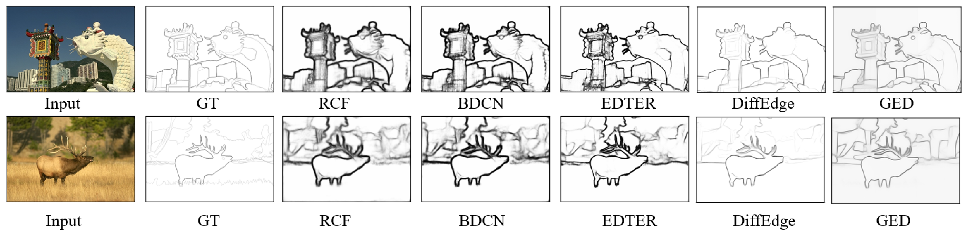
Figure 10 shows qualitative comparison of samples in the BSDS500 testset from representative methods. They are RCF, BDCN, EDTER, DiffusionEdge and GED, representing different architectural paradigms (CNN based, encoder–decoder, attention based, and generative, respectively). The examples illustrate differences in edge localization, completeness, and thickness. While CNN-based RCF produces fine-grained edges, the transformer–attention approach EDTER captures global structure but may introduce noise. Generative diffusion-based GED shows strong boundary coherence, highlighting the strengths and trade-offs across paradigms.

7. Challenges

Edge detection has evolved from gradient-based methods (Section 2) to generative paradigms (Section 4.4), achieving high precision (e.g., GED: ODS 0.870, EdgeNAT: ODS 0.860) on BSDS500 [13]. However, challenges in efficiency, generalization, and robustness limit real-world deployment. Attention-based models like EdgeNAT and SAUGE (ODS 0.847) excel in accuracy but demand high computational resources, unlike lightweight CNNs such as HED (Section 3). Generalization remains elusive, with VST’s S-measure 0.91 on DUTS [30] contrasting its BSDS500 limitations, and NYUDv2 results varying (e.g., SAUGE: ODS 0.794 vs. DiffusionEdge: 0.761). Robustness to diverse inputs, particularly in multi-modal settings like NYUDv2’s RGB-D, is underutilized beyond EdgeNAT’s HHA integration. Furthermore, Transformer-based methods (EdgeNAT, EDTER, and SAUGE) have high complexity ($O\left(n^{2}d\right)$), limiting real-time use (Table 6). Generative models (GED) require $O\left(Thw\right)$ due to iterative sampling. Future directions include sparse attention ($O(nlognd)$) and optimized diffusion schedules to reduce costs while maintaining ODS (Section 6).

8. Conclusions

This survey traces the evolution of edge detection from Sobel’s gradient-based filters to the GED generative framework, highlighting a field shaped by both mathematical and architectural innovation. Early CNN-based models such as HED (ODS 0.788) and BDCN (ODS 0.806) established the encoder–decoder paradigm (Section 3.2), which was later surpassed by attention-based approaches like EdgeNAT (ODS 0.860) and generative models such as GED (ODS 0.870) on the BSDS500 benchmark [13]. The mathematical foundations underpinning these advances—convolutions, multi-scale loss functions (Equation (48)), attention mechanisms (Equation (25)), and diffusion processes (Equation (51))—are analyzed in Section 6.

Despite significant progress, challenges remain in generalization and robustness. Transformer-based methods such as EDTER and EdgeNAT achieve strong performance (ODS 0.824–0.860) but incur the high computational complexity of $O\left(n^{2}d\right)$, while generative models like GED (ODS 0.870) face issues with training stability (Figure 9).

Future research should focus on designing more efficient architectures, such as sparse attention mechanisms [39,40] with $O(nlogn)$ complexity or hybrid CNN–transformer frameworks [41,42]. Enhancing generalization through domain-agnostic learning [43]—using self-supervised pretraining or leveraging GED diffusion priors [44]—could improve cross-dataset performance. To boost robustness, techniques like cross-modal attention [45,46] and graph-based fusion [47] hold promise for multi-modal edge detection. Furthermore, hybrid generative models that combine GED latent representations with EdgeNAT attention mechanisms may strike a balance between precision and efficiency, advancing the applicability of edge detection in domains such as robotics, medical imaging, and autonomous navigation.

This survey benefits researchers by providing (1) a clear overview of paradigms, aiding algorithm selection; (2) mathematical formulations for theoretical extensions; (3) quantitative comparisons for benchmarking; and (4) identified gaps like transformer complexity and generative instability, guiding future work. By consolidating these insights, the survey equips researchers to develop novel algorithms, optimize computational efficiency, and address challenges in generalization and robustness.