Deep Reinforcement Learning Method for Wireless Video Transmission Based on Large Deviations

Abstract

In scalable video transmission research, the video transmission process is commonly modeled as a Markov decision process, where deep reinforcement learning (DRL) methods are employed to optimize the wireless transmission of scalable videos. Furthermore, the adaptive DRL algorithm can address the energy shortage problem caused by the uncertainty of energy capture and accumulated storage, thereby reducing video interruptions and enhancing user experience. To further optimize resources in wireless energy transmission and tackle the challenge of balancing exploration and exploitation in the DRL algorithm, this paper develops an adaptive DRL algorithm that extends classical DRL frameworks by integrating dropout techniques during both the training and prediction processes. Moreover, to address the issue of continuous negative rewards, which are often attributed to incomplete training in the wireless video transmission DRL algorithm, this paper introduces the Cramér large deviation principle for specific discrimination. It identifies the optimal negative reward frequency boundary and minimizes the probability of misjudgment regarding continuous negative rewards. Finally, experimental validation is performed using the 2048-game environment that simulates wireless scalable video transmission conditions. The results demonstrate that the adaptive DRL algorithm described in this paper achieves superior convergence speed and higher cumulative rewards compared to the classical DRL approaches.

1. Introduction

The application of energy harvesting technology to power wireless transmission offers a partial solution to the energy consumption challenges in wireless video delivery systems. Energy capture technology must first model the energy capture process. Current energy harvesting models in the literature include the Bernoulli model [1,2], the dew bucket model [3] and the finite-state Markov model [4,5]. Significant contributions to this field include the work of Shenoy and Murthy (2010), who proposed throughput-optimal, delay-optimal, and delay-constrained throughput-optimal policies based on current channel-state information [6]. Subsequent research between 2014 and 2016 by Wang [7], Zarate [8], and Dang [9] maximized the utility of the system through power scheduling based on the state of energy stored in the battery. In 2015, Ku modeled the energy transmission process as a Markov decision process to minimize the time-averaged error rate in the transmission process [10]. In the same year, Chan proposed an adaptive method after modeling the energy harvesting process as a Markov decision process to balance energy storage and exploitation, thus reducing the delay and packet loss rate in energy capture [11]. To characterize the dynamics with random channel packet losses, ref. [12] introduces the state estimator using a stochastic variable in 2023. Most of the above studies on energy capture networks focus on general data transmission by adjusting power distribution and sensing data arrival to maximize system throughput or energy efficiency, but they often lack analysis of the characteristics of the data services themselves. As a result, improvements in energy exploitation rates and user experience may be insufficient. Furthermore, the inherent unpredictability and complexity of wireless network states can lead to issues such as discontinuity in energy harvesting, channel-state uncertainty, and accumulated storage during video transmission. This can result in transmission interruptions caused by insufficient energy. These technical limitations ultimately degrade the quality of user experience in video streaming applications. Machine learning algorithms, such as reinforcement learning, can autonomously and efficiently allocate network resources, making energy transmission more intelligent and effective, thus enhancing user experience. Common reinforcement learning methods include Q-learning, the actor–critic algorithm (A3C), etc. [13]. Q-learning uses Q-values to measure the quality of actions for a given state and adopts an $ϵ$-greedy policy to explore the environment, with the parameter $ϵ$ playing a crucial role [14]. To address the limitations of traditional Q-learning in large-scale problems, a deep Q-learning algorithm has been developed [15,16]. The deep Q-learning network (DQN) introduced by Mnih et al. [17] is suitable for situations with numerous states. Compared to traditional reinforcement learning algorithms [18], it incorporates deep learning techniques, compresses states, extracts features, and outputs Q-values. Using a DQN to learn and approximate Q-values enables more stable and reliable learning of the environment [19]. Subsequently, various deep reinforcement learning (DRL) algorithms have emerged. DRL is particularly effective in tasks such as industrial automation and novelty search [20,21]. Jung et al. proposed an energy storage system scheduling algorithm based on DRL that incorporates a multi-agent system and Pareto front optimization [22]. In the application of the DRL method, challenges persist due to a lack of environmental awareness. These include the well-known exploration–exploitation (EE) balance problem [23] and the complex parameter–setting problem of the Q-network [24]. Determining appropriate parameters typically requires extensive experimentation, and the rationality of these parameters can only be verified after training [25]. Therefore, the parameter setting issue is frequently overlooked and requires significant effort to resolve.

The EE problem has garnered widespread attention in the application of DRL and other model-free reinforcement learning methods [26]. Furthermore, in non-static environments, it is essential to rebalance EE promptly to adapt to environmental changes [27]. Identifying the reasons why an agent consistently receives negative rewards from the environment over a period of time is another overlooked challenge. In fact, these continued negative rewards are primarily caused by the unreasonable settings of the Q-network layers and nodes in deep Q-learning, or by training that halts before completion. Previous studies typically attribute continued negative rewards to incomplete training, while the impact of the unreasonable layer and node settings in deep networks has been neglected, leading to misjudgments and excessive time spent waiting for network model convergence. Zhu et al. first proposed using the large deviation principle (LDP) [28,29] to determine the optimal boundary [27]. However, their analysis did not rigorously derive the optimal boundary under different cases with the LDP.

Based on energy capture technology and the LDP from limit theory, this paper focuses on the realization of adaptive wireless video transmission and the prediction of the rationality of deep network parameter designs. It investigates the resource optimization problem of scalable wireless video transmission driven by energy capture technology to enhance network communication efficiency. First, according to [27], the network requirements for video data and the amount of captured energy are important. This paper introduces an adaptive DRL algorithm capable of realizing adaptive wireless transmission of scalable video as environmental conditions change. Specifically, dropout technology is introduced and applied in both the training process and the prediction process, allowing the same input to propagate forward multiple times to obtain different Q-value predictions. From these, we derive a Q-value prediction distribution and determine the optimal policies by maximizing the sampled Q-values. This approach avoids the exploration–exploitation dilemma and reduces the number of hyperparameters. Additionally, since the training in this paper yields a predictive distribution of Q-values, the new algorithm becomes more adaptive and can quickly and adaptively address the resource allocation problem in scalable wireless video transmission driven by energy capture technology. Adaptive DRL algorithms are very useful in solving practical problems [30]. Second, by introducing the large deviation principle to minimize the probability of misjudgment, a criterion is proposed to evaluate whether the Q-network is appropriately set before training concludes. This criterion can help identify why the agent consistently receives negative rewards from the environment in a certain period of time, thereby saving substantial time and resources in Q-network parameter selection. Finally, experimental validation was conducted using the 2048 game, a simple and engaging number puzzle game, and the results indicate that the adaptive DRL algorithm described in this thesis demonstrates superior adaptability in the 2048 game, achieving faster convergence and higher rewards. This suggests that the method can more rapidly adapt to environmental changes, effectively manage video clarity transitions, and enhance the user’s viewing experience in scalable wireless video transmission, thereby validating the feasibility of the proposed method for optimizing wireless frequency transmission.

The rest of this paper is organized as follows: In Section 2, after modeling the wireless video transmission process as a Markov decision process, we introduce uncertainty into traditional DRL and establish a deep Q-learning algorithm that can realize adaptive video transmission. In Section 3, the Cramér large deviation principle is used to determine the optimal boundary for the number of continuous negative rewards in the observation window, specifically distinguishing the reasons for continuous negative rewards in the training process to minimize the probability of misjudgment and improve the model’s training and operational efficiency. Section 4 simulates the scalable wireless video transmission environment using the 2048 game. Finally, concluding remarks are presented in Section 5.

2. Adaptive Wireless Video Transmission Based on Deep Q-Learning

Scalable video coding technology is the preferred method for achieving high-quality video services [31]. It designs the encoded video stream as a layered structure, which mainly includes a basic layer and several enhancement layers. The basic layer ensures minimum video quality, while the enhancement layers provide video images of different quality levels depending on network conditions. Therefore, dynamically switching enhancement layers can effectively control the bitstream of video streaming, ultimately enabling adaptive video transmission in wireless communication systems. In this section, we apply energy capture technology to video streaming services and propose an adaptive transmission strategy for scalable videos.

To address the challenges of video transmission using reinforcement learning, we first model the video transmission process as a Markov decision process $\langle \mathcal{S},\mathcal{A},\mathcal{P},\mathcal{R},\gamma \rangle$, where $\mathcal{S}$ is the set of states $s_t$ at time $t,t=1,2,\cdots ,$$\mathcal{A}$ is the set of actions $a_t,r_t$ is the reward for the transition from $s_{t-1}$ to $s_t$, $\mathcal{P}$ is the transition probability matrix, and $\gamma$ is the discount factor for long-term rewards.

However, in practical applications, this model may frequently switch video articulation, which can negatively affect the user experience. To reduce fluctuations in video quality, we incorporate the number of invalid action movements N as a penalty to adjust the value of reward function $\mathcal{R}$. When the enhancement layer switches frequently, a corresponding negative reward value n is assigned to guide the learning behavior.

Let the value function $Q_{\pi }(s,a)$ represent the action-value function of the agent based on the policy $\pi$, which represents the expected value of the return obtained by adopting the strategy $\pi$ and performing action a starting from state s. Its specific expression is given by

$$Q_{\pi }(s,a)=E[R_{t+1}+\gamma R_{t+2}+\cdots |S_t=s,A_t=a].$$

According to the Bellman equation, we can derive the following Bellman expectation equation:

$$Q_{\pi }(s,a)=E[R_{t+1}+\gamma Q_{\pi }(S_{t+1},A_{t+1})|S_t=s,A_t=a].$$

In reinforcement learning, there is always an optimal strategy ${\pi }^{*}$ that is superior to or at least equal to other strategies [32]. This optimal strategy is not necessarily unique, but the state-value function under the optimal strategy must be equal to the optimal state-value function, and the action-value function must be equal to the optimal action-value function. Therefore, by calculating $Q(s_t,a_t)$ for all actions $a_t$ in state $s_t$, we can ultimately choose the optimal action $a=arg\underset{a\in \mathcal{A}}{max}{Q}^{*}(s,a)$ with probability $ϵ$, or randomly select an action with probability $1-ϵ$, thereby obtaining the optimal strategy. The specific method is as follows:

$$\begin{array}{c}\hfill {\pi }^{*}\left(a\right|s)=\left\{\begin{array}{cc}1,\hfill & a=arg\underset{a\in \mathcal{A}}{max}{Q}^{*}(s,a),\hfill \\ 0,\hfill & otherwise.\hfill \end{array}\right.\end{array}$$

Specially, $Q^{*}(s,a)=\underset{\pi }{max}{Q}_{\pi }(s,a)$ is the optimal action-value function.

Next, we establish a deep Q-learning algorithm capable of realizing adaptive video transmission. In the classical deep Q-learning algorithm, the hyperparameter $\epsilon$ plays a crucial role in regulating the balance between exploration and exploitation. To maximize cumulative rewards, an appropriate compromise between exploration and exploitation must be selected. One simple and often successful method for achieving this balance is the $\epsilon$-greedy strategy [33]. This strategy does not require memory of exploration-specific data, making it especially suitable for complex models with particularly large or continuous state spaces. However, the $\epsilon$-greedy algorithm has an obvious disadvantage in practice: it is not immediately clear how to set a specific $\epsilon$ value for a given learning task to yield good learning results. Manually setting this compromise value can be a time-consuming task in practice as it depends on the complexity of the target model. Moreover, when the environment changes, the classical deep Q-learning algorithm simply struggles to rebalance exploration and exploitation promptly, causing previously trained strategies to fail to update accordingly. Therefore, this chapter proposes an adaptive deep Q-learning method that automatically achieves a balance between exploration and exploitation and timely updates the policy. This method reduces the number of hyperparameters that must be adjusted, facilitating further optimization of the model.

In the adaptive deep Q-learning method, according to [27], we introduce dropout technology, applying it to both the training process and the prediction process of Q-networks. Consequently, the output value of the Q-network becomes a random variable following a Gaussian distribution [34]. This characteristic, where the same input value can yield different results, means that each dropout results in the training of a “completely new” network. Ultimately, this ensemble of networks enhances and constrains each other, leading to improved final results. Specifically, this thesis passes the same input value forward $N_f$ times, calculating the mean and variance of $N_f$ predictions to represent the predicted value of the Q-value and the uncertainty of the prediction, respectively. The predicted mean and variance are then taken as the mean and variance of the Gaussian distribution, resulting in the prediction distribution of the Q-network. During action selection, random sampling is performed within this prediction distribution, and the action with the largest Q-value is selected based on the sampled Q-network. In this model, greater uncertainty leads to higher prediction variance, resulting in more randomness from the Q-network obtained through sampling. In such cases, action selection serves an exploratory role. Conversely, lower uncertainty corresponds to smaller prediction variance, leading to a more concentrated Q-network and values closer to the predicted mean, thereby causing the selected action to be closer to the optimal action. In this case, action selection serves an exploitation role. With continuous training, the sampled values will approximate the average value of the Gaussian distribution and gradually converge, ultimately yielding the global optimal strategy. The above adaptive deep Q-learning algorithm is illustrated below in Algorithm 1.    

Algorithm 1: Adaptive deep Q-learning algorithm

1: Initialize the experience playback experience pool D;  2: Initialize the neural network with random weights, and obtain the initial Q function;  3: Initialize the number of forward passes $N_f$;  4: for$episode=1toM$do  5:     Initialize state $s_1$;  6:     for $t=1toN$ do  7:         for $i=1to{N}_f$ do  8:             Use the neural network and dropout technology to predict the input state;  9:             Store Q-function in $Q_{list}$;  10:       end for  11:       $Q_{mean}=\mathrm{E}\left[Q_{list}\right],Q_{var}=\mathrm{Var}\left(Q_{list}\right);$  12:       Sample from distribution $N\left(Q_{mean},Q_{var}\right)$;  13:       Get $Q^{*}$;  14:       Select the action $a_t$ that maximizes $Q^{*}$;  15:       Perform the selected action $a_t$;  16:       Get return $r_t$ and next state $s_{t+1}$;  17:       $D\leftarrow D+<s_t,a_t,r_t,s_{t+1}>$;  18:       Sample randomly from D;  19:       Get m samples $<s_j,a_j,r_j,s_{j+1}>$;  20:       Set the sample label value $${\pi }^{*}\left(a\right|s)=\left\{\begin{array}{cc}{r}_j,\hfill & s_{j+1}isterminal,\\ r_j+\gamma \underset{a_{j+1}}{max}Q\left(s_{j+1},a_{j+1};\theta \right),\hfill & otherwise.\hfill \end{array}\right.$$  21:       Update network parameters with the gradient descent method;  22:   end for  23: end for

3. Misjudgment Probability Control Based on Large Deviation Principle

In the process of deep Q-learning training, the agent sometimes receives a continuous negative reward, resulting in a negative cumulative reward over a certain period. This outcome contradicts the original goal of achieving higher reward values in reinforcement learning. There are generally two reasons for this phenomenon. One reason is that the layer and node configurations of the Q-network in deep Q-learning are incorrect, leading to excessive deviation in the Q-value estimation. The other reason is that the training process is incomplete and requires more time to complete the training. In the second case, we often simply wait for the Q-network to converge when facing a persistent negative reward problem. However, if this persistent negative reward issue arises from the first case, it may be difficult or even impossible for the Q-network to converge. To avoid such situations, this chapter proposes a reasonable criterion for setting the Q-network based on the principle of a large deviation, which is aimed at reducing the misjudgment probability of rare events.

In the specific wireless video transmission example, let n denote the length of the observation window. Suppose event ${\mathfrak{A}}_{ur}$ represents a negative reward caused by an unreasonable setting of the Q-network’s layers and nodes, with its probability denoted as $p_{ur}=P\left({\mathfrak{A}}_{ur}\right)$. We define a sequence of random variables ${\xi }_t,t=1,2,\cdots$ to represent the positive and negative reward situations within the observation window. Specifically, $({\xi }_t=1)$ indicates that the reward at the $t$-th observation point in the observation window is negative, while $({\xi }_t=0)$ indicates that the reward of the $t$-th observation point in the observation window is non-negative. In this thesis, we assume that ${\xi }_t,t=1,2,\cdots$ forms an independent and identically distributed sequence of random variables. Let event $B_2$ indicate that the training process has completed. Then $\left({\xi }_t\right|B_2=1)$ indicates that event ${\mathfrak{A}}_{ur}$ occurs. Thus, under the condition that event $B_2$ occurs, ${\xi }_t$ follows a Bernoulli distribution, with the probability mass function defined as follows in

Table 1. Distribution of ${\xi }_t|B_2$.

${\mathit{\xi }}_{\mathit{t}}|{\mathit{B}}_2$	0	1
P	$1-p_{ur}$	$p_{ur}$

.

Assume event $\mathfrak{A}$ indicates that the training is incomplete and negative rewards appear, and event ${\mathfrak{A}}_{uf}$ indicates that training is incomplete and results in a negative reward; we have $\mathfrak{A}={\mathfrak{A}}_{ur}\cup {\mathfrak{A}}_{uf}$; that is, an unreasonable network setting or incomplete training may lead to a negative reward. The probabilities $p^{\prime }=P\left(\mathfrak{A}\right)$ and $p_{uf}=P\left({\mathfrak{A}}_{uf}\right)$ represent the occurrence of events $\mathfrak{A}$ and ${\mathfrak{A}}_{uf}$, respectively. Assuming that the event of an incomplete training process and the event of an improper network setting are independent. We can obtain the equality as follows:

$$\begin{array}{ccc}\hfill P\left(\mathfrak{A}\right)& =& P({\mathfrak{A}}_{ur}\cup {\mathfrak{A}}_{uf})\hfill \\ & =& P\left({\mathfrak{A}}_{ur}\right)+P\left({\mathfrak{A}}_{uf}\right)-P({\mathfrak{A}}_{ur}\cap {\mathfrak{A}}_{uf})\hfill \\ & =& P\left({\mathfrak{A}}_{ur}\right)+P\left({\mathfrak{A}}_{uf}\right)-P\left({\mathfrak{A}}_{ur}\right)·P\left({\mathfrak{A}}_{uf}\right).\hfill \end{array}$$

$$i.e.,p^{\prime }=p_{ur}+p_{uf}-p_{ur}·p_{uf}.$$

Let event $B_1$ indicate that the training is incomplete; then $\left({\xi }_t\right|B_1=1)$ indicates that event $\mathfrak{A}$ occurs. Therefore, under the condition that event $B_1$ occurs, ${\xi }_t$ follows a Bernoulli distribution with the probability mass function defined as follows in

Table 2. Distribution of ${\xi }_t|B_1$.

${\mathit{\xi }}_{\mathit{t}}|{\mathit{B}}_1$	0	1
P	$1-p^{\prime }$	$p^{\prime }$

.

Since n denotes the length of the observation window in wireless video transmission, the number of negative rewards in the observation window is denoted as $m(m=0,1,2,\cdots ,n)$. Obviously, the occurrence of a continuous negative reward in the observation window under the condition of event $B_1$ corresponds to the occurrence of event $\mathfrak{A}$; that is, the occurrence of a continuous negative reward is due to unreasonable network settings or incomplete training. Combined with the distribution of the random variable sequence $\left\{{\xi }_t\right|B_1\}$, we can obtain the probability distribution of the event such that the negative reward appears m times in the observation window when event $B_1$ occur; the detail is as follows:

$$P\left(m\right|B_1)\triangleq P\left(\sum _{t=1}^n{\xi }_t=m|B_1\right)=\left(\begin{array}{c}n\\ m\end{array}\right){\left(p^{\prime }\right)}^m{(1-p^{\prime })}^{n-m}.$$

The occurrence of a continuous negative reward in the observation window under the condition of event $B_2$ corresponds to the occurrence of ${\mathfrak{A}}_{ur}$; that is, the occurrence of a continuous negative reward is caused by unreasonable network settings. Combined with the distribution of the random variable sequence $\left\{{\xi }_t\right|B_2\}$, we can obtain the probability distribution of the event such that the negative reward appears m times in the observation window when event $B_2$ occurs; the detail is as follows:

$$P\left(m\right|B_2)\triangleq P\left(\sum _{t=1}^n{\xi }_t=m|B_2\right)=\left(\begin{array}{c}n\\ m\end{array}\right){\left(p_{ur}\right)}^m{(1-p_{ur})}^{n-m}.$$

According to Bayes’ formula [35], we can express the conditional probabilities of events $B_1$ and $B_2$ when the negative reward occurs m times in the observation window, where

$$\begin{array}{c}\hfill P\left(B_1\right|m)\triangleq P\left(B_1|\sum _{t=1}^n{\xi }_t=m\right)={\displaystyle \frac{P\left(m\right|B_1)·P\left(B_1\right)}{P\left({\displaystyle \sum _{t=1}^n}{\xi }_t=m\right)}},\end{array}$$

(1)

$$\begin{array}{c}\hfill P\left(B_2\right|m)\triangleq P\left(B_2|\sum _{t=1}^n{\xi }_t=m\right)={\displaystyle \frac{P\left(m\right|B_2)·P\left(B_2\right)}{P\left({\displaystyle \sum _{t=1}^n}{\xi }_t=m\right)}}.\end{array}$$

(2)

Based on the principle of minimum deviation estimation [27,36], we define a statistical criterion to distinguish whether the continuous negative rewards are due to incomplete training or an improperly configured Q-network as follows:

$$\begin{array}{c}\hfill P\left(m\right|B_2)>{\displaystyle \frac{P\left(m\right|B_1)}{\alpha }}.\end{array}$$

(3)

where $\alpha =P\left(B_2\right)/P\left(B_1\right)$.

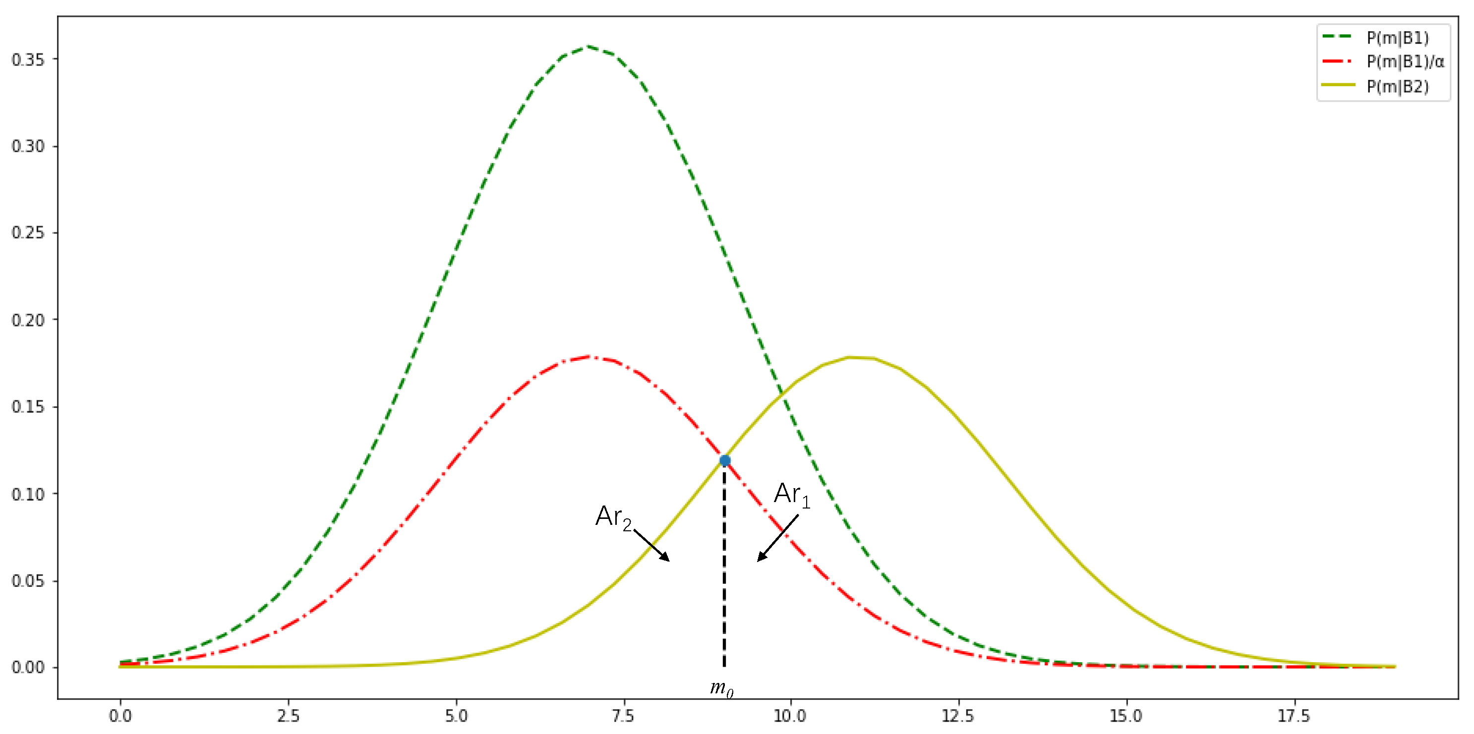
To intuitively understand this statistical criterion, we can plot the distribution function of the conditional probability, as shown in Figure 1, where $m_0$ denotes the upper bound on the number of negative reward occurrences.

As seen in the figure above, as long as the value of the frequency of the negative reward occurs in the observation window ${\displaystyle \sum _{t=1}^n}{\xi }_t=m\ge m_0$, inequality $\left(\right)$ holds. At this point, we can conclude that the training process is complete, meaning that $m_0$ can be used as a boundary for the frequency of continuous negative rewards. Based on this, we can define the criterion for determining the cause of continuous negative rewards using the adaptive DRL method as follows: If $m\ge m_0$, the negative reward is considered to result from unreasonable network settings. If $m<m_0$, the negative reward is attributed to an incomplete training process.

When the training process is incomplete, event $B_1$ occurs; if $m\ge m_0$, we conclude that the negative reward occurs due to unreasonable network settings. Conversely, when the training process is completed, event $B_2$ occurs; if $m<m_0$, we judge that the negative reward is due to the training process not being completed. To reduce the probability of misjudgment, calculate the probability of these two misjudgments separately. Let $A{r}_1=P({\displaystyle \sum _{t=1}^n}{\xi }_t\ge m_0|B_1)$ represent the probability that a negative reward in the observation window occurs more than $m_0$ when training is incomplete; let $A{r}_2=P({\displaystyle \sum _{t=1}^n}{\xi }_t<m_0|B_2)$ represent the probability that a negative reward in the observation window occurs less than $m_0$ under the condition that the training process has been completed. Define $P_{mis}$ as the probability that the final judgment result is wrong; we have

$$\begin{array}{ccc}\hfill P_{mis}& =& P\left(\sum _{t=1}^n{\xi }_t\ge m_0,B_1\right)+P\left(\sum _{t=1}^n{\xi }_t<m_0,B_2\right)\hfill \\ & =& P\left(B_1\right)P\left(\sum _{t=1}^n{\xi }_t\ge m_0|B_1\right)+P\left(B_2\right)P\left(\sum _{t=1}^n{\xi }_t<m_0|B_2\right)\hfill \\ & =& P\left(B_1\right)A{r}_1+P\left(B_2\right)A{r}_2.\hfill \end{array}$$

The following Theorem 1 shows how to determine the boundary $m_0$ to minimize the probability of an error in the final judgment $P_{mis}$ for the length of the observation window n.

Theorem 1.

Given the length of the observation window n, the optimal boundary $m_0$, which makes the final judgment result reach the minimum error probability $P_{mis}=P\left(B_1\right)A{r}_1+P\left(B_2\right)A{r}_2$, can be determined by

$$\begin{array}{c}\hfill \underset{m_0}{inf}P\left(B_1\right)A{r}_1+P\left(B_2\right)A{r}_2,\end{array}$$

(4)

with the conditions on $m_0$ defined as follows:

$$\begin{array}{c}\hfill P\left(B_1\right)A{r}_1+P\left(B_2\right)A{r}_2\sim \left\{\begin{array}{cc}P\left(B_1\right)\left(1-exp\left(-n{I}_{\xi |B_1}\left({\displaystyle \frac{m_0}{n}}\right)\right)\right)+P\left(B_2\right)exp\left(-n{I}_{\xi |B_2}\left({\displaystyle \frac{m_0}{n}}\right)\right),\hfill & m_0<n{p}_{ur};\hfill \\ P\left(B_1\right)\left(1-exp\left(-n{I}_{\xi |B_1}\left({\displaystyle \frac{m_0}{n}}\right)\right)\right)+P\left(B_2\right)\left(1-exp\left(-n{I}_{\xi |B_2}\left({\displaystyle \frac{m_0}{n}}\right)\right)\right),\hfill & n{p}_{ur}<m_0<n{p}^{\prime };\hfill \\ P\left(B_1\right)exp\left(-n{I}_{\xi |B_1}\left({\displaystyle \frac{m_0}{n}}\right)\right)+P\left(B_2\right)\left(1-exp\left(-n{I}_{\xi |B_2}\left({\displaystyle \frac{m_0}{n}}\right)\right)\right),\hfill & m_0>n{p}^{\prime },\hfill \end{array}\right.\end{array}$$

where $I_{\xi |B_1}\left({\displaystyle \frac{m_0}{n}}\right)={\displaystyle \frac{m_0}{n}}log\left({\displaystyle \frac{m_0}{n{p}^{\prime }}}\right)+(1-{\displaystyle \frac{m_0}{n}})log\left({\displaystyle \frac{n-m_0}{n(1-p^{\prime })}}\right)$ and $I_{\xi |B_2}\left({\displaystyle \frac{m_0}{n}}\right)={\displaystyle \frac{m_0}{n}}log\left({\displaystyle \frac{m_0}{n{p}_{ur}}}\right)+(1-{\displaystyle \frac{m_0}{n}})log\left({\displaystyle \frac{n-m_0}{n(1-p_{ur})}}\right)$ are the rate functions of random variable sequences $\left\{{\xi }_t\right|B_1\}$ and $\left\{{\xi }_t\right|B_2\}$, respectively.

Proof. 

During training, it is a small-probability event that the frequency of negative rewards within the observation window reaches or exceeds $m_0$ before training is complete. Similarly, the frequency of negative rewards within the observation window after training completion can also be considered as a small-probability event. We use the random variable sequences $\left\{{\xi }_t\right|B_1\}$ and $\left\{{\xi }_t\right|B_2\}$ to describe the occurrence probabilities of these two events, yielding the following two formulas:

$$A{r}_1=P\left(\sum _{t=1}^n{\xi }_t\ge m_0|B_1\right)=P\left(\omega :{\displaystyle \frac{{\xi }_1\left(\omega \right)+\cdots +{\xi }_n\left(\omega \right)}{n}}\ge {\displaystyle \frac{m_0}{n}}|B_1\right),$$

$$A{r}_2=P\left(\sum _{t=1}^n{\xi }_t<m_0|B_2\right)=P\left(\omega :{\displaystyle \frac{{\xi }_1\left(\omega \right)+\cdots +{\xi }_n\left(\omega \right)}{n}}<{\displaystyle \frac{m_0}{n}}|B_2\right).$$

To analyze these small-probability events, we apply Cramér theorem [24]. Given that the random variable sequences $\left\{{\xi }_t\right|B_1\}$ and $\left\{{\xi }_t\right|B_2\}$ follow Bernoulli distributions, their moment-generating functions are defined as follows:

$$E\left[exp\left(\theta {\xi }_t\right|B_1)\right]=1-p^{\prime }+p^{\prime }{e}^{\theta },$$

$$E\left[exp\left(\theta {\xi }_t\right|B_2)\right]=1-p_{ur}+p_{ur}{e}^{\theta }.$$

Clearly, for any $\theta >0$, we have $E\left[exp\left(\theta {\xi }_t\right|B_1)\right]<\infty$ and $E\left[exp\left(\theta {\xi }_t\right|B_2)\right]<\infty$. This satisfies the conditions of Cramér’s theorem [28,37], indicating that the random variable sequences $\left\{{\xi }_t\right|B_1\}$ and $\left\{{\xi }_t\right|B_2\}$ satisfy a large deviation principle with convex rate functions $I_{\xi |B_1}\left(x\right)$ and $I_{\xi |B_2}\left(x\right)$. For any $\epsilon >0$, we have

$$\begin{array}{c}\hfill P\left(\left(|{\displaystyle \frac{{\xi }_1+\cdots +{\xi }_n}{n}}-E\xi |\ge \epsilon \right)|B_i\right)\sim exp\left(-n{I}_{\xi |B_i}\left(x\right)\right),i=1,2.\end{array}$$

i.e.,

$$\begin{array}{c}\hfill P\left(\left({\displaystyle \frac{{\xi }_1+\cdots +{\xi }_n}{n}}\ge \epsilon +E\xi \right)|B_i\right)\sim exp\left(-n{I}_{\xi |B_i}\left(x\right)+o\left({\displaystyle \frac{1}{n}}\right)\right),i=1,2.\end{array}$$

or

$$\begin{array}{c}\hfill P\left(\left({\displaystyle \frac{{\xi }_1+\cdots +{\xi }_n}{n}}\le -\epsilon +E\xi \right)|B_i\right)\sim exp\left(-n{I}_{\xi |B_i}\left(x\right)+o\left({\displaystyle \frac{1}{n}}\right)\right),i=1,2.\end{array}$$

where $x=\epsilon +E\xi$ or $x=-\epsilon +E\xi$.

According to Cramér theorem and the Legendre transform [37,38], we have the following convex rate functions

$$\begin{array}{c}\hfill I_{\xi |B_1}\left(x\right)=\underset{\theta \in R}{sup}\{x\theta -logE\left[exp\left(\theta {\xi }_t\right|B_1)\right]\},\end{array}$$

(5)

$$\begin{array}{c}\hfill I_{\xi |B_2}\left(x\right)=\underset{\theta \in R}{sup}\{x\theta -logE\left[exp\left(\theta {\xi }_t\right|B_1)\right]\}.\end{array}$$

(6)

For Formula $\left(5\right)$, take

$$\begin{array}{ccc}\hfill f\left(\theta \right)& =& x\theta -logE\left[exp\left(\theta {\xi }_t\right|B_1)\right]\hfill \\ & =& x\theta -log(1-p^{\prime }+p^{\prime }{e}^{\theta }).\hfill \end{array}$$

Derive $f\left(\theta \right)$ with respect to $\theta$; we see that $f\left(\theta \right)$ is monotonically decreasing, and $f\left(\theta \right)$ obtains the maximum value when

$${\theta }^{*}=log\left({\displaystyle \frac{x(1-p^{\prime })}{(1-x)p^{\prime }}}\right).$$

Now

$$\begin{array}{ccc}\hfill I_{\xi |B_1}\left(x\right)& =& x\theta -log(1-p^{\prime }+p^{\prime }exp\left({\theta }^{*}\right))\hfill \\ & =& xlog\left({\displaystyle \frac{x}{p^{\prime }}}\right)+(1-x)log\left({\displaystyle \frac{1-x}{1-p^{\prime }}}\right).\hfill \end{array}$$

The same is true for Formula $\left(6\right)$

$$\begin{array}{ccc}\hfill I_{\xi |B_2}\left(x\right)& =& x\theta -log(1-p_{ur}+p_{ur}exp\left({\theta }^{**}\right))\hfill \\ & =& xlog\left({\displaystyle \frac{x}{p_{ur}}}\right)+(1-x)log\left({\displaystyle \frac{1-x}{1-p_{ur}}}\right).\hfill \end{array}$$

Specially,

$${\theta }^{**}=log\left({\displaystyle \frac{x(1-p_{ur})}{(1-x)p_{ur}}}\right).$$

To sum up,

(1)

When ${\displaystyle \frac{m_0}{n}}<p_{ur}$, it follows that ${\displaystyle \frac{m_0}{n}}<p_{ur}<p^{\prime }.$ In this case, the probabilities of committing Type I and Type II errors are given by

$$\begin{array}{ccc}\hfill A{r}_1& =& P\left(\omega :{\displaystyle \frac{{\xi }_1\left(\omega \right)+\cdots +{\xi }_n\left(\omega \right)}{n}}\ge {\displaystyle \frac{m_0}{n}}|B_1\right)\hfill \\ & =& 1-P\left(\omega :{\displaystyle \frac{{\xi }_1\left(\omega \right)+\cdots +{\xi }_n\left(\omega \right)}{n}}<{\displaystyle \frac{m_0}{n}}|B_1\right)\hfill \\ & \sim & 1-exp\left(-n{I}_{\xi |B_1}\left({\displaystyle \frac{m_0}{n}}\right)\right);\hfill \end{array}$$

(7)

$$\begin{array}{ccc}\hfill A{r}_2& =& P\left(\omega :{\displaystyle \frac{{\xi }_1\left(\omega \right)+\cdots +{\xi }_n\left(\omega \right)}{n}}<{\displaystyle \frac{m_0}{n}}|B_2\right)\hfill \\ & \sim & exp\left(-n{I}_{\xi |B_2}\left({\displaystyle \frac{m_0}{n}}\right)\right).\hfill \end{array}$$

(2)

When $p_{ur}<{\displaystyle \frac{m_0}{n}}<p^{\prime }$, the probability of committing a Type I error equals to Equation (7) due to the condition $p^{\prime }>{\displaystyle \frac{m_0}{n}}$. Similarly, under $p_{ur}<{\displaystyle \frac{m_0}{n}}$, the probability of committing a Type II error is given by

$$\begin{array}{ccc}\hfill A{r}_2& =& P\left(\omega :{\displaystyle \frac{{\xi }_1\left(\omega \right)+\cdots +{\xi }_n\left(\omega \right)}{n}}<{\displaystyle \frac{m_0}{n}}|B_2\right)\hfill \\ & =& 1-P\left(\omega :{\displaystyle \frac{{\xi }_1\left(\omega \right)+\cdots +{\xi }_n\left(\omega \right)}{n}}\ge {\displaystyle \frac{m_0}{n}}|B_2\right)\hfill \\ & \sim & 1-exp\left(-n{I}_{\xi |B_2}\left({\displaystyle \frac{m_0}{n}}\right)\right).\hfill \end{array}$$

(8)

(3)

When ${\displaystyle \frac{m_0}{n}}>p^{\prime }$, the probability of committing a Type I error is

$$\begin{array}{ccc}\hfill A{r}_1& =& P\left(\left(\omega :{\displaystyle \frac{{\xi }_1\left(\omega \right)+\dots +{\xi }_n\left(\omega \right)}{n}}\ge {\displaystyle \frac{m_0}{n}}\right)|B_1\right)\hfill \\ & \sim & exp\left(-n{I}_{\xi |B_1}\left({\displaystyle \frac{m_0}{n}}\right)\right);\hfill \end{array}$$

And according to $p_{ur}<p^{\prime }<{\displaystyle \frac{m_0}{n}}$, we see that the probability of committing a Type II error is the same as in Equation $\left(8\right)$.

The optimal decision boundary $m_0$ that minimizes the overall error probability can be determined through the following calculation:

$$\begin{array}{c}\hfill P\left(B_1\right)A{r}_1+P\left(B_2\right)A{r}_2\sim \left\{\begin{array}{cc}P\left(B_1\right)\left(1-exp\left(-n{I}_{\xi |B_1}\left({\displaystyle \frac{m_0}{n}}\right)\right)\right)+P\left(B_2\right)exp\left(-n{I}_{\xi |B_2}\left({\displaystyle \frac{m_0}{n}}\right)\right),\hfill & m_0<n{p}_{ur};\hfill \\ P\left(B_1\right)\left(1-exp\left(-n{I}_{\xi |B_1}\left({\displaystyle \frac{m_0}{n}}\right)\right)\right)+P\left(B_2\right)\left(1-exp\left(-n{I}_{\xi |B_2}\left({\displaystyle \frac{m_0}{n}}\right)\right)\right),\hfill & n{p}_{ur}<m_0<n{p}^{\prime };\hfill \\ P\left(B_1\right)exp\left(-n{I}_{\xi |B_1}\left({\displaystyle \frac{m_0}{n}}\right)\right)+P\left(B_2\right)\left(1-exp\left(-n{I}_{\xi |B_2}\left({\displaystyle \frac{m_0}{n}}\right)\right)\right),\hfill & m_0>n{p}^{\prime },\hfill \end{array}\right.\end{array}$$

where $I_{\xi |B_1}\left(x\right)$ and $I_{\xi |B_2}\left(x\right)$ are the rate functions of random variable sequences (see Equations $\left(5\right)$ and $\left(6\right)$ for details).    □

The optimal boundary in [27] is not rigorously derived using the LDP. Based on the specific results of Theorem 1, we derive the Algorithm 2 illustrated below.

Algorithm 2: The discrimination algorithm for the cause of a persistent negative reward

Initialize the length of the observation window n; Initialize the number of negative rewards in the observation window m; Calculate the boundary of the frequency ($m_0$) that a continuous negative reward occurs according to Formula $\left(4\right)$; for $t=1,2\cdots$ do     Select action $a_t$ according to the algorithm in Figure 1;     Perform action $a_t$ and get reward $r_t$;     if $r_t<0$ then         $m=m+1$;     end if end for if  $m>m_0$  then      Judge that the Q-network settings are unreasonable, and reset Q-network parameters; else      Judge that the training is not complete, and retrain the Q-network; end if

After obtaining the optimal boundary $m_0$, we can judge the reason for the occurrence of continuous negative rewards by comparing the size of $m_0$ with the actual occurrence of negative rewards m in the observation window. When $m\ge m_0$, we have sufficient reason to think that the reason for the continuous negative reward is due to an unreasonable network setting; when $m<m_0$, we have sufficient reason to think that the reason for the continuous negative reward is due to the incomplete training process.

4. Simulation Experiment

The 2048 game is a popular strategy game released by Gabrielle on Github in 2014. This chapter considers using the classic 2048 game as a simulation model for the wireless video transmission process, as both of them share a similar structure based on a Markov decision process structure with a huge number of states and a limited number of actions.

4.1. Introduction of the Game Model and Game Setting

The 2048 game consists of a $4\times 4$ grid, comprising a total of 16 rectangular areas. The specific structure of the game is illustrated in Figure 2. At the beginning of the game, a number square will be generated in any 2 of the 16 positions, with the value being either two or four. Players can choose one direction to slide the squares each turn; all number squares will move toward the selected direction. When squares with the same number collide, they are combined to form a single square with the equivalent points. At the same time, the system will randomly generate a new number square in an empty space, again with a value of either two or four. After the agent makes an action choice, the block distribution changes, leading the game environment to shift from one state to another while accumulating points. This process continues until all 16 rectangular areas contain number squares and no new numbers can be synthesized through collisions in the direction of movement, at which point the game ends. The ultimate goal of the game is to synthesize the number 2048 or a higher number before the game concludes.

This setup clearly represents a Markov decision process, with a theoretical state count of 1216, since each rectangular region can take on 1 of 12 values: blank, 2, 4, 8, 16, 32, 64, 128, 256, 512, 1024, and 2048. The number of actions available is four, and they are specifically represented by the set of actions A = {up, down, left, and right}. The theoretical cumulative reward value corresponds to the total points accumulated during the game. From a practical perspective, although the scalable video adaptive wireless transmission method discussed in this thesis can facilitate rapid switching of enhancement layers, frequent changes in video sharpness can negatively impact the user’s viewing experience. To address this, punishment items are set to guide learning during the 2048-game simulation and to avoid frequent invalid actions. Specifically, the actual reward value is calculated as the theoretical reward value minus the number of invalid actions. In the concrete simulation experiment, we set up two environment strategies. The first environment is set up to generates the number two in a blank area with a probability of 0.9 and the number four in a blank area with a probability of 0.1. The second environment is set up to generate the number two in an empty space with a probability of 0.5 and the number four in an empty space with a probability of 0.5.

In contrast, we established two training methods: classical deep Q-learning and adaptive deep Q-learning with dropout. In classical deep Q-learning, we set the discount factor $\gamma =0.9$. Practically, we configure $\gamma$ with a comparatively high value to account for our stronger emphasis on future rewards. The Q-network settings includes two convolutional layers and one fully connected layer. The activation function is set to ReLU, and parameter initialization for the Q-network uses a uniform Kaiming distribution. For training samples, we set the batch size for batch gradient descent to batch_size = 512 and the number of training rounds to episodes = 200,000. A bigger batch_size could theoretically enable extended training duration and possibly improved results, but considering our experimental objectives and computational resources, 521 proves to be a reasonably appropriate choice. The initial learning rate is set to 0.0005. To stabilize the model’s output and ensure convergence to the optimal strategy, the learning rate is set to decay. The specific decay method is cosine annealing, where the learning rate is reduced according to a cosine function. The value of $\epsilon$ for balancing exploration and exploitation is set to 0.9. Since the real reward can already provide good approximation once the number of action executions reaches a certain threshold, exploitation should be the main factor in this case. The attenuation of value $\epsilon$ is set in this thesis. The decay of $\epsilon$ is set such that every 20,000 rounds, the value of $\epsilon$ is reduced by 0.09.

In the adaptive deep Q-learning algorithm with dropout, the discount factor, the Q-network structure, the activation function, and Q-network parameter initialization remain the same as those in classical deep Q-learning. Additionally, we set the number of forward propagations for calculating the Q-value to $N_f=30$, with a dropout probability of 0.5. When determining the rationality of the Q-network, the observation window length is set to $n=800$. Referring to previous experimental parameter settings [27], this thesis sets the prior probabilities as $P\left(B_1\right)=0.6$ and $P\left(B_2\right)=0.4$, resulting in $\alpha =2/3$. When training the samples, the batch size for batch gradient descent, the number of training rounds, and the learning rate are configured in the same manner as for classical deep Q-learning.

4.2. Result Display and Performance Evaluation

In this section, we compare and evaluate the simulation results using graphs of the loss function and the cumulative reward function. We also assess performance through a training weight test conducted after training completion.

4.2.1. Loss Function

The loss function is a non-negative real-valued function used to measure the difference between the predicted values and the real value of the model. In this thesis, the loss function is set as follows:

$$Loss={(y_j-Q(s_j,a_j;\theta ))}^2.$$

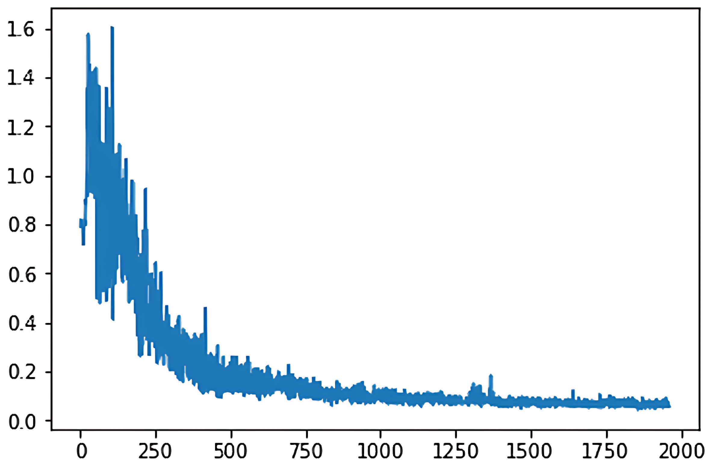
In the two different training models, the loss function diagram representing classical deep Q-learning is shown in Figure 3, while Figure 4 displays the loss function for the adaptive deep Q-learning algorithm proposed in this thesis. In these figures, the horizontal axis represents the number of game turns, and the vertical axis represents the average loss every 50 game turns.

By comparing the graphs, we observe that the adaptive deep Q-learning algorithm demonstrates a smaller loss function value and converges in fewer turns compared to the classical deep Q-learning algorithm. This indicates that the adaptive deep Q-learning algorithm has a faster convergence speed and better convergence effectiveness.

4.2.2. Cumulative Reward

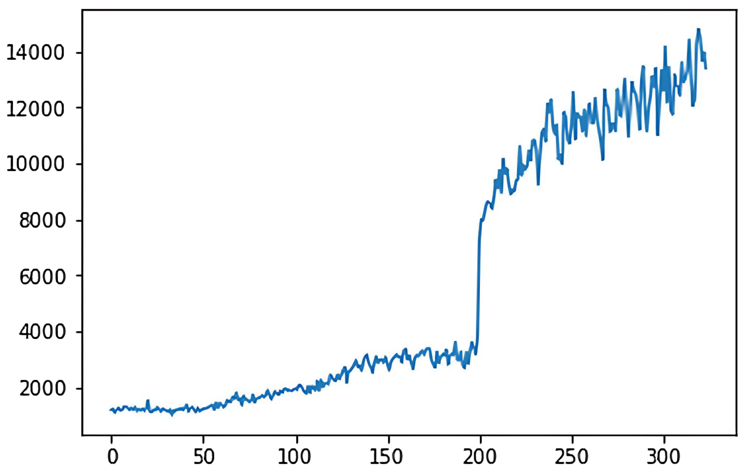
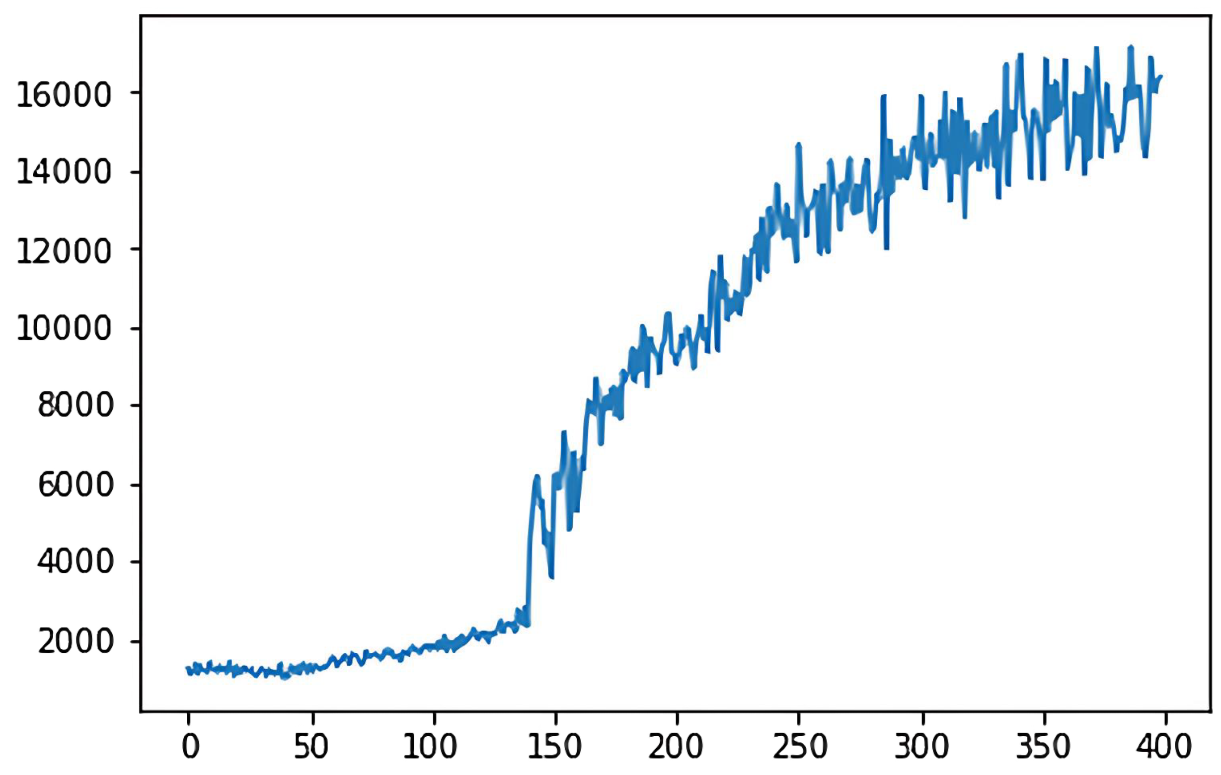
In the deep Q-learning algorithm, the cumulative reward value is the goal that the agent aims to maximize during the action selection process. The ultimate goal of the 2048 game is to synthesize the number 2048 or higher, which belongs to the category of maximizing reward or minimizing consumption, so the game’s goal belongs to the quantitative goals. For the quantitative goal, we use the cumulative reward value as the criterion to evaluate the model. The cumulative reward for the classical deep Q-learning algorithm is shown in Figure 5, while Figure 6 shows the cumulative reward for the adaptive deep Q-learning algorithm proposed in this thesis. In these figures, the horizontal axis represents the number of game rounds, and the vertical axis indicates the average cumulative reward every 50 rounds.

A comparison of the two reward function graphs reveals that the adaptive deep Q-learning algorithm model has a higher reward score and achieves faster cumulative reward improvement than the classical deep Q-learning algorithm. Clearly, the adaptive deep Q-learning algorithm model not only secures a higher reward score but also requires fewer turns for reward enhancement, indicating a more effective cumulative reward improvement.

4.2.3. Performance Evaluation

In order to validate the feasibility and reliability of the proposed method, we tested the training weights after completing the training process. A total of 1000 tests were conducted, with the maximum score achieved being 4096, corresponding to 59,724 points, and the achievement rate for reaching 2048 was 10%. The specific distribution of test results is shown in

Table 3. Distribution of test scores.

Final Number	Achieving Rate
4096	0.05%
2048	10%
1024	60%
512	95%
256	100%
128	100%
64	100%
32	100%
16	100%
8	100%
4	100%
2	100%

below.

Additionally, as a contrast, we invited 32 players to participate in the 2048 game, and their average score was 8024, with the vast majority of players only able to reach the number 512. Clearly, the results from the method proposed in this thesis far exceed those of real players, indicating that the model performs exceptionally well.

5. Conclusions

This paper explores scalable wireless video transmission utilizing energy capture technology, modeling wireless video transmission as a Markov decision process. We introduce reinforcement learning, deep learning, and other methods, as well as the large deviation principle from limit theory, to enhance our approach.

Firstly, the concept of the Markov decision process is introduced in this paper, and wireless video transmission is modeled as a Markov decision process in order to solve the video transmission problem by reinforcement learning. Secondly, convolutional neural networks in deep learning are used for feature extraction of input variables in order to prevent overfitting and reduce the number of hyperparameters. Specifically, we introduce dropout technology for multiple forward propagations and apply it to both the training process and the prediction process at the same time. We randomly sample the prediction distribution obtained from sampling, and the maximum value of the sampled data is the output value of the network. During model training, there will be continuous negative rewards, which are mainly caused by the following two reasons: one is due to an unreasonable network setting, and the other is due to incomplete training. In order to accurately judge the cause of continuous negative rewards, this thesis calculates and processes small probability events based on the principle of large deviations and obtains the boundary number of negative rewards that minimize the probability of misjudgment. This method can save training time, correct network parameters in time, and judge the cause of continuous negative rewards quickly and accurately. Finally, because the structure of the 2048 game is similar to that of the scalable wireless video transmission Markov decision process, in order to verify the feasibility and superiority of the proposed method, this paper simulates scalable wireless video transmission through the 2048 game. The experimental results demonstrate the feasibility and superiority of the proposed framework.

A key limitation lies in the absence of real-world wireless video transmission data for performance validation. The real-world wireless video transmission data would entail more data processing problems and emergencies, dynamic environmental factors, and heightened training difficulties. Future studies should address these aspects to strengthen the model’s applicability.