Dynamic Stepsize Techniques in DR-Submodular Maximization ^†

Abstract

The Diminishing-Return (DR)-submodular function maximization problem has garnered significant attention across various domains in recent years. Classic methods often employ continuous greedy or Frank–Wolfe approaches to tackle this problem; however, high iteration and subproblem solver complexity are typically required to control the approximation ratio effectively. In this paper, we introduce a strategy that employs a binary search to find the dynamic stepsize, integrating it into traditional algorithm frameworks to address problems with different constraint types. We demonstrate that algorithms using this dynamic stepsize strategy can achieve comparable approximation ratios to those using a fixed stepsize strategy. In the monotone case, the iteration complexity is $O\left({\parallel \nabla F\left(\mathbf{0}\right)\parallel }_1{ϵ}^{-1}\right)$, while in the non-monotone scenario, it is $O\left(n+{\parallel \nabla F\left(\mathbf{0}\right)\parallel }_1{ϵ}^{-1}\right)$, where F denotes the objective function. We then apply this strategy to solving stochastic DR-submodular function maximization problems, obtaining corresponding iteration complexity results in a high-probability form. Furthermore, theoretical examples as well as numerical experiments validate that this stepsize selection strategy outperforms the fixed stepsize strategy.

1. Introduction

The problem of maximizing DR-submodular functions, which generalizes set submodular functions to more general domains such as integer lattices and box regions in Euclidean spaces, has emerged as a prominent research topic in optimization. Set submodular functions inherently capture the diminishing returns property, where the marginal gain of adding an element to a set decreases as the set expands. DR-submodular functions extend this fundamental property to continuous and mixed-integer domains, enabling broader applications in machine learning, graph theory, economics, and operations research [1,2,3,4]. This extension not only addresses practical problems with continuous variables but also provides a unified framework for solving set submodular maximization through continuous relaxation techniques [5,6].

The problem of deterministic DR-submodular function maximization considered in this paper can be formally written as follows:

$$\begin{array}{c}\hfill \underset{x\in \mathcal{X}}{max}F\left(x\right),\end{array}$$

(1)

where the feasible set $\mathcal{X}\subseteq {[0,1]}^n$ is compact and convex, and $F:{[0,1]}^n\mapsto {\mathbb{R}}_{+}$ is a differentiable DR-submodular function. While this problem is generally NP-hard, under certain structural assumptions, approximation algorithms with constant approximation ratios can be developed. For unconstrained scenarios, Niazadeh et al. [7] established a tight ${\displaystyle \frac{1}{2}}$-approximation algorithm, aligning with classical results for unconstrained submodular maximization. In constrained settings, monotonicity plays a critical role: convex-constrained monotone DR-submodular maximization admits a $\left(1-{\displaystyle \frac{1}{e}}\right)$-approximation [1], whereas non-monotone cases under down-closed constraints achieve ${\displaystyle \frac{1}{e}}$-approximation [1] with recent improvements to $0.401$ [8]. For general convex constraints containing the origin, a ${\displaystyle \frac{1-{min}_{x\in \mathcal{X}}{\parallel x\parallel }_{\infty }}{4}}$-approximation guarantee is attainable [9,10,11].

While deterministic DR-submodular maximization has been extensively studied, practical scenarios often involve uncertainties where the objective function can only be accessed through stochastic evaluations. This motivates the investigation of stochastic DR-submodular maximization problems, which are typically formulated as follows:

$$\begin{array}{c}\hfill \underset{x\in \mathcal{X}}{max}F\left(x\right):={\mathbb{E}}_{\xi \sim \mathbb{P}}\left[f(x,\xi )\right],\end{array}$$

(2)

where the DR-submodular function $F:{[0,1]}^n\to {\mathbb{R}}_{+}$ is defined as the expectation of stochastic functions $f(x,\xi ):{[0,1]}^n\times \Xi \to {\mathbb{R}}_{+}$ with $\xi \sim \mathbb{P}$. Building upon the Lyapunov framework established for deterministic problems [10], recent works like [12,13] have developed stochastic variants of continuous greedy algorithms. Specifically, Lian et al. [14] proposed SPIDER-based methods that reduce gradient evaluation complexity from $O\left({ϵ}^{-3}\right)$ in earlier works [12] to $O\left({ϵ}^{-2}\right)$ through variance reduction techniques.

The Lyapunov framework proposed by Du et al. [9,10] provides a unified perspective for analyzing DR-submodular maximization algorithms. By modeling algorithms as discretizations of ordinary differential equations (ODEs) in the time domain $[0, 1]$, this approach establishes a direct connection between continuous-time dynamics and discrete-time implementations. Specifically, the approximation ratio of discrete algorithms differs from their continuous counterparts by a residual term that diminishes as the stepsize approaches zero. However, the use of constant stepsizes in this framework imposes fundamental limitations: the required number of iterations grows inversely with stepsize magnitude, leading to linear computational complexity both in theory and practical implementations.

To address the limitations of fixed stepsize strategies, recent advances have explored dynamic stepsize adaptation for submodular optimization. For box-constrained DR-submodular maximization, Chen et al. [15] developed a ${\displaystyle \frac{1}{2}}$-approximation algorithm with $\mathcal{O}(1/ϵ)$ adaptive rounds, where stepsizes are selected through enumeration over a candidate set of size $\mathcal{O}(log1/ϵ)$. Furthermore, Ene et al. [16] achieved ${\displaystyle \frac{1}{e}}$-approximation for non-monotone cases using $\mathcal{O}\left(log{\displaystyle \frac{n}{ϵ}}log{\displaystyle \frac{1}{ϵ}}log{\displaystyle \frac{2n+m}{{ϵ}^2}}\right)$ parallel rounds, and $(1-{\displaystyle \frac{1}{e}})$-approximation for monotone cases with $\mathcal{O}\left(log{\displaystyle \frac{n}{ϵ}}log{\displaystyle \frac{m+n}{{ϵ}^2}}\right)$ rounds. These works inspire our development of binary search-based dynamic stepsizes that achieve comparable approximation guarantees while reducing computational complexity.

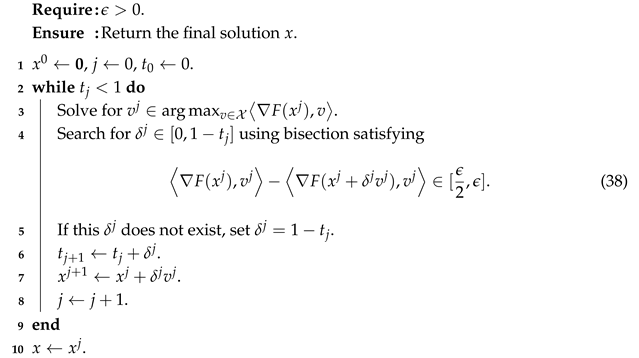
The dynamic stepsize strategy in this paper leverages binary search to approximate solutions to univariate equations by selecting intervals based on midpoint function value signs, ensuring convergence via monotonicity and continuity. While stochastic methods like simulated annealing [17] address non-convex/stochastic problems via probabilistic criteria, their guarantees depend on cooling schedules and lack deterministic convergence. In contrast, our binary search framework exploits the monotonicity/continuity of the stepsize equation (Equation (38)), achieving sufficiently precise solutions with guaranteed efficiency, avoiding cooling parameter dependencies and focusing on theoretical foundations for DR-submodular structures.

1.1. Contributions

This paper introduces a novel dynamic stepsize strategy for DR-submodular maximization problems, offering significant improvements over traditional fixed stepsize methods. Our approach achieves state-of-the-art approximation guarantees while reducing computational complexity. Notably, the iteration complexity of our algorithms is independent of the smoothness parameter L. In the monotone case, it is also independent of the variable dimension n. Furthermore, both the gradient evaluation complexity and function evaluation complexity exhibit only a logarithmic dependence on the problem dimension n and the smoothness parameter L. Below, we summarize the key contributions:

• Deterministic DR-Submodular Maximization: For deterministic settings, our dynamic stepsize strategy achieves the following complexity bounds:

  –

  In the monotone case, the iteration complexity is $O\left({\displaystyle \frac{{\parallel \nabla F\left(\mathbf{0}\right)\parallel }_1}{ϵ}}\right)$, where ${\parallel \nabla F\left(\mathbf{0}\right)\parallel }_1$ reflects the gradient norm at the origin, and $ϵ$ denotes the discretization error.

  –

  For non-monotone functions, the iteration complexity increases to $O\left(n+{\displaystyle \frac{{\parallel \nabla F\left(\mathbf{0}\right)\parallel }_1}{ϵ}}\right)$, accounting for the added challenge posed by non-monotonicity.

  To determine the stepsize dynamically, we employ a binary search procedure, introducing an additional factor of $O\left(log{\displaystyle \frac{nL}{ϵ}}\right)$ to the evaluation complexity.
• Stochastic DR-Submodular Maximization: Extending our approach to stochastic settings, we achieve comparable complexity results with high probability:

  –

  For monotone objective functions, the iteration complexity remains $O\left({\displaystyle \frac{{\parallel \nabla F\left(\mathbf{0}\right)\parallel }_1}{ϵ}}\right)$.

  –

  In the non-monotone case, the complexity is $O\left(n+{\displaystyle \frac{{\parallel \nabla F\left(\mathbf{0}\right)\parallel }_1}{ϵ}}\right)$.

  These results demonstrate that our method maintains efficiency regardless of the smoothness parameter L, making it particularly suitable for large-scale stochastic optimization problems.
• Empirical Validation: We validate the effectiveness of our dynamic stepsize strategy through three examples: multilinear extensions of set submodular functions, DR-submodular quadratic functions, and softmax extensions for determinantal point processes (DPPs). The results confirm that our approach outperforms fixed stepsize strategies in terms of both iteration complexity and practical performance.

Table 1. Algorithms and theoretical guarantees in this paper. D = Deterministic; S = Stochastic; M = Monotone; NM = Non-Monotone; DC = Down-closed; GC = General convex; Grad Eval = Gradient evaluation complexity; S-Grad Eval = Single (per-sample) gradient evaluation complexity.

Algorithm	Setting	Complexity	Approximation Ratio
Algorithm 2	D-M/GC	Iter: $O\left({\displaystyle \frac{{\parallel \nabla F\left(0\right)\parallel }_1}{ϵ}}\right)$	$1-1/e$ (Theorem 2)
		Grad eval: $O\left({\displaystyle \frac{{\parallel \nabla F\left(0\right)\parallel }_1}{ϵ}}log{\displaystyle \frac{nL}{ϵ}}\right)$
Algorithm 3	D-NM/DC	Iter: $O\left(n+{\displaystyle \frac{{\parallel \nabla F\left(0\right)\parallel }_1}{ϵ}}\right)$	${\displaystyle \frac{1}{e}}$ (Theorem 3)
		Grad eval: $O\left(\left(n+{\displaystyle \frac{{\parallel \nabla F\left(0\right)\parallel }_1}{ϵ}}\right)log{\displaystyle \frac{nL}{ϵ}}\right)$
Algorithm 4	D-NM/GC	Iter: $O\left(n+{\displaystyle \frac{{\parallel \nabla F\left(0\right)\parallel }_1}{ϵ}}\right)$	${\displaystyle \frac{1}{4}}$ (Theorem 4)
		Grad eval: $O\left(\left(n+{\displaystyle \frac{{\parallel \nabla F\left(0\right)\parallel }_1}{ϵ}}\right)log{\displaystyle \frac{nL}{ϵ}}\right)$
Algorithm 5	S-M/GC	Oracle: $O\left({\displaystyle \frac{{\parallel \nabla F\left(0\right)\parallel }_1}{ϵ}}\right)$	$1-1/e$ (Theorem 5)
		S-Grad eval: $O\left({\displaystyle \frac{{\parallel \nabla F\left(\mathbf{0}\right)\parallel }_1}{{ϵ}^4}}·log{\displaystyle \frac{nL}{{ϵ}^2}}·log{\displaystyle \frac{{\parallel \nabla F\left(\mathbf{0}\right)\parallel }_1}{ϵ\sigma }}\right)$
Algorithm 6	S-NM/DC	Oracle: $O\left(n+{\displaystyle \frac{{\parallel \nabla F\left(0\right)\parallel }_1}{ϵ}}\right)$	${\displaystyle \frac{1}{e}}$ (Theorem 6)
		S-Grad eval: $O\left({ϵ}^{-3}\left({\displaystyle \frac{{\parallel \nabla F\left(\mathbf{0}\right)\parallel }_1}{ϵ}}+n\right)·log{\displaystyle \frac{nL}{{ϵ}^2}}·log{\displaystyle \frac{{\parallel \nabla F\left(\mathbf{0}\right)\parallel }_1}{ϵ\sigma }}\right)$
Algorithm 7	S-NM/GC	Oracle: $O\left(n+{\displaystyle \frac{{\parallel \nabla F\left(0\right)\parallel }_1}{ϵ}}\right)$	${\displaystyle \frac{1}{4}}$ (Theorem 7)
		S-Grad eval: $O\left({ϵ}^{-3}\left({\displaystyle \frac{{\parallel \nabla F\left(\mathbf{0}\right)\parallel }_1}{ϵ}}+n\right)·log{\displaystyle \frac{nL}{{ϵ}^2}}·log{\displaystyle \frac{{\parallel \nabla F\left(\mathbf{0}\right)\parallel }_1}{ϵ\sigma }}\right)$

provides a unified overview of our algorithms’ theoretical guarantees and computational complexities (iteration and gradient evaluation bounds) under diverse problem settings, enabling readers to rapidly grasp the efficiency and adaptability of our dynamic stepsize framework.

1.2. Organizations

The organization of the rest of this manuscript is as follows. Section 2 introduces the fundamental concepts and key results that form the basis of our work. In Section 3, we outline the design principles of our dynamic stepsize strategy and establish theoretical guarantees for both monotone and non-monotone deterministic objective functions. Section 4 extends our approach to stochastic settings, presenting algorithms and analyses tailored for monotone and non-monotone DR-submodular functions under uncertainty. In Section 5, we evaluate the computational efficiency of our strategy through its application to three canonical DR-submodular functions, with comprehensive numerical experiments validating the efficacy of the dynamic stepsize approach. Section 6 summarizes our key findings while discussing both limitations and promising future research directions.

2. Preliminaries

We begin by introducing the formal definition of a non-negative DR-submodular function defined on the continuous domain ${[0,1]}^n$, along with some fundamental properties.

Definition 1.

A function $F:{[0,1]}^n\to {\mathbb{R}}_{+}$ is said to be DR-submodular if for any two vectors $x,y\in {[0,1]}^n$ satisfying $x\le y$ (coordinate-wise) and any scalar $a\ge 0$ such that $x+a{e}_i, y+a{e}_i\in {[0,1]}^n$, the following inequality holds:

$$F(x+a{e}_i)-F\left(x\right)\ge F(y+a{e}_i)-F\left(y\right),$$

(3)

for all $i=1,\cdots ,n$. Here, $e_i$ represents the i-th standard basis vector in ${\mathbb{R}}^n$.

This property reflects the diminishing returns behavior of F along each coordinate direction. Specifically, the marginal gain of increasing a single coordinate diminishes as the input vector grows larger.

To facilitate further discussions, we introduce additional notation. Throughout this paper, the inequality $x\le y$ for two vectors means that $x_i\le y_i$ holds for all $i\in \left[n\right]$. Additionally, the operation $x\vee y$ is defined as ${(x\vee y)}_i=max\{x_i,y_i\}$, and $x\wedge y$ is defined as ${(x\wedge y)}_i=min\{x_i,y_i\}$.

An important result is that, in the differentiable case, DR-submodular functions are equivalent to the monotonic decrease in the gradient. Specifically, when F is differentiable, F is DR-submodular if and only if [2]

$$\nabla F\left(x\right)\ge \nabla F\left(y\right),\forall x\le y\in {[0,1]}^n.$$

(4)

Another essential property for differentiable DR-submodular functions that will be used in this paper is derived from the concavity-like behavior in non-negative directions, as stated in the following proposition.

Proposition 1

([18]). When F is differentiable and DR-submodular, then

$$\langle \nabla F\left(x\right),y-x\rangle \ge F(x\vee y)+F(x\wedge y)-2F\left(x\right),\forall x,y\in {[0,1]}^n.$$

(5)

In this paper, we also require the function F to be L-smooth, meaning that for any $x,y\in \mathcal{X}$, there holds

$$\parallel \nabla F\left(x\right)-\nabla F\left(y\right)\parallel \le L\parallel x-y\parallel ,$$

(6)

where $\parallel ·\parallel$ denotes the Euclidean norm unless otherwise specified. An important property of L-smooth functions is that they satisfy the following necessary (but not sufficient) condition:

$$F\left(y\right)-F\left(x\right)\ge \langle \nabla F\left(x\right),y-x\rangle -{\displaystyle \frac{L}{2}}{\parallel y-x\parallel }^2.$$

(7)

For the stochastic DR-submodular maximization problem (2), we introduce additional notations to describe the stochastic approximation of the objective function’s full gradient.

- At each iteration j, let ${\mathcal{M}}_j$ denote a random subset of samples drawn from $\mathbb{P}$, with m representing the size of ${\mathcal{M}}_j$.

- The stochastic gradient at x is computed as

$$\nabla f(x,{\mathcal{M}}_j):={\displaystyle \frac{1}{|{\mathcal{M}}_j|}}\sum _{\xi \in {\mathcal{M}}_j}\nabla f(x,\xi ).$$

(8)

- We use an unbiased estimator $h_j$ to approximate the true gradient $\nabla F\left(x^j\right)$.

All algorithms and theoretical analyses in this paper for problems (1) and (2) rely on the following foundational assumption:

Assumption 1.

The problems under consideration satisfy these conditions:

1. 

$F:{[0,1]}^n\to {\mathbb{R}}_{+}$ is DR-submodular and L-smooth.

2. 

$F\left(\mathbf{0}\right)=0$ and $\mathbf{0}\in \mathcal{X}$.

3. 

A Linear-Objective Optimization (LOO) oracle is available, providing solutions to

$$\underset{x\in \mathcal{X}}{max}{c}^{\top }x\forall c\in {\mathbb{R}}^n.$$

(9)

The following assumption is essential for the stochastic problem (2).

Assumption 2.

The stochastic gradient is unbiased—i.e.,

$$L_{\xi }[\nabla f(x,\xi )]=\nabla F\left(x\right).$$

(10)

This assumption ensures that the mini-batch gradient estimator $\nabla f(x,{\mathcal{M}}_j)$ satisfies

$$L_{{\mathcal{M}}_j}[\nabla f(x,{\mathcal{M}}_j)]=\nabla F\left(x\right),$$

(11)

where ${\mathcal{M}}_j$ denotes the random mini-batch sampled at iteration j. This property is critical for deriving high-probability guarantees in stochastic optimization.

Lyapunov Method for DR-Submodular Maximization

As discussed in [10], Lyapunov functions play a crucial role in the analysis of algorithms. Depending on the specific problem, the Lyapunov function can take various parametric forms. Taking the monotone DR-submodular maximization problem for example, the ideal algorithm can be designed as follows:

$$\begin{array}{ccc}\hfill v\left(x\right(t\left)\right)& \in & arg\underset{v\in \mathcal{X}}{max}\langle \nabla F\left(x\left(t\right)\right),v\rangle ,\hfill \\ \hfill \dot{x}\left(t\right)& =& v\left(x\right(t\left)\right).\hfill \end{array}$$

(12)

A unified parameterized form of the Lyapunov function is given by:

$$L\left(x\left(t\right)\right)=a_{t}F\left(x\left(t\right)\right)-b_{t}F\left(x\left(t\right)\right),t\in [0,T],$$

(13)

where $a_t$ and $b_t$ are time-dependent parameters.

The monotonicity of the Lyapunov function is closely tied to the approximation ratio of the algorithm, as demonstrated by the following inequality:

$$F\left(x\left(T\right)\right)\ge {\displaystyle \frac{b_T-b_0}{a_T}}F\left(x^{*}\right),$$

(14)

where $x^{*}$ represents the optimal solution. The specific values of $a_T$, $b_T$, and T depend on the problem under consideration and are chosen accordingly to achieve the desired theoretical guarantees. In this problem, letting $a_t=b_t=e^t,T=1$ can guarantee the monotonicity of $L\left(x\right(t\left)\right)$ and then the approximation ratio for monotone DR-submodular functions is:

$$F\left(x\left(1\right)\right)\ge \left(1-{\displaystyle \frac{1}{e}}\right)F\left(x^{*}\right).$$

(15)

For maximizing non-monotone DR-submodular functions with down-closed constraints, the ideal algorithm can be designed as follows:

$$\begin{array}{ccc}\hfill v\left(x\right(t\left)\right)& \in & arg\underset{v\in \mathcal{X}\cap \{v:v\le 1-x(t\left)\right\}}{max}\langle \nabla F\left(x\left(t\right)\right),v\rangle ,\hfill \end{array}$$

(16)

$$\begin{array}{ccc}\hfill \dot{x}\left(t\right)& =& {\alpha }_{t}v\left(x\left(t\right)\right).\hfill \end{array}$$

(17)

In this problem, let $a_t=e^t$, $b_t=t$, and $T=1$. Then the best approximation ratio for monotone DR-submodular functions is:

$$F\left(x\left(1\right)\right)\ge {\displaystyle \frac{1}{e}}F\left(x^{*}\right),$$

(18)

where $\mathcal{X}$ is down-closed.

For maximizing non-monotone DR-submodular functions with general convex constraints, the ideal algorithm can be designed as follows:

$$\begin{array}{ccc}\hfill v\left(x\right(t\left)\right)& \in & arg\underset{v\in \mathcal{X}}{max}\langle \nabla F\left(x\left(t\right)\right),v\rangle ,\hfill \end{array}$$

(19)

$$\begin{array}{ccc}\hfill \dot{x}\left(t\right)& =& {\alpha }_t[v\left(x\left(t\right)\right)-x\left(t\right)].\hfill \end{array}$$

(20)

In this problem, let $a_t={(t+1)}^2$, $b_t=t$, and $T=1$. Then the best approximation ratio for monotone DR-submodular functions is:

$$F\left(x\left(1\right)\right)\ge {\displaystyle \frac{1}{4}}F\left(x^{*}\right),$$

(21)

where $\mathcal{X}$ is only convex.

In this paper, we focus on the same algorithmic ODE forms as those discussed above. However, our key improvement lies in the discretization process. Specifically, we aim to enhance the iteration complexity by employing a dynamic stepsize strategy. This approach allows for more efficient approximations while maintaining the desired theoretical guarantees, thereby advancing the state-of-the-art in DR-submodular maximization algorithms.

3. Deterministic Scenarios

In this section, we discuss the dynamic stepsize algorithms for maximizing deterministic DR-submodular functions, considering two cases: monotone and non-monotone. The fixed stepsize versions of the algorithms discussed in this section already exist in the literature, as documented in [6,9,10].

3.1. Monotone Case

In this subsection, we discuss a dynamic stepsize algorithm designed to maximize a monotone DR-submodular function while ensuring an approximation guarantee. To better illustrate the strategy for selecting the stepsize, we first introduce an idealized algorithm that relies on an oracle capable of solving a univariate continuous monotone equation. Subsequently, we propose a practical and implementable version of the algorithm.

3.1.1. An Idealized Algorithm

The ideal version referred to above is depicted as Algorithm 1. Unlike the fixed stepsize approach used in [10] where ${\delta }_j\equiv {\displaystyle \frac{1}{K}}$, our algorithm determines the stepsize by solving Equation (22). In brief, the stepsize is selected to ensure that the directional derivatives along $v^j$ between successive iterations differ precisely by $ϵ$.    

Algorithm 1: Ideal CG

Before analyzing the computational complexity and approximation guarantees of Algorithm 1, we must verify the feasibility of its output.

Lemma 1.

Algorithm 1 outputs a solution satisfying $x\in \mathcal{X}$.

Proof. 

Note that

$$\begin{array}{c}\hfill x\left(1\right)=x\left(0\right)+\sum _j{\delta }^j{v}^j=\sum _j{\delta }^j{v}^j,\end{array}$$

(23)

and ${\sum }_j{\delta }^j={\sum }_j{t}_{j+1}-t_j=1$. By the feasibility of $v^j$ and the convexity of P, we can prove the conclusion.    □

The iteration complexity bound is established as follows.

Lemma 2.

The iteration number K of Algorithm 1 satisfies

$$K\le {\displaystyle \frac{min\left\{{\parallel \nabla F\left(\mathbf{0}\right)\parallel }_1,nL\right\}}{ϵ}}+2.$$

(24)

Proof. 

For $j=0,\dots ,K-2$, we have

$$\begin{array}{ccc}\hfill 〈\nabla F\left(x^j\right)-\nabla F\left(x^{j+1}\right),\mathbf{1}〉& \ge & 〈\nabla F\left(x^j\right)-\nabla F\left(x^{j+1}\right),v^j〉=ϵ.\hfill \end{array}$$

(25)

Summing up this inequality from $j=0$ to $K-2$ yields

$$\begin{array}{ccc}\hfill (K-2)ϵ& \le & \sum _{j=0}^{K-3}〈\nabla F\left(x^j\right)-\nabla F\left(x^{j+1}\right),\mathbf{1}〉\hfill \\ & =& 〈\nabla F\left(x^0\right)-\nabla F\left(x^{K-2}\right),\mathbf{1}〉.\hfill \end{array}$$

(26)

Noting that ${\parallel \nabla F\left(\mathbf{0}\right)\parallel }_1\ge 〈\nabla F\left(x^0\right)-\nabla F\left(x^{K-2}\right),\mathbf{1}〉$ by the monotonicity of F, we can conclude that $K\le {\displaystyle \frac{{\parallel \nabla F\left(\mathbf{0}\right)\parallel }_1}{ϵ}}+2$.

By the fact that F is L-smooth and DR-submodular, there holds

$$\langle \nabla F\left(x^0\right)-\nabla F\left(x^{K-2}\right),\mathbf{1}\rangle \le nL.$$

(27)

Combining these bounds completes the proof.    □

As outlined in [10], the iteration complexity of the Frank–Wolfe algorithm for DR-submodular maximization is $O\left({\displaystyle \frac{nL}{ϵ}}\right)$. We now present the approximation guarantee and complexity results for Algorithm 1.

Theorem 1.

Assume that F is monotone. Then Algorithm 1 returns a solution x satisfying

$$F\left(x\right)\ge (1-e^{-1})F\left(x^{*}\right)-ϵ,$$

where $x^{*}$ denotes the optimal solution, with iteration complexity given by Equation (24).

Proof. 

Define the potential function $L\left(j\right):\{0,\dots ,K-1\}\to \mathbb{R}$ as

$$\begin{array}{c}\hfill L\left(j\right)=e^{t_j}\left[F\left(x^j\right)-F\left(x^{*}\right)\right].\end{array}$$

(28)

For $j=0,\dots ,K-1$, there holds

$$\begin{array}{ccc}\hfill & & L\left(j+1\right)-L\left(j\right)\hfill \\ \hfill & =& e^{t_{j+1}}(F\left(x^{j+1}\right)-F\left(x^{*}\right))-e^{t_j}(F\left(x^j\right)-F\left(x^{*}\right))\hfill \\ \hfill & =& e^{t_{j+1}}\left(F\left(x^{j+1}\right)-F\left(x^j\right)\right)+\left(e^{t_{j+1}}-e^{t_j}\right)\left(F\left(x^j\right)-F\left(x^{*}\right)\right)\hfill \\ \hfill & =& e^{t_{j+1}}{\int }_0^{{\delta }^j}〈\nabla F(x^j+t{v}^j),v^j〉dt+\left(e^{t_{j+1}}-e^{t_j}\right)\left(F\left(x^j\right)-F\left(x^{*}\right)\right)\hfill \end{array}$$

$$\begin{array}{ccc}\hfill & \ge & e^{t_{j+1}}{\delta }^j\left[〈\nabla F\left(x^j\right),v^j〉-ϵ\right]+\left(e^{t_{j+1}}-e^{t_j}\right)\left(F\left(x^j\right)-F\left(x^{*}\right)\right)\hfill \end{array}$$

(29)

$$\begin{array}{ccc}\hfill & \ge & e^{t_{j+1}}{\delta }^j\left[〈\nabla F\left(x^j\right),x^{*}〉-ϵ\right]+\left(e^{t_{j+1}}-e^{t_j}\right)\left(F\left(x^j\right)-F\left(x^{*}\right)\right)\hfill \end{array}$$

(30)

$$\begin{array}{ccc}\hfill & \ge & e^{t_{j+1}}{\delta }^j\left[〈\nabla F\left(x^j\right),x^j\vee x^{*}-x^j〉-ϵ\right]+\left(e^{t_{j+1}}-e^{t_j}\right)\left(F\left(x^j\right)-F\left(x^{*}\right)\right)\hfill \end{array}$$

(31)

$$\begin{array}{ccc}\hfill & \ge & e^{t_{j+1}}{\delta }^j\left[F(x^j\vee x^{*})-F\left(x^j\right)-ϵ\right]+\left(e^{t_{j+1}}-e^{t_j}\right)\left(F\left(x^j\right)-F\left(x^{*}\right)\right)\hfill \end{array}$$

(32)

$$\begin{array}{ccc}\hfill & \ge & e^{t_{j+1}}{\delta }^j\left[F\left(x^{*}\right)-F\left(x^j\right)-ϵ\right]+\left(e^{t_{j+1}}-e^{t_j}\right)\left(F\left(x^j\right)-F\left(x^{*}\right)\right)\hfill \end{array}$$

(33)

$$\begin{array}{ccc}\hfill & =& -e^{t_{j+1}}{\delta }^jϵ+\left(e^{t_{j+1}}{\delta }^j-e^{t_{j+1}}+e^{t_j}\right)\left(F\left(x^{*}\right)-F\left(x^j\right)\right)\hfill \end{array}$$

$$\begin{array}{ccc}\hfill & \ge & -e^{t_{j+1}}{\delta }^jϵ,\hfill \end{array}$$

(34)

where (29) holds for the monotonicity of $\nabla F$, (30) holds for the definition of $v^j$, (31) and (33) holds by the monotonicity of F and (32) is by Proposition 1. Thus,

$$\begin{array}{ccc}\hfill L\left(K\right)-L\left(0\right)& =& \sum _{j=0}^{K-1}L\left(j+1\right)-L\left(j\right)\hfill \\ & \ge & \sum _{j=0}^{K-1}-e^{t_{j+1}}{\delta }^jϵ\ge -eϵ\sum _{j=0}^{K-1}{\delta }^j=-eϵ.\hfill \end{array}$$

(35)

Simultaneously, there holds

$$\begin{array}{ccc}\hfill L\left(K\right)-L\left(0\right)& =& e(F\left(x\right)-F\left(x^{*}\right))-(F\left(x^0\right)-F\left(x^{*}\right)).\hfill \end{array}$$

(36)

Thus, we finally have

$$\begin{array}{c}\hfill F\left(x\right)\ge (1-e^{-1})F\left(x^{*}\right)-ϵ.\end{array}$$

(37)

The proof is completed.    □

3.1.2. Algorithm with Binary Search

An oracle for solving Equation (22) exactly is not always feasible in general cases. To address this, we propose employing a binary search technique to compute an approximate solution. This approach preserves the approximation ratio achieved by Algorithm 1, leading to the development of Algorithm 2. The key distinction between these two algorithms lies in the determination of the stepsize ${\delta }^j$ at each iteration.

In Algorithm 2, we utilize the bisection method to compute a compensation parameter ${\delta }_j$ that satisfies condition (38). The implementation begins by initializing the search interval as $[0,t_j]$. At each iteration, we evaluate the left-hand side of (38) at the midpoint of the current interval and determine whether the value belongs to the right sub-interval. Depending on this evaluation, we systematically discard either the left or right half of the interval and repeat the process. The well-defined nature of this procedure is guaranteed by the monotonicity and continuity of the left-hand side expression with respect to ${\delta }^i$.

Algorithm 2: Bisection continuous-greedy

Following a similar analysis to that of Algorithm 1, the number of iterations K in the “while” loop of Algorithm 2 can also be bounded.

Corollary 1.

For Algorithm 2, the iteration number satisfies

$$K\le {\displaystyle \frac{2min\{\parallel \nabla F\left(\mathbf{0}\right){\parallel }_1,nL\}}{ϵ}}+2.$$

(39)

To analyze the gradient evaluation complexity of F, it is necessary to examine the number of binary search steps required in each iteration to determine the stepsize.

Lemma 3.

For each iteration $j\in \{0,\dots ,K-1\}$, the stepsize ${\delta }^j$ can be determined within at most $M=1+{log}_2\left({\displaystyle \frac{nL}{ϵ}}\right)$ binary search steps.

Proof. 

Let ${\delta }^{*}$ represent the exact solution to the equation

$$\varphi \left({\delta }^j\right):=\langle \nabla F\left(x^j\right),v^j\rangle -\langle \nabla F(x^j+{\delta }^j{v}^j),v^j\rangle -{\displaystyle \frac{ϵ}{2}}=0.$$

(40)

Due to the monotonicity and continuity of the univariate function $\varphi \left({\delta }^j\right)$, the binary search process can identify an interval of length $2^{-M}$ that contains ${\delta }^{*}$. Let ${\delta }^j$ denote the right endpoint of this interval. Consequently, we have

$$0\le {\delta }^j-{\delta }^{*}\le 2^{-M}\le {\displaystyle \frac{ϵ}{2nL}}.$$

(41)

By the L-smoothness property of F, it follows that

$$\begin{array}{cc}\hfill \left|\langle \nabla F(x^j+{\delta }^{*}{v}^j),v^j\rangle -\langle \nabla F(x^j+{\delta }^j{v}^j),v^j\rangle \right|& =\left|\langle \nabla F(x^j+{\delta }^{*}{v}^j)-\nabla F(x^j+{\delta }^j{v}^j),v^j\rangle \right|\hfill \end{array}$$

(42)

$$\begin{array}{cc}\hfill & \le L({\delta }^j-{\delta }^{*}){\parallel v^j\parallel }^2\hfill \end{array}$$

(43)

$$\begin{array}{cc}\hfill & \le L·{\displaystyle \frac{ϵ}{2nL}}·n\hfill \end{array}$$

(44)

$$\begin{array}{cc}\hfill & ={\displaystyle \frac{ϵ}{2}}.\hfill \end{array}$$

(45)

Thus, we obtain

$$\begin{array}{cc}\hfill \langle \nabla F\left(x^j\right),v^j\rangle -\langle \nabla F(x^j+{\delta }^j{v}^j),v^j\rangle & ={\displaystyle \frac{ϵ}{2}}+\langle \nabla F(x^j+{\delta }^{*}{v}^j),v^j\rangle -\langle \nabla F(x^j+{\delta }^j{v}^j),v^j\rangle \hfill \\ \hfill & \le ϵ.\hfill \end{array}$$

(46)

Additionally, by the monotonicity of $\nabla F$, we know

$$\langle \nabla F(x^j+{\delta }^{*}{v}^j),v^j\rangle \ge \langle \nabla F(x^j+{\delta }^j{v}^j),v^j\rangle .$$

(47)

Combining these results with the definition of ${\delta }^{*}$, the proof is completed.    □

The approximation guarantee and oracle complexity of Algorithm 2 can now be derived.

Theorem 2.

Assume F is monotone. Then, Algorithm 2 outputs a solution x satisfying

$$F\left(x\right)\ge (1-e^{-1})F\left(x^{*}\right)-ϵ.$$

(48)

The LOO oracle complexity is at most $O\left({\displaystyle \frac{{\parallel \nabla F\left(\mathbf{0}\right)\parallel }_1}{ϵ}}\right)$, and the gradient evaluation complexity is at most $O\left({\displaystyle \frac{{\parallel \nabla F\left(\mathbf{0}\right)\parallel }_1}{ϵ}}log{\displaystyle \frac{nL}{ϵ}}\right)$.

Proof. 

The complexities of the LOO oracle and gradient evaluations can be established using Corollary 1 and Lemma 3. We now focus on deriving the approximation ratio.

Recall the function $L\left(j\right)$ defined in (34). For $j=0,\dots ,K-1$, we have

$$\begin{array}{cc}\hfill L(j+1)-L\left(j\right)& =e^{t_{j+1}}{\int }_0^{{\delta }^j}\langle \nabla F(x^j+t{v}^j),v^j\rangle dt+\left(e^{t_{j+1}}-e^{t_j}\right)\left(F\left(x^j\right)-F\left(x^{*}\right)\right).\hfill \end{array}$$

(49)

From the structure of Algorithm 2, the DR-submodularity, and the monotonicity of F, it follows that

$$\begin{array}{cc}\hfill {\int }_0^{{\delta }^j}\langle \nabla F(x^j+t{v}^j),v^j\rangle dt& \ge {\int }_0^{{\delta }^j}\langle \nabla F(x^j+{\delta }^j{v}^j),v^j\rangle dt\hfill \end{array}$$

(50)

$$\begin{array}{cc}\hfill & \ge {\delta }^j\left[\langle \nabla F\left(x^j\right),v^j\rangle -ϵ\right]\hfill \end{array}$$

(51)

$$\begin{array}{cc}\hfill & \ge {\delta }^j\left[\langle \nabla F\left(x^j\right),x^{*}\rangle -ϵ\right]\hfill \end{array}$$

(52)

$$\begin{array}{cc}\hfill & \ge {\delta }^j\left[\langle \nabla F\left(x^j\right),x^j\vee x^{*}-x^j\rangle -ϵ\right]\hfill \end{array}$$

(53)

$$\begin{array}{cc}\hfill & \ge {\delta }^j\left[F(x^j\vee x^{*})-F\left(x^j\right)-ϵ\right]\hfill \end{array}$$

(54)

$$\begin{array}{cc}\hfill & \ge {\delta }^j\left[F\left(x^{*}\right)-F\left(x^j\right)-ϵ\right].\hfill \end{array}$$

(55)

Thus, we obtain

$$\begin{array}{cc}\hfill L(j+1)-L\left(j\right)& \ge e^{t_{j+1}}{\delta }^j\left[F\left(x^{*}\right)-F\left(x^j\right)-ϵ\right]+\left(e^{t_{j+1}}-e^{t_j}\right)\left(F\left(x^j\right)-F\left(x^{*}\right)\right)\hfill \end{array}$$

(56)

$$\begin{array}{cc}\hfill & =-e^{t_{j+1}}{\delta }^jϵ+\left(e^{t_{j+1}}{\delta }^j-e^{t_{j+1}}+e^{t_j}\right)\left(F\left(x^{*}\right)-F\left(x^j\right)\right)\hfill \end{array}$$

(57)

$$\begin{array}{cc}\hfill & \ge -e^{t_{j+1}}{\delta }^jϵ.\hfill \end{array}$$

(58)

Summing up these inequalities for $j=0$ to $K-1$, we obtain

$$\begin{array}{cc}\hfill L\left(K\right)-L\left(0\right)& =\sum _{j=0}^{K-1}\left(L(j+1)-L\left(j\right)\right)\hfill \end{array}$$

(59)

$$\begin{array}{cc}\hfill & \ge \sum _{j=0}^{K-1}-e^{t_{j+1}}{\delta }^jϵ\hfill \end{array}$$

(60)

$$\begin{array}{cc}\hfill & \ge -eϵ.\hfill \end{array}$$

(61)

On the other hand, by the definition of $L\left(j\right)$, we have

$$\begin{array}{cc}\hfill L\left(K\right)-L\left(0\right)& =e\left(F\left(x\right)-F\left(x^{*}\right)\right)-\left(F\left(\mathbf{0}\right)-F\left(x^{*}\right)\right)\hfill \end{array}$$

(62)

$$\begin{array}{cc}\hfill & =eF\left(x\right)+(1-e)F\left(x^{*}\right).\hfill \end{array}$$

(63)

Combining these results yields the approximation guarantee stated in the theorem.    □

3.2. Non-Monotone Case

In this subsection, we discuss the dynamic stepsize strategy for maximizing DR-submodular functions after removing monotonicity, along with its theoretical guarantees. Unlike the monotonic case, here we categorize the constraints into two types: down-closed and general convex types.

3.2.1. Down-Closed Constraint

Algorithm 3 is proposed for scenarios involving down-closed constraints, which means that if $x\in \mathcal{X}$ and $0\le y\le x$, then $y\in \mathcal{X}$. The fundamental framework is inspired by the measured continuous greedy (MCG) algorithm introduced in [6], initially raised for maximizing the multilinear extension relaxation of submodular set functions. In [10], MCG was demonstrated to require $O\left({\displaystyle \frac{nL}{ϵ}}\right)$ iterations to ensure an approximation loss of $ϵ$.

Algorithm 3: Bisection MCG

The feasibility of the output produced by Algorithm 3 is ensured by the down-closed property of $\mathcal{X}$.

Lemma 4.

The solution x generated by Algorithm 3 satisfies $x\in \mathcal{X}$.

The proof of is presented in Appendix A.

The absence of the monotonicity assumption for F necessitates a distinct analysis of the iteration complexity for Algorithm 3 compared to Algorithm 2.

Lemma 5.

For Algorithm 3, the number of iterations K satisfies

$$K\le min\left\{n+{\displaystyle \frac{{2\parallel \nabla F\left(\mathbf{0}\right)\parallel }_1}{ϵ}},{\displaystyle \frac{2nL}{ϵ}}\right\}+2.$$

(65)

Proof. 

The upper bound $K\le {\displaystyle \frac{2nL}{ϵ}}+2$ follows analogous reasoning to Corollary 1.

Note that at the $K-1$-th iteration of the algorithm, we have $\nabla F\left(x^{K-2}\right)\nleqq 0$—i.e., there exists at least one $i\in \left[n\right]$ such that ${\left.{\displaystyle \frac{\partial F}{\partial x_i}}\right|}_{x=x^{K-2}}>0$, or else we can let $v^j=\mathbf{0}$ and terminate the algorithm.

Now, consider the changing process of the sign of $\nabla F\left(x^j\right)$ for $j=0,\dots ,K-2$.

Case I. $\nabla F\left(x^{K-2}\right)\ge 0$. In this case, the analysis is analogous to that in Lemma 2 and we have

$$K\le {\displaystyle \frac{{\parallel \nabla F\left(\mathbf{0}\right)\parallel }_1}{ϵ}}+2\sim O\left({\displaystyle \frac{{\parallel \nabla F\left(\mathbf{0}\right)\parallel }_1}{ϵ}}\right).$$

(66)

Case II. $\nabla F\left(x^{K-2}\right)\ngeqq 0$. First, we define the iteration index set $S\subseteq [K-1]$ as the following:

$$S=\left\{j\in [K-1]:\exists i\in \left[n\right]\mathit{such}\mathit{that}{\left.{\displaystyle \frac{\partial F}{\partial x_i}}\right|}_{x=x^j}>0,{\left.{\displaystyle \frac{\partial F}{\partial x_i}}\right|}_{x=x^{j+1}}<0\right\}.$$

(67)

It is obvious that $\left|S\right|\le n$.

For $j\notin S$, by the monotonicity of $\nabla F$ w.r.t. K, we have

$$\begin{array}{ccc}\hfill 〈\nabla F{\left(x^j\right)}^{+},\mathbf{1}〉-〈\nabla F{\left(x^{j+1}\right)}^{+},\mathbf{1}〉& =& 〈\nabla F{\left(x^j\right)}^{+}-\nabla F{\left(x^{j+1}\right)}^{+},\mathbf{1}〉\hfill \\ & \ge & 〈\nabla F\left(x^j\right)-\nabla F\left(x^{j+1}\right),v^j〉\ge {\displaystyle \frac{ϵ}{2}},\hfill \end{array}$$

(68)

since $v^j$, $\nabla F\left(x^j\right)$ and $\nabla F\left(x^{j+1}\right)$ are entry-wisely of the same sign. By the monotonicity of $\nabla F\left(x\right)$, the number of these iterations can be bounded as

$$\begin{array}{ccc}\hfill {\parallel \nabla F\left(\mathbf{0}\right)\parallel }_1& \ge & {\parallel \nabla F\left(\mathbf{0}\right)}^{+}{\parallel }_1-{\parallel \nabla F{\left(x^{K-2}\right)}^{+}\parallel }_1\hfill \\ & =& \sum _{j=0}^{K-3}〈\nabla F{\left(x^j\right)}^{+},\mathbf{1}〉-〈\nabla F{\left(x^{j+1}\right)}^{+},\mathbf{1}〉\hfill \\ & \ge & \sum _{j\notin S}〈\nabla F{\left(x^j\right)}^{+},\mathbf{1}〉-〈\nabla F{\left(x^{j+1}\right)}^{+},\mathbf{1}〉\hfill \\ & \ge & \left|[K-2]\setminus S\right|·{\displaystyle \frac{ϵ}{2}}.\hfill \end{array}$$

The proof is completed.    □

Building upon the preceding analysis, we establish the following approximation guarantee and complexity results for Algorithm 3:

Theorem 3.

For any down-closed feasible set $\mathcal{X}\subseteq {[0,1]}^n$, Algorithm 3 produces a solution x satisfying $F\left(x\right)\ge e^{-1}F\left(x^{*}\right)-ϵ$ with LOO oracle calls bounded by

$$O\left(n+{ϵ}^{-1}{\parallel \nabla F\left(\mathbf{0}\right)\parallel }_1\right),$$

(69)

and gradient evaluations at most

$$O\left(\left(n+{ϵ}^{-1}{\parallel \nabla F\left(\mathbf{0}\right)\parallel }_1\right)log{\displaystyle \frac{nL}{ϵ}}\right).$$

(70)

Proof. 

Redefine the potential function as $L\left(j\right)=e^{t_j}F\left(x^j\right)-t_{j}F\left(x^{*}\right)$. Then, for $j=0,\dots K-1$, there holds

$$\begin{array}{ccc}& & L\left(j+1\right)-L\left(j\right)\hfill \\ \hfill & =& e^{t_{j+1}}F\left(x^{j+1}\right)-t_{j+1}F\left(x^{*}\right)-e^{t_j}F\left(x^j\right)+t_{j}F\left(x^{*}\right)\hfill \\ \hfill & =& e^{t_{j+1}}\left(F\left(x^{j+1}\right)-F\left(x^j\right)\right)+\left(e^{t_{j+1}}-e^{t_j}\right)F\left(x^j\right)-(t_{j+1}-t_j)F\left(x^{*}\right)\hfill \\ & =& e^{t_{j+1}}{\int }_0^{{\displaystyle \frac{{\delta }^j}{e^{{\delta }^j}}}}〈\nabla F\left(x^j\right)+t{v}^j,v^j〉dt+\left(e^{t_{j+1}}-e^{t_j}\right)F\left(x^j\right)-(t_{j+1}-t_j)F\left(x^{*}\right).\hfill \end{array}$$

(71)

Similar to the proof of Theorem 2, we need to prove a lower bound on the difference of function values between two adjacent iteration points when F is non-monotone:

$$\begin{array}{ccc}\hfill {\int }_0^{{\displaystyle \frac{{\delta }^j}{e^{{\delta }^j}}}}〈\nabla F\left(x^j\right)+t{v}^j,v^j〉dt& \ge & {\displaystyle \frac{{\delta }^j}{e^{{\delta }^j}}}\left[〈\nabla F\left(x^j\right),v^j〉-ϵ\right]\hfill \\ \hfill & \ge & {\displaystyle \frac{{\delta }^j}{e^{{\delta }^j}}}\left[〈\nabla F\left(x^j\right),x^j\vee x^{*}-x^j〉-ϵ\right]\hfill \\ \hfill & \ge & {\displaystyle \frac{{\delta }^j}{e^{{\delta }^j}}}\left[F\left(x^j\right)\vee x^{*})-F\left(x^j\right)-ϵ\right]\hfill \\ & \ge & {\displaystyle \frac{{\delta }^j}{e^{{\delta }^j}}}\left[(1-\parallel x^j{\parallel }_{\infty })F\left(x^{*}\right)-F\left(x^j\right)-ϵ\right],\hfill \end{array}$$

(72)

where the third inequality is due to Proposition 1 and the fourth inequality is by Lemma 3 in [1], which implies that the following inequality holds:

$$\begin{array}{ccc}\hfill F(x\vee x^{*})& \ge & \left(1-{\parallel x\parallel }_{\infty }\right)F\left(x^{*}\right)=\left(1-\underset{i=1}{\overset{n}{max}}{x}_i\left(t\right)\right)F\left(x^{*}\right),\hfill \end{array}$$

(73)

for $\forall x\in \mathcal{X}$. Additionally, for the upper bound on the ${\ell }_{\infty }$-norm of $x^j$, we have the following claim.    □

Claim 1.

For all the iteration points $x^j$, $j=0,\dots ,K$, of Algorithm 3, we have $\parallel x^j{\parallel }_{\infty }\le 1-e^{-t_j}$.

The claim can be proved by induction. First, note that $\parallel x^0\parallel =0\le 1-e^0$. Assume that $\parallel x^j{\parallel }_{\infty }\le 1-e^{-t_j}$ for some j, then the proof can be finished by showing that

$$\begin{array}{ccc}\hfill {\left(x^{j+1}\right)}_i& \le & {\displaystyle \frac{{\delta }^j}{e^{{\delta }^j}}}+\left(1-{\displaystyle \frac{{\delta }^j}{e^{{\delta }^j}}}\right){\left(x^j\right)}_i\hfill \\ \hfill & \le & {\displaystyle \frac{{\delta }^j}{e^{{\delta }^j}}}+\left(1-{\displaystyle \frac{{\delta }^j}{e^{{\delta }^j}}}\right)\left(1-e^{-t_j}\right)\hfill \\ & \le & 1-e^{-t_j-{\delta }^j}.\hfill \end{array}$$

(74)

So the above formula yields

$$\begin{array}{ccc}\hfill & & L\left(j+1\right)-L\left(j\right)\hfill \\ \hfill & \ge & e^{t_{j+1}}{\displaystyle \frac{{\delta }^j}{e^{{\delta }^j}}}\left[e^{-t_j}F\left(x^{*}\right)-F\left(x^j\right)-ϵ\right]+\left(e^{t_{j+1}}-e^{t_j}\right)F\left(x^j\right)-(t_{j+1}-t_j)F\left(x^{*}\right)\hfill \\ \hfill & =& -e^{t_{j+1}}{\displaystyle \frac{{\delta }^j}{e^{{\delta }^j}}}ϵ+(e^{t_{j+1}-t_j}{\displaystyle \frac{{\delta }^j}{e^{{\delta }^j}}}-{\delta }^j)F\left(x^{*}\right)+(e^{t_{j+1}}-e^{t_j}-e^{t_{j+1}}{\displaystyle \frac{{\delta }^j}{e^{{\delta }^j}}})F\left(x^j\right)\hfill \\ \hfill & =& -e^{t_j}{\delta }^jϵ+(e^{t_{j+1}}-e^{t_j}-e^{t_{j+1}}{\displaystyle \frac{{\delta }^j}{e^{{\delta }^j}}})F\left(x^j\right)\hfill \\ & \ge & -e^{t_{j+1}}{\displaystyle \frac{{\delta }^j}{e^{{\delta }^j}}}ϵ.\hfill \end{array}$$

(75)

By summing Equation (75) over j from 0 to $K-1$, we obtain

$$\begin{array}{ccc}\hfill L\left(K\right)-L\left(0\right)& \ge & \sum _{j=0}^{K-1}-e^{t_j}{\delta }^jϵ\hfill \\ & \ge & -eϵ\sum _{j=0}^{K-1}{\delta }^j=-eϵ.\hfill \end{array}$$

(76)

Together with the fact $L\left(K\right)-L\left(0\right)=eF\left(x\right)-F\left(x^{*}\right)$, we obtain the theorem.

3.2.2. General Convex Constraint

This section presents a Frank–Wolfe variant designed for maximizing non-monotone DR-submodular functions under general convex constraints, where stepsizes are determined through binary search operations on Equation (38). A key distinction from prior methods in [10] and earlier approaches lies in our iterative tracking protocol. Specifically, the method requires maintaining records of both parameter vectors and their corresponding function evaluations at each iteration. Upon completing the iteration sequence, the procedure outputs the stored point achieving maximum functional value, contrasting with traditional implementations that directly return the final computed iterate.

The feasibility and approximation characteristics of solution x generated by Algorithm 4 are formally established through the following analytical results.    

Algorithm 4: Bisection Frank-Wolfe

Lemma 6.

Algorithm 4 produces a feasible solution satisfying $x\in \mathcal{X}$.

The proof of is presented in Appendix B.

Theorem 4.

The solution of Algorithm 4 satisfies

$$F\left(x\right)\ge {\displaystyle \frac{1}{4}}F\left(x^{*}\right)-{\displaystyle \frac{ϵ}{2}}$$

(78)

with computational complexity characterized by $O\left(n+{ϵ}^{-1}{\parallel \nabla F\left(\mathbf{0}\right)\parallel }_1\right)$ LOO oracle calls and $O\left(\left(n+{ϵ}^{-1}{\parallel \nabla F\left(\mathbf{0}\right)\parallel }_1\right)log{\displaystyle \frac{nL}{ϵ}}\right)$ gradient evaluations.

The proof of is presented in Appendix C.

4. Stochastic DR-Submodular Function Maximization

This section investigates stochastic maximization of DR-submodular functions under two distinct settings. Section 4.1 focuses on the monotone case, establishing theoretical guarantees for constrained optimization. Building upon this foundation, Section 4.2 extends the analysis to non-monotone scenarios, addressing both down-closed constraints and generalized convex constraints. For the fixed stepsize implementations of stochastic DR-submodular maximization algorithms, we refer readers to [12,14].

4.1. Stochastic Monotone DR-Submodular Maximization

Algorithm 5 implements a SPIDER-CG framework for continuous monotone DR-submodular optimization, integrating binary search for adaptive stepsize selection. Our approach builds on the recursive gradient estimator from [14], where Lian et al. consider an gradient approximation $h_j$ of $\nabla F\left(x^j\right)$ by adding an unbiased estimator of $\nabla F\left(x^j\right)-\nabla F\left(x^{j-1}\right)$ to $h_{j-1}$, and $h_0$ is given as an unbiased estimator of $\nabla F\left(x^0\right)$. Building upon this variance-reduced foundation, we adopt the binary search method to find out a proper dynamic stepsize.    

Algorithm 5: Bisection Stochastic CG

We have the following theorem on the theoretical results of Algorithm 5.

Theorem 5.

Assume that F is monotone and set $m=O({ϵ}^{-3}log{\displaystyle \frac{{\parallel \nabla F\left(\mathbf{0}\right)\parallel }_1}{ϵ\sigma }})$. Under Assumption 2, Algorithm 5 outputs a solution x satisfying

$$\begin{array}{c}\hfill \mathbb{E}\left[F\left(x\right)\right]\ge (1-{\displaystyle \frac{1}{e}})F\left(x^{*}\right)-{\displaystyle \frac{ϵ}{1-ϵ}}.\end{array}$$

(79)

With probability $1-\sigma$, the LOO oracle complexity is bounded by $O\left({\displaystyle \frac{{\parallel \nabla F\left(\mathbf{0}\right)\parallel }_1}{ϵ}}\right)$ and the gradient evaluation complexity is bounded by

$$O\left({\displaystyle \frac{{\parallel \nabla F\left(\mathbf{0}\right)\parallel }_1}{{ϵ}^4}}·log{\displaystyle \frac{nL}{{ϵ}^2}}·log{\displaystyle \frac{{\parallel \nabla F\left(\mathbf{0}\right)\parallel }_1}{ϵ\sigma }}\right).$$

Proof. 

Firstly, we provide the proof of the complexity. For $j=0,\cdots ,K-2$, from the deterministic algorithm, we have

$$\begin{array}{ccc}\hfill \mathbb{E}\left[〈\nabla f(x^j,{\mathcal{M}}_j)-\nabla f(x^{j+1},{\mathcal{M}}_j),1〉\right]& =& 〈\nabla F\left(x^j\right)-\nabla F(x^j+1),1〉\hfill \\ \hfill & \ge & 〈\nabla F\left(x^j\right)-\nabla F\left(x^{j+1}\right),v^j〉\hfill \\ & =& \mathbb{E}\left[〈\nabla f(x^j,{\mathcal{M}}_j)-\nabla f(x^{j+1},{\mathcal{M}}_j),v^j〉\right].\hfill \end{array}$$

(80)

According to the Chernoff bounds, let $X_i=〈\nabla f(x^j,{\mathcal{M}}_j)-\nabla f(x^{j+1},{\mathcal{M}}_j),v^j〉$, $X={\displaystyle \frac{1}{m}}{\sum }_{j=0}^m{X}_i$, $\mu =〈\nabla F\left(x^j\right)-\nabla F\left(x^{j+1}\right),v^j〉$, satisfying

$$\begin{array}{c}\hfill P(X\le (1+ϵ)\mu )\ge 1-e^{-{\displaystyle \frac{{ϵ}^{2}m\mu }{3}}}\ge 1-e^{-{\displaystyle \frac{{ϵ}^{3}m}{6(1+ϵ)}}}.\end{array}$$

(81)

For each iteration, the probability of $\mu \ge {\displaystyle \frac{1}{1+ϵ}}·{\displaystyle \frac{ϵ}{2}}$ is at least $1-e^{-{\displaystyle \frac{{ϵ}^{3}m}{6(1+ϵ)}}}$. For all j, the following inequality holds with a high probability ${\left(1-e^{-{\displaystyle \frac{{ϵ}^{3}m}{6(1+ϵ)}}}\right)}^K$,

$$\begin{array}{ccc}\hfill \mathbb{E}\left[〈\nabla f(x^j,{\mathcal{M}}_j)-\nabla f(x^{j+1},{\mathcal{M}}_j),v^j〉\right]& \ge & {\displaystyle \frac{1}{1+ϵ}}·{\displaystyle \frac{ϵ}{2}}.\hfill \end{array}$$

(82)

Then

$$\begin{array}{ccc}\hfill 〈\nabla F\left(x^0\right)-\nabla F\left(x^{K-2}\right),1〉& =& \sum _{j=0}^{K-3}〈\nabla F\left(x^j\right)-\nabla F\left(x^{j+1}\right),1〉\hfill \\ \hfill & \ge & \sum _{j=0}^{K-3}\mathbb{E}\left[〈\nabla f(x^j,{\mathcal{M}}_j)-\nabla f(x^{j+1},{\mathcal{M}}_j),v^j〉\right]\hfill \\ & \ge & (K-2)·{\displaystyle \frac{1}{1+ϵ}}·{\displaystyle \frac{ϵ}{2}}.\hfill \end{array}$$

(83)

It is noteworthy that

$$\parallel \nabla F\left(x^0\right){\parallel }_1={\parallel \mathbb{E}[\nabla f(x^0,{\mathcal{M}}_j)]\parallel }_1\ge \mathbb{E}\left[〈\nabla f(x^0,{\mathcal{M}}_j)-\nabla f(x^{K-2},{\mathcal{M}}_j),1〉\right].$$

Then we can obtain

$$\begin{array}{c}\hfill {∥\mathbb{E}\left[\nabla f(x^0,{\mathcal{M}}_j)\right]∥}_1\ge (K-2)·{\displaystyle \frac{1}{1+ϵ}}·{\displaystyle \frac{ϵ}{2}},\end{array}$$

(84)

$$\begin{array}{c}\hfill K\le {\displaystyle \frac{2\parallel \nabla F\left(x^0\right){\parallel }_1(1+ϵ)}{ϵ}}+2.\end{array}$$

(85)

Then we can obtain the complexity $O\left({\displaystyle \frac{\parallel \nabla F\left(x^0\right){\parallel }_1}{ϵ}}\right)$ with probability ${\left(1-e^{-{\displaystyle \frac{{ϵ}^{3}m}{6(1+ϵ)}}}\right)}^K$. According to Taylor expansion, we have

$$\begin{array}{c}\hfill {\left(1-e^{-{\displaystyle \frac{{ϵ}^{3}m}{6(1+ϵ)}}}\right)}^K\ge 1-K·e^{-{\displaystyle \frac{{ϵ}^{3}m}{6(1+ϵ)}}}.\end{array}$$

(86)

Denote $\sigma :=K·e^{-{\displaystyle \frac{{ϵ}^{3}m}{6(1+ϵ)}}}$. The number m of set ${\mathcal{M}}_j$ is at most

$$6{ϵ}^{-3}(1+ϵ)log{\displaystyle \frac{2{ϵ}^{-1}{\parallel \nabla F\left(x^0\right)\parallel }_1(1+ϵ)+2}{\sigma }}.$$

Let

$$\begin{array}{ccc}\hfill \varphi \left({\delta }^j\right)& :=& 〈\nabla f(x^j,{\mathcal{M}}_j),v^j〉-〈\nabla f(x^j+{\delta }^j{v}^j,{\mathcal{M}}_j),v^j〉-{\displaystyle \frac{ϵ}{2}}.\hfill \end{array}$$

(87)

$$\begin{array}{c}\hfill \mathbb{E}\left[〈\nabla f(x^j,{\mathcal{M}}_j),v^j〉-〈\nabla f(x^j+{\delta }^{*}{v}^j,{\mathcal{M}}_j),v^j〉\right]={\displaystyle \frac{ϵ}{2}}.\end{array}$$

(88)

From the deterministic case, letting the right endpoint of the interval be ${\delta }^j$ yields

$$\begin{array}{c}\hfill 0\le {\delta }^j-{\delta }^{*}\le 2^{-M}\le \left(1-{\displaystyle \frac{1}{1+ϵ}}\right){\displaystyle \frac{ϵ}{2nL}}.\end{array}$$

(89)

From the above, for all j, there holds the following inequation in high probability.

$$\begin{array}{c}\hfill \mathbb{E}\left[〈\nabla f(x^j,{\mathcal{M}}_j),v^j〉\right]-\mathbb{E}\left[〈\nabla f(x^j+{\delta }^j{v}^j,{\mathcal{M}}_j),v^j〉\right]\ge {\displaystyle \frac{1}{1+ϵ}}·{\displaystyle \frac{ϵ}{2}}.\end{array}$$

(90)

Then

$$\begin{array}{ccc}\hfill & & \left|\mathbb{E}\left[〈\nabla f(x^j+{\delta }^j{v}^j,{\mathcal{M}}_j),v^j〉\right]-\mathbb{E}\left[〈\nabla f(x^j+{\delta }^{*}{v}^j,{\mathcal{M}}_j),v^j〉\right]\right|\hfill \\ \hfill & =& \left|\mathbb{E}\left[〈\nabla f(x^j+{\delta }^j{v}^j,{\mathcal{M}}_j)-\nabla f(x^j+{\delta }^{*}{v}^j,{\mathcal{M}}_j),v^j〉\right]\right|\hfill \\ \hfill & =& \left|〈\nabla F(x^j+{\delta }^j{v}^j,{\mathcal{M}}_j)-\nabla F(x^j+{\delta }^{*}{v}^j,{\mathcal{M}}_j),v^j〉\right|\hfill \\ & \le & L({\delta }^j-{\delta }^{*}){\parallel v^j\parallel }^2\le \left(1-{\displaystyle \frac{1}{1+ϵ}}\right)·{\displaystyle \frac{ϵ}{2}}.\hfill \end{array}$$

(91)

Now, we focus on the approximation ratio. Define the function $L\left(j\right)$ as

$$\begin{array}{c}\hfill L\left(j\right):=e^{t_j}\left(\mathbb{E}\left[F\left(x^j\right)\right]-F\left(x^{*}\right)\right).\end{array}$$

(92)

For $j=0,\dots K-1$, there holds

$$\begin{array}{c}\hfill L\left(j+1\right)-L\left(j\right)=e^{t_{j+1}}\mathbb{E}\left[{\int }_0^{{\delta }^j}〈\nabla F\left(x^j+t{v}^j\right),v^j〉dt\right]+\left(e^{t_{j+1}}-e^{t_j}\right)\left(\mathbb{E}\left[F\left(x^j\right)\right]-F\left(x^{*}\right)\right).\end{array}$$

(93)

By the form of Algorithm 5 and the DR-submodularity and monotonicity of F, we have

$$\begin{array}{ccc}\hfill & & \mathbb{E}\left[{\int }_0^{{\delta }^j}〈\nabla F\left(x^j+t{v}^j\right),v^j〉dt\right]\hfill \\ \hfill & \ge & \mathbb{E}\left[{\int }_0^{{\delta }^j}〈\nabla F\left(x^j+{\delta }^j{v}^j\right),v^j〉dt\right]\hfill \\ \hfill & \ge & \mathbb{E}\left[{\delta }^j〈\nabla F\left(x^j+{\delta }^j{v}^j\right),v^j〉\right]\hfill \\ \hfill & =& {\delta }^j\mathbb{E}\left[〈\mathbb{E}\left[h_{j+1}\right],v^j〉\right]\hfill \\ \hfill & =& {\delta }^j\mathbb{E}\left[〈\mathbb{E}\left[h_j+\nabla f\left(x^{j+1},{\mathcal{M}}_{j+1}\right)-\nabla f\left(x^j,{\mathcal{M}}_{j+1}\right)\right],v^j〉\right]\hfill \\ \hfill & =& {\delta }^j\mathbb{E}\left[〈\mathbb{E}\left[h_j\right],v^j〉+〈\mathbb{E}\left[\nabla f\left(x^{j+1},{\mathcal{M}}_{j+1}\right)-\nabla f\left(x^j,{\mathcal{M}}_{j+1}\right)\right],v^j〉\right]\hfill \\ \hfill & \ge & {\delta }^j\mathbb{E}\left[〈\mathbb{E}\left[h_j\right],x^j\vee x^{*}-x^j〉+〈\mathbb{E}\left[\nabla f\left(x^{j+1},{\mathcal{M}}_{j+1}\right)-\nabla f\left(x^j,{\mathcal{M}}_{j+1}\right)\right],v^j〉\right]\hfill \\ \hfill & =& {\delta }^j\mathbb{E}\left[〈\nabla F\left(x^j\right),x^j\vee x^{*}-x^j〉+〈\mathbb{E}\left[\nabla f\left(x^{j+1},{\mathcal{M}}_{j+1}\right)-\nabla f\left(x^j,{\mathcal{M}}_{j+1}\right)\right],v^j〉\right]\hfill \\ \hfill & \ge & {\delta }^j\mathbb{E}\left[F\left(x^j\vee x^{*}\right)-F\left(x^j\right)+〈\mathbb{E}\left[\nabla f\left(x^{j+1},{\mathcal{M}}_{j+1}\right)-\nabla f\left(x^j,{\mathcal{M}}_{j+1}\right)\right],v^j〉\right]\hfill \\ & \ge & {\delta }^j\mathbb{E}\left[F\left(x^{*}\right)-F\left(x^j\right)+〈\mathbb{E}\left[\nabla f\left(x^{j+1},{\mathcal{M}}_{j+1}\right)-\nabla f\left(x^j,{\mathcal{M}}_{j+1}\right)\right],v^j〉\right].\hfill \end{array}$$

(94)

Thus, we have

$$\begin{array}{ccc}\hfill & & L(j+1)-L\left(j\right)\hfill \end{array}$$

$$\begin{array}{ccc}& \ge & {\delta }^j{e}^{t_{j+1}}\mathbb{E}\left[F\left(x^{*}\right)-F\left(x^j\right)+〈\mathbb{E}\left[\nabla f\left(x^{j+1},{\mathcal{M}}_{j+1}\right)-\nabla f\left(x^j,{\mathcal{M}}_{j+1}\right)\right],v^j〉\right]\hfill \end{array}$$

(95)

$$\begin{array}{ccc}\hfill & & +\left(e^{t_{j+1}}-e^{t_j}\right)\left(\mathbb{E}\left[F\left(x^j\right)\right]-F\left(x^{*}\right)\right)\hfill \\ \hfill & \ge & {\delta }^j{e}^{t_{j+1}}\mathbb{E}\left[F\left(x^{*}\right)-F\left(x^j\right)-{\displaystyle \frac{ϵ}{1-ϵ}}\right]+\left(e^{t_{j+1}}-e^{t_j}\right)\left(\mathbb{E}\left[F\left(x^j\right)\right]-F\left(x^{*}\right)\right)\hfill \\ \hfill & =& \left({\delta }^j{e}^{t_{j+1}}-e^{t_{j+1}}+e^{t_j}\right)\left(F\left(x^{*}\right)-\mathbb{E}\left[F\left(x^j\right)\right]\right)-{\delta }^j{e}^{t_{j+1}}{\displaystyle \frac{ϵ}{1-ϵ}}\hfill \end{array}$$

$$\begin{array}{ccc}& \ge & -{\delta }^j{e}^{t_{j+1}}{\displaystyle \frac{ϵ}{1-ϵ}}.\hfill \end{array}$$

(96)

Summing up all the above inequalities from $j=0$ to $K-1$ yields

$$\begin{array}{ccc}\hfill L\left(K\right)-L\left(0\right)& =& \sum _{j=0}^{K-1}L(j+1)-L\left(j\right)\hfill \\ \hfill & \ge & \sum _{j=0}^{K-1}-{\delta }^j{e}^{t_{j+1}}{\displaystyle \frac{ϵ}{1-ϵ}}\hfill \\ & \ge & -e{\displaystyle \frac{ϵ}{1-ϵ}}.\hfill \end{array}$$

(97)

On the other hand, by the definition of function L, we have

$$\begin{array}{ccc}\hfill L\left(K\right)-L\left(0\right)& =& e\left(\mathbb{E}\left[F\left(x^K\right)\right]-F\left(x^{*}\right)\right)-\left(\mathbb{E}\left[F\left(\mathbf{0}\right)\right]-F\left(x^{*}\right)\right)\hfill \\ & =& e\mathbb{E}\left[F\left(x\right)\right]+\left(1-e\right)F\left(x^{*}\right).\hfill \end{array}$$

(98)

Then

$$\begin{array}{c}\hfill \mathbb{E}\left[F\left(x^K\right)\right]\ge \left(1-{\displaystyle \frac{1}{e}}\right)F\left(x^{*}\right)-{\displaystyle \frac{ϵ}{1-ϵ}}.\end{array}$$

(99)

   □

4.2. Stochastic Non-Monotone DR-Submodular Maximization

This subsection investigates the stochastic maximization of non-monotone DR-submodular functions under two constraint classes: down-closed convex sets and general convex domains.

4.2.1. Down-Closed Constraint

Algorithm 6 is designed for a stochastic non-monotone DR-submodular function with a down-closed constraint.    

Algorithm 6: Bisection Stochastic MCG

Theorem 6.

Assume that $\mathcal{X}\subseteq {[0,1]}^n$ is down-closed and set $m=O\left({ϵ}^{-3}log\left({\displaystyle \frac{{\parallel \nabla F\left(\mathbf{0}\right)\parallel }_1}{ϵ\sigma }}+{\displaystyle \frac{n}{\sigma }}\right)\right)$. Under Assumption 2, Algorithm 6 outputs a solution x satisfying

$$\begin{array}{c}\hfill \mathbb{E}\left[F\left(x\right)\right]\ge e^{-1}F\left(x^{*}\right)-ϵ.\end{array}$$

(101)

With probability $1-\sigma$, the LOO oracle complexity is bounded by $O\left({\displaystyle \frac{{\parallel \nabla F\left(\mathbf{0}\right)\parallel }_1}{ϵ}}+n\right)$ and the gradient evaluation complexity is bounded by

$$O\left({ϵ}^{-3}\left({\displaystyle \frac{{\parallel \nabla F\left(\mathbf{0}\right)\parallel }_1}{ϵ}}+n\right)·log{\displaystyle \frac{nL}{{ϵ}^2}}·log{\displaystyle \frac{{\parallel \nabla F\left(\mathbf{0}\right)\parallel }_1}{ϵ\sigma }}\right).$$

(102)

The proof of is presented in Appendix D.

4.2.2. General Convex Constraint

In this subsection, we present the dynamic stepsize algorithm for solving the maximization of stochastic non-monotone DR-submodular functions with general convex constraints.

Theorem 7.

Algorithm 7 outputs a solution x satisfying

$$\begin{array}{c}\hfill \mathbb{E}\left[F\left(x\right)\right]\ge {\displaystyle \frac{1}{4}}F\left(x^{*}\right)-{\displaystyle \frac{ϵ}{2}}.\end{array}$$

(103)

With probability $1-\sigma$, the LOO oracle complexity is bounded by $O\left({\displaystyle \frac{{\parallel \nabla F\left(0\right)\parallel }_1}{ϵ}}+n\right)$ and the gradient evaluation complexity is bounded by $O\left({ϵ}^{-3}\left({\displaystyle \frac{{\parallel \nabla F\left(0\right)\parallel }_1}{ϵ}}+n\right)·log{\displaystyle \frac{nL}{{ϵ}^2}}·log{\displaystyle \frac{\parallel \nabla F\left(x^0\right){\parallel }_1}{ϵ\sigma }}\right)$.

The proof of is presented in Appendix E.

Algorithm 7: Bisection Stochastic Frank–Wolfe

5. Examples

To explore the potential acceleration offered by a dynamic stepsize strategy, we present three illustrative examples in this section.

Multilinear Relaxation for Submodular Maximization. Let V be a finite ground set, and let $f:2^V\to \mathbb{R}$ be a function. The multilinear extension of f is defined as

$$\begin{array}{c}\hfill F\left(x\right)=\sum _{S\subseteq V}f\left(S\right)\prod _{i\in S}{x}_i\prod _{i\notin S}(1-x_i),\end{array}$$

(105)

where $x\in {[0,1]}^{\left|V\right|}$. It is well known that the function f is submodular (i.e., $f(S\cap \{e\left\}\right)-f\left(S\right)\ge f(T\cap \{e\left\}\right)-f\left(T\right)$ for any $S\subseteq T\subseteq V$ and $e\notin T$) if and only if F is DR-submodular. Therefore, maximizing a submodular function f can be achieved by first solving the maximization of its multilinear extension and then obtaining a feasible solution to the original problem through a rounding method. Such algorithms are known to provide strong approximation guarantees [5,19].

Let $e_i$ denote the vector whose i-th entry is 1 and all other entries are 0. The upper bound of ${\parallel \nabla F\left(\mathbf{0}\right)\parallel }_1$ can be derived as follows.

Lemma 7.

Let F denote of a submodular set function f. Suppose the feasible set $\mathcal{X}$ satisfies $\mathcal{X}\supseteq {\left\{e_i\right\}}_{i=1}^n$ and we have

$${\parallel \nabla F\left(\mathbf{0}\right)\parallel }_1\le nF\left(x^{*}\right).$$

(106)

For the multilinear extension of a submodular set function, the Lipschitz constant L is given by $L=O\left(n^2\right)F\left(x^{*}\right)$ [6].

Softmax Relaxation for DPP MAP Problem. Determinantal point processes (DPPs) are probabilistic models that emphasize diversity by capturing repulsive interactions, making them highly valuable in machine learning for tasks requiring varied selections. Let H denote the positive semi-definite kernel matrix associated with a DPP. The softmax extension of the DPP maximum a posteriori (MAP) problem is expressed as

$$\begin{array}{c}\hfill F\left(x\right)=\log \det \left(\mathrm{diag}\left(x\right)(H-I)+I\right),x\in {[0,1]}^n,\end{array}$$

(107)

where I represents the identity matrix. Based on Corollary 2 in [4], the gradient of the softmax extension $F\left(x\right)$ can be written as follows:

$$\begin{array}{c}\hfill {\nabla }_{i}F\left(x\right)={\left({(\mathrm{diag}\left(x\right)(H-I)+I)}^{-1}(H-I)\right)}_{ii},\forall i\in \left[n\right].\end{array}$$

(108)

Consequently, the ${\ell }_1$-norm of the gradient at $\mathbf{0}$ is given by

$${\parallel \nabla F\left(\mathbf{0}\right)\parallel }_1=\sum _{i=1}^n|H_{ii}-1|.$$

(109)

In practical scenarios involving DPPs, the matrix H is often a Gram matrix, where the diagonal elements $H_{ii}$ are universally bounded. This implies that the asymptotic growth of ${\parallel \nabla F\left(\mathbf{0}\right)\parallel }_1$ is upper-bounded by $O\left(n\right)$.

DR-Submodular Quadratic Functions. Consider a quadratic function $F\left(x\right)$ of the form

$$\begin{array}{c}\hfill F\left(x\right)={\displaystyle \frac{1}{2}}{x}^{T}Ax+a^{T}x+c,\end{array}$$

(110)

where $A\in {\mathbb{R}}_{-}^{n\times n}$ (i.e., A is a matrix with non-positive entries). In this case, $F\left(x\right)$ is DR-submodular. It is straightforward to verify that ${\parallel \nabla F\left(\mathbf{0}\right)\parallel }_1={\parallel a\parallel }_1\le n,$ and the gradient Lipschitz constant is given by $L={\parallel A\parallel }_2.$

The computational complexities of the algorithms designed to address the three constrained DR-submodular function maximization problems outlined earlier are compiled in

Table 2. Comparison of complexities between dynamic and constant stepsizes for three examples (grad.eval: complexity of gradient evaluation).

Examples	Dynamic Stepsize		Constant Stepsize
	LOO	grad.eval	LOO (grad.eval)
MLE	$O\left({\displaystyle \frac{n}{ϵ}}\right)$	$O({\displaystyle \frac{n}{ϵ}}log{\displaystyle \frac{n}{ϵ}})$	$O\left({\displaystyle \frac{n^3}{ϵ}}\right)$
Softmax	$O\left({\displaystyle \frac{n}{ϵ}}\right)$	$O({\displaystyle \frac{n}{ϵ}}log{\displaystyle \frac{nL}{ϵ}})$	$O\left({\displaystyle \frac{nL}{ϵ}}\right)$
Quadratic	$O\left({\displaystyle \frac{{\left|\right|a\left|\right|}_1}{ϵ}}\right)$	$O({\displaystyle \frac{{\left|\right|a\left|\right|}_1}{ϵ}}log{\displaystyle \frac{{n\left|\right|A\left|\right|}_2}{ϵ}})$	$O\left({\displaystyle \frac{{n\left|\right|A\left|\right|}_2}{ϵ}}\right)$

. The results presented in the table reveal that the dynamic stepsize strategy introduced in this work offers a significant advantage in terms of complexity over the constant stepsize approach, both for the MLE and softmax relaxation problems. However, in the quadratic case, a definitive comparison of their complexities cannot be made, because they are determined by the ${\ell }_1$-norm of the linear term vector and the ${\ell }_2$-norm of the quadratic term matrix, respectively, and there is no inherent relationship between the magnitudes of these two quantities.

Numerical Experiments

We conduct numerical experiments to evaluate different stepsize selection strategies for solving DR-submodular maximization problems. Our investigation focuses on two fundamental classes of objective functions: quadratic DR-submodular functions and softmax extension functions. The experimental framework builds upon established methodologies from [9,14], with necessary adaptations for our specific analysis.

Our experimental evaluation considers two problem classes: softmax extension problems and quadratic DR-submodular problems with linear constraints. Since neither problem class inherently satisfies monotonicity, we augment both functions with an additional $b^{T}x$ term, where b is a positive vector with components in appropriate ranges. This modification enables the verification of Algorithms 2 and 5 by ensuring monotonicity preservation.

We evaluate Algorithms 2–4 on the softmax extension problems, while testing the stochastic algorithms (Algorithms 5–7) on quadratic DR-submodular problems with incorporated random variables. The randomization methodology follows the principled approach outlined in [14].

For each problem class, we consider decision space dimensions $n\in \{40,100\}$, with the number of constraints m set as $0.5n$ for each dimension. The approximation parameter $ϵ$ is fixed at 0.1, and the constant stepsize strategy employs 100 iterations. Each configuration is executed with five independent trials, with averaged results reported.

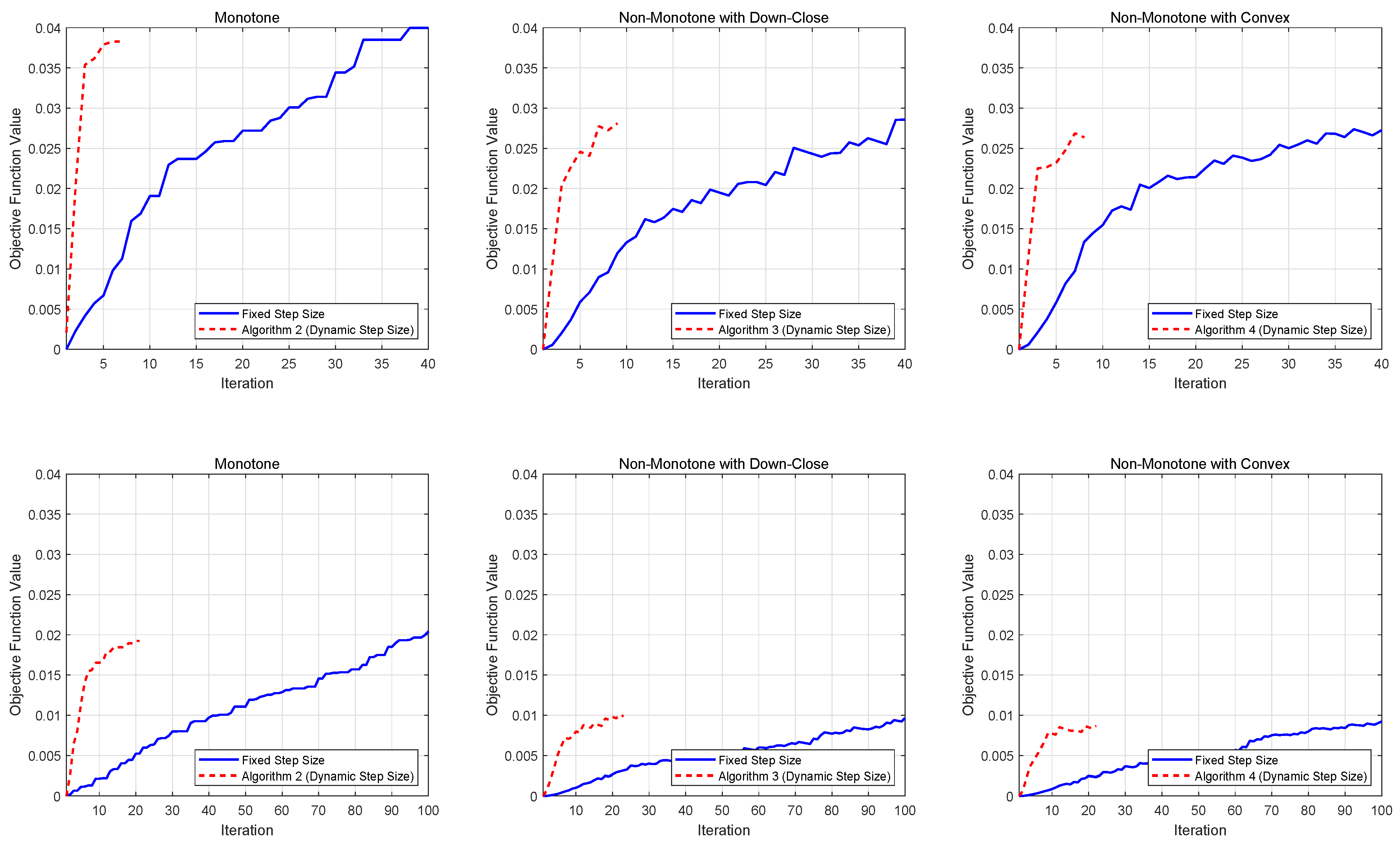
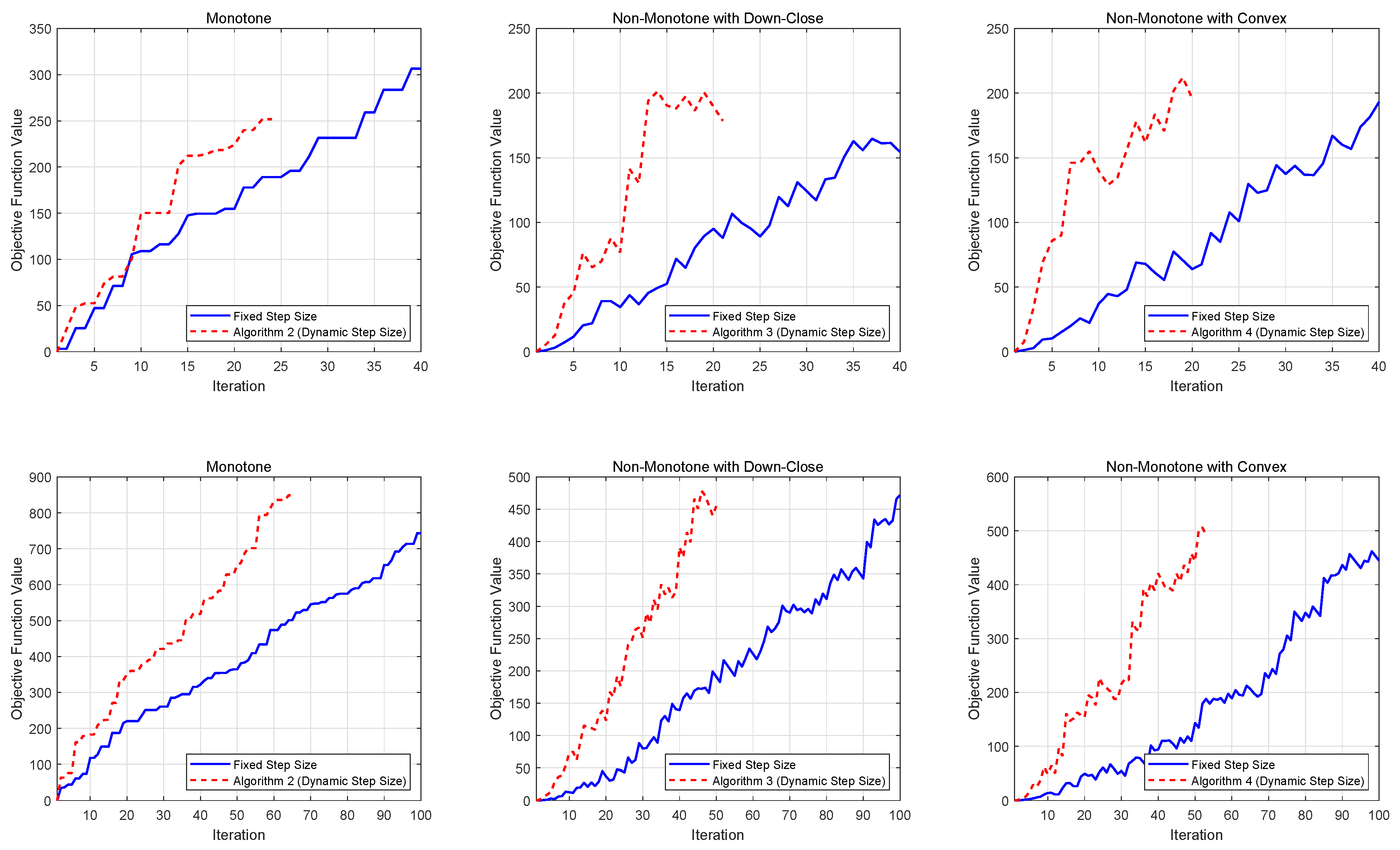
Figure 1 presents the performance comparison for softmax extension problems, while Figure 2 displays the results for stochastic quadratic DR-submodular problems. Both figures demonstrate the evolution of achieved function values across different stepsize strategies, providing empirical insights into algorithmic efficiency.

From the numerical results, we observe that for both deterministic and stochastic problems, dynamic stepsizes generally lead to lower iteration complexity compared to constant stepsizes, especially for larger problem dimensions. This finding highlights the advantages of using dynamic stepsizes in solving DR-submodular maximization problems.

6. Conclusions

This paper introduces a dynamic stepsize strategy for DR-submodular maximization, achieving iteration complexities independent of the smoothness parameter L. In deterministic settings, monotone cases attain $(1-1/e)$-approximation with $O\left({\displaystyle \frac{{\parallel \nabla F\left(0\right)\parallel }_1}{ϵ}}\right)$ iterations, while non-monotone problems under down-closed or general convex constraints achieve $1/e$ and $1/4$-approximations with $O\left(n+{\displaystyle \frac{{\parallel \nabla F\left(0\right)\parallel }_1}{ϵ}}\right)$ iterations. For stochastic optimization, variance reduction techniques (e.g., SPIDER) further reduce gradient evaluation complexities while maintaining high-probability guarantees. Empirical results on multilinear extensions, DPP softmax relaxations, and DR-submodular quadratics validate the practical efficiency of our methods compared to fixed stepsize baselines.

Our work has three key limitations: first, while our dynamic strategy matches the iteration complexity of fixed stepsize methods, it does not guarantee superiority for all L-smooth DR-submodular functions. Second, Algorithm 1 avoids the L-smoothness assumption but requires a univariate equation oracle to solve Equation (22), which lacks practical applications as no real-world examples have been identified to support this assumption. Third, our stepsize mechanism heavily relies on the DR-submodularity property, limiting its applicability to non-DR-submodular functions or mixed-integer domains. These limitations highlight opportunities for future research to extend our framework to broader function classes and practical scenarios.

References

1. Bian, A.; Levy, K.; Krause, A.; Buhmann, J.M. Continuous DR-submodular maximization: Structure and algorithms. In Proceedings of the Advances in Neural Information Processing Systems, Long Beach, CA, USA, 4–9 December 2017; pp. 486–496. [Google Scholar]
2. Bian, A.A.; Mirzasoleiman, B.; Buhmann, J.; Krause, A. Guaranteed non-convex optimization: Submodular maximization over continuous domains. In Proceedings of the 20th International Conference on Artificial Intelligence and Statistics, PMLR 2017, Fort Lauderdale, FL, USA, 20–22 April 2017; pp. 111–120. [Google Scholar]
3. Bian, Y.; Buhmann, J.M.; Krause, A. Continuous submodular function maximization. arXiv 2020, arXiv:2006.13474. [Google Scholar]
4. Gillenwater, J.; Kulesza, A.; Taskar, B. Near-Optimal MAP Inference for Determinantal Point Processes. In Proceedings of the 25th International Conference on Neural Information Processing Systems, NIPS’12, Lake Tahoe, NV, USA, 3–6 December 2012; Curran Associates Inc.: Red Hook, NY, USA, 2012; Volume 2, pp. 2735–2743. [Google Scholar]
5. Calinescu, G.; Chekuri, C.; Pál, M.; Vondrák, J. Maximizing a monotone submodular function subject to a matroid constraint. SIAM J. Comput. 2011, 40, 1740–1766. [Google Scholar] [CrossRef]
6. Feldman, M.; Naor, J.; Schwartz, R. A unified continuous greedy algorithm for submodular maximization. In Proceedings of the 2011 IEEE 52nd Annual Symposium on Foundations of Computer Science, FOCS ’11, Palm Springs, CA, USA, 22–25 October 2011; IEEE Computer Society: Washington, DC, USA, 2011; pp. 570–579. [Google Scholar]
7. Niazadeh, R.; Roughgarden, T.; Wang, J.R. Optimal Algorithms for Continuous Non-Monotone Submodular and DR-Submodular Maximization. J. Mach. Learn. Res. 2020, 21, 1–31. [Google Scholar]
8. Buchbinder, N.; Feldman, M. Constrained submodular maximization via new bounds for dr-submodular functions. In Proceedings of the 56th Annual ACM Symposium on Theory of Computing, Vancouver, BC, Canada, 24–28 June 2024; Association for Computing Machinery: New York, NY, USA, 2024; pp. 1820–1831. [Google Scholar]
9. Du, D.; Liu, Z.; Wu, C.; Xu, D.; Zhou, Y. An improved approximation algorithm for maximizing a DR-submodular function over a convex set. arXiv 2022, arXiv:2203.14740. [Google Scholar]
10. Du, D. Lyapunov function approach for approximation algorithm design and analysis: With applications in submodular maximization. arXiv 2022, arXiv:2205.12442. [Google Scholar]
11. Mualem, L.; Feldman, M. Resolving the Approximability of Offline and Online Non-Monotone DR-Submodular Maximization over General Convex Sets. In Proceedings of the International Conference on Artificial Intelligence and Statistics, PMLR, Valencia, Spain, 25–27 April 2023; pp. 2542–2564. [Google Scholar]
12. Mokhtari, A.; Hassani, H.; Karbasi, A. Stochastic Conditional Gradient Methods: From Convex Minimization to Submodular Maximization. arXiv 2018, arXiv:1804.09554. [Google Scholar]
13. Hassani, H.; Karbasi, A.; Mokhtari, A.; Shen, Z. Stochastic Conditional Gradient++: (Non)Convex Minimization and Continuous Submodular Maximization. SIAM J. Optim. 2020, 30, 3315–3344. [Google Scholar] [CrossRef]
14. Lian, Y.; Xu, D.; Du, D.; Zhou, Y. A Stochastic Non-Monotone DR-Submodular Maximization Problem over a Convex Set. In Proceedings of the Computing and Combinatorics: 28th International Conference, COCOON 2022, Shenzhen, China, 22–24 October 2022; Springer Nature: Berlin/Heidelberg, Germany, 2023; Volume 13595, pp. 1–11. [Google Scholar]
15. Chen, L.; Feldman, M.; Karbasi, A. Unconstrained submodular maximization with constant adaptive complexity. In Proceedings of the 51st Annual ACM SIGACT Symposium on Theory of Computing, Phoenix, AZ, USA, 23–26 June 2019; Association for Computing Machinery: New York, NY, USA, 2019; pp. 102–113. [Google Scholar]
16. Ene, A.; Nguyen, H. Parallel algorithm for non-monotone DR-submodular maximization. In Proceedings of the International Conference on Machine Learning, PMLR, Virtual, 13–18 July 2020; pp. 2902–2911. [Google Scholar]
17. Delahaye, D.; Chaimatanan, S.; Mongeau, M. Simulated annealing: From basics to applications. In Handbook of Metaheuristics; Springer: Berlin/Heidelberg, Germany, 2018; pp. 1–35. [Google Scholar]
18. Hassani, H.; Soltanolkotabi, M.; Karbasi, A. Gradient Methods for Submodular Maximization. In Proceedings of the 31st International Conference on Neural Information Processing Systems, Long Beach, CA, USA, 4–9 December 2017; Curran Associates, Inc.: Red Hook, NY, USA, 2017; Volume 30, pp. 5843–5853. [Google Scholar]
19. Chekuri, C.; Vondrák, J.; Zenklusen, R. Submodular Function Maximization via the Multilinear Relaxation and Contention Resolution Schemes. SIAM J. Comput. 2014, 43, 1831–1879. [Google Scholar] [CrossRef]
Figure 1. Numerical results for softmax problems.
Mathematics 13 01447 g001
Figure 2. Numerical results for stochastic quadratic DR-submodular problems.
Mathematics 13 01447 g002