Abstract
Reinforcement learning models often rely on uncertainty estimation to guide decision-making in dynamic environments. However, the role of memory limitations in representing statistical regularities in the environment is less understood. This study investigated how limited memory capacity influence uncertainty estimation, potentially leading to misestimations of outcomes and environmental statistics. We developed a computational model incorporating active working memory processes and lateral inhibition to demonstrate how relevant information is selected, stored, and used to estimate uncertainty. The model allows for the detection of contextual changes by estimating expected uncertainty and perceived volatility. Two experiments were conducted to investigate limitations in information availability and uncertainty estimation. The first experiment explored the effect of cognitive load on memory reliance for uncertainty estimation. The results show that cognitive load diminished reliance on memory, lowered expected uncertainty, and increased perceptions of environmental volatility. The second experiment assessed how outcome exposure conditions affect the ability to detect environmental changes, revealing differences in the mechanisms used for environmental change detection. The findings emphasize the importance of memory constraints in uncertainty estimation, highlighting how misestimation of uncertainties is influenced by individual experiences and the capacity of working memory (WM) to store relevant information. These insights contribute to understanding the role of WM in decision-making under uncertainty and provide a framework for exploring the dynamics of reinforcement learning in memory-limited systems.
MSC:
91E40
1. Introduction
As we make daily choices, we learn to associate specific responses to unique stimuli with positive or negative outcomes, forming stimulus–response–outcome (SRO) contingencies essential for decision-making [1,2,3]. These decisions often rely on estimating probabilities of outcomes based on recent experiences [2], despite outcome uncertainties that can vary across repetitions. Humans track the value of choices by comparing recent and distant past reward estimates [4], supporting behavioral adaptation, especially in tasks requiring exploration or exploitation, based on prospection of future outcomes. This process involves dual learning to estimate both outcome value and outcome variability. Outcome variability or uncertainty in outcomes can be formalized as a probability distribution, quantified through higher-order moments like variance and skewness [5], with fluctuations in past outcomes increasing uncertainty and prompting dynamic belief updates [6].
Decision-making in such uncertain environments hinges on managing expected and unexpected uncertainty [7]. Expected uncertainty arises from known outcome variability, such as unreliable reward cues, where the SRO contingency may not reliably predict outcomes [8]. Learning agents address this by reducing learning rates [9], using meta-learning to minimize surprise from prediction errors [6] and relying on past events to estimate outcomes under established variability. In contrast, unexpected uncertainty [7] arises when large prediction errors invalidate learned SRO contingencies, which is often triggered when top-down predictions are contradicted by sensory data, forcing a modification of prior beliefs [1]. In volatile environments, where reward structures or outcome rules change frequently, higher unexpected uncertainty triggers rapid belief updates [9,10,11], often implemented through a fast learning rate to constantly update the SRO contingency [6,12,13]. Adaptive learning agents address this computational demand by adjusting their learning rates to align with environmental statistics [7,11,14]: slow updates and relying on distant past events during high expected uncertainty when the environment is considered stable, while shifting reliance to more recent outcomes in the presence of high unexpected uncertainty, prompts a significant reevaluation of value and potentially leads to behavioral changes [1].
To accommodate both expected and unexpected sources of uncertainty, computational models have become increasingly flexible in how they support learning. Classical models such as the Rescorla–Wagner model [15] and the Pearce–Hall model [8,16] update outcome estimates based on the discrepancy between predicted and actual outcomes, with the Pearce–Hall model improving adaptability by modulating learning rates in response to surprise. Surprise can be quantified relative to expected uncertainty through the computation of outcome variance, unsigned reward prediction errors, or even dynamic learning rates resulting from tracking the slope of errors over trials [17]. Likewise, ideal learning models, such as those based on Bayesian reasoning, can integrate prior knowledge with reward feedback using parameters like dynamic reward probabilities and distribution widths to estimate both expected and unexpected uncertainty [8,18,19]. Similarly, Kalman filter-based models adjust beliefs when prior’s uncertainty exceeds observation reliability [8,20]. However, these optimal models often overlook human cognitive constraints, particularly working memory (WM) limitations that impair adaptive learning and contribute to individual variability in uncertainty estimation [8,21].
Reinforcement learning models show that WM engagement reduces reward prediction error’s effect on outcome estimation [22,23], with the RLWM model [22] proposing a competition between reinforcement learning and capacity-limited WM systems. Study from Shibata et al. [24] showed that aligning WM representations with reinforcement learning task rules enhances learning, highlighting WM’s role in supporting reinforcement learning. Tavoni et al. [25] showed that reliance on WM decreased with higher volatility in dynamic conditions, and the need for frequent updates lessened with greater noise. Additional models like the Prediction of Responses and Outcomes (PRO) model [26,27] and the Hierarchical Error Representation (HER) model [28,29] incorporates WM to model serial error-correcting processes in learning, separately computing surprise and prediction error representations to modulate behavior adaptation.
In addition, Hassanzadeh et al. [30] demonstrated that incorporating forgetting and decay in WM representation reveals how WM dynamically interacts with visuomotor and reinforcement learning, emphasizing its contribution to adaptive cognition declines with age and cognitive impairment. Limited memory capacity in WM can impact adaptive belief updating by influencing the (mis)estimation of both expected and unexpected uncertainty. Expected uncertainty, tied to the spread of the outcome distribution, depends on memories of past outcomes. Unexpected uncertainty, associated with volatility [7], diminishes the influence of distant memories. When memory is constrained, environmental statistics may be misrepresented, leading to inaccurate uncertainty estimation. For instance, if memory samples do not fully reflect the true outcome distribution, expected uncertainty may not match the actual spread of the outcome distribution. In some cases, individual differences in uncertainty estimation can be attributed to differences in memory samples, even when exposed to the same outcomes under limited memory resources [31]. For example, overestimating expected uncertainty can decrease sensitivity to recent events, slowing adaptation or causing important changes to be overlooked; while underestimating expected uncertainty may amplify the influence of recent events, misinterpreting randomness as meaningful changes, resulting in unstable beliefs [31]. Moreover, Browning et al. [32] found that individuals with low trait anxiety adapted their learning rates to environmental volatility, while those with high trait anxiety struggled to do so. Misestimating uncertainty can hinder the ability to accurately track a dynamic environment, impairing decision-making and reducing the likelihood of optimal outcomes.
WM-based learning models, while addressing information handling, often do not fully explain how multiple pieces of information are selected. In HER [28,29], each WM module stores a single item, while RLWM [22] stores information that is subject to forgetting. Our focus is on how relevant information is held and updated in working memory, as task-relevant WM representations are key to understanding responses to uncertainty in reinforcement learning. Information gating mechanisms are central to WM-based learning, determining which observations are retained or suppressed based on action context [21,33]. Corticostriatal circuits enable flexible gating and updating of WM representations [34], allowing WM to prioritize relevant information until its utility diminishes [21,33,35]. Thus, gating is crucial for modulating learning rates in both stable and volatile environments, where maintaining or discarding prior outcomes can shape outcome estimation.
The present study investigated how individual differences in WM capacity for withholding information influence choice history and prediction error in outcome estimation, encompassing the potential misestimation of uncertainty. It was hypothesized that WM capacity influences expected uncertainty, affecting how accurately individuals perceive surprise, noise, and volatility in the environment. While many reinforcement learning models address capacity limits through fixed memory storage constraints, this study developed a computational model with a WM gating mechanism for uncertainty estimation, providing a framework to better understand WM’s dynamic role in reinforcement learning and uncertainty estimation beyond fixed limits. The model explored how WM gates relevant information based on recency and utility, with utility increasing alongside informativeness and recency where higher-utility information replaced less relevant items in WM.
Along with the model, two human experiments were run to investigate how WM gating of outcomes affects uncertainty computation within the constraints of limited memory capacity. The study aimed to demonstrate the connection between WM load and uncertainty computation, a link that has been suggested in previous research but has not been clearly shown until now. The study hypothesizes that high cognitive load, defined as the amount of mental effort required to process task-related information within the limited capacity of WM [36], occupies working memory, leaving less capacity to actively maintain or retrieve other task-relevant information. This may in turn lead to lower expected uncertainty and increased perceived volatility during outcome learning. As a result, outcomes were expected to be estimated with reduced memory reliance. Outcome exposure influenced change detection mechanisms, emphasizing the role of memory constraints in uncertainty estimation. These findings highlight how individual experiences and WM capacity shape uncertainty misestimation, contributing to our understanding of decision-making under uncertainty.
2. The Model
The study explored how uncertainty estimation helps represent dynamic environments within memory-limited systems. Rather than relying on single outcome estimates, uncertainty estimations use distributions to detect changes, with surprising outcomes prompting learning updates. However, limited memory resources can lead to misestimations that reduce adaptability. The findings highlighted the roles of surprise and recency: surprising information influences estimations more, while older outcomes lose relevance, illustrating how memory constraints, surprise, and recency interact to shape individual differences in adapting to changing environments.
2.1. Model Overview
The model, as illustrated in Figure 1, integrates features from both normative models and those with limited memory capacity, incorporating a WM gating mechanism for uncertainty estimation. Its primary contribution was to examine how (mis)estimations of uncertainty are formed using a selective set of past observations or outcomes () that are gated into WM with limited capacity.
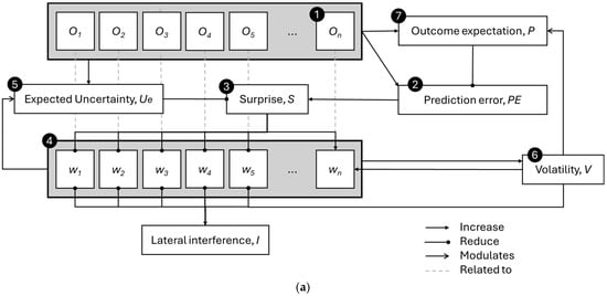
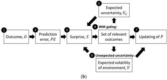
Figure 1.
(a) Graphical representation of the model for estimating uncertainty and facilitating learning, with different arrowhead styles indicating the type of effect: dot arrowheads represent a decreasing influence, pointed arrowhead type 1 indicates an increasing effect, and pointed arrowhead type 2 indicates activity modulation. (b) Flow diagram of the same computational process. The circled numbers represent different processes within the model, which will be detailed in the following subsections.
When a target is encountered, the model observes the outcome (1) and calculates the prediction error (2) by comparing the observed outcome with the expected one. The prediction error triggers the perception of surprise (3), which depends on the expected uncertainty of the outcome. The WM gating process (4) is influenced by the level of surprise from new observations, enhancing (or reducing) the gating-in of surprising outcomes and the gating-out of irrelevant previously stored outcomes. Since the model prioritizes outcomes with greater surprise, it suggests that the stored information reflects inconsistencies in the outcomes (i.e., valence). When holding more inconsistent memory traces of the target, the model introduces lateral inhibition of WM units, which increases the reduction in recalled outcome weights as more outcomes are stored (of an inconsistent nature). The lateral inhibition of outcome weights demonstrates how limited WM capacity may be regulated, facilitating the gating-out process. In addition, the gating mechanism is strengthened by higher perceived environmental volatility (6), which reflects the frequency of changes in the outcome structure. Based on the recalled outcomes for a target, the expected uncertainty (5) is formed. The model addressed the (mis)estimation of uncertainty by exploring variations in outcome recall (sampling) within WM. This also helps reduce the perception of surprise when the outcome falls within the expected distribution. Finally, the model updates the outcome expectation (7) if there is a significant deviation between the current expectation and the recalled outcomes, based on the likelihood of changes in the environment’s outcome structure.
2.2. Model Mechanism
2.2.1. Outcome Encounter
The model focuses on the outcomes of a single target. When the target is encountered, the most recent outcome (On) is registered into WM, depending on the weight (wn) associated with it.
2.2.2. Prediction Error and Surprise
Prediction error (PE) represents the signed difference between the current observed outcome (On) (i.e., rewards obtained) and the outcome prediction (P) or belief. PE is used to compute Surprise (S), as shown in Equation (1),
which was heuristically derived based on the Gaussian density formulation, using a scaled (through ) squared PE normalized by expected uncertainty (Ue) plus a stabilizing constant (a small value, e.g., 0.0001), transformed via an exponential function to ensure monotonicity and boundedness within the range of 0 (no surprise when PE = 0) to 1 (with high PE indicating an unexpected observation). Ue reduced surprise (S) when the prediction error (PE) was within the expected outcome distribution, while surprise increased when outcomes fell outside it. Figure 2 shows how surprise varied according to the different prediction errors and expected uncertainty when the outcome estimation was held constant.
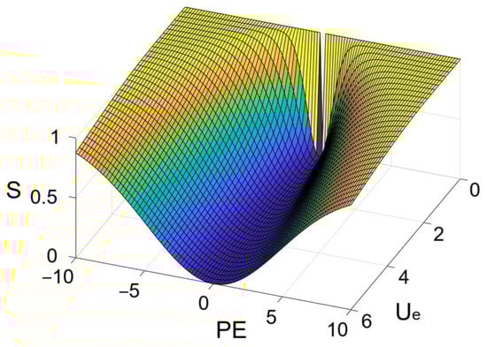
Figure 2.
An example showing the change in surprise according to PE and Ue when k1 = 8 and P = 0.
2.2.3. WM Gating Mechanism
The WM gating mechanism is incorporated in the model to manage the storage or removal of information in WM [21] for stimulus–outcome estimation and uncertainty. In each trial, the gating mechanism determined if a new observation (On) should be gated into WM and managed the relevance of stored information within limited capacity. When stored information became irrelevant, it was gated out. Both gating-in and gating-out were based on weights (w) assigned to each observed outcome (O), with outcomes with weights exceeding a fixed threshold (wt) retained in WM.
- WM gating-in mechanism:
The outcome weight wn ∈ [0, 1] is computed via a logistic function [37],
based on surprise (S) and perceived volatility (V), as follows:
where k2 is the base incremental gain used in the logistic function; k3 is the gain parameter associated with the volatility effect, which determines the slope of the function; #(w: w > wt) is the number of elements in w that is greater than the threshold (wt); k4 is the shift in the logistic function; and Vc ∈ [0, 1] is a free parameter that modulates the effect of surprise within the gating mechanism.
Surprise enhances salience, increasing the likelihood of an outcome entering working memory [38] by raising wn. A sharp rise in S signals unexpected uncertainty, especially in stable environments, and sustained high surprise may indicate a structural shift in outcome probabilities. The perceived volatility,
reflects how frequently the outcome structure changes. V increases with the number of perceived environmental changes (C) and decreases with the time since the last change (ti). To ensure that → 0 in the absence of changes, ti was initialized to a large value (e.g., 10,000). In volatile settings, the model favors new information over prior beliefs [39,40,41], capturing increased sensitivity to surprise and thus leading to higher wn for new outcomes. Moreover, when the WM holds few outcomes exceeding the gating threshold, greater weight is allocated to incoming outcomes, promoting their admission into working memory.
- WM maintenance and gating-out mechanism:
The WM gating mechanism prioritizes recent, high-utility outcomes to support future predictions, optimizing retrieval by balancing maintenance cost against expected future need [42]. Past outcome weights (w0: n−1) in WM are adjusted as follows:
where k5 is a free parameter modulating the impact of urge on w0: n-1, I represents the lateral inhibition, and urge represents the need to update beliefs (discussed in the next subsection). The attenuation of these weights is triggered by unexpected outcomes (via surprise) or environmental changes (via urge). Low surprise or urge reinforces stored outcomes, while high values reduce w0: n−1, reflecting diminished predictive value. The effect of urge emerged primarily when WM held sufficient outcomes. The influences of surprise, urge, and lateral inhibition (I) were modulated by volatility, increasing the likelihood of clearing irrelevant outcomes under high volatility. Lateral inhibition (I) limits recall when WM becomes overloaded [43]. As WM load increases, interference (weight reduction) through I rises, and retrieval increasingly favors recent, relevant outcomes. The decay of prior weights, coupled with the gating of “influential outcomes”, promotes a recency bias.
2.2.4. Expected Uncertainty
From the above, PE was scaled by the expected uncertainty (Ue) to compute surprise. While expected uncertainty is commonly quantified by outcome variance [1,5,44], variance is undefined for a new stimulus with a single observation. To address this, an initial bias term (H) was introduced in the estimation of Ue,
as a free parameter. As more outcomes are stored in WM, expected uncertainty transitioned from reliance on H to the variance in relevant stored outcomes (VarO), with the rate of transition controlled by a positive parameter k6. A low VarO indicates consistent, tightly clustered outcomes in WM, yielding lower expected uncertainty. Relevant outcomes are defined as those with weight exceeding the threshold.
With limited WM capacity, storing fewer outcomes can cause greater fluctuations in the variance in relevant outcomes (VarO), leading to over- or underestimation of expected uncertainty; overestimation reduces sensitivity to environmental changes, while underestimation increases susceptibility to noise, promoting false positives in change detection. Greater WM capacity allows better information storage and enables more stable variance estimates, aligning it more closely with the true outcome distribution.
2.2.5. Unexpected Uncertainty and Volatility
Stored outcomes in WM were cleared when a sudden rise in surprise or urge suppressed their influence, increasing the likelihood of removal and facilitating the gating-in of unexpected outcomes. Environmental changes were detected when urge, given by
exceeded a threshold, where k7 is the scaling factor that modulates the influence of the accumulated changes in variance estimates over time (. Urge was driven by recent outcome deviations and shifts in outcome variability, with the former quantified as the difference between the mean of relevant outcomes (MeanO) and the current prediction (P), scaled by expected uncertainty (Ue), and the latter by the accumulated changes in variance estimates over time ().
where k8 denotes the scaling factor for the variance threshold, with A and B representing the variance in the first and second halves of the stored outcomes exceeding outcome weight. The time range of stored outcomes reflects those still maintained in working memory, preserved in their order of encounter, provided that their context weights exceed the threshold.
Upon detecting an environmental change (i.e., urge exceeds threshold), Equation (5) updated perceived environmental changes (C) by incrementing it by 1 and resetting ti to the number of trials since the last detected change. Lastly, C∆var in Equation (9) was reset to 0.
2.2.6. Updating of Outcome Expectation
Expected outcomes were updated based on past hedonic values modeling the stimulus–outcome relationships. Both the WM-stored outcomes and uncertainty estimates influenced outcome expectation (P),
through the Rescorla–Wagner equation [15], with urge as the learning rate. This allows rapid updates of current outcome predictions toward the mean of relevant outcomes (MeanO) during high urge.
2.3. Model Fitting to Experiments
The model captures how WM gating and uncertainty estimation interact to represent environmental structure under capacity constraints. Outcome admission into WM is governed by a gating mechanism assigning weights based on surprise, volatility, and lateral inhibition. As WM load increases, lateral inhibition uniformly reduces weights, thus limiting capacity. High surprise outcomes initially receive greater weight, and despite gating-out decay, salient outcomes retain utility over time. With limited WM capacity, variance estimates become unstable, leading to misestimation of unexpected uncertainty and potential false detections of environmental change. Model parameters are listed in Appendix A Table A1.
The model was validated using two experiments examining how reliance on past outcomes shapes uncertainty estimation under cognitive demands. Experiment 1 tested how cognitive load impacts outcome estimation and perceived volatility, by requiring participants to track generative means under varying noise and volatility while under cognitive interference. This tested whether reduced WM availability impairs adaptive estimation and change detection, extending prior work [25]. Experiment 2 assessed sensitivity to changes in outcome distributions, testing how WM capacity and sample exposure influence detection of shift in mean or noise. Together, fitting the mode to these experiments evaluated its ability to capture how WM constraints shape individual difference in statistical learning [45,46], outcome estimation, and environmental change detection under cognitive demands.
3. Experiment I: How Working Memory Capacity Affects Uncertainty Misestimation
In uncertain environments, accurate estimation of expected uncertainty prevents overreaction to outcomes, but limited WM capacity causes individual differences in these estimations, even under identical outcome exposure. This experiment explored how WM capacity affects uncertainty estimation, particularly under cognitive load, where WM resources are shared across concurrent tasks, limiting information available for each of them. It was hypothesized that lower WM capacity would constrain information use during uncertainty estimation, especially under cognitive load, leading to underestimation of expected uncertainty and inflated perceived volatility when unexpected outcomes occur.
Participants completed a Gaussian Estimation Task (GET) to assess estimation accuracy across varying volatility and noise levels, with cognitive load (CLE) induced by a concurrent summation task. They also performed n-back tasks to assess WM, which required them to continuously update and maintain information while monitoring a sequence of stimuli and identify when the current stimulus matched the one presented n steps earlier. The model predicts that under cognitive load, individuals with lower WM capacity rely more on initial biases when estimating uncertainty, testing whether WM constraints impair adaptive uncertainty estimation and increase volatility misperception.
3.1. Participants
This experiment was run online as data collection occurred during the COVID-19 lockdown. A total of 66 participants were initially recruited from Prolific for the experiment. The experiment was conducted through Cognition.run, a framework for running behavioral experiments in a web browser. The data from the experiment was stored in Cognition.run. However, only 37 participants completed the tasks. Some of the participants who failed to complete the task decided to leave the experiment after the briefing on experiment instructions, while others had incomplete data stored in Cognition.run. Moreover, 10 participants from the 37 who had completed the study were excluded from the analysis because their responses were either random or unreasonable. Unreasonable responses were indicated when participants provided numerical answers outside the acceptable range (e.g., giving a single-digit response when the acceptable range was 80 to 170) or they responded in a way that indicated a lack of understanding of the experiment instructions.
Research protocols were approved by RIKEN’s Institutional Review Board (Research Ethics Third Committee, Biological Safety Division, Safety Management Department, RIKEN, Approval Number: Wako3 2021-29) and complied with both Japanese and international standards for ethical human research, including the Declaration of Helsinki of 1975.
3.2. Tasks in the Experiment
3.2.1. Materials
Gaussian Estimation task (GET): The Gaussian Estimation Task (GET) was a modified version of the estimation task from [25]. As shown in Figure 3a, stimuli in the GET were numbered cards. Each card was drawn from a deck sampled from a Gaussian distribution of ). μ was fixed for each deck and randomly determined from the range of 100 to 150. Additionally, the value of μ for two consecutive decks were set to be at least 2 standard deviations away from one another to ensure a noticeable difference in cards between the decks.
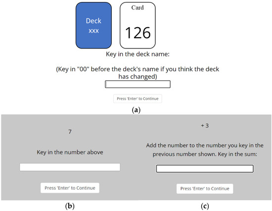
Figure 3.
(a) An example of a trial in the GET. In this trial, a card with the number 126 was shown. The participants must type in the deck name, which is the mean of the cards from a deck. If they think that the deck has changed, they must type ‘00’ before typing the deck name. Example trials in the Summation task shown (b) during the first Summation trial or when the summation resets after incorrect response in the last Summation trial, and (c) when responses from the last Summation trial were correct.
Summation task: The stimulus in the Summation task was a single-digit number with or without a ‘+’ sign before the number, as shown in Figure 3b,c. The number ranged from 0 to 9 and was chosen at random in each trial.
N-back tasks: A 2-back task and a 4-back task were included in the experiment. The stimulus in both 2-back and 4-back tasks was a single-digit number ranging from 0 to 9, selected randomly. The number was presented in the center of a gray border. The color of the gray border could change to red or green based on the participant’s response in each trial.
3.2.2. Procedure
Gaussian Estimation task (GET): In the GET, a numbered card was drawn and displayed to participants in each trial. The participants’ task was to identify the deck name to which the card belonged. Cards from several decks were stacked together without shuffling. Each card displayed only a number, as shown in Figure 3. Participants were informed that the name of a deck corresponds to the mean of all the cards in that deck. For example, if the cards in a deck were 108, 110, 111, 113, and 110, the rounded mean would be 110, and the deck name would be 110. In each trial, a card was drawn from the stacked decks and presented to the participant. They were required to type the number representing the deck name for each trial. If they suspected a deck change, they were to indicate so. Participants might perceive a deck change if there was a noticeable difference in card numbers displayed.
The GET consisted of eight blocks, each comprising 50 trials, for a total of 400 trials. These blocks encompassed eight distinct conditions, detailed in Table 1. As can be seen, different conditions were created for comparing card spread (σ), the number of decks (d), and CLE. The order of blocks was randomized in the experiment. For each block, σ and d were manipulated to reflect variations in perceived noise and environmental volatility. Each block contained a specified number of decks, denoted as d. However, the number of cards per deck within a block was not fixed, preventing participants from accurately estimating when a deck change would occur. Figure 4 illustrates the card numbers displayed across trials within a block, showing variations in σ and d.

Table 1.
The spread of cards, number of decks, and presence of CLE in each block of GET.
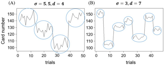
Figure 4.
An example of the card number shown in a given block, with (A) showing greater noise ( and less volatility ( than (B). Blue circles indicate the grouping of cards from the same deck.
Summation task: A summation trial was added to the end of each GET trial within blocks featuring the CLE. In the first summation trial, a randomly chosen number between 0 and 9 was presented, and participants were instructed to key in the displayed number. Starting from the second summation trial, participants were required to remember the cumulative total from the previous summation trial and add it to the current displayed number. If correct numbers were entered, the cumulative sum would be carried forward. Incorrect entries reset the summation process, displaying a new random number for the next summation trial. This task imposed a cognitive load, requiring participants to retain numbers while performing GET trials. In blocks without the CLE, summation trials were replaced by a 1 s break featuring a crosshair in the center of the screen. The task flow of the GET is illustrated in Figure 5.
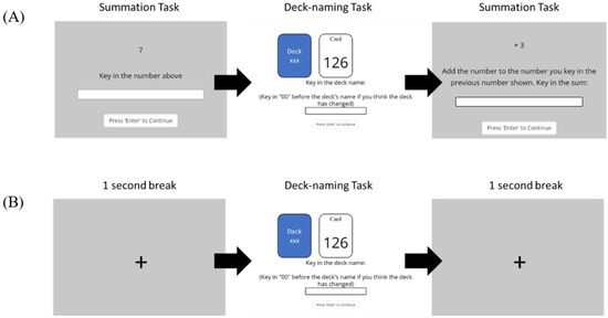
Figure 5.
The task flow of the GET for (A) odd-numbered blocks (blocks 1, 3, 5, and 7), and (B) even-numbered blocks (blocks 2, 4, 6, and 8). The GET trials were presented on a white background while the Summation trials and the crosshair in the 1 s break were presented on a gray background. The blocks were shown in randomized order.
N-back tasks: The 2-back and 4-back tasks were given to participants before the GET. In the 2-back task, participants had to determine whether the number presented in the current trial matched the number displayed two trials ago. The 4-back task was identical except that they needed to determine if the current number matched the number from four trials ago. Both tasks consisted of 60 trials, with 20 match trials where the numbers presented matched the ones shown 2 or 4 trials ago, depending on the task. In each trial, a number was displayed for 1.5 s within a square with a gray border. Participants were required to press the ‘m’ key on the keyboard within 1.5 s if they believed there was a match. If the ‘m’ key was not pressed, the square border remained gray. When the ‘m’ key was pressed, the border turned green on match trials and red on non-match trials.
3.3. Results
3.3.1. Estimating the Reliance on Information in GET
Figure 6A shows the mean number of estimated deck changes across participants for each block. Participants tended to overestimate the number of deck changes when the card distribution had a high spread (σ) or when the actual number of decks in the environment was low. Multiple regression analysis was conducted to examine whether the spread of the card distribution (σ) and the actual number of decks significantly predicted participants’ overestimation of deck changes (estimated number of deck changes—actual number of deck changes). The result of the regression indicated that the two predictors explained 17% of the variance . It was found that the spread of cards significantly predicted the participant’s overestimation in the number of deck changes (), as did the actual number of decks ().
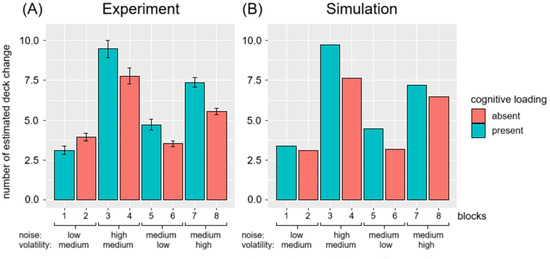
Figure 6.
Mean number of estimated deck changes across (A) participants and (B) simulations for each block in the GET. Block conditions follow the conditions as stated in Table 2 in order. The teal bars are blocks with cognitive loading and the red bars are blocks without cognitive loading. Error bars in the left panel indicate the standard error deviation of the number of estimated deck changes across participants. The black solid line in the left panel is the actual number of deck changes in each block.
Moreover, the overestimation increased significantly under CLE when the card spread was high. The effect was observed in the following: high spread, moderate number of decks (Blocks 3–4: ); moderate spread, low number of decks (Blocks 5–6: ); and moderate spread, high number of decks (Blocks 7–8: (). However, participants detected fewer environmental changes under CLE when the environment had low spread and moderate number of decks (Blocks 1 and 2): ().
Deck name accuracy was calculated by comparing participants’ responses to the calculated deck name for each trial in a specific block. The calculated deck name for each trial was the mean of the card numbers shown since the last estimated deck change. When participants indicated a deck change, the number on the card was used as the calculated deck name for that trial. As trials progressed, the calculated deck name represented the mean of all cards shown after the estimated deck change. Deck name accuracy was determined by the difference between the participant’s response and the calculated deck name for each trial. The mean difference between deck names and the calculated deck means for all eight conditions was small and not statistically significant (, remaining within the range of .
Maximum likelihood was used to fit each participants’ responses in the GET to an equation [25] corresponding to an exponentially weighted moving average, combining the initial values and past observations with a time-decaying weight to estimate the deck’s mean (μt) on a trial-by-trial basis. The decay speed was used to estimate how strongly past outcomes influenced the calculation of μt. Higher indicated greater reliance on past outcomes. Differences in between conditions with and without the CLE indicated variations in reliance on past outcomes, with lower reliance (lower observed under conditions featuring the CLE. An example of μt and participants’ responses to the deck mean is shown in Supplementary Figure S1. τ was estimated separately for each participant and each block of the GET by fitting their responses, and then averaged across participants, as shown in Figure 7. Consistent with the hypothesis, the mean of τ was lower in blocks with cognitive loading compared to blocks without.
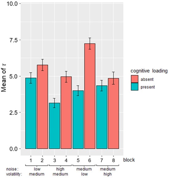
Figure 7.
Mean of across participants for each block in GET. Block conditions follow the conditions as stated in Table 2 in order. The teal bars are blocks with cognitive loading and the red bars are blocks without. Error bars indicate standard error of across participants.
3.3.2. Performance in N-Back Tasks
The performance in both the 2-back and 4-back tasks were calculated as the multiplication of hits and 1-false alarm in detecting the match. Participants, on average, performed more accurately in the 2-back task (M = 0.64, SD = 0.17), with higher hits (M = 0.7, SD = 0.19) and lower false alarms (M = 0.083, SD = 0.048), compared to the 4-back task (M = 0.39, SD = 0.13), with lower hits (M = 0.46, SD = 0.16) and higher false alarms (M = 0.13, SD = 0.082). As shown in Table 2, the accuracy performance in both 2-back and 4-back tasks was correlated with the difference in τ between blocks with the same σ and d but differing in CLE. Table 2 showed a significant positive correlation () for the 2-back accuracy and the difference in τ in Blocks 5 and 6 (moderate spread, low number of decks), as well as a trending negative correlation () for the 4-back accuracy and the difference in τ in Blocks 3 and 4 (high spread, moderate number of decks). The relationship of the n-back accuracy and the difference in in Blocks 3, 4 and Blocks 5, 6 (moderate spread, low number of decks) are shown in Supplementary Figure S2. With the results, it was shown that the cognitive loading impacts correlated with the performance in the n-back task when the card spread was high and when volatility in the environment was low.
Table 2.
The correlation of the difference in τ in the paired blocks for CLE (blocks with the same card spread and volatility but different cognitive loading) and the n-back accuracy in each participant.
In the blocks with significant or trending correlations, the analysis explored the relationship between hits, false alarms, and τ for Blocks 3–6. Table 3 showed that participants with a higher τ in Block 3 had higher hits in the 4-back task and lower false alarms in the 2-back task. Similarly, participants with a greater τ in Block 5 had lower false alarms in the 2-back task. The stronger correlation of τ in Block 5 and hits in the 4-back task may be attributed to the increased difficulty in detecting deck changes when card spread was high in Block 5 and the elevated WM demand in the 4-back task.
Table 3.
The correlation in τ in blocks 3–6 and the n-back accuracy in each participant.
3.3.3. Summary of Behavioral Results
In short, participants tended to overestimate the number of deck changes, particularly under high noise (spread) conditions. Their overestimation was amplified under cognitive load, indicating impaired uncertainty estimation when WM resources were taxed. Despite this, participants demonstrated the ability to estimate deck mean, as evidenced by small deviations between the calculated deck mean and the reported label. Under dual-task conditions with CLE, reliance on past outcomes decreased, particularly in blocks with high spread or low volatility, where greater WM engagement was required. The magnitude of this reliance difference correlated with WM capacity: higher 2-back performance predicted greater reliance on past outcomes between Blocks 5 and 6, indicating a larger reliance on past outcomes when participants had higher WM capacity. Conversely, lower 4-back performance showed a trending negative correlation with outcome reliance between Blocks 3 and 4, showing smaller reliance when participants had lower WM capacity.
3.4. Simulation with the New Model
The GET was simulated with the new model. In each trial, the model input was a number generated from the Gaussian distribution that followed N (deck’s mean, ). The statistics of the Gaussian distribution for the numbers followed the structure from the experiment as shown in Table 3. The P (n + 1) generated at the end of each trial was used as the response for the deck’s name, while C from Equation (5) was used as the response for the perceived change in environment.
The parameter values used for the simulation were estimated using grid search (Appendix A Table A2). To simulate the CLE, the value of I from Equation (6) was lowered (I = 0.88) under conditions where CLE was present compared to the condition where CLE was absent (I = 0.93). A lower I reduced outcome weights to a greater extent as the number of WM-stored outcomes increased. When outcome weights were reduced below the threshold, the corresponding outcome that was previously stored in WM was gated-out of WM.
Simulation Results from the Model
The number of estimated deck changes for 200 simulations is shown in Figure 6B. The number of estimated deck changes was simulated with a RMSE of 0.487 and r2 = 0.99. Figure 6B shows that a lower I (with CLE) in the model causes overestimation of deck changes compared to the conditions with higher I (without CLE). The average expected uncertainty computed for the blocks with CLE was less than that observed in the blocks without CLE. This difference is illustrated in Table 4, where positive values indicate a greater average Ue in blocks without CLE compared to corresponding blocks with CLE.
Table 4.
Difference in average Ue between blocks with and without CLE.
Furthermore, Figure 8a shows the grand mean number of outcomes retained in WM in the trials before a change was detected within each block. The mean number of outcomes stored in WM was obtained by averaging the stored for the trials before a change was detected in a block of a simulation. The grand mean number of outcomes stored in WM across trials was obtained by averaging the mean across all simulations. This represents the number of WM-stored outcomes for the trial. The WM-stored outcomes were higher in blocks without CLE compared to the blocks with CLE.
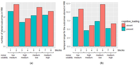
Figure 8.
(a) The grand mean number of stored outcomes in WM across trials in each block. Error bars indicate the standard error of the mean number of outcomes stored in WM across trials. (b) The grand mean of temporal range for the outcomes stored in WM across trials in each block. Block conditions follow the conditions as stated in Table 3 in order. The teal bars are blocks with cognitive loading and the red bars are blocks without cognitive loading.
In addition, the grand mean of the temporal range of the stored outcomes in WM for each block is shown in Figure 8b. The temporal range of the stored items in WM was obtained by subtracting the time occurrence of the outcome that stayed the longest in WM from the trial before a change was detected. The grand mean of the temporal range for the outcomes in WM was higher in blocks without CLE compared to the blocks with CLE.
In short, more outcomes were stored in WM in blocks without CLE compared to the corresponding blocks with CLE. Similarly, past outcomes stayed longer in WM in blocks without CLE compared to the corresponding blocks with CLE. This indicated that more outcomes from the past could be recalled and utilized to form uncertainty estimation for outcome estimation.
3.5. Discussion
3.5.1. Misestimation of Expected Uncertainty Due to Smaller Sample Size in WM
The results showed that participants relied less on past outcomes in blocks with CLE because part of their cognitive resources were engaged in the summation task. The model simulated this decrease by increasing lateral inhibition in WM, thus reducing the weights of past outcomes when more outcomes were stored. This higher rate of weight reduction in CLE blocks allowed the model to match participants’ perceived number of deck changes.
With increased card spread, participants generally perceived more deck changes in CLE blocks compared to non-CLE blocks. The model indicated that CLE, represented as reduced I, led to a smaller outcome sample size in WM. While this limited sample size was sufficient for estimating the mean, it was inadequate for estimating variance, potentially misrepresenting the deck’s distribution and lowering expected uncertainty. Outcomes exceeding this reduced uncertainty triggered a gating-out mechanism in WM, leading to deck change detection. Thus, greater WM interference with WM-stored outcomes lowered the estimated deck noise (card spread in the deck) and contributed to overestimation of the number of deck changes.
While the model successfully captured the general influence of WM capacity on perceived deck changes, it failed to replicate the observed distinction between Blocks 1 and 2. Behavioral results showed that participants detected more deck changes in Block 2 than in Block 1, indicating a reversal effect of WM interference on the perceived number of deck changes when the card spread was relatively low. In the model, a sufficiently high H amplified the estimation of expected uncertainty when fewer outcomes were stored in WM, an effect more pronounced under heightened WM interference due to reduced WM size.
Despite attempts to model this reversal effect, the model could only narrow the gap in perceived deck changes between the two blocks by adjusting WM interference based solely on the presence of CLE. However, it should have underestimated expected uncertainty in a low-noise environment under greater WM interference. The model’s failure to achieve this may stem from the similarity in the number of outcomes stored in WM across trials in both blocks. In a low-noise environment, drawing a card within the same deck resulted in low surprise. Consequently, expected uncertainty in Blocks 1 and 2 differed minimally, leading to comparable perceived deck changes across these blocks.
3.5.2. Relating Participants’ Reliance on Past Outcomes in GET to WM Capacity
Furthermore, the experiment examined the relationship between reliance on past outcomes in GET and WM capacity, as measured by the N-back tasks. Significant correlations emerged only under high card spread or low deck change conditions. Under low-demand GET conditions (low volatility and moderate spread), participants who relied more on past outcomes under CLE but less without CLE showed lower 2-back accuracy, indicating reduced WM capacity. In contrast, under high-demand GET conditions (moderate volatility and high spread), participants with inconsistent reliance (lower under CLE, higher without) also performed worse than those with stable reliance with and without CLE. In the 2-back task, accuracy differences were primarily due to variation in false alarms, with hits showing little variation. In contrast, the increased task demand of the 4-back task made successful hits more challenging, suggesting that performance differences were mainly driven by hit accuracy.
Hits in N-back tasks likely reflect the ability to retain relevant information in WM, while false alarms suggest difficulty in discarding irrelevant information. In the 4-back task, participants who relied less on memory under demanding GET conditions with CLE performed poorly, emphasizing the need to retain relevant data and minimize loss for successful hits. WM capacity is not fixed but instead influenced by factors like familiarity and the nature of the information [47]; the lack of conceptual meaning in the taxing 4-back task may have hindered active storage of information. Retaining larger amounts of data may require greater active WM storage [48,49], with individual differences becoming more evident in noisy environments.
In the 2-back task, the ability to discard irrelevant information, a key component of the gating-out mechanism in WM [50], likely helped reduce false alarms. Participants who over-relied on past memories under low-demand GET conditions with CLE likely retained outdated information when it was no longer relevant. This tendency was especially noticeable in environments with minimal changes and low-to-moderate card spread, which produced fewer unexpected outcomes. These findings suggest that information updating or inhibition play a significant role in task performance and should be explored further in relation to executive functioning.
3.5.3. Limitation
A limitation of the experiment was the model’s assumption of a uniform WM interference effect under CLE conditions. The impact of memorized items from summation trials on outcome storage likely varied, especially when participants failed to remember summation numbers, reducing CLE’s influence on perceived deck changes. Additionally, the model did not account for interference from stimulus similarity [51,52]. Although GET outcomes used three-digit numbers and summation trials used single-digit numbers, overlap could still occur. The model assumed perfect memory for stored outcome, with interference only affecting the retention weight, potentially misinterpreting actual memory dynamics.
Another limitation was data quality. Many participant responses were random or unrelated, leading to substantial data exclusion. The issue stemmed from limited control over inputs in an online setup and potential task disengagement due to task complexity or monotony. Future replications in a controlled lab environment could mitigate these data quality concerns.
4. Ability to Differentiate Variance in Outcome
This section extended previous findings on environmental change detection under constant noise by examining how changes are detected when outcomes transition between noisy and consistent states. The experiment explored how exposure to observations affects detection of different types of distributional changes: shift in mean, variance decrease, and variance increase while maintaining the mean. Findings showed that limited WM capacity and insufficient exposure to outcomes elevated expected uncertainty, impairing the detection of these transitions. Greater outcome exposure improves change detection by enabling better tracking of expected uncertainty, suggesting a potential mechanism for adapting to a changing environment under constrained memory resources.
4.1. Participants
The sample sizes from power analysis with GPower 3.1 [53] was 66 (lenient effect size for one-way ANOVA comparing the accuracy between the three blocks of trials, where = 0.05, power = 0.95, and effect size = 0.5). A total of 148 participants were recruited from the Purdue University undergraduate population. Each participant was given credit for participation as partial fulfillment of a course requirement. Research protocols were approved by Purdue University’s Institutional Review Board (IRB No. IRB-2023-298) and were conducted in full compliance with institutional and ethical guidelines for research involving human participants, including the Declaration of Helsinki of 1975.
4.2. Task in the EXPERiment
4.2.1. Materials
The tasks were displayed on a 21-inch monitor with 1920 × 1080 resolution. The experiment was controlled by in-house programs written using PsychoPy v3 [54]. The experiment involved a card game where participants determined whether two piles of cards originated from the same deck. The primary aim was to assess participants’ ability to distinguish between decks that differed only in card spread versus those that differed only in the mean of the cards under varying levels of card exposure. The experiment featured three conditions: Conditions L, M, and H. Under each condition, there was an equal chance that the two piles came from the same or different decks. For cards from different decks, Condition M involved variations in mean with constant variances. In contrast, Conditions H and L examined variations in variance while keeping the mean constant. Specifically, under Condition H, the variance in the first deck was greater than that of the second, whereas under Condition L, the reverse was true.
For all conditions, the card numbers presented to participants (detailed in Supplementary Table S1) were preselected prior to the experiment. These numbers were chosen to represent the full range of each deck accurately, even when only a limited number of cards was shown (as explained in the subsequent subsection). Each pile’s card numbers were drawn from a Gaussian distribution with a predefined mean and variance. Participants indicated their responses by pressing either the ‘Y’ button (mapped to the ‘s’ key) or the ‘N’ button (mapped to the ‘k’ key).
For trials involving cards drawn from different decks, the variance and mean of the decks were selected to position the Kullback–Leibler (KL) divergence of Condition M between those of Conditions H and L. Table 5 presents the KL divergences between the first and second decks shown to participants for each trial and condition. The objective was to ensure a balanced difficulty level in distinguishing between decks in Condition M, making it neither too easy nor too difficult compared to Conditions H and L.
Table 5.
The KL divergence of the two different decks presented to the participant in each trial of a given condition.
Under both Conditions H and L, the variance difference and mean of the two decks were identical. The key distinction was the order in which the decks were presented: under Condition H, the deck with higher variance was shown first, while under Condition L, it was shown second. This suggested that distinguishing between decks became easier with increased variability in outcomes, as opposed to when outcomes became more consistent. The card numbers within each deck were chosen to align the variance and mean of the card numbers with the distributional characteristics of the deck.
4.2.2. Procedure
Participants were informed about multiple decks of cards, from which n cards were drawn and placed on the left and right sides. Cards could be drawn from the same deck or different decks. Each trial began with one pile of cards being shown sequentially until all cards were displayed. The process then moved to the other pile. The task flow for each trial is illustrated in Figure 9b. After all cards were shown, participants were asked if the two piles were from the same deck. The trial ended once the participant made a response, and the next trial began.
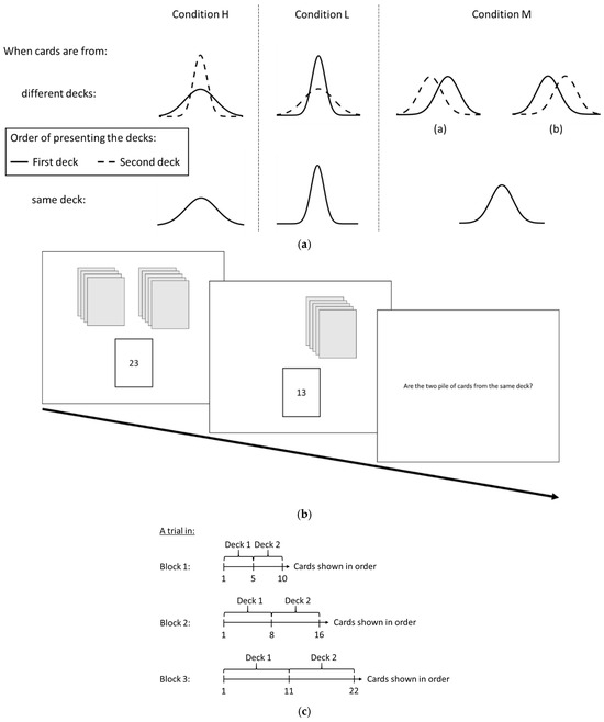
Figure 9.
(a) The distribution of the deck to which the cards belong for each condition. Solid lines indicate the deck that the cards were first drawn and shown. Dashed lines indicate the deck that cards were drawn and shown after all cards from the first deck were all shown. (b) Task flow in each trial of the experiment. (c) The number of cards presented to the participants from the two decks in a trial for different blocks. Cards from the second deck were only presented after all cards from the first deck were shown. The first deck could be positioned on either the left or right side of the screen, with the second deck on the opposite side. The order of presenting the cards, either from left to right or right to left, was counterbalanced, ensuring an equal chance of starting with either deck.
The experiment was designed to investigate how the detection of deck dissimilarity increases as more cards are presented in each trial. It consisted of three blocks, each containing 32 trials, with three conditions: 8 trials of Condition L, 8 trials of Condition H, and 16 trials of Condition M. The number of cards shown varied across blocks, as illustrated in Figure 9c. In Block 1, participants saw 10 cards (5 per pile), in Block 2, 16 cards (8 per pile), and in Block 3, 22 cards (11 per pile). Both trials within each block and blocks themselves were presented in a randomized order. At the end of each trial, participants indicated whether the two decks were the same or different by pressing ‘Y’ or ‘N’ on the keyboard. Their binary responses were recorded for accuracy in detecting changes in deck distributions.
4.3. Experimental Results
The accuracy of determining deck similarity is shown in Figure 10a, while d′ [55,56], a measure of sensitivity to changes, is displayed in Figure 11a. The analysis only included data collected from participants whose accuracy surpassed chance levels under Condition M, as poor performance may indicate difficulty in distinguishing distribution differences or inattentiveness. Following the exclusion criteria, 103 out of the initial 48 participants were included in the study for analysis.
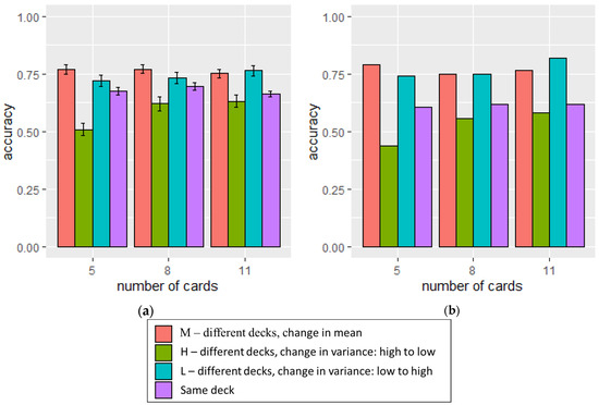
Figure 10.
The accuracy of determining whether the decks were the same or different was assessed under each condition, with the number of cards presented varying for (a) the participants in the experiment and (b) in the simulation. The error bars in the left panel indicate standard error of the accuracy across participants.
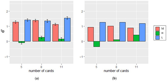
Figure 11.
The d′ under each condition with the number of cards presented varying for (a) the participants in the experiment and (b) in the simulation. The error bars in the left panel indicate standard error of d′ across participants.
Participants exhibited the highest performances under Condition L (M = 0.79, SD = 0.18), followed by Condition M (M = 0.73, SD = 0.14), and finally Condition H (M = 0.52, SD = 0.20). A repeated measures ANOVA was conducted to examine the effect of card distribution (Conditions M, L, or H) and number of cards on participant’s accuracy. A significant main effect of type of card distribution was observed, with F (2, 586.28) = 129.487, p < 0.001. In addition, a significant interaction effect between the number of cards and the type of card distribution was also found, with F (4, 408) = 4.742, p < 0.001. However, the main effect of the number of cards presented to the participants in a given trial was not statistically significant, with F (2, 605.62) = 2.357, p = 0.096. The results showed that participants performed differently across various card distributions. Additionally, discerning dissimilarity was easier when the cards’ spread increased, compared to when it decreased.
Separate ANOVA analyses were conducted to examine the effect of the number of cards on accuracy under each condition. A significant effect was observed under Condition H, with F (2, 306) = 3.76, p = 0.024. However, the effect was not significant under Conditions L (F (2, 306) = 1.497, p = 0.225) and M (F (2, 306) = 2.186, p = 0.114). This indicated that participants’ performance varied depending on the number of cards presented to them when the spread of the cards decreased.
Paired t-tests were conducted to examine whether participants performed better when more cards were presented under Condition H. Participants demonstrated significantly higher performance when presented with 11 cards compared to the situation with 5 cards, with t (102) = 3.076, p = 0.001. Similarly, the performance was significantly better when presented with 8 cards compared to the situation with 5 cards, with t (102) = 2.520, p = 0.007. However, no significant difference was observed when they were presented with 11 cards and 8 cards, with t (102) = −0.729, p = 0.766. The results indicated a possible optimal level of outcome exposure for maximizing accuracy, beyond which additional exposure provided limited benefits to performance.
4.4. Simulation with the Full Model
The three blocks in the experiment were simulated with different numbers of cards (10 for Block 1, 16 for Block 2, and 22 for Block 3). The model takes in the , which were card numbers from each deck that were presented to participants in the experiment. The model was presented with an identical pair of card sets as those shown to the participants. However, the card numbers in each deck were randomized in each simulation. Card numbers from the second deck were presented to the model after all card numbers in the first deck were presented.
In the model, deck change only occurred when the outcomes came from the second deck. A deck change was detected when urge from Equation (8) exceeded the set threshold. This change happened when either the mean of relevant outcomes (MeanO) deviated significantly from the predicted outcome (P) with respect to expected uncertainty (Ue), or when the variance in recent outcomes stored in WM either steadily decreased or increased compared to the variance in older outcomes, using the function for CΔvar in Equation (9). The accuracy of detecting deck changes for 250 simulations with RMSE of 0.04937 and r2 = 0.98 was shown in Figure 10b, while d′ with RMSE of 0.2662 and r2 = 0.98 was shown in Figure 11b.
To fit the data, the only change to the parameters in the model was , which is the rate of shifting from the bias term ( to variance in relevant outcomes ( in the expected uncertainty (. The value of was the lowest under Condition H ( = 0.75), followed by Condition L ( = 1), and finally Condition M = 5). A lower value of indicated a lower reliance on the bias term to compute expected uncertainty as the number of outcomes stored in WM increased. Under Condition H, expected uncertainty was closer to the variance in relevant outcomes even when the number of outputs stored in WM was low. The parameter values for the remaining free parameters that remained the same throughout the simulation are listed in Table 6.
Table 6.
Free parameters in the simulation that stayed constant across all simulations (different from Experiment 1).
4.5. Testing Model Components
In the experiment, no manipulation of the CLE on WM was performed to assess the importance of WM constraints in environmental change detection. To understand the influence of WM constraints on environmental change detection, a comparison was made between the simulation that considered each outcome and the participants’ behavioral results. Additionally, considering the hypothesis that a separate mechanism with variance comparison was required for detecting changes in card distribution, the study further examined conditions where the variance comparison mechanism was omitted to assess the extent to which the model could simulate the same effect without it.
4.5.1. Perfect Memory
The significance of the WM gating mechanism was assessed by simulating a scenario of perfect memory. This was achieved by keeping all outcomes presented into WM without gating them out through WM interference. The accuracy in detecting deck changes (RMSE = 0.1862, r2 = 0.38) was shown in Figure 12A, while the d′ (RMSE = 0.4912, r2 = 0.86) was shown in Figure 12B. With this simulation, the accuracy in detecting a deck change when cards were from different decks under Condition H changed drastically. Accuracy was lower than the participant’s result when only five cards were presented, and it increased significantly when eleven cards were presented. The accuracy when cards are from the same deck for all three conditions combined was generally higher compared to the participant’s result. The greatest difference in d′ values compared to the participant’s result was observed when eleven cards were presented under Condition H, which exceeded the d′ obtained from the experiment by a substantial margin.
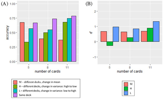
Figure 12.
Perfect memory scenario: (A) The accuracy of determining whether the decks were the same or different was assessed under each condition, with the number of cards presented varying in the simulation. (B) The d′ under each condition, with the number of cards presented varying in the simulation.
4.5.2. Comparing Outcome Variance Across Time
In addition, the simulation was executed without the inclusion of outcome variance comparison over time. This step aimed to assess the effect of detecting deck changes under Condition H when only the variance in the cards changes from high to low. The accuracy in detecting deck changes (RMSE = 0.3180, r2 = 0.58) was shown in Figure 13A, while the d′ (RMSE = 0.52, r2 = 0.63) was shown in Figure 13B. Under Condition H, accuracy when cards were from different decks was significantly lower compared to participants’ results. This lower accuracy indicated the challenge of detecting a deck change using only the surprise function. Moreover, the negative d′ value under Condition H was observed. Removing the outcome variance comparison also affected accuracy under other conditions, notably in Condition M, where the ability to detect deck changes decreased drastically when exposed to more outcomes.
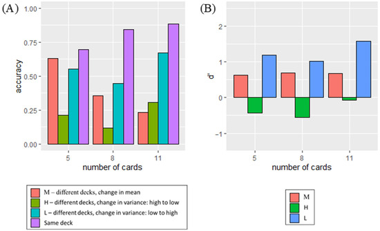
Figure 13.
Excluding outcome variance comparison over time: (A) The accuracy of determining whether the decks were the same or different was assessed under each condition, with the number of cards presented varying in the simulation. (B) The d′ under each condition, with the number of cards presented varying in the simulation.
4.6. Discussion
The experiment assessed participants’ ability to detect changes in outcome distributions when either the variance (noise) or the mean shifted, and whether detection performance varied with the amount of exposure to outcomes. Specifically, the study compared detection accuracy across conditions where outcome variance increased, decreased, or remained constant with a mean shift.
Results showed that the order of outcome presentation (e.g., high-to-low vs. low-to-high card spread) influenced participant’s ability to discern distinctions between distributions. Performance mirrored KL divergence across conditions: detection was highest with increased variance, followed by mean shifts, and lowest with decreased variance. As outcome exposure increased, participants’ ability to detect deck changes remained stable with mean shifts or increased variance and improved significantly when variance decreased, though increased exposure did not fully offset the reduced detectability under low-variance conditions. Future work should examine how participants determine whether they have observed enough data to form reliable estimates of environmental change.
4.6.1. Simulating Change Detection in Different Outcome Distribution
The model evaluated change detection across conditions where outcome uncertainty varied. Detection occurred when outcomes diverged from the WM-stored mean, either gradually through accumulated shifts or abruptly via WM rests triggered by surprising events, both relying on mean shifts. However, under Condition H, outcomes remained within the prior range, preventing significant mean shifts or WM clearance, and simulations (without variance comparisons) showed reduced detection accuracy. This suggests that tracking outcome mean alone is insufficient to explain experimental results, indicating the need for additional mechanisms.
Simulation adjustments showed that reliance on initial expected uncertainty estimates influenced detection: Condition M relied most on initial estimates, followed by L and H. Under Condition M, detection depended on mean shifts; under Condition L, both mean and variance contributed; and under Condition H, detection primarily relied on variance changes. This highlights the increasing importance of outcome variance tracking for detecting distributional changes from Conditions M to H.
4.6.2. Simulating Change Detection with Greater Outcome Exposure
In the actual simulation of behavioral results, increased exposure minimally improved deck change detection accuracy under Conditions M and L compared to Condition H. This suggests that exposure influenced mean shift detection less than variance comparisons, especially under WM constraints where stored information changed gradually. In contrast, perfect memory simulations showed greater exposure reduced sensitivity to mean shifts, as adding new outcomes had little effect on the mean estimate when many outcomes were already stored, decreasing change detection accuracy.
Conversely, for variance comparisons, the model showed improved change detection with more exposure, likely due to clear separation between older and newer outcome sets. Yet, this benefit may plateau, indicating a potential saturation point beyond which additional exposure does not further enhance variance detection. Future research should examine this potential limitation.
4.6.3. Limitations
In this experiment, one limitation was the limited variability in the changes in variance and mean in the card distribution. The differences in variance and mean were carefully chosen to ensure that the task of distinguishing two distributions did not become too easy or too difficult. Varying the variance and mean differences would alter the ability to differentiate between the two distributions, which was intentionally controlled in the study. However, this control could potentially lead to predictability in the changes where participants anticipate detecting a change in predictability rather than truly detecting a change in the deck, which might serve different goals. Another limitation of the study would be the lack of a mechanism for guessing in the model. In the model, detecting a change was contingent on the presence of sufficient evidence indicating a change. However, the model did not consider the possibility of confidence in decision-making when evidence was close to reaching a clear threshold. Introducing a noise factor could have been a useful way to address this issue.
5. General Discussion
To investigate outcome estimation in human learning, we proposed a model that emphasizes the role of WM constraints [57,58] in forming uncertainty estimates to detect environmental dynamics. The model uses lateral inhibition to represent interference that limits WM capacity, particularly affecting the gating mechanism that retains relevant information and removes those that became irrelevant [50], guided by surprise signals [59,60,61] and a top-down perception of environmental relevance. The study addressed a gap in prior research that often imposed memory limits by providing a mechanistic account of WM capacity effects in uncertainty estimation through lateral inhibition as stored information increased.
The model was tested through experiments investigating how limited WM capacity affects misestimation of perceived volatility and noise, and how participants detect environmental changes under varying noise levels and outcome exposure. Experiment 1 showed that cognitive load reduced WM storage, lowering expected uncertainty and increasing misinterpretation of unexpected outcome as environmental changes. Experiment 2 found that participants detected noise increment better than reduction, with greater exposure improving the latter. These results highlight distinct mechanisms facilitating uncertainty estimation under constrained WM resources.
5.1. Do More Outcomes Mean Better Accuracy? Balancing Evidence and Accuracy
In daily life, we infer hidden aspects of the world from noisy and constantly changing observations. Research work from Tavoni et al. [25] revealed that while complex and probabilistic methods like Bayesian inference offer high accuracy, they demand extensive memory and processing, whereas simpler heuristics are less cognitively demanding but offer less precision. Our findings highlight this tradeoff, showing increased outcome exposure often yields only minimal gains in accuracy, aligning with bounded rationality [62,63], which posits that individuals make decisions within cognitive and informational constraints, settling for satisfactory rather than optimal solutions.
Intriguingly, the inclusion of more outcomes led to improved deck change detection in Experiment 1, but increased outcome exposure did not necessarily translate into improved accuracy; instead, it resulted in decreased performance when simulated with perfect memory. This discrepancy reflects differences in the task structure’s indication of deck change and demonstrates how WM limitations, modeled via lateral inhibition and interference, constrain benefits from additional exposure. The lack of increment or advancement in performance could potentially characterize the stopping rule in adaptive exploration or a saturation point in sampling due to WM constraints. This raises future questions on how cognitive resource loading influences exploration of stopping rules, particularly when adaptive sampling may be influenced by outcome uncertainty [64], and how such mechanisms relate to boredom-driven exploration that eventually drives individuals to explore other possible options [65].
5.2. Misestimating Environmental Statistics
The study examined whether outcome estimations rely on uncertainty assessments under various environmental conditions. Tavoni et al. [25] suggested that memory is less critical for outcome estimation when noise is low, regardless of volatility, a finding supported by our simulations showing that WM size had little influence under a stable and consistent environment, where early uncertainty guesses sufficed. However, when environmental noise increased, more outcomes were gated into WM based on their unexpectedness, reducing reliance on past outcomes. This aligns with Tavoni et al. [25], indicating that in noisier, more volatile environments within manageable bounds, retaining and integrating more outcomes becomes advantageous. However, adapting to such uncertainty may require extended learning [66] and neural adaptations to unexpected outcomes [14], which enhance meta-learning and attention [6,67,68].
Misestimating environmental noise, conversely, stemmed from inaccuracies in expected uncertainty computed from WM-stored outcomes, particularly when initial guesses deviated from true-noise levels. Simulations showed this effect was amplified under cognitive load due to WM constraints. Greater storage of outcomes in WM displaced expected uncertainty away from initial guesses, improving environmental noise estimation accuracy. These results highlight the interplay between WM capacity, initial beliefs, and environmental noise in shaping uncertainty estimations.
5.3. Information Processing in Outcome Estimation: Balancing Prioritization of Recent and Distant Past Information
The current study raised questions on whether individuals prioritize recent outcomes or rely on earlier information for outcome estimations, especially when frequent updates of environment representations were deemed unnecessary. In Experiment 1, without cognitive load, participants showed high reliance on distant past outcomes, especially in stable environments with low noise and volatility, suggesting fewer new inputs are integrated unless surprising, resulting in lower cognitive effort [69,70]. This indicates that the typical recency effect [71] was outweighed by the primacy effect [72], where early experiences were weighted more heavily, aligning with strategic prioritization frameworks [66]. Such a strategy may hinder detection of subtle environmental changes, as continuous updates can smooth over gradual shifts. Understanding when to rely on prior versus new information is thus critical for detecting true changes, discerning causal relationships, and determining which cues are most reliable for guiding future decisions.
6. Conclusions
This study highlights the critical role of WM constraints in shaping uncertainty estimation and environmental change detections. By integrating a WM gating mechanism with lateral inhibition into a computational model, the model accounted for systematic misestimations under cognitive load and limited outcome exposure.
Quantitatively, the model demonstrated that cognitive loading impaired deck change estimations, yielding an RMSE of 0.487 with an R2 of 0.99. Additionally, the model estimated deck changes performance involving environmental noise and mean shifts across varying levels of outcome exposure with an RMSE of 0.049 and R2 of 0.98. Its sensitivity to change detection was also high, with an RMSE of 0.26 and R2 od 0.98.
The novel contributions from the study include the following:
- A novel mechanism for estimation of uncertainty incorporating WM gating modulated by outcome interference.
- Empirical validation linking EM capacity, cognitive load, and uncertainty misestimation.
- Insights into the balance between evidence accumulation and information saturation with limited cognitive resources.
Overall, these findings advance the understanding of decision-making under cognitive constraints and provide a foundation for models incorporating memory limitations in reinforcement learning.
6.1. Limitations
The current model assumes that all past experiences relevant to uncertainty estimation are stored and processed within WM, but this overlooks the role of long-term memory, which retains information over extended periods and interacts with WM during outcome estimation over time [73,74]. While long-term memory is not explicitly modeled, its effect may appear in the model’s initial expected uncertainty guesses or in shaping outcome estimates. Future models could benefit from incorporating long-term memory mechanisms in improving the model’s realism by adding stable, high-capacity memory dynamics to uncertainty estimation. Additionally, the model embeds volatility within WM gating to modulate outcome retention, indirectly affecting mean and variance estimates over time. However, it does not model volatility directly as a learning rate modulator, as used in reinforcement learning approaches [40,75], limiting its explanatory scope.
6.2. Future Directions
The study found that under low uncertainty, increased outcome exposure only marginally improved estimation accuracy, suggesting diminishing returns. Future research could examine whether allowing participants to decide when to stop gathering information, rather than using fixed sampling, reveals strategic adaptation under WM constraints. This approach assesses whether decision stopping points reflect diminishing changes in outcome estimation under WM constraints. With our results suggesting that when environmental noise decreases and increased exposure improves performance, participants may delay stopping to gather more informative observations, highlighting implications for an exploration–exploitation dilemma [76,77,78]. While the stopping strategy in exploration may be akin to the concept of adaptation to satisfy [62] and not to optimize, past research [79] showed optimal stopping delays under higher uncertainty. This aligns with directed exploration where participants continue exploring until expected informational gain no longer justifies further search, transitioning to exploitation and rational decision-making [80].
Additionally, Crossley et al. [81] showed that procedural learning resists unlearning under low feedback contingency, but cognitive load can facilitate unlearning, implicating executive functions in this gating process [82]. This raises questions about how WM constraints and uncertainty misestimation might alter perceived feedback contingency under cognitive load and thereby influencing other learning systems in the brain, such as the procedural learning system.
Future work could investigate neurobiological substrates such as the anterior cingulate cortex (ACC), known for monitoring prediction errors or conflicts in cognitive control [83]. Lenartonicz et al. [84] found ACC connectivity differentially related to memory- versus attention-driven performance in WM tasks. Given the close connection between WM capacity and the ACC, this suggests a possible role for WM capacity in shaping choice history, error prediction, and uncertainty estimation.
Furthermore, as the current WM-based uncertainty model examines how memory constraints shape belief updating and outcome estimations, future work could integrate pairwise comparison methods to assess subjective evaluations under uncertainty, particularly when direct estimation is challenging. For instance, participants could judge which of the two outcome sets has a higher mean or greater variability, producing binary preference data. Using pairwise comparisons [85,86], perceptual scales can then be derived from these binary judgments and compared to the model-predicted uncertainty estimates testing whether WM gating mechanisms predict such pairwise-derived weights and further supporting the role of WM in structuring judgements under uncertainty.
Lastly, although this study provides some within-model comparison of WM-based functionality, comparison with other existing models could further clarify the advantages of WM gating in capturing belief updating dynamics relative to alternative memory and decision-making models. Such comparisons could include evaluating our WM-based gating approach against models such as HER [28,29], which emphasizes hierarchical error representations in a biological substrate, and RLWM [22], which integrates reinforcement learning with WM forgetting at a more abstract level. These comparisons would allow for examining how different mechanisms prioritize, weigh, and integrate multiple outcomes under uncertainty.
Supplementary Materials
The following supporting information can be downloaded at: https://www.mdpi.com/article/10.3390/math13152431/s1, Figure S1: Two examples of deck mean: (A) participant’s response (green line) and (B) deck mean from Equation (14)’s output (red line); Figure S2: Relationship of n-back accuracy and the diffrence in in (A) blocks 5 and 6 and (B) blocks 3 and 4. Difference in is calculated as in block 6 − in block 5, and in block 4 − in block 3; Table S1: Card numbers that were shown to participants in Experiment 2.
Author Contributions
Conceptualization, L.X.L. and S.H.; Methodology, L.X.L.; Formal analysis, L.X.L.; Data curation, L.X.L.; Writing—original draft, L.X.L.; Writing—review & editing, R.A. and S.H.; Supervision, R.A. and S.H. All authors have read and agreed to the published version of the manuscript.
Funding
This work was partially funded by the RIKEN Center for Brain Science (CBS)–Toyota Collaboration Center (BTCC) (Grant No. LP3009219), which funded R.A. and the experiments conducted in his laboratory.
Data Availability Statement
The raw data supporting the conclusions of this article will be made available by the authors on request.
Acknowledgments
This work was part of the first author’s doctoral dissertation.
Conflicts of Interest
The authors declare no conflict of interest.
Appendix A
Table A1.
Free parameters in the model.
Table A1.
Free parameters in the model.
| Free Parameters | Represents | Equations |
|---|---|---|
| Regularization for division of zero | (1), (6) | |
| Expected uncertainty coverage | (1) | |
| Base incremental gain used in the logistic function | (3), (6) | |
| Gain associated with the volatility effect | (3) | |
| Shift in the logistic function | (4) | |
| Impact of urge on | (6) | |
| Decay for the reliance on in | (7) | |
| Influence of the accumulated changes in variance | (8) | |
| Scaling factor for variance comparison threshold | (9) | |
| Threshold for WM weights | (6), (7) | |
| Free parameter for the volatility effect | (3), (6) | |
| Initial estimate for | (7) | |
| I | WM interference | (6) |
Table A2.
Free parameters in the simulation that stayed constant for all simulations.
Table A2.
Free parameters in the simulation that stayed constant for all simulations.
| Free Parameters | Parameter Value |
|---|---|
| 0.001 | |
| 9 | |
| 8 | |
| 8 | |
| 3.5 | |
| 0.95 | |
| 3 | |
| 0.7 | |
| 0.08 | |
| 0.9 | |
| 0.85 | |
| 12 |
References
- Bland, A.R.; Schaefer, A. Different varieties of uncertainty in human decision-making. Front. Neurosci. 2012, 6, 85. [Google Scholar] [CrossRef]
- Sutton, R.S.; Barto, A.G. Reinforcement Learning: An Introduction; Cambridge University Press: Cambridge, UK, 1998. [Google Scholar]
- Seymour, B.; Daw, N.; Dayan, P.; Singer, T.; Dolan, R. Differential encoding of losses and gains in the human striatum. J. Neurosci. 2007, 27, 4826–4831. [Google Scholar] [CrossRef]
- Wittmann, M.K.; Kolling, N.; Akaishi, R.; Chau, B.K.; Brown, J.W.; Nelissen, N.; Rushworth, M.F. Predictive decision making driven by multiple time-linked reward representations in the anterior cingulate cortex. Nat. Commun. 2016, 7, 12327. [Google Scholar] [CrossRef] [PubMed]
- Tobler, P.N.; Weber, E.U. Valuation for Risky and Uncertain Choices. In Neuroeconomics: Decision Making and the Brain; Academic Press: Amsterdam, The Netherlands; Boston, MA, USA, 2014; pp. 149–172. [Google Scholar] [CrossRef]
- Monosov, I.E. How outcome uncertainty mediates attention, learning, and decision-making. Trends Neurosci. 2020, 43, 795–809. [Google Scholar] [CrossRef] [PubMed]
- Yu, A.J.; Dayan, P. Uncertainty, Neuromodulation, and Attention. Neuron 2005, 46, 681–692. [Google Scholar] [CrossRef] [PubMed]
- Soltani, A.; Izquierdo, A. Adaptive learning under expected and unexpected uncertainty. Nat. Rev. Neurosci. 2019, 20, 635–644. [Google Scholar] [CrossRef]
- Inglis, J.B.; Valentin, V.V.; Ashby, F.G. Modulation of Dopamine for Adaptive Learning: A Neurocomputational Model. Comput. Brain Behav. 2021, 4, 34–52. [Google Scholar] [CrossRef] [PubMed]
- Mathys, C.; Daunizeau, J.; Friston, K.J.; Stephan, K.E. A Bayesian foundation for individual learning under uncertainty. Front. Hum. Neurosci. 2011, 5, 39. [Google Scholar] [CrossRef]
- Behrens, T.E.; Woolrich, M.W.; Walton, M.E.; Rushworth, M.F. Learning the value of information in an uncertain world. Nat. Neurosci. 2007, 10, 1214–1221. [Google Scholar] [CrossRef]
- Wilson, R.C.; Nassar, M.R.; Gold, J.I. A Mixture of Delta-Rules Approximation to Bayesian Inference in Change-Point Problems. PLoS Comput. Biol. 2013, 9, e1003150. [Google Scholar] [CrossRef]
- Wilson, R.C.; Nassar, M.R.; Gold, J.I. Bayesian Online Learning of the Hazard Rate in Change-Point Problems. Neural Comput. 2010, 22, 2452–2476. [Google Scholar] [CrossRef]
- Doya, K. Meta learning and neuromodulation. Neural Netw. 2002, 15, 495–506. [Google Scholar] [CrossRef]
- Rescorla, R.A.; Wagner, A.R. A theory of Pavlovian conditioning: Variations in the effectiveness of reinforcement and nonreinforcement. In Classical Conditioning II: Current Research and Theory; Prokasy, H.A., Black, W.F., Eds.; Appleton-Century-Crofts: New York, NY, USA, 1972. [Google Scholar]
- Pearce, J.M.; Hall, G. A model for Pavlovian learning: Variations in the effectiveness of conditioned but not of unconditioned stimuli. Psychol. Rev. 1980, 87, 532–552. [Google Scholar] [CrossRef] [PubMed]
- Diederen, K.M.J.; Schultz, W. Scaling prediction errors to reward variability benefits error-driven learning in humans. J. Neurophysiol. 2015, 114, 1628–1640. [Google Scholar] [CrossRef] [PubMed]
- Nassar, M.R.; Wilson, R.C.; Heasly, B.; Gold, J.I. An approximately Bayesian delta-rule model explains the dynamics of belief updating in a changing environment. J. Neurosci. 2010, 30, 12366–12378. [Google Scholar] [CrossRef] [PubMed]
- Payzan-LeNestour, E.; Bossaerts, P. Risk, unexpected uncertainty, and estimation uncertainty: Bayesian learning in unstable settings. PLoS Comput. Biol. 2011, 7, e1001048. [Google Scholar] [CrossRef]
- Singh, S.; Shakya, R.; Singh, Y. Kalman Filter and Monte Carlo Localization in Wireless Sensor Network. Adv. Res. Electr. Electron. Eng. 2015, 2, 84–88. [Google Scholar]
- Chatham, C.H.; Badre, D. Multiple gates on working memory. Curr. Opin. Behav. Sci. 2015, 1, 23–31. [Google Scholar] [CrossRef]
- Collins, A.G.E.; Ciullo, B.; Frank, M.J.; Badre, D. Working memory load strengthens reward prediction errors. J. Neurosci. 2017, 37, 4332–4342. [Google Scholar] [CrossRef]
- Collins, A.G.E. The tortoise and the hare: Interactions between reinforcement learning and working memory. J. Cogn. Neurosci. 2018, 30, 1422–1432. [Google Scholar] [CrossRef]
- Shibata, K.; Klar, V.; Fallon, S.J.; Husain, M.; Manohar, S.G. Working memory as a representational template for reinforcement learning. Sci. Rep. 2024, 14, 27660. [Google Scholar] [CrossRef]
- Tavoni, G.; Doi, T.; Pizzica, C.; Balasubramanian, V.; Gold, J.I. Human inference reflects a normative balance of complexity and accuracy. Nat. Hum. Behav. 2022, 6, 1153–1168. [Google Scholar] [CrossRef] [PubMed]
- Brown, J.W. Beyond Conflict Monitoring: Cognitive Control and the Neural Basis of Thinking Before You Act. Curr. Dir. Psychol. Sci. 2013, 22, 179–185. [Google Scholar] [CrossRef] [PubMed]
- Alexander, W.H.; Brown, J.W. Medial prefrontal cortex as an action-outcome predictor. Nat. Neurosci. 2011, 14, 1338–1344. [Google Scholar] [CrossRef] [PubMed]
- Alexander, W.H.; Brown, J.W. Hierarchical Error Representation: A Computational Model of Anterior Cingulate and Dorsolateral Prefrontal Cortex. Neural Comput. 2015, 27, 2354–2410. [Google Scholar] [CrossRef]
- Alexander, W.H.; Brown, J.W. The Role of the Anterior Cingulate Cortex in Prediction Error and Signaling Surprise. Top. Cogn. Sci. 2019, 11, 119–135. [Google Scholar] [CrossRef]
- Hassanzadeh, Z.; Bahrami, F.; Dortaj, F. Exploring the dynamic interplay between learning and working memory within various cognitive contexts. Front. Behav. Neurosci. 2024, 18, 1304378. [Google Scholar] [CrossRef]
- Pulcu, E.; Browning, M. The Misestimation of Uncertainty in Affective Disorders. Trends Cogn. Sci. 2019, 23, 865–875. [Google Scholar] [CrossRef]
- Browning, M.; Behrens, T.E.; Jocham, G.; O’Reilly, J.X.; Bishop, S.J. Anxious individuals have difficulty learning the causal statistics of aversive environments. Nat. Neurosci. 2015, 18, 590–596. [Google Scholar] [CrossRef]
- Frank, M.J.; Loughry, B.; O’Reilly, R.C. Interactions between the frontal cortex and basal ganglia in working memory: A computational model. Cogn. Affect. Behav. Neurosci. 2001, 1, 137–160. [Google Scholar] [CrossRef]
- Knutson, B.; Gibbs, S.E. Linking nucleus accumbens dopamine and blood oxygenation. Psychopharmacol. 2007, 191, 813–822. [Google Scholar] [CrossRef] [PubMed]
- Chatham, C.H.; Herd, S.A.; Brant, A.M.; Hazy, T.E.; Miyake, A.; O’Reilly, R.; Friedman, N.P. From an executive network to executive control: A computational model of the n-back task. J. Cogn. Neurosci. 2011, 23, 3598–3619. [Google Scholar] [CrossRef] [PubMed]
- Sweller, J. Cognitive Load During Problem Solving: Effects on Learning. Cogn. Sci. 1988, 12, 257–285. [Google Scholar] [CrossRef]
- Kuss, M.; Jäkel, F.; Wichmann, F.A. Bayesian inference for psychometric functions. J. Vis. 2005, 5, 8. [Google Scholar] [CrossRef]
- Madan, C.R.; Ludvig, E.A.; Spetch, M.L. Remembering the best and worst of times: Memories for extreme outcomes bias risky decisions. Psychon. Bull. Rev. 2014, 21, 629–636. [Google Scholar] [CrossRef]
- Piray, P.; Daw, N.D. A simple model for learning in volatile environments. PLoS Comput. Biol. 2020, 16, e1007963. [Google Scholar] [CrossRef]
- Piray, P.; Daw, N.D. A model for learning based on the joint estimation of stochasticity and volatility. Nat. Commun. 2021, 12, 6587. [Google Scholar] [CrossRef]
- Massi, B.; Donahue, C.H.; Lee, D. Volatility Facilitates Value Updating in the Prefrontal Cortex. Neuron 2018, 99, 598–608.E4. [Google Scholar] [CrossRef]
- Schooler, L.J.; Anderson, J.R. The Role of Process in the Rational Analysis of Memory. Cogn. Psychol. 1997, 32, 219–250. [Google Scholar] [CrossRef]
- Allen, R.J.; Ueno, T. Multiple high-reward items can be prioritized in working memory but with greater vulnerability to interference. Atten. Percept. Psychophys. 2018, 80, 1731–1743. [Google Scholar] [CrossRef]
- Tobler, P.N.; O’Doherty, J.P.; Dolan, R.J.; Schultz, W. Reward value coding distinct from risk attitude-related uncertainty coding in human reward systems. J. Neurophysiol. 2007, 97, 1621–1632. [Google Scholar] [CrossRef]
- Barrett, L.F.; Tugade, M.M.; Engle, R.W. Individual Differences in Working Memory Capacity and Dual-Process Theories of the Mind. Psychol. Bull. 2004, 130, 553–573. [Google Scholar] [CrossRef] [PubMed]
- Macrae, C.N.; Bodenhausen, G.V.; Schloerscheidt, A.M.; Milne, A.B. Tales of the unexpected: Executive function and person perception. J. Pers. Soc. Psychol. 1999, 76, 200–213. [Google Scholar] [CrossRef] [PubMed]
- Brady, T.F.; Störmer, V.S.; Alvarez, G.A. Working memory is not fixed-capacity: More active storage capacity for real-world objects than for simple stimuli. Proc. Natl. Acad. Sci. USA 2016, 113, 7459–7464. [Google Scholar] [CrossRef] [PubMed]
- Endress, A.D.; Potter, M.C. Large capacity temporary visual memory. J. Exp. Psychol. Gen. 2014, 143, 548–565. [Google Scholar] [CrossRef]
- Alvarez, G.A.; Cavanagh, P. The Capacity of Visual Short-Term Memory is Set Both by Visual Information Load and by Number of Objects. Psychol. Sci. 2004, 15, 106–111. [Google Scholar] [CrossRef]
- Unger, K.; Ackerman, L.; Chatham, C.H.; Amso, D.; Badre, D. Working memory gating mechanisms explain developmental change in rule-guided behavior. Cognition 2016, 155, 8–22. [Google Scholar] [CrossRef]
- Pelegrina, S.; Borella, E.; Carretti, B.; Lechuga, M.T. Similarity-Based Interference in a Working Memory Numerical Updating Task. Exp. Psychol. 2012, 59, 183–189. [Google Scholar] [CrossRef]
- Oberauer, K.; Kliegl, R. A formal model of capacity limits in working memory. J. Mem. Lang. 2006, 55, 601–626. [Google Scholar] [CrossRef]
- Erdfelder, E.; Faul, F.; Buchner, A. GPOWER: A general power analysis program. Behavior Research Methods. Instrum. Comput. 1996, 28, 1–11. [Google Scholar] [CrossRef]
- Peirce, J.; Gray, J.R.; Simpson, S.; MacAskill, M.; Höchenberger, R.; Sogo, H.; Kastman, E.; Lindeløv, J.K. PsychoPy2: Experiments in behavior made easy. Behav. Res. Methods 2019, 51, 195–203. [Google Scholar] [CrossRef]
- Green, D.M.; Swets, J.A. Signal Detection Theory and Psychophysics; Wiley: New York, NY, USA, 1966. [Google Scholar] [CrossRef]
- Stanislaw, H.; Todorov, N. Calculation of signal detection theory measures. Behav. Res. Methods Instrum. Comput. 1999, 31, 137–149. [Google Scholar] [CrossRef]
- Just, M.A.; Carpenter, P.A. A capacity theory of comprehension: Individual differences in working memory. Psychol. Rev. 1992, 99, 122–149. [Google Scholar] [CrossRef]
- Anderson, J.R.; Reder, L.M.; Christian, L. Working Memory: Activation Limitations on Retrieval. Cogn. Psychol. 1996, 30, 221–256. [Google Scholar] [CrossRef]
- Braver, T.S.; Cohen, J.D. On the control of control: The role of dopamine in regulating prefrontal function and working memory. Atten. Perform. 2000, 18, 712–737. [Google Scholar] [CrossRef]
- Baldi, P.; Itti, L. Of bits and wows: A Bayesian theory of surprise with applications to attention. Neural Netw. 2010, 23, 649–666. [Google Scholar] [CrossRef] [PubMed]
- Stahl, A.E.; Feigenson, L. Expectancy violations promote learning in young children. Cognition 2017, 163, 1–14. [Google Scholar] [CrossRef] [PubMed]
- Simon, H.A. Rational choice and the structure of the environment. Psychol. Rev. 1956, 63, 129–138. [Google Scholar] [CrossRef] [PubMed]
- Simon, H.A. A Behavioral Model of Rational Choice. Q. J. Econ. 1955, 69, 99–118. [Google Scholar] [CrossRef]
- Wulff, D.U.; Markant, D.; Pleskac, T.J.; Hertwig, R. Adaptive exploration: What you see is up to you. In Taming Uncertainty; MIT Press: Cambridge, MA, USA, 2019. [Google Scholar] [CrossRef]
- Geana, A.; Wilson, R.C.; Daw, N.; Cohen, J.D. Boredom, Information-Seeking and Exploration. In Proceedings of the 38th Annual Meeting of the Cognitive Science Society, Philadelphia, PA, USA, 10–13 August 2016; pp. 1751–1756. [Google Scholar]
- Hitch, G.J.; Hu, Y.; Allen, R.J. Competition for the focus of attention in visual working memory: Perceptual recency versus executive control. Ann. N. Y. Acad. Sci. Atten. Work. Mem. 2018, 1424, 64–75. [Google Scholar] [CrossRef]
- Botvinick, M.; Ritter, S.; Wang, J.X.; Kurth-nelson, Z.; Blundell, C.; Hassabis, D. Reinforcement Learning, Fast and Slow. Trends Cogn. Sci. 2019, 23, 408–422. [Google Scholar] [CrossRef]
- Esber, G.R.; Haselgrove, M. Reconciling the influence of predictiveness and uncertainty on stimulus salience: A model of attention in associative learning. Proc. R. Soc. B 2011, 278, 2553–2561. [Google Scholar] [CrossRef]
- Westbrook, A.; Braver, T.S. Dopamine does double duty in motivating cognitive effort. Neuron 2016, 89, 695–710. [Google Scholar] [CrossRef] [PubMed]
- Ardenne, K.D.; Eshel, N.; Luka, J.; Lenartowicz, A.; Nystrom, L.E. Role of prefrontal cortex and the midbrain dopamine system in working memory updating. Proc. Natl. Acad. Sci. USA 2012, 109, 19900–19909. [Google Scholar] [CrossRef] [PubMed]
- Baddeley, A.D.; Hitch, G. The recency effect: Implicit learning with explicit retrieval? Mem. Cogn. 1993, 21, 146–155. [Google Scholar] [CrossRef] [PubMed]
- Murdock, B.B. The serial position effect of free recall. J. Exp. Psychol. 1962, 64, 482–488. [Google Scholar] [CrossRef]
- Mau, W.; Hasselmo, M.E.; Cai, D.J. The brain in motion: How ensemble fluidity drives memory-updating and flexibility. Elife 2020, 9, e63550. [Google Scholar] [CrossRef]
- Kumle, L.; Kovoor, J.; Watt, R.L.; Boettcher, S.E.P.; Nobre, A.C.; Draschkow, D. Long-term memory facilitates spontaneous memory usage through multiple pathways. Curr. Biol. 2025, 35, 1171–1179.e5. [Google Scholar] [CrossRef]
- Simoens, J.; Verguts, T.; Braem, S. Learning environment-specific learning rates. PLoS Comput. Biol. 2024, 20, e1011978. [Google Scholar] [CrossRef]
- Cohen, J.D.; Mcclure, S.M.; Yu, A.J. Should I stay or should I go ? How the human brain manages the trade-off between exploitation and exploration. Philos. Trans. R. Soc. A 2007, 362, 933–942. [Google Scholar] [CrossRef]
- Humphreys, K.L.; Lee, S.S.; Telzer, E.H.; Gabard-Durnam, L.J.; Goff, B.; Flannery, J.; Tottenham, N. Exploration—Exploitation Strategy is Dependent on Early Experience. Dev. Psychobiol. 2015, 57, 313–321. [Google Scholar] [CrossRef]
- Sang, K.; Todd, P.M.; Goldstone, R.L.; Hills, T.T. Simple Threshold Rules Solve Explore/Exploit Trade-offs in a Resource Accumulation Search Task. Cogn. Sci. 2020, 44, e12817. [Google Scholar] [CrossRef]
- Bouhlel, I.; Chessa, M.; Festré, A.; Guerci, E. When to stop? A Theoretical and experimental investigation of an individual search task. HAL 2020, halshs-03036851. [Google Scholar]
- Daw, N.D.; O’Doherty, J.P.; Dayan, P.; Seymour, B.; Dolan, R.J. Cortical substrates for exploratory decisions in humans. Nature 2006, 441, 876–879. [Google Scholar] [CrossRef] [PubMed]
- Crossley, M.J.; Ashby, F.G.; Maddox, W.T. Erasing the Engram: The Unlearning of Procedural Skills. J. Exp. Psychol. 2013, 142, 710–741. [Google Scholar] [CrossRef] [PubMed]
- Crossley, M.J.; Maddox, W.T.; Ashby, F.G. Increased Cognitive Load Enables Unlearning in Procedural Category Learning. J. Exp. Psychol. Learn. Mem. Cogn. 2018, 44, 1845–1853. [Google Scholar] [CrossRef]
- Braver, T.S. The variable nature of cognitive control: A dual-mechanisms framework Shifting the emphasis to variability in cognitive control. Trends Cogn. Sci. 2012, 16, 106–113. [Google Scholar] [CrossRef]
- Lenartowicz, A.; Mcintosh, A.R. The Role of Anterior Cingulate Cortex in Working Memory is Shaped by Functional Connectivity. J. Cogn. Neurosci. 2005, 17, 1026–1042. [Google Scholar] [CrossRef]
- Koczkodaj, W.W.; Szybowski, J. The limit of inconsistency reduction in pairwise comparisons. Int. J. Appl. Math. Comput. Sci. 2016, 26, 721–729. [Google Scholar] [CrossRef]
- Kułakowski, K.; Szybowski, J.; Mazurek, J.; Ernst, S. Resilient heuristic aggregation of judgments in the pairwise comparisons method. Inf. Sci. 2024, 657, 119979. [Google Scholar] [CrossRef]
Disclaimer/Publisher’s Note: The statements, opinions and data contained in all publications are solely those of the individual author(s) and contributor(s) and not of MDPI and/or the editor(s). MDPI and/or the editor(s) disclaim responsibility for any injury to people or property resulting from any ideas, methods, instructions or products referred to in the content. |
© 2025 by the authors. Licensee MDPI, Basel, Switzerland. This article is an open access article distributed under the terms and conditions of the Creative Commons Attribution (CC BY) license (https://creativecommons.org/licenses/by/4.0/).