Author Contributions
Conceptualization, M.A., H.S.B. and A.G.; methodology, M.A., A.G. and H.S.B.; software, M.A. and A.G.; validation, M.A., A.G., H.S.B. and G.A.; formal analysis, M.A., A.G. and H.S.B.; investigation, M.A., A.G., H.S.B. and G.A.; resources, M.A., A.G., H.S.B., G.A. and A.F.D.; data curation, M.A., A.G., H.S.B. and G.A.; writing—original draft preparation, M.A., A.G. and H.S.B.; writing—review and editing, M.A., A.G., H.S.B., G.A. and A.F.D.; visualization, M.A., A.G., H.S.B., G.A. and A.F.D.; supervision, M.A. and H.S.B.; project administration, M.A., A.G., H.S.B., G.A. and A.F.D.; funding acquisition, G.A. and A.F.D. All authors have read and agreed to the published version of the manuscript.
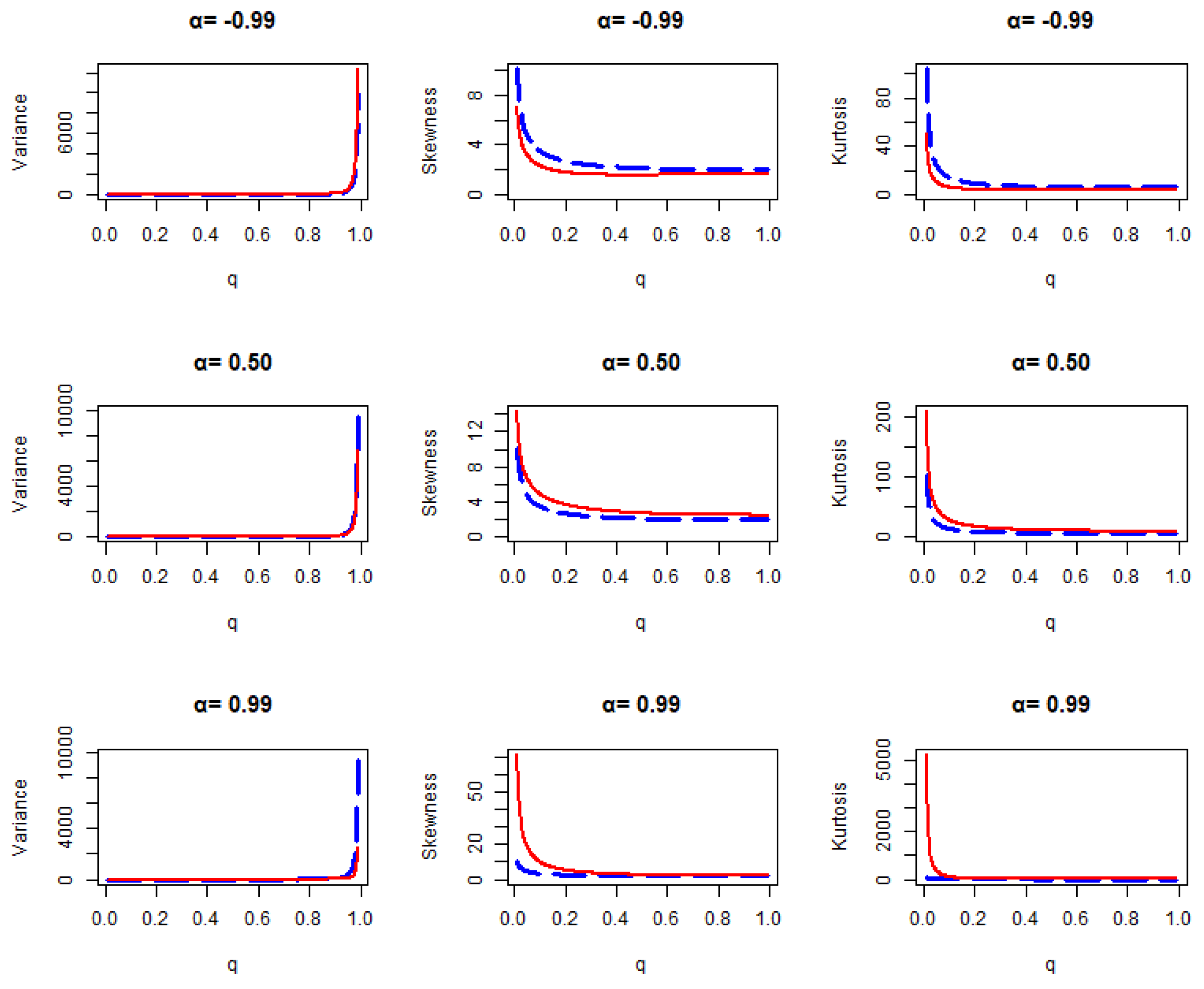
Figure 1.
Variance, skewness, and kurtosis plot for geometric distribution (blue line) and transmuted geometric distribution (red line) for various values of .
Figure 1.
Variance, skewness, and kurtosis plot for geometric distribution (blue line) and transmuted geometric distribution (red line) for various values of .
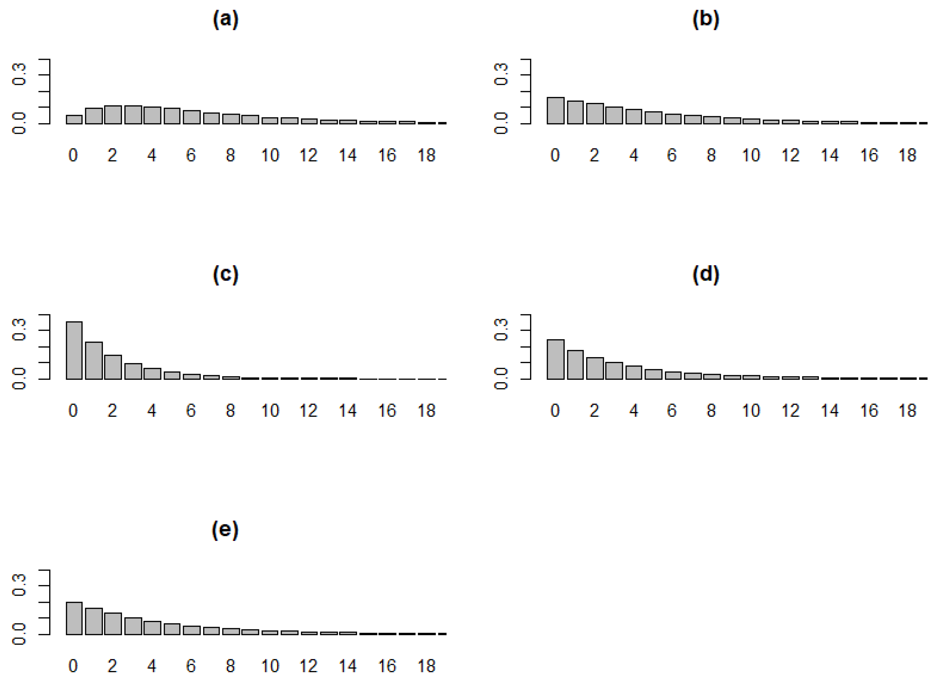
Figure 2.
TGD model with a fixed value of q = 0.6 and various values of . (a) , (b) , (c) , (d) , (e) .
Figure 2.
TGD model with a fixed value of q = 0.6 and various values of . (a) , (b) , (c) , (d) , (e) .
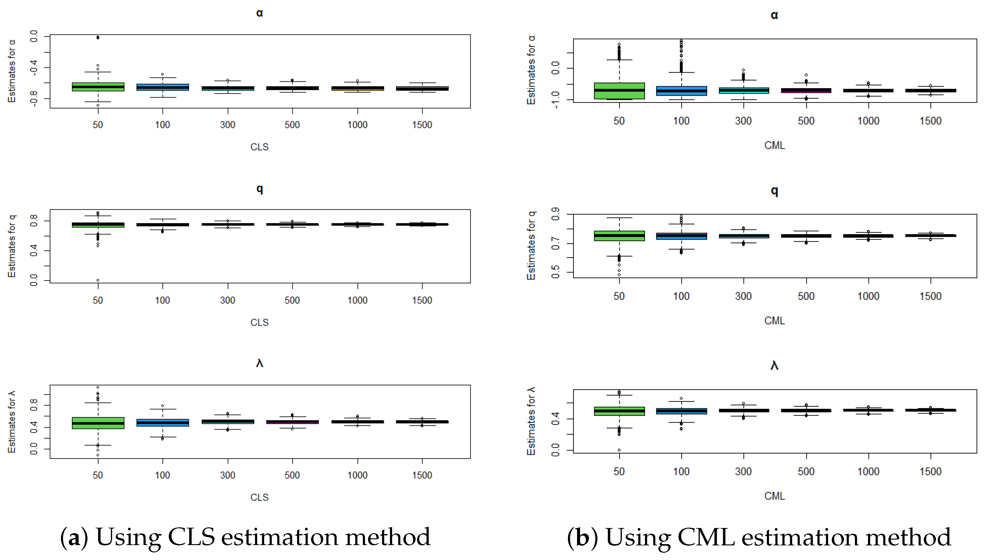
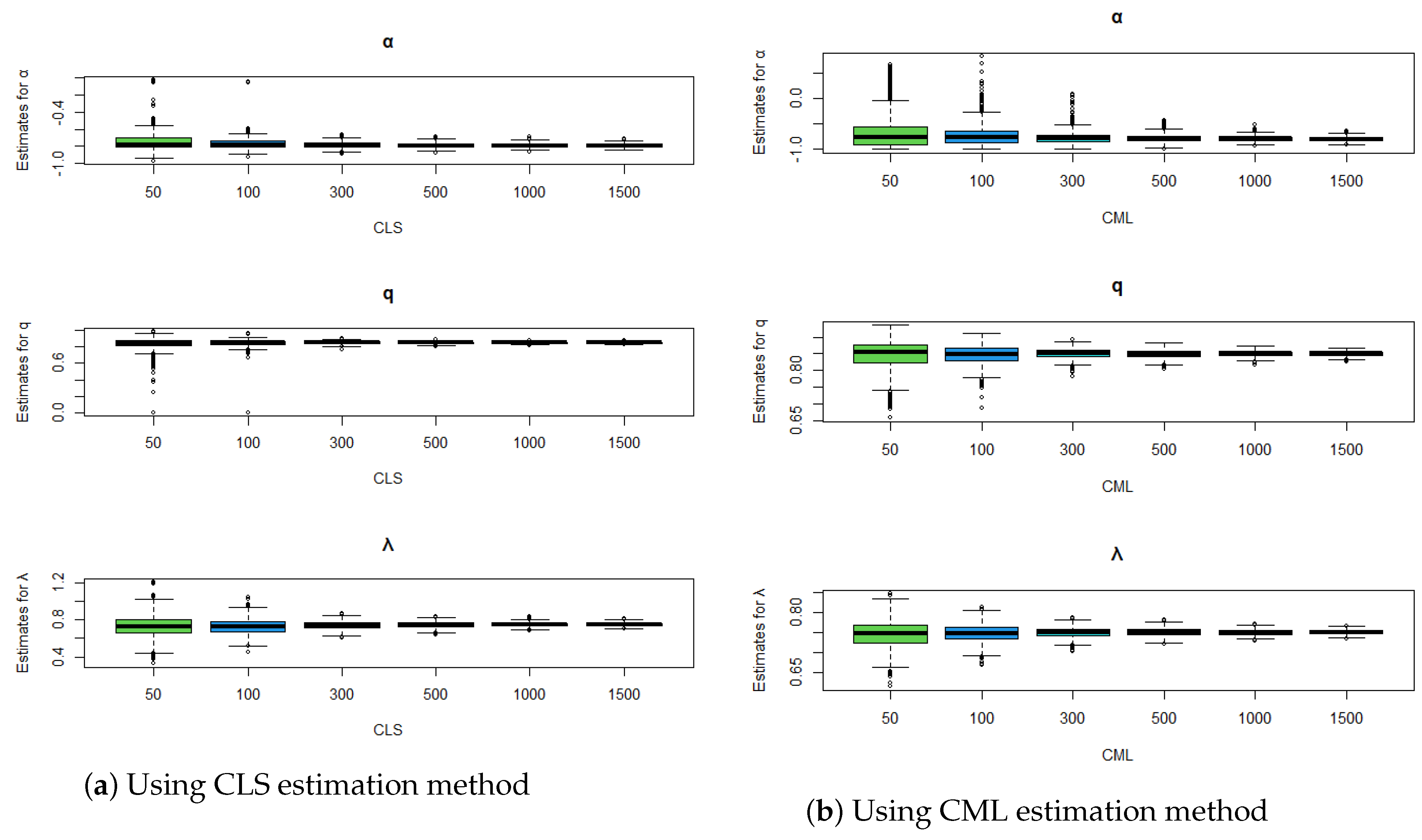
Figure 3.
Comparison of estimation methods using boxplots for , , and .
Figure 3.
Comparison of estimation methods using boxplots for , , and .
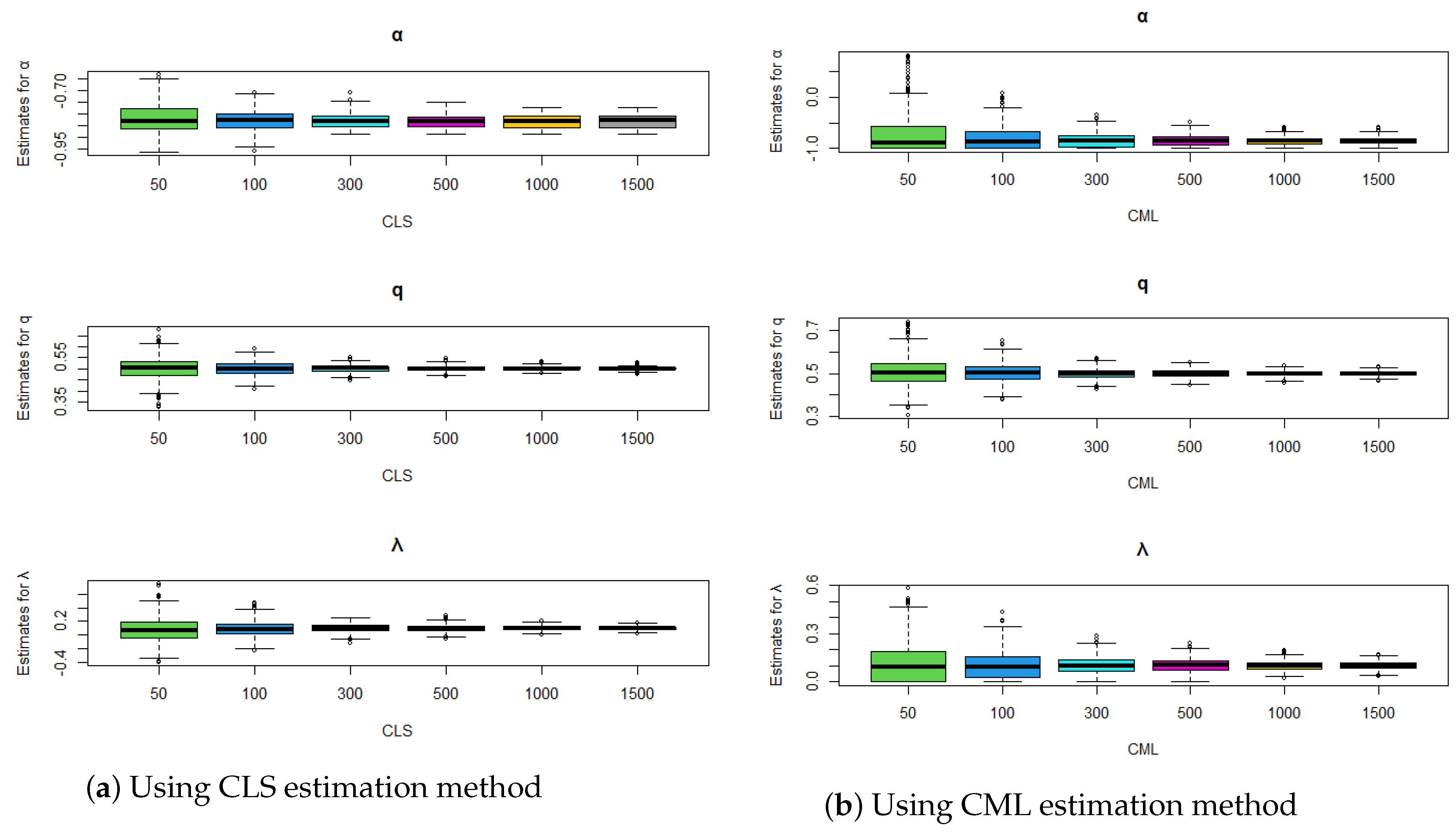
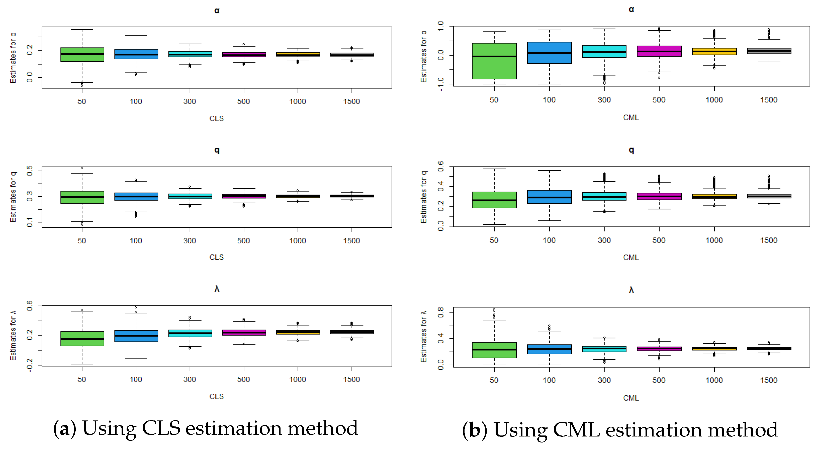
Figure 4.
Comparison of estimation methods using boxplots for , , and .
Figure 4.
Comparison of estimation methods using boxplots for , , and .
Figure 5.
Comparison of estimation methods using boxplots for , , and .
Figure 5.
Comparison of estimation methods using boxplots for , , and .
Figure 6.
Comparison of estimation methods using boxplots for , , and .
Figure 6.
Comparison of estimation methods using boxplots for , , and .
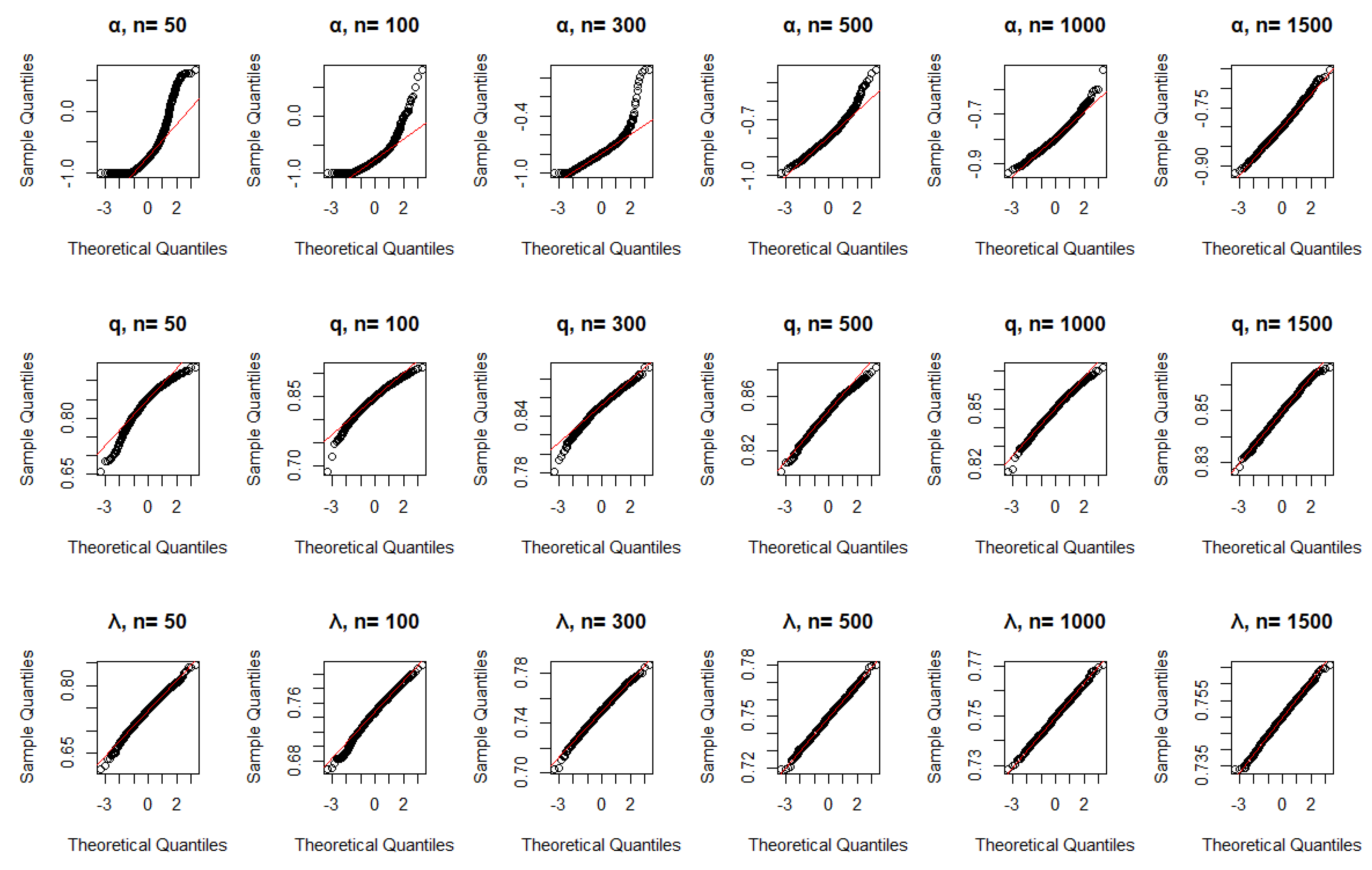
Figure 7.
QQ plots using CML for , , and .
Figure 7.
QQ plots using CML for , , and .
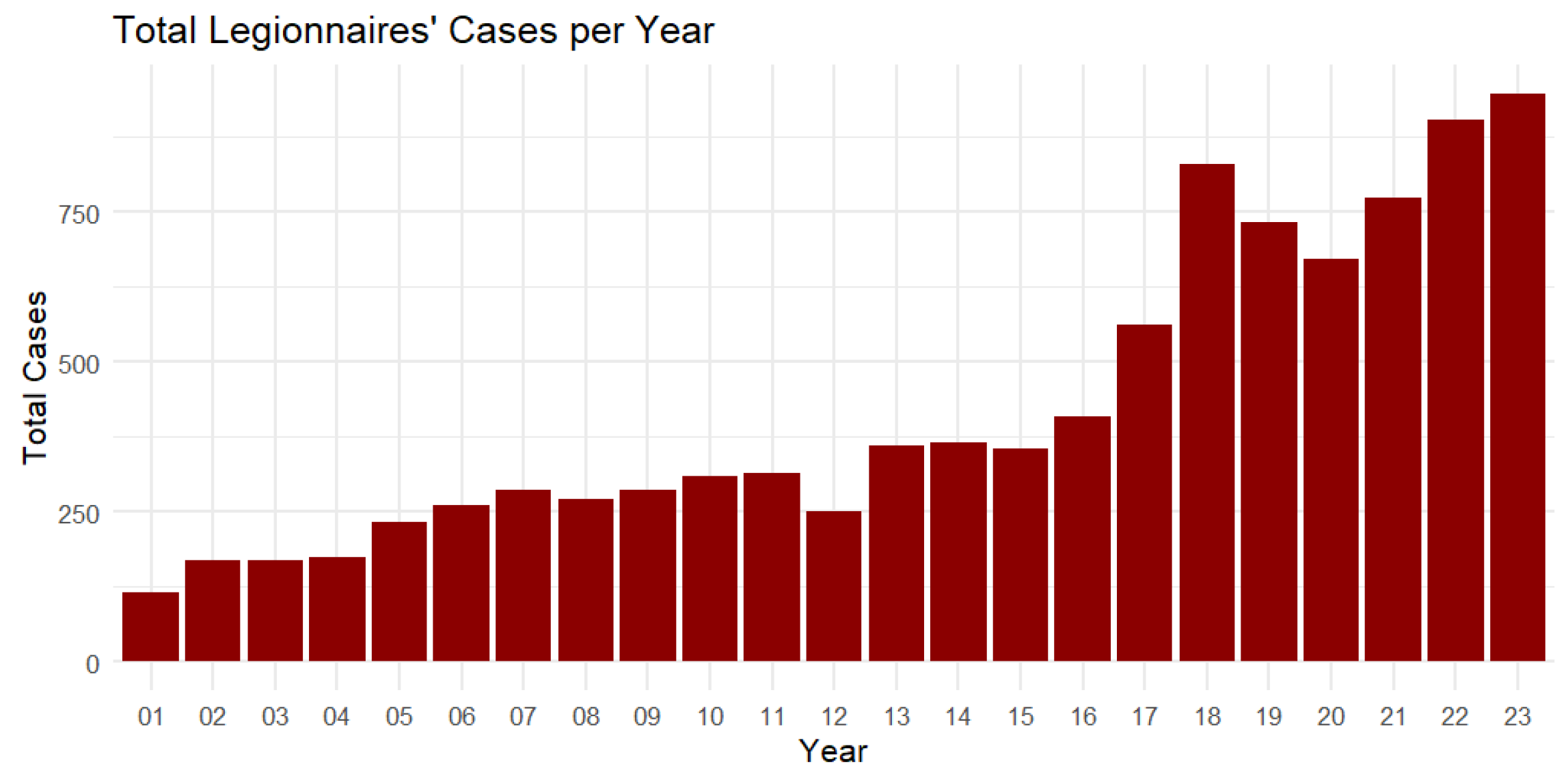
Figure 8.
Total Legionnaires’ cases per year from 2001 to 2023.
Figure 8.
Total Legionnaires’ cases per year from 2001 to 2023.
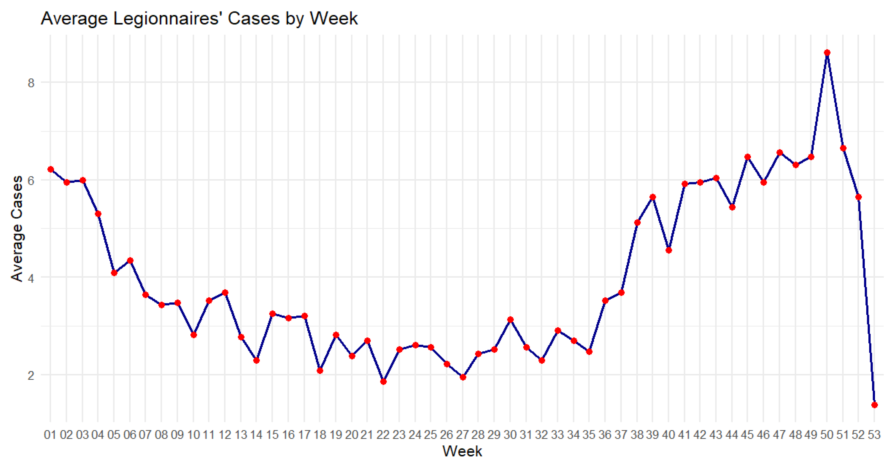
Figure 9.
Average Legionnaires’ cases by week from 2001 to 2023.
Figure 9.
Average Legionnaires’ cases by week from 2001 to 2023.
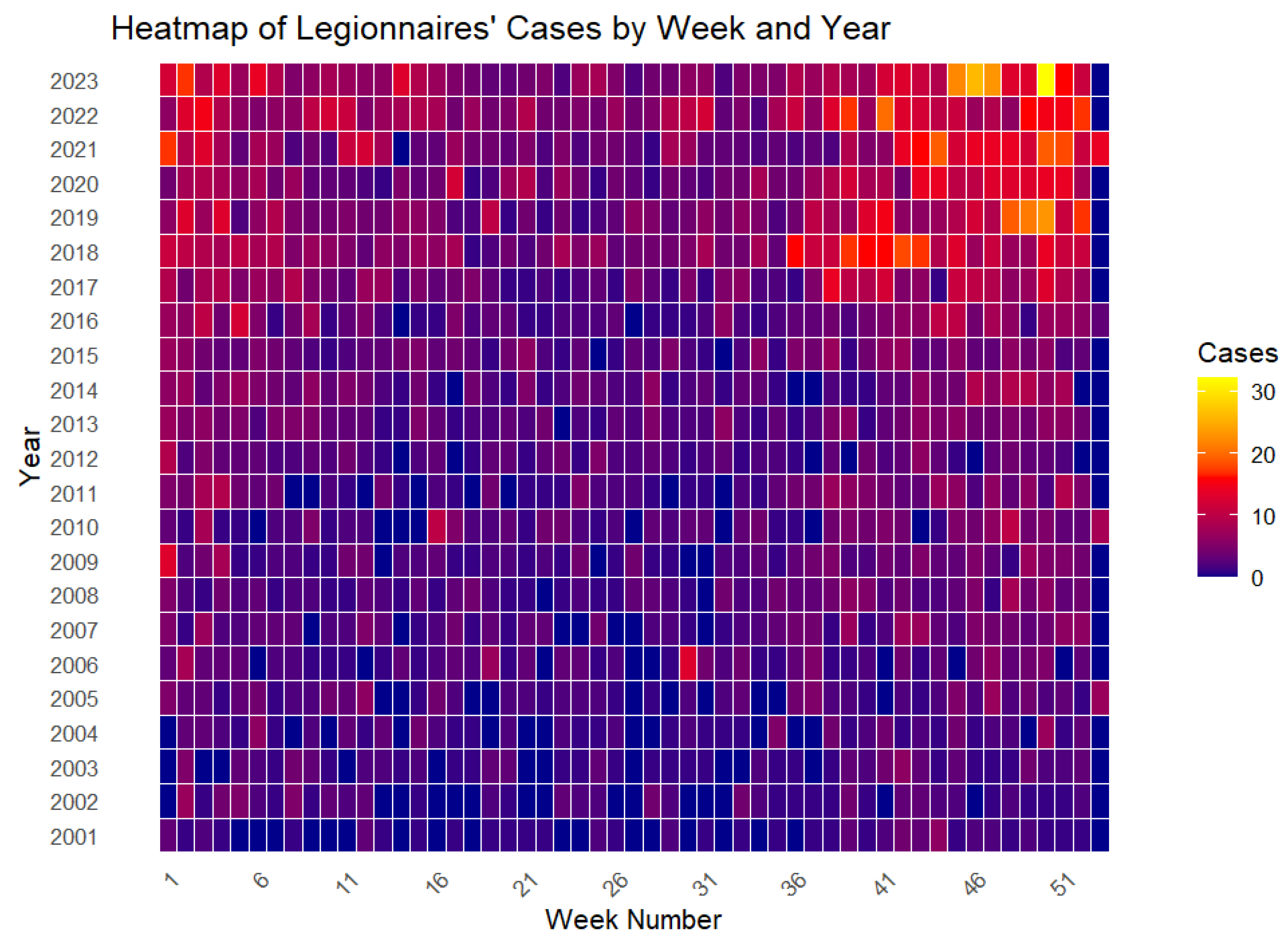
Figure 10.
Heatmap of Legionnaires’ cases by week and year from 2001 to 2023.
Figure 10.
Heatmap of Legionnaires’ cases by week and year from 2001 to 2023.
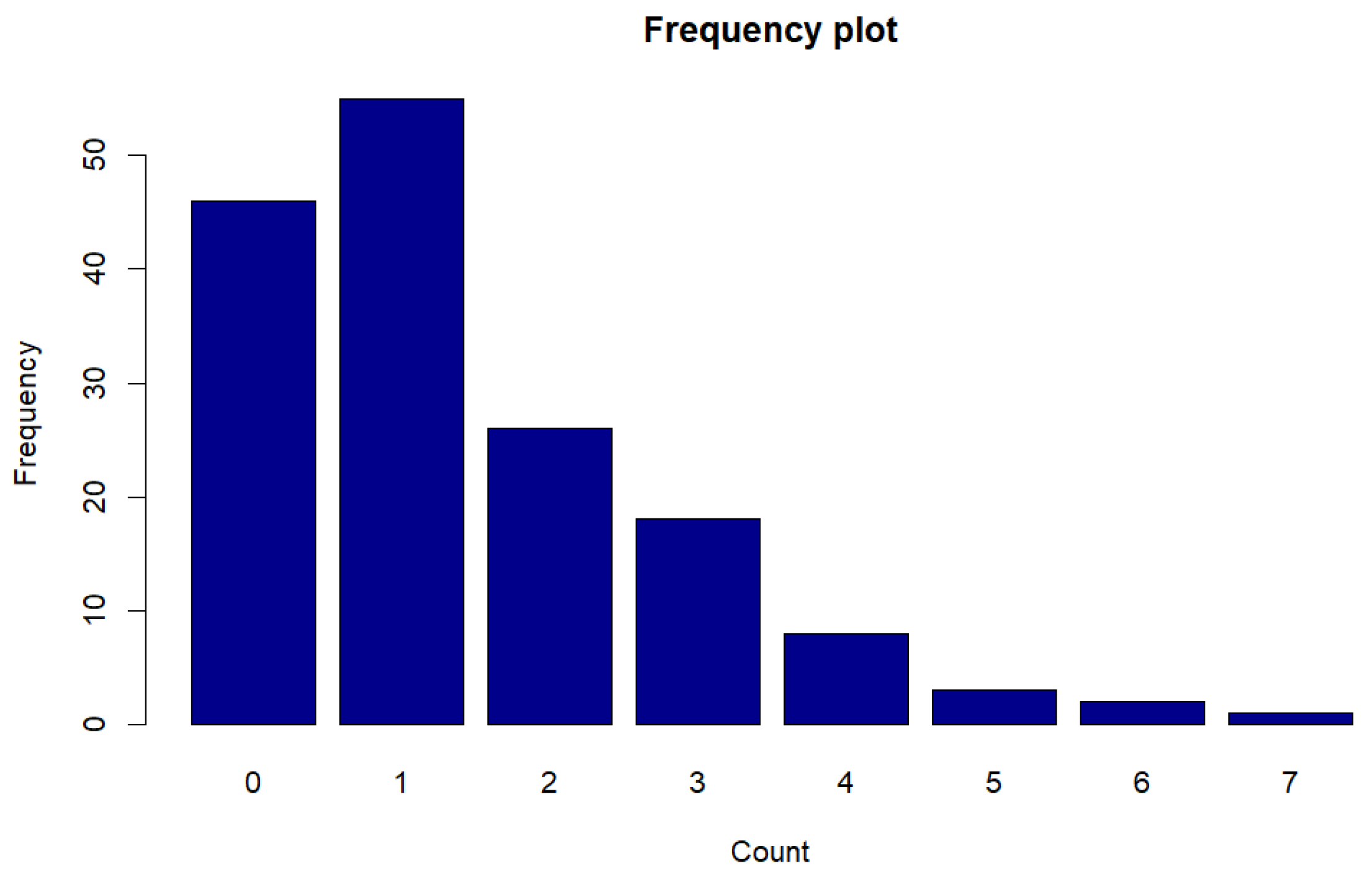
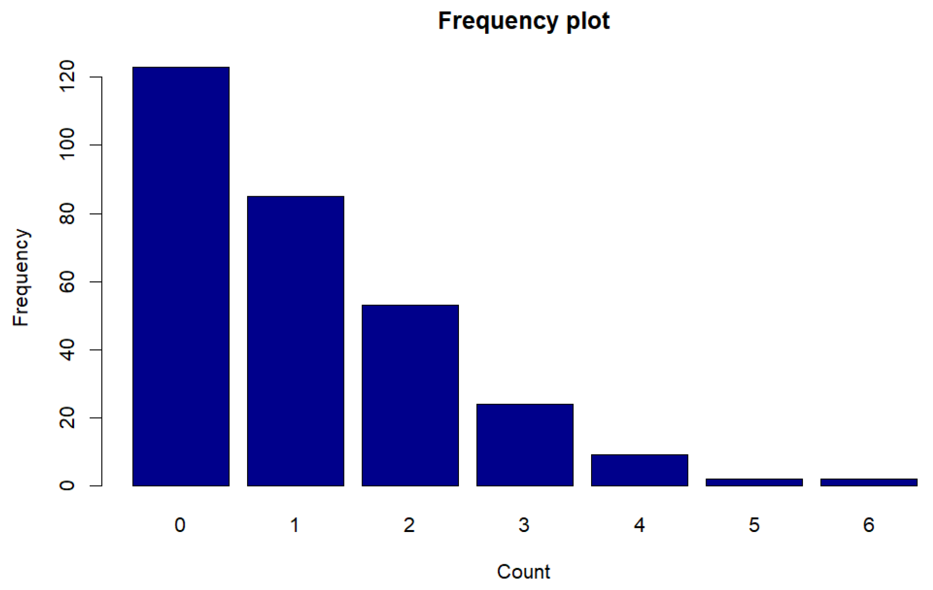
Figure 11.
Frequency plot of counts for Legionnaires disease data.
Figure 11.
Frequency plot of counts for Legionnaires disease data.
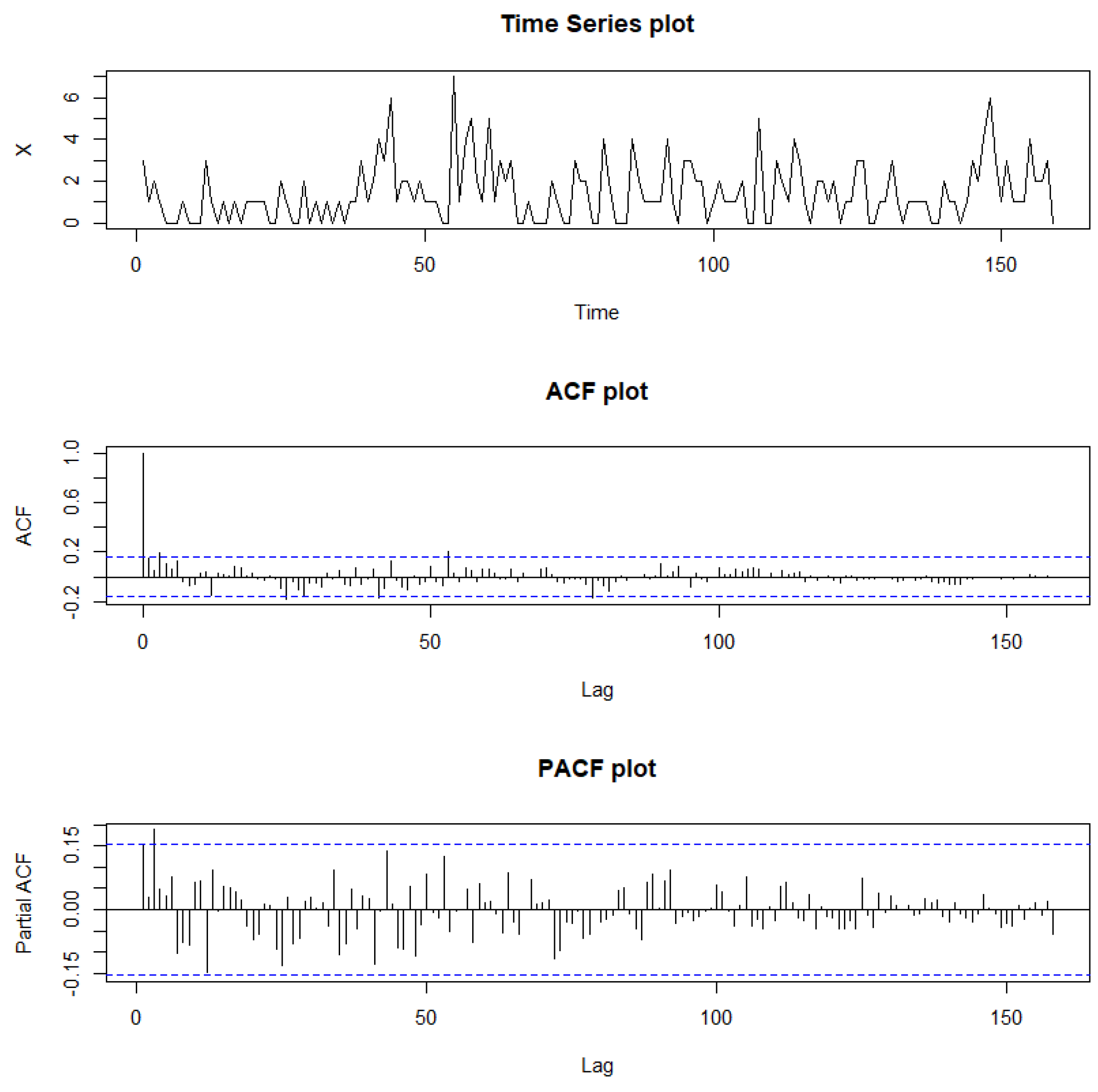
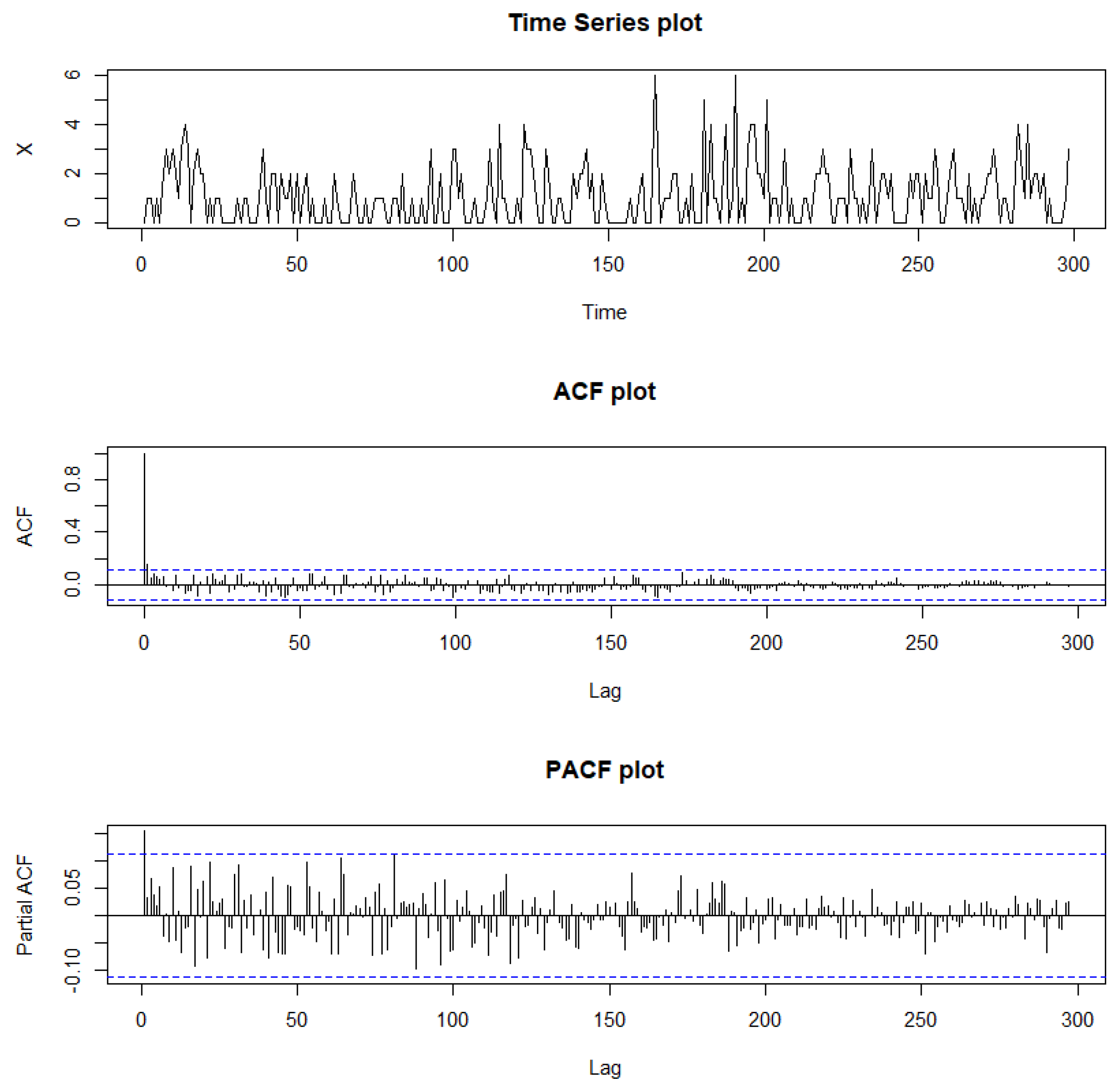
Figure 12.
Sample path, sample ACF, and sample PACF plots for Legionnaires’ disease data.
Figure 12.
Sample path, sample ACF, and sample PACF plots for Legionnaires’ disease data.
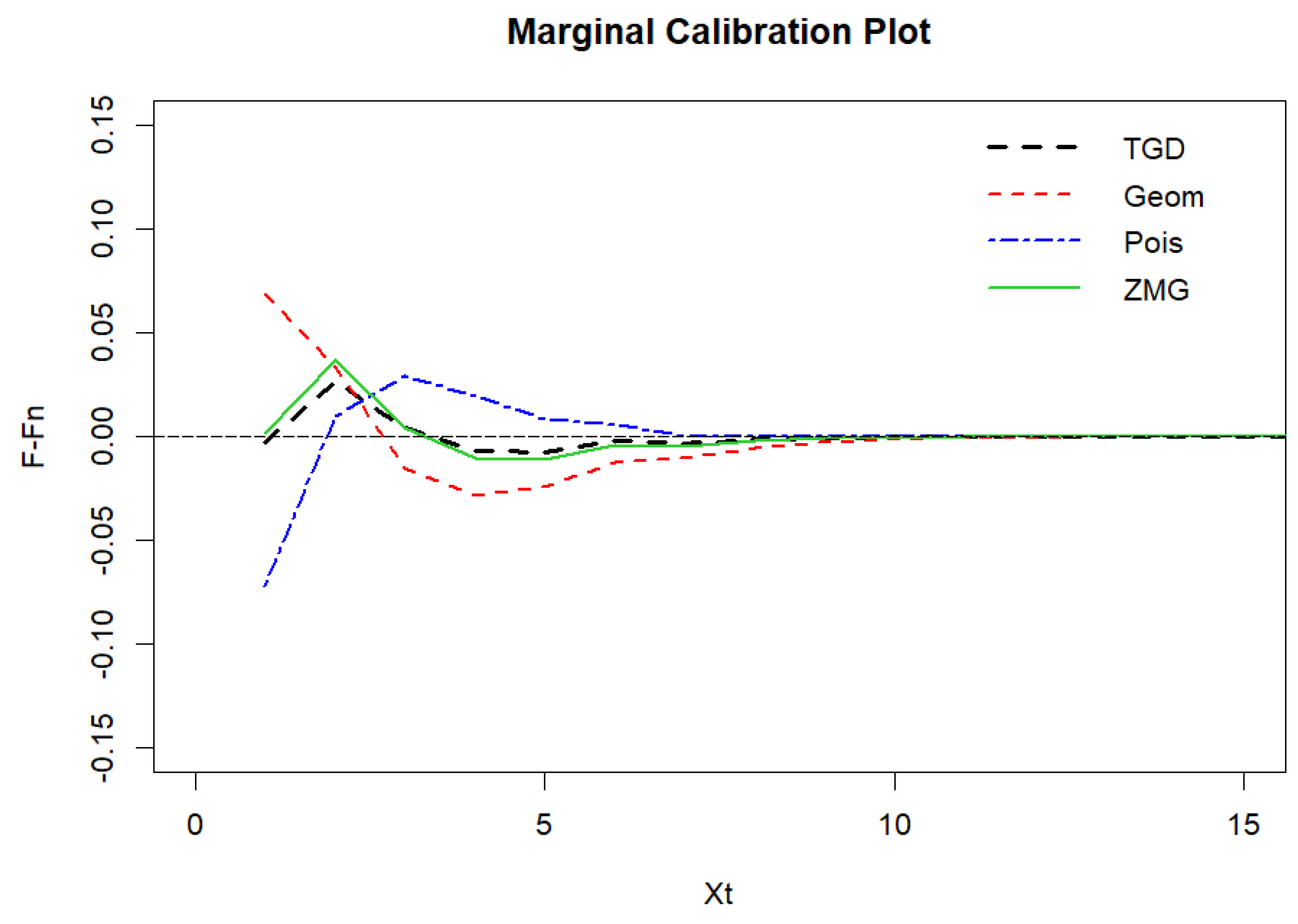
Figure 13.
Marginal calibration plot of Legionnaires’ disease data.
Figure 13.
Marginal calibration plot of Legionnaires’ disease data.
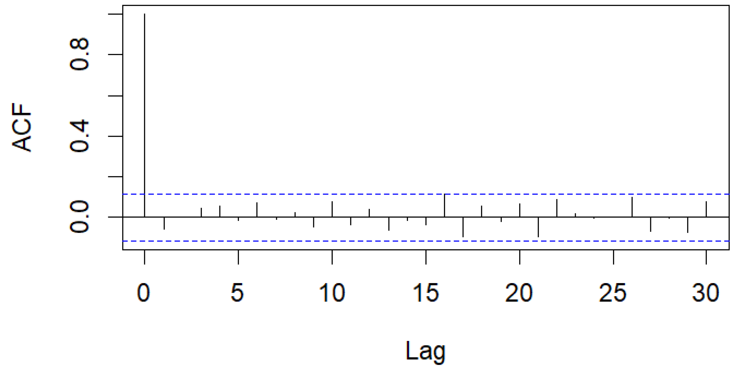
Figure 14.
Sample ACF of Pearson residuals for Legionnaires’ disease data.
Figure 14.
Sample ACF of Pearson residuals for Legionnaires’ disease data.
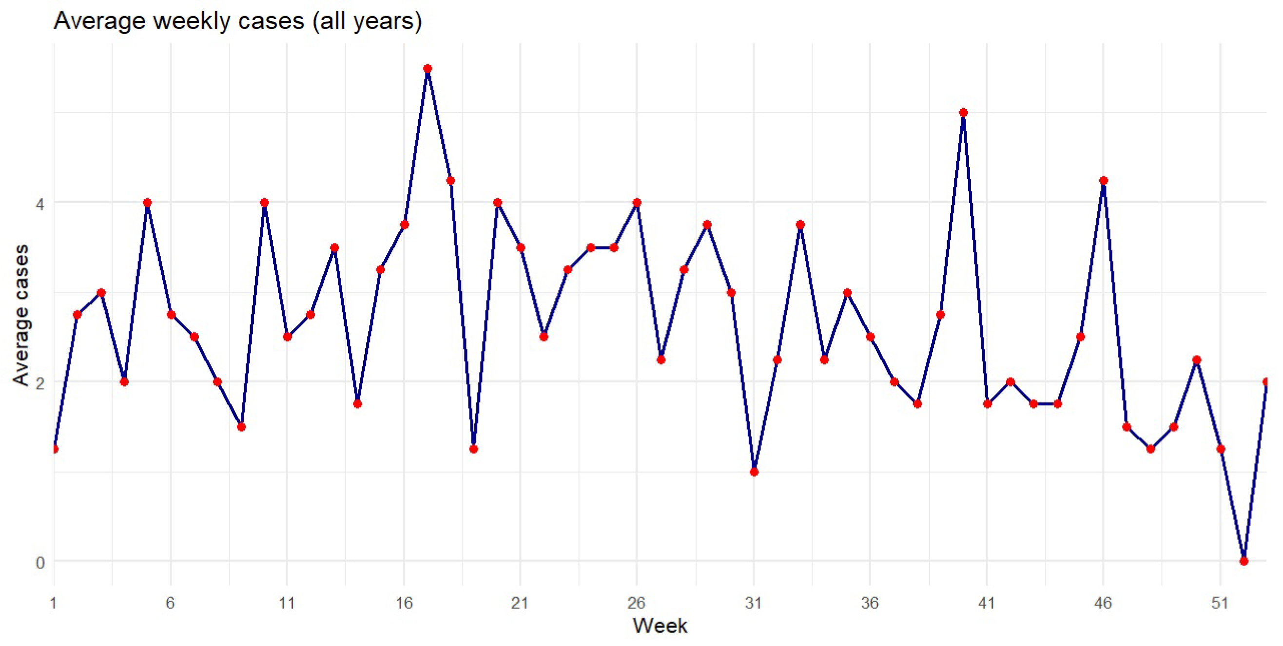
Figure 15.
Average syphilis cases by week from 2007 to 2010.
Figure 15.
Average syphilis cases by week from 2007 to 2010.
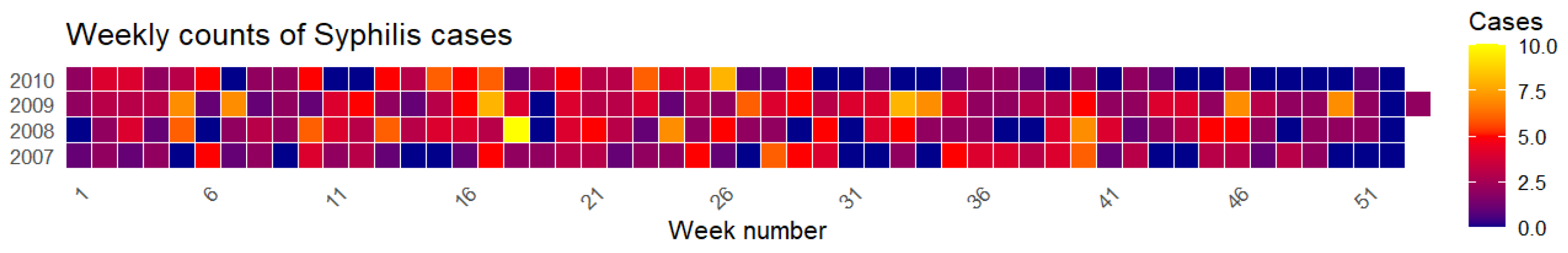
Figure 16.
Heatmap of syphilis cases by week and year from 2007 to 2010.
Figure 16.
Heatmap of syphilis cases by week and year from 2007 to 2010.
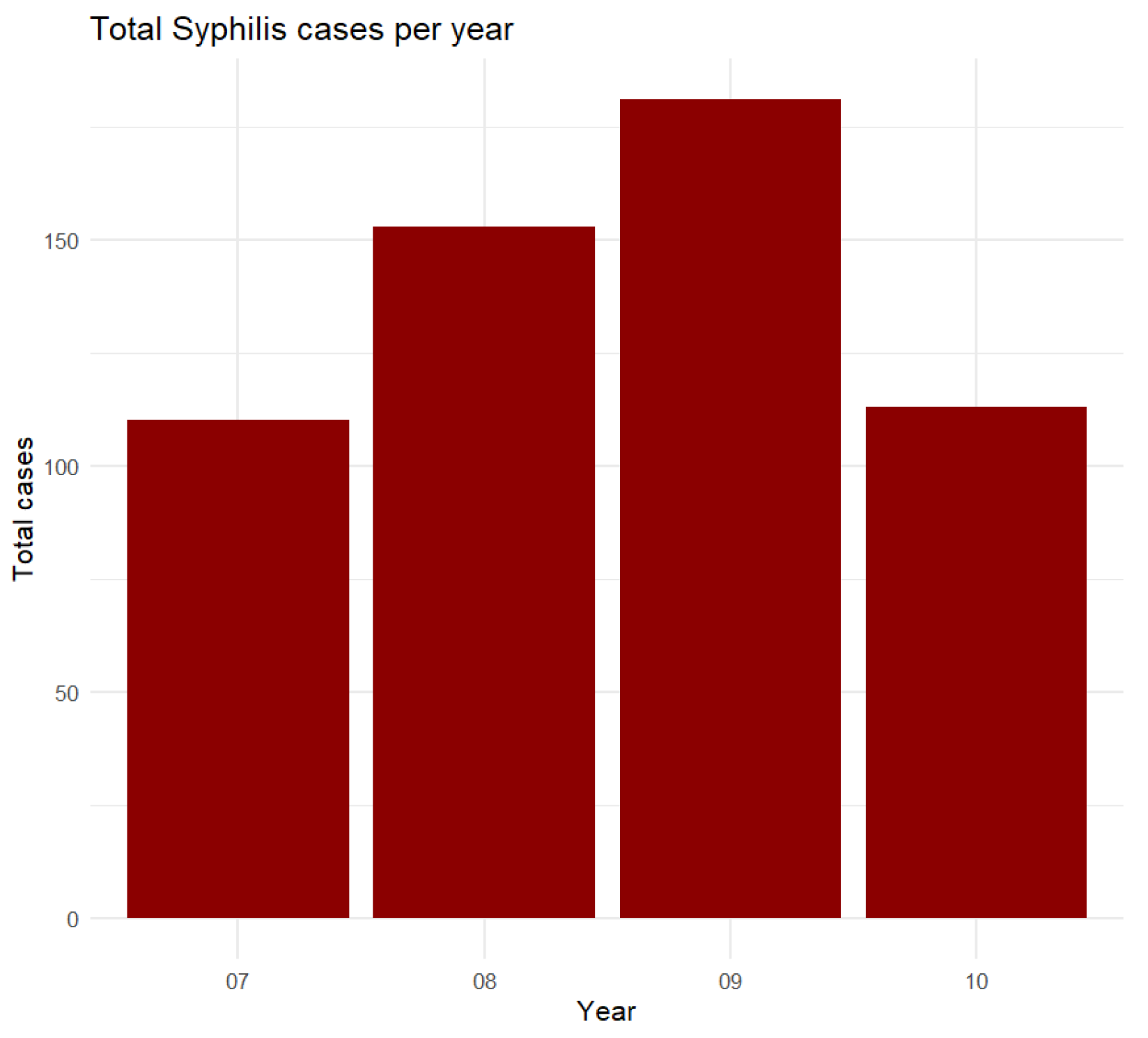
Figure 17.
Total syphilis cases per year from 2007 to 2010.
Figure 17.
Total syphilis cases per year from 2007 to 2010.
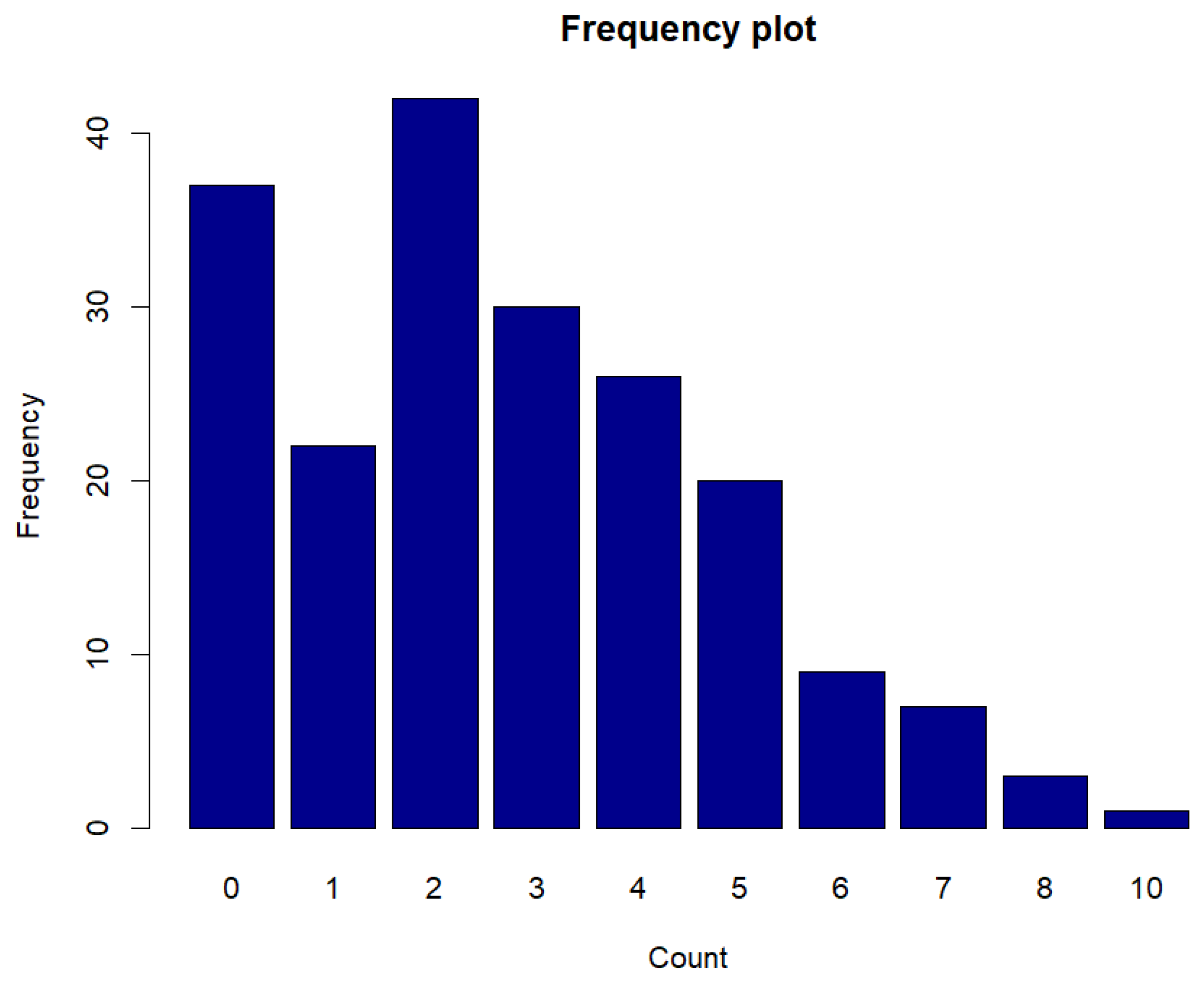
Figure 18.
Frequency plot of counts for syphilis cases.
Figure 18.
Frequency plot of counts for syphilis cases.
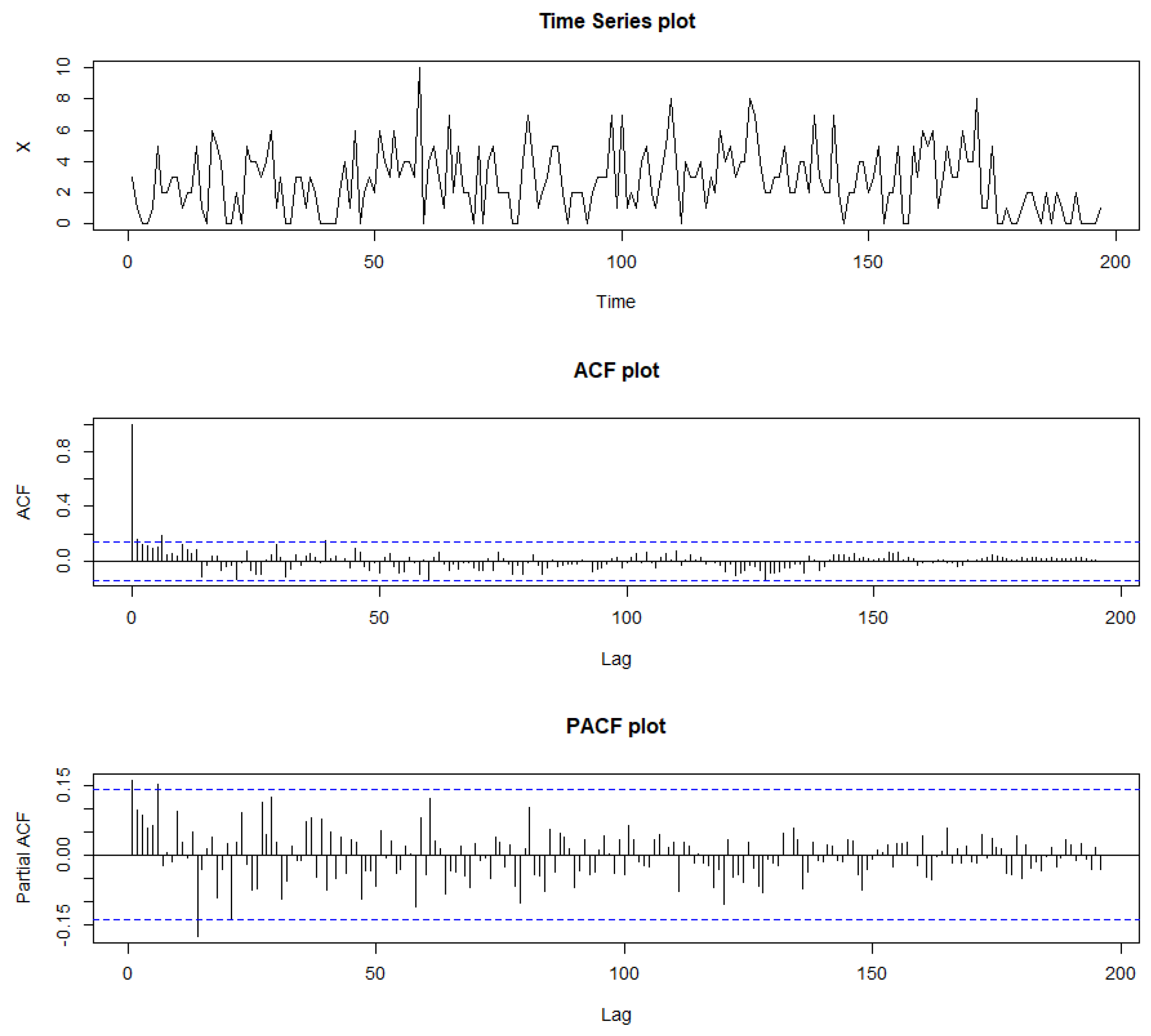
Figure 19.
Sample path, sample ACF, and sample PACF plots for syphilis cases.
Figure 19.
Sample path, sample ACF, and sample PACF plots for syphilis cases.
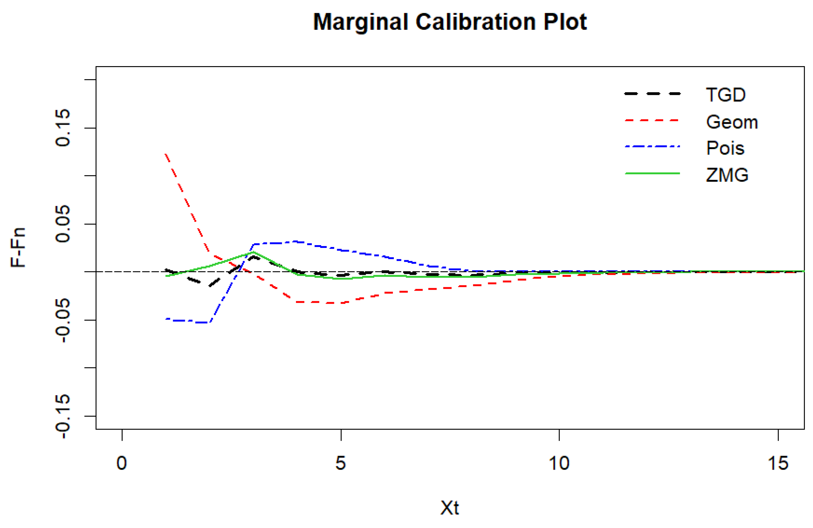
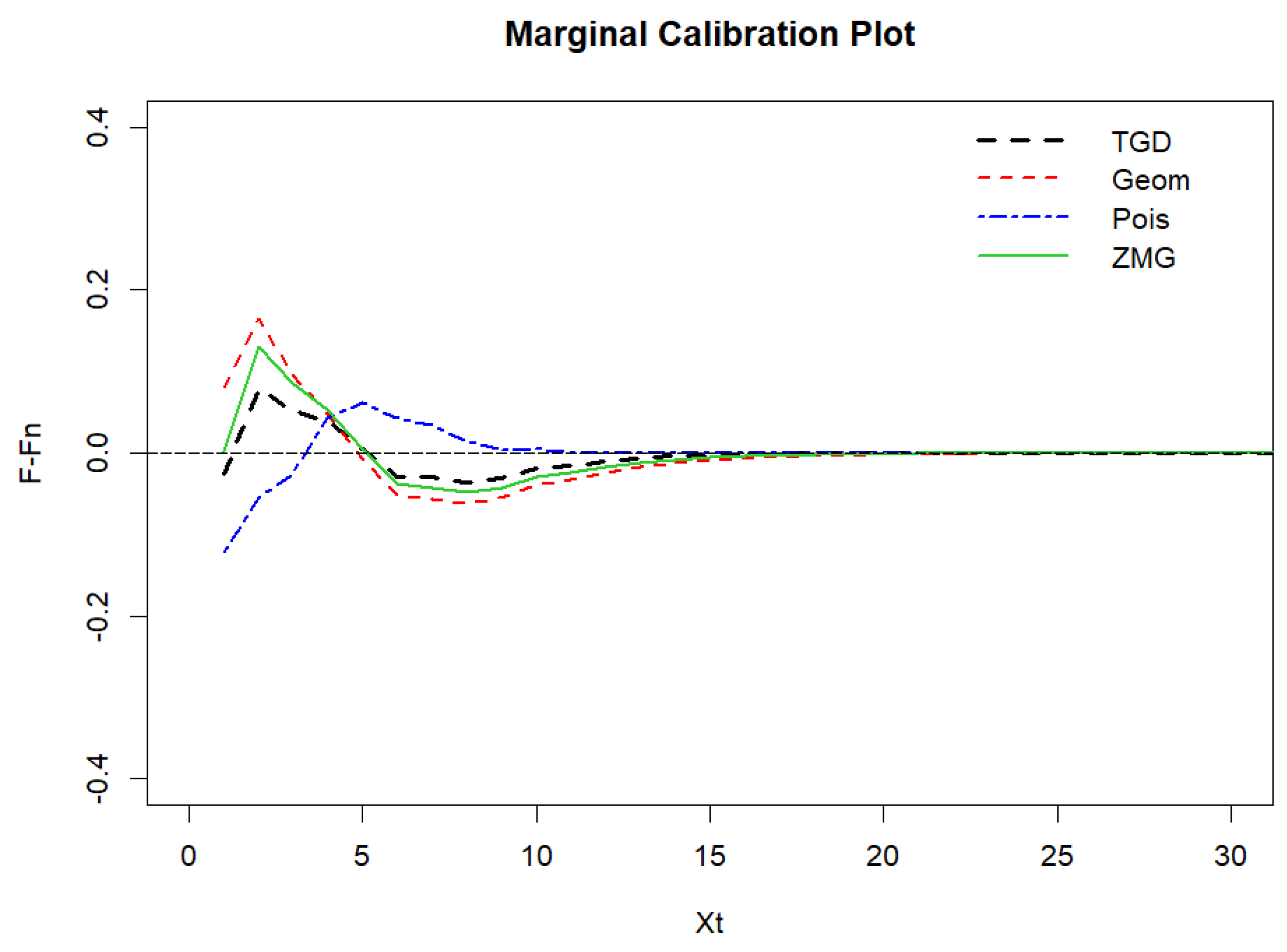
Figure 20.
Marginal calibration plot of syphilis cases.
Figure 20.
Marginal calibration plot of syphilis cases.
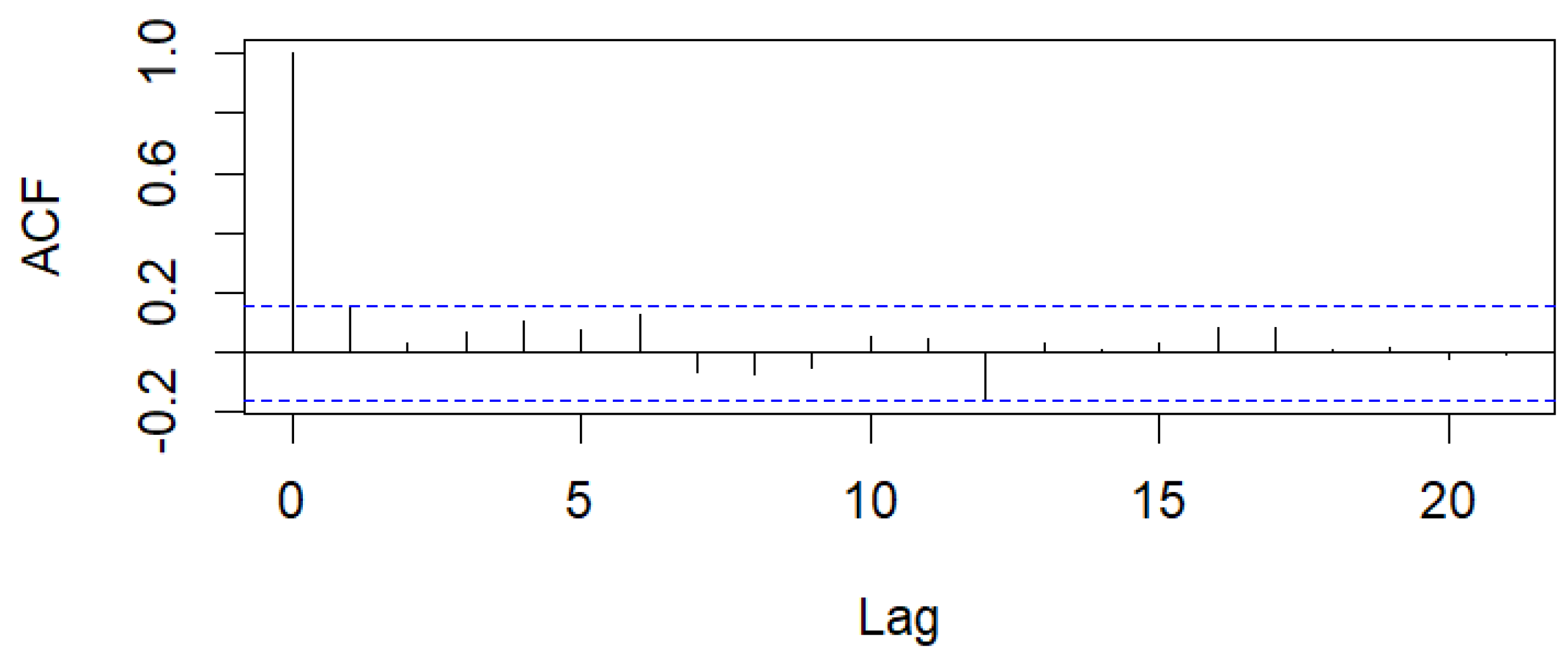
Figure 21.
Sample ACF of Pearson residuals for syphilis cases.
Figure 21.
Sample ACF of Pearson residuals for syphilis cases.
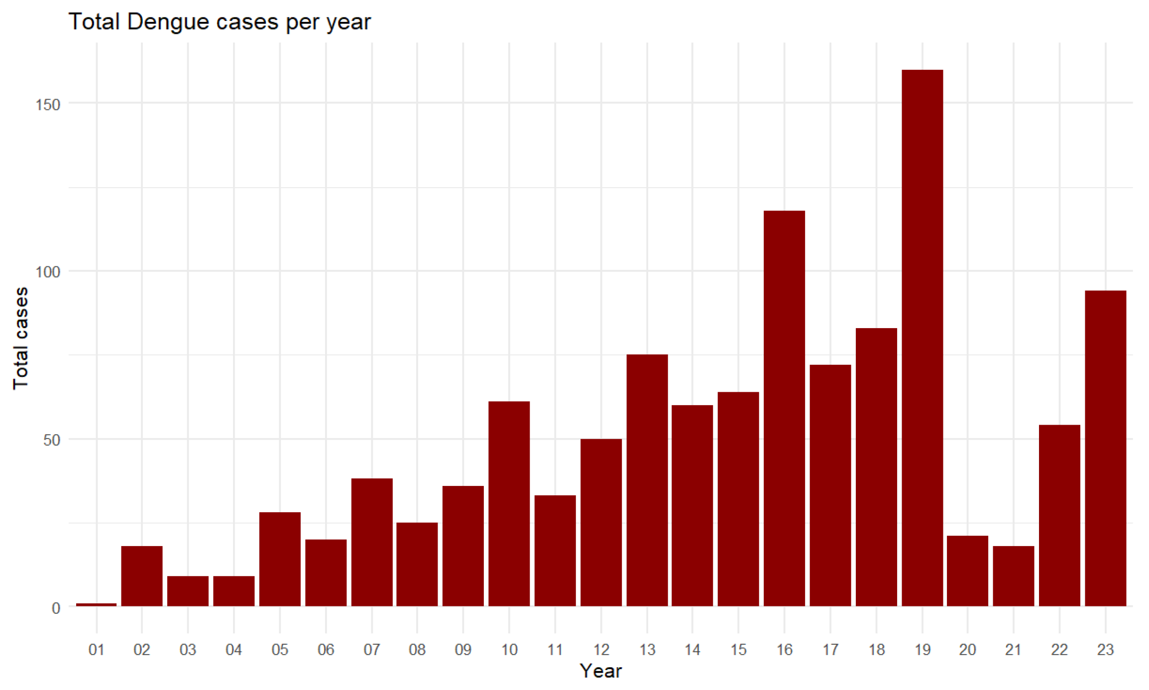
Figure 22.
Total Dengue cases per year from 2001 to 2023.
Figure 22.
Total Dengue cases per year from 2001 to 2023.
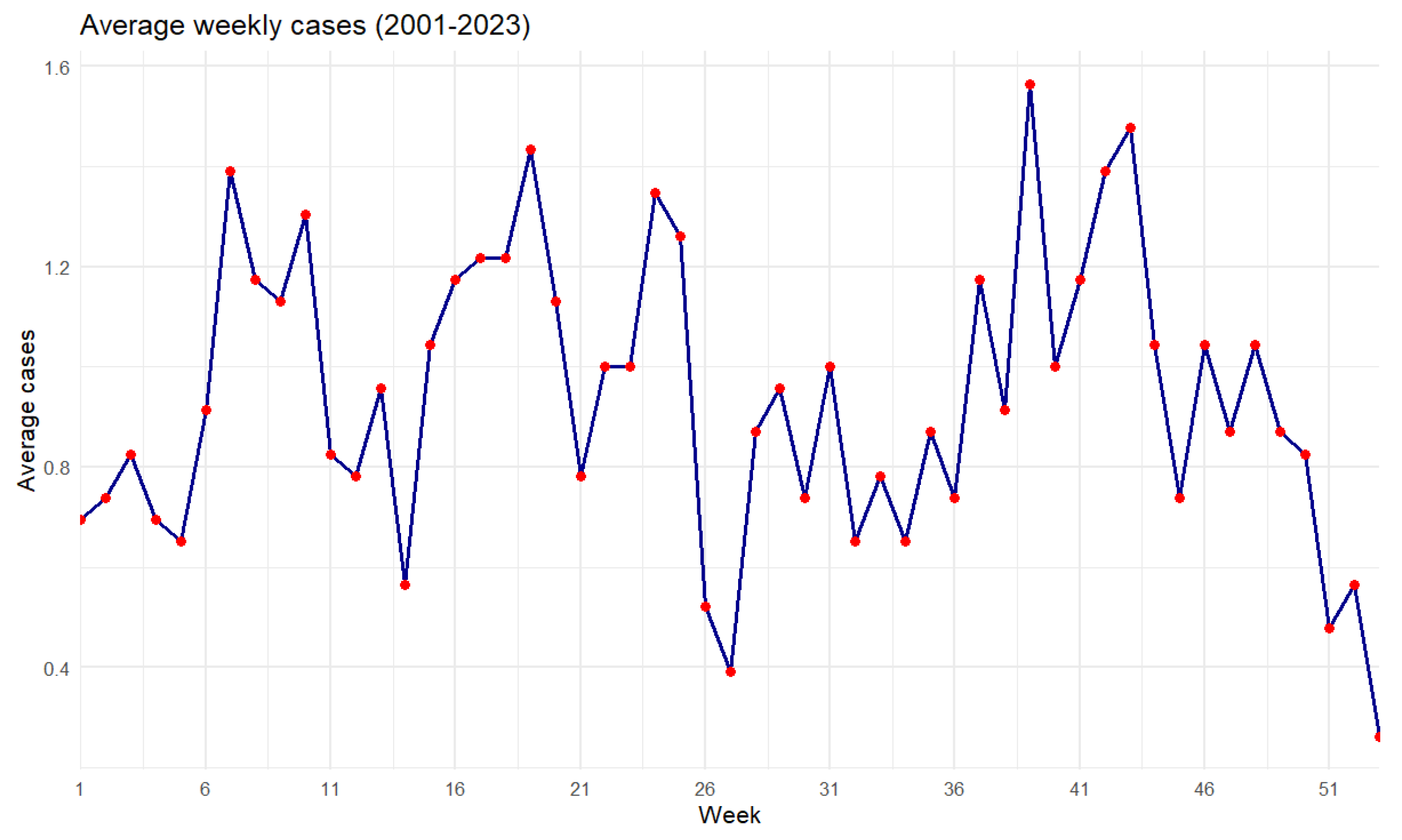
Figure 23.
Average dengue cases by week from 2001 to 2023.
Figure 23.
Average dengue cases by week from 2001 to 2023.
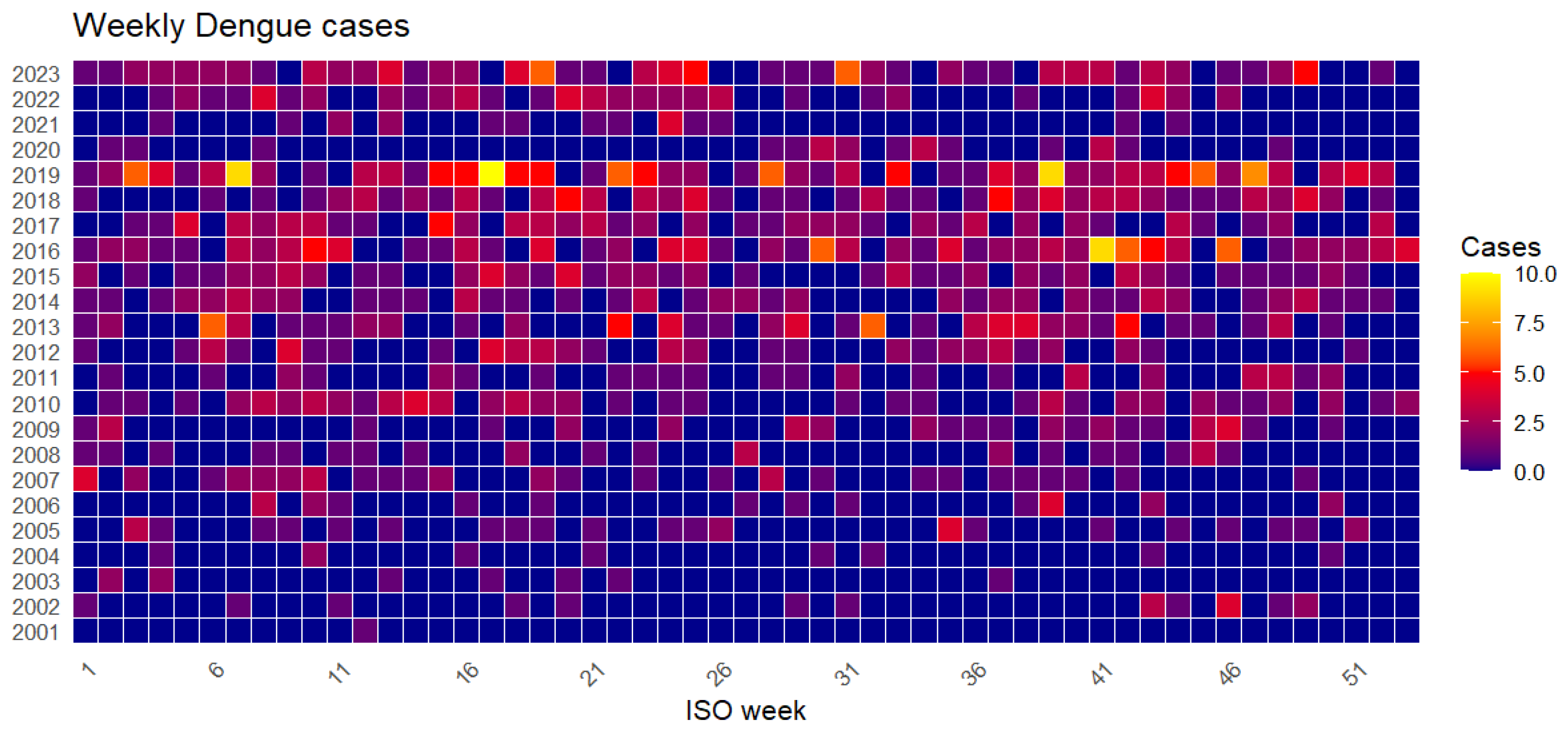
Figure 24.
Heatmap of dengue cases by week and year from 2001 to 2023.
Figure 24.
Heatmap of dengue cases by week and year from 2001 to 2023.
Figure 25.
Frequency plot of counts for dengue disease data.
Figure 25.
Frequency plot of counts for dengue disease data.
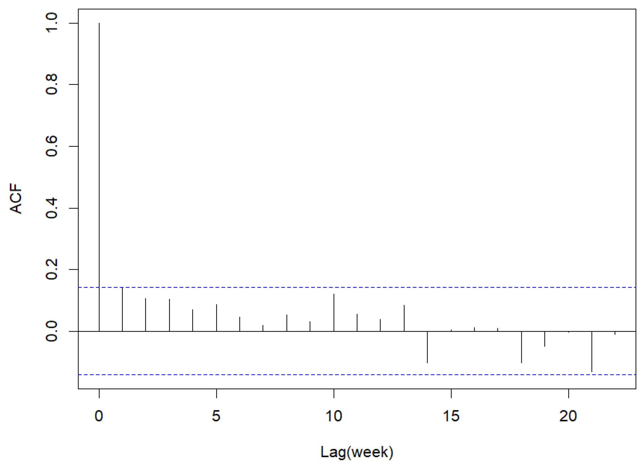
Figure 26.
Sample path, sample ACF, and sample PACF plots for dengue disease data.
Figure 26.
Sample path, sample ACF, and sample PACF plots for dengue disease data.
Figure 27.
Marginal calibration plot of dengue disease data.
Figure 27.
Marginal calibration plot of dengue disease data.
Figure 28.
Sample ACF of Pearson residuals for dengue disease data.
Figure 28.
Sample ACF of Pearson residuals for dengue disease data.
Table 1.
Parameter estimates and their mean squared errors.
Table 1.
Parameter estimates and their mean squared errors.
| n | | | | | | |
|---|
| | , , |
| 50 | | | | | | |
| | () | () | () | () | () | () |
| 100 | | | | | | |
| | () | () | () | () | () | () |
| 300 | | | | | | |
| | () | () | () | () | () | () |
| 500 | | | | | | |
| | () | () | () | () | () | () |
| 1000 | | | | | | |
| | () | () | () | () | () | () |
| 1500 | | | | | | |
| | () | () | () | () | () | () |
Table 2.
AIC and BIC for the seasonal INAR(1) models for Legionnaires’ disease data.
Table 2.
AIC and BIC for the seasonal INAR(1) models for Legionnaires’ disease data.
| Model | Estimated Values | AIC | BIC | RMSE |
|---|
| PoINAR(1)s | , | 505.0183 | 511.1561 | 1.3887 |
| GINAR(1)s | , | 514.1081 | 520.2459 | 1.3939 |
| NGINAR(1)s | , | 513.2207 | 519.3585 | 1.3876 |
| ZMGINAR(1)s | , , | 506.1553 | 515.3620 | 1.4088 |
| TGDINAR(1)s | , , | 498.3401 | 507.5468 | 1.3902 |
Table 3.
Point forecast for Legionnaires’ disease data with = 0.90.
Table 3.
Point forecast for Legionnaires’ disease data with = 0.90.
| k | | Mean | Mode | Median | HPP |
|---|
| 1 | 1 | 1.72 | 1 | 1 | [0, 4) |
| 2 | 3 | 1.96 | 1 | 2 | [0, 4) |
| 3 | 1 | 1.60 | 1 | 1 | [0, 4) |
| 4 | 1 | 1.41 | 1 | 1 | [0, 3) |
| 5 | 1 | 1.44 | 1 | 1 | [0, 3) |
| 6 | 4 | 1.41 | 1 | 1 | [0, 3) |
| 7 | 2 | 1.42 | 1 | 1 | [0, 3) |
| 8 | 2 | 1.42 | 1 | 1 | [0, 3) |
| 9 | 3 | 1.42 | 1 | 1 | [0, 3) |
| 10 | 0 | 1.42 | 1 | 1 | [0, 3) |
Table 4.
AIC and BIC for the seasonal INAR(1) models for syphilis cases.
Table 4.
AIC and BIC for the seasonal INAR(1) models for syphilis cases.
| Model | Estimated Values | AIC | BIC | RMSE |
|---|
| PoINAR(1)s | , | 820.7281 | 827.2945 | 2.0338 |
| GINAR(1)s | , | 833.4564 | 840.0229 | 2.0413 |
| NGINAR(1)s | , | 828.0160 | 834.5824 | 2.0591 |
| ZMGINAR(1)s | , , | 825.2454 | 835.0950 | 2.0664 |
| TGDINAR(1)s | , , | 806.4264 | 816.2760 | 2.0332 |
Table 5.
Point forecast for syphilis cases with = 0.90.
Table 5.
Point forecast for syphilis cases with = 0.90.
| k | | Mean | Mode | Median | HPP |
|---|
| 1 | 2 | 2.74 | 1 | 2 | [0, 6) |
| 2 | 1 | 2.74 | 1 | 2 | [0, 6) |
| 3 | 0 | 2.68 | 1 | 2 | [0, 6) |
| 4 | 0 | 2.61 | 1 | 2 | [0, 6) |
| 5 | 2 | 2.74 | 1 | 2 | [0, 6) |
| 6 | 0 | 2.61 | 1 | 2 | [0, 6) |
| 7 | 0 | 2.79 | 1 | 2 | [0, 6) |
| 8 | 0 | 2.79 | 1 | 2 | [0, 6) |
| 9 | 0 | 2.79 | 1 | 2 | [0, 6) |
| 10 | 1 | 2.78 | 1 | 2 | [0, 6) |
Table 6.
AIC and BIC for the seasonal INAR(1) models for dengue disease data.
Table 6.
AIC and BIC for the seasonal INAR(1) models for dengue disease data.
| Model | Estimated Values | AIC | BIC | RMSE |
|---|
| PoINAR(1)s | , | 850.0882 | 857.4824 | 1.1896 |
| GINAR(1)s | , | 855.7436 | 863.1378 | 1.1909 |
| NGINAR(1)s | , | 852.6276 | 860.0218 | 1.1916 |
| ZMGINAR(1)s | , , | 849.2594 | 860.3507 | 1.2194 |
| TGDINAR(1)s | , , | 840.0040 | 851.0953 | 1.1893 |
Table 7.
Point forecast for dengue disease data with = 0.90.
Table 7.
Point forecast for dengue disease data with = 0.90.
| k | | Mean | Mode | Median | HPP |
|---|
| 1 | 1 | 1.22 | 1 | 1 | [0, 3) |
| 2 | 2 | 1.10 | 0 | 1 | [0, 3) |
| 3 | 0 | 1.09 | 0 | 1 | [0, 3) |
| 4 | 1 | 1.08 | 0 | 1 | [0, 3) |
| 5 | 0 | 1.08 | 0 | 1 | [0, 3) |
| 6 | 0 | 1.08 | 0 | 1 | [0, 3) |
| 7 | 0 | 1.08 | 0 | 1 | [0, 3) |
| 8 | 0 | 1.08 | 0 | 1 | [0, 3) |
| 9 | 1 | 1.08 | 0 | 1 | [0, 3) |
| 10 | 3 | 1.08 | 0 | 1 | [0, 3) |


 ,
, 
