Article

Application of Log-Type Estimators for Addressing Non-Response in Survey Sampling Using Real Datasets

1
Department of Mathematics, School of Advanced Sciences, VIT-AP University, Inavolu, Beside AP Secretariat, Amaravati AP-522237, India
2
Department of Quantitative Methods, School of Business, King Faisal University, Al-Ahsa 31982, Saudi Arabia
*
Authors to whom correspondence should be addressed.
Mathematics 2025, 13(7), 1089; https://doi.org/10.3390/math13071089
Submission received: 12 February 2025 / Revised: 14 March 2025 / Accepted: 24 March 2025 / Published: 26 March 2025
(This article belongs to the Special Issue Applied Statistics in Real-World Problems)

Abstract

:
There is a difficulty in survey sampling when non-response (NR) occurs in the process of estimating the population parameters. This study examines the effectiveness of combined and separate log-type estimators when using bivariate auxiliary information when NR occurs in data. In this study, we propose families of novel log-type estimators under various scenarios. We performed an analysis on the reliability and efficiency of our proposed estimators in situations when NR occurs in both study and auxiliary variables and when NR occurs only in study variables. In this study, we have concentrated on certain issues like how the non-response effects the estimators’ efficiency, how different NR rates effect the precision of estimators, and how the combined and separate types of estimators handle the problem of NR. We proved the efficiency of our proposed estimators by using the bias and mean square error (MSE) metrics under different NR rates, illustrating the positive correlation between higher NR rates and increased errors. To evaluate the impact of NR on MSE values, we took four real datasets, which included a cost of living index dataset for 121 nations and another dataset which is essential for forecasting solar UV radiation hazards influenced by environmental factors, thus enhancing public health awareness and preventive strategies. Additionally, a simulation study comprising 10,000 iterations was also performed. This study provides survey practitioners with valuable guidance on selecting strong estimation methods to enhance the accuracy and efficiency of survey estimates in the context of non-response. This investigation contributes to the domain of survey sampling by demonstrating the robustness and effectiveness of log-type estimators. These estimators enhance survey findings by effectively addressing NR issues.

1. Introduction

Non-response in sample surveys presents a significant obstacle, as it has the potential to create bias and affect the dependability of survey findings. A sample may contain missing data due to factors such as illness, language barriers, participant reluctance, or unavailability during data collection. When conducting surveys on sensitive subjects such as drug use, abortion, or sexually transmitted diseases, non-response (NR) becomes more noticeable, as respondents may opt not to reveal information or decline to participate in the survey entirely. An NR has consequences that go beyond simply missing data. It can result in either underestimating or overestimating demographic metrics, affecting survey results’ reliability. Conventional methods frequently fail to address NR problems or assume that survey data are both complete and unbiased, disregarding the difficulties presented by individuals who do not respond.
Stratified random sampling is an important methodological strategy in survey research that helps deal with the complications caused by NR. Stratified sampling involves dividing the population into homogeneous subgroups, or strata, based on relevant criteria. This method assures that each subgroup is sufficiently represented in the sample. Stratification enhances the accuracy of estimates and allows researchers to customise tactics to minimise NR effects in each stratum. Within each stratum, it is possible to use particular tactics such as targeted follow-ups, alternate contact methods, or weighting adjustments to increase response rates and make up for missing data. These customised approaches are crucial for preserving the accuracy of survey findings, especially when addressing delicate topics that often have higher rates of NR. Furthermore, stratified random sampling allows for incorporating additional data pertaining to each stratum, such as demographic characteristics or past records. By utilising additional data, researchers can more effectively account for bias caused by NR, thus improving the accuracy and dependability of estimates for population parameters.
Many researchers worked on NR. This issue was initially addressed by [1]. Auxiliary information is essential in statistical estimation, as it offers supplementary data that can enhance the accuracy and precision of estimates. It plays a crucial role in decreasing the variability of estimators and correcting for biases, making it extremely beneficial in a wide range of sampling and estimation procedures. Accurately estimating the population mean is crucial in survey sampling, as it offers valuable insights about the population’s mean. Methods such as ratios, regression estimators, etc., utilise additional information to improve the accuracy and reliability of these estimations. When there is a lack of response, it is very crucial to use supplementary information. By including relevant auxiliary variables, researchers can mitigate biases caused by non-respondents. This application guarantees the resilience of the population mean estimation, even in the presence of missing data in the sample. As a result, the study’s conclusions maintain their integrity and validity. Various authors have addressed the NR issue in stratified random sampling. The authors of [2] suggested estimators for the population mean that combine different types of estimators. A two-phase sampling method was used to estimate the population mean when there is NR [3]. Moreover, ref. [4,5] proposed a family of estimators in the presence of NR, while [6] focused on estimating the population mean by using additional information. An estimator for stratified sampling using a single auxiliary variable was developed by [7].
Moreover, the importance of using bivariate or dual auxiliary information has been highlighted, because it can improve estimation accuracy and reduce biases caused by NR. By employing two correlated variables, dual auxiliary information provides a more precise approach that enables improved adjustments and minimises estimation mistakes. Several researchers investigated NR by utilising dual auxiliary information. In the non-response scenario, ref. [8] estimated the population mean and [9] developed a generalised exponential-type estimator under a stratified sampling scheme. The authors of [10] suggested a family of ratio estimators in the presence of NR issues and addressed them well. An efficient method was introduced by [11] to estimate the population mean based on bivariate auxiliary information. The authors of [12] have studied the problem of NR under simple random sampling. NR and measurement error are significant concerns in survey sampling, which can result in biased and inaccurate results if not well-handled. To address the issues of both the measurement error and NR, ref. [13] proposed some techniques. Further, ref. [14] introduced a ratio estimator in the presence of NR; also, ref. [15] developed a new estimator to estimate population mean, and [16] developed a generalised class of estimators for estimating population means in the presence of such conditions, specifically inside stratified random sampling frameworks. The authors of [17,18] proposed various methods in order to identify the optimum strata boundaries in stratified random sampling, [19] proposed ratio estimators by using regression methods, and [20] developed a modified regression estimator by incorporating regression techniques. Later, ref. [21] proposed a robust regression-type estimator, and [22,23] emphasised the formulation and use of robust regression-based ratio and regression estimators for population mean and variance, utilising auxiliary variables and advanced statistical methodologies in both simple and stratified random sampling. Recently, ref. [24] proposed exponential ratio and regression type estimators by using past sample means, and [25] suggested power and log-transformed ratio estimators. Later, refs. [26,27] proposed calibrated estimators for the issue of NR.
Few studies exist on log-type estimators that cover different situations, such as Optional Randomised Response Technique (ORRT) models, calibration estimators in stratified random sampling, population variance estimation, and information from a single auxiliary variable. There is a significant gap for studies that address various important factors like non-response, the use of bivariate auxiliary information, log-type families of estimators, and stratified random sampling. To fill this gap, we conducted research to develop families of log-type estimators that use dual auxiliary information in the context of stratified random sampling with different non-response rates.
The paper is organised as follows: Section 1 provides notations and procedures for estimating the population mean in the presence of NR. Section 2 presents the proposed classes of log-type estimators for all four cases. Section 3 uses four real datasets to conduct an empirical investigation and demonstrate the results. Section 4 of our study involves conducting a simulation to improve the accuracy of our results and showing the results by using trace plots. In Section 5, we provide an explanation of the results and discussion. Finally, Section 6 provides our study’s conclusions.

Procedure for Estimation of Population Mean When NR Occurs

Notations are as follows:
N = the total population size;
L = no. of strata;
N h = population size of the stratum   h ;
n h = sample size of the stratum h ;
n 1 h and n 2 h = the number of respondent and non-respondent persons in the sample of h t h stratum, such that   n h = n 1 h + n 2 h ;
m h = sub-sampled units from non-respondent group;
W h = N h N denotes the stratum weight;
W h ( 2 ) = N 2 h N h denotes the NR unit weight.
A finite population of size N is stratified into L homogeneous strata and the size of the h t h   stratum is   N h , h = 1 ,   2 . . . ,   L . Let y h i ( x h i , z h i ) represent the observations of the study variable y (auxiliary variables x and z ) on the i t h unit of h t h stratum. Let y ¯ h ( x ¯ h , z ¯ h ) represent the sample mean of the h t h stratum corresponding to the population mean of Y ¯ h   ( X ¯ h , Z ¯ h ) . In order to choose a subset of n elements from N , we employ the simple random sampling without replacement (SRSWOR) method. We choose n h units from the h t h stratum such that h = 1 L n h . Following [1], m h units are selected from the non-respondent group i . e . , n 2 h , which is random, and the selection is a proportion of the NR sampled units. Consequently, we choose m h , such that m h = n 2 h g , where g > 1 or 0 < ( 1 / g ) < 1 . Thus, g = n 2 h m h is treated as a constant chosen priorly.
To obtain the estimates of the stratum population mean, we combine the initial response and the response group ( n 1 h ) and the data obtained from the NR group ( n 2 h ) , i.e., m h sub-sampled units. The estimators for the population means of the study and auxiliary variables in the NR stratum are as follows:
y ¯ h * = n 1 h y ¯ 1 h + n 2 h y ¯ m h n h ,   x ¯ h * = n 1 h x ¯ 1 h + n 2 h x ¯ m h n h   and   z ¯ h * = n 1 h z ¯ 1 h + n 2 h z ¯ m h n h
y ¯ 1 h   ( x ¯ 1 h , z ¯ 1 h ) is the sample mean of the study variable (auxiliary variables) based on n 1 h response units in the h t h stratum and y ¯ m h ( x ¯ m h , z ¯ m h ) is the sample mean of the study variable ((auxiliary variables) based on m h response units in the h t h stratum, where m h = n 2 h g ( g > 1 ).
The estimator y ¯ h *   ( x ¯ h * , z ¯ h * ) is unbiased for the population mean Y ¯ h   ( X ¯ h , Z ¯ h ) of the study (auxiliary variables) in the h t h stratum. The variances of these estimators, as described by [1], are given by the following:
V y ¯ h * = 1 n h 1 N h S y h 2 + g 1 n h W h 2 S y h 2 2 V x ¯ h * = 1 n h 1 N h S x h 2 + g 1 n h W h ( 2 ) S x h ( 2 ) 2 V z ¯ h * = 1 n h 1 N h S z h 2 + g 1 n h W h ( 2 ) S z h ( 2 ) 2
where S y h 2 ( S x h 2 ,   S z h 2 ) is the population variance of the study variable (auxiliary variables) based on all units of N h in the h t h stratum. S y h 2 2 ( S x h 2 2 , S z h 2 2 ) is the population’s variance of the study variable (auxiliary variables) based on NR ( N 2 h )   units in the h t h stratum, and their weight is given as W h ( 2 ) = N 2 h N h . The covariances of the estimators are given (in Equation (1)) by the following:
c o v y ¯ h * , x ¯ h * = 1 n h 1 N h S y x h + g 1 n h W h ( 2 ) S y x h ( 2 ) c o v x ¯ h * , z ¯ h * = 1 n h 1 N h S x z h + g 1 n h W h ( 2 ) S x z h ( 2 ) c o v y ¯ h * , z ¯ h * = 1 n h 1 N h S y z h + g 1 n h W h ( 2 ) S y z h ( 2 )
In the h t h stratum, S y x h ( S x z h , S y z h ) is the population covariance of the study (auxiliary variables) based on response units ( N h ) and S y x h ( 2 ) ( S x z h ( 2 ) , S y z h ( 2 ) ) is the population covariance of the study (auxiliary variables) based on NR units ( N 2 h ) .
Without using the auxiliary information, the NR-stratified estimator of the population mean of the study variable is given by the following:
y ¯ s t * = h = 1 L W h y ¯ h * = h = 1 L W h n 1 h y ¯ 1 h + n 2 h y ¯ m h n h ,   where   W h = N h N
The variances of the estimators are given as follows:
V ( y ¯ s t * ) = h = 1 L W h 2 1 n h 1 N h S y h 2 + g 1 n h W h ( 2 ) S y h ( 2 ) 2 x ¯ s t * = h = 1 L W h x ¯ h * ,   V ( x ¯ s t * ) = h = 1 L W h 2 1 n h 1 N h S x h 2 + g 1 n h W h ( 2 ) S x h ( 2 ) 2 z ¯ s t * = h = 1 L W h z ¯ h * ,   V ( z ¯ s t * ) = h = 1 L W h 2 1 n h 1 N h S z h 2 + g 1 n h W h ( 2 ) S z h ( 2 ) 2
A modified Hansen and Hurwitz [1] unbiased estimator for stratified sampling may be given as follows:
F 0 = h = 1 L W h y ¯ h *
where y ¯ h * = n h ( 1 ) n h y ¯ ( 1 ) n h 1 + n h ( 2 ) n h y ¯ ( 2 ) r h .
Here, y ¯ ( 1 ) n h 1 is the mean of n h 1 respondents on the first call, y ¯ ( 2 ) r h is the mean of r h units of respondents on the second call, and y ¯ h * denotes the unbiased Hansen–Hurwitz estimator [1] of y ¯ h   for stratum h. The variance of this estimator is presented in the Equation (3).
The variance of Equation (2) is given as follows:
V a r ( F 0 ) = h = 1 L W h 2 φ h S y h 2 + φ h * S y h ( 2 ) 2
where φ h = 1 n h 1 N h , φ h * = g 1 n h W h ( 2 ) .

2. The Proposed Classes of Log-Type Estimators

This paper presents the development of sets of log-type estimators for stratified random sampling. These estimators utilise bivariate auxiliary information in the specified scenarios.

2.1. Non-Response Occurs in Both Study and Auxiliary Variables: Combined Log-Type Estimators

Case (i): NR in study and auxiliary variables complicates survey sampling. Combined log-type estimators use log transformations to improve estimating accuracy and reduce bias in NR. Now, we will thoroughly examine each scenario, analysing novel estimators and their corresponding bias and mean square error (MSE) expressions.
F c 1 = α 1 y ¯ s t * X ¯ x ¯ s t * 1 + γ 1 l o g z ¯ s t * Z ¯ β 1 F c 2 = α 2 y ¯ s t * x ¯ s t * X ¯ 1 + γ 2 l o g Z ¯ z ¯ s t * β 2 F c 3 = y ¯ s t * X ¯ x ¯ s t * α 3 1 γ 3 l o g z ¯ s t * Z ¯ β 3 F c 4 = y ¯ s t * x ¯ s t * X ¯ α 4 1 γ 4 l o g Z ¯ z ¯ s t * β 4
where the constants α p , β p , and γ p are chosen in between 0 and 1, p = 1,2 , 3,4 .
Theorem 1. 
The features of the proposed estimator F c 1 , including first-order approximation of bias and MSE, are provided below.
B i a s ( F c 1 ) = Y ¯ α 1 1 + χ x * χ y x * + β 1 γ 1 ( χ y z * χ x z * + 1 2 ( β 1 1 ) ( γ 1 1 ) χ z * ) 1 M S E ( F c 1 ) = Y ¯ 2 { 1 + α 1 2 1 + χ y * + 3 χ x * + χ z * β 1 γ 1 β 1 γ 1 + 4 χ y z * χ x z * 4 χ y x * 2 α 1 1 + χ x * χ y x * + β 1 γ 1 ( χ y z * χ x z * + 1 2 ( β 1 1 ) ( γ 1 1 ) χ z * ) }
Proof. 
See Appendix A. □
Theorem 2. 
The features of the proposed estimator  F c 2 , including first-order approximation of bias and MSE, are provided below.
B i a s ( F c 2 ) = Y ¯ α 2 1 + χ y x * β 2 γ 2 ( χ y z * + χ x z * 1 2 ( β 2 1 ) ( γ 2 + 1 ) χ z * ) 1 M S E ( F c 2 ) = Y ¯ 2 { 1 + α 2 2 1 + χ y * + χ x * + χ z * β 2 γ 2 ( β 2 γ 2 + ( β 2 1 ) ( γ 2 + 1 ) ) + 4 χ y x * 2 α 2 1 + χ y x * β 2 γ 2 ( χ y z * + χ x z * 1 2 ( β 2 1 ) ( γ 2 + 1 ) χ z * ) }
Proof. 
See Appendix A. □
Theorem 3. 
The features of the proposed estimator  F c 3 , including first-order approximation of bias and MSE, are provided below.
B i a s ( F c 3 ) = Y ¯ α 3 χ y x * β 3 γ 3 χ y z * + α 3 χ x z * 1 2 ( β 3 1 ) ( γ 3 + 1 ) χ z * + α 3 ( α 3 + 1 ) 2 χ x * M S E   ( F c 3 ) = Y ¯ 2 χ y * + α 3 2 χ x * + β 3 γ 3 ( β 3 γ 3 χ z * 2 χ y z * + 2 α 3 χ x z * ) 2 α 3 χ y x *
Proof. 
See Appendix A. □
Theorem 4. 
The features of the proposed estimator  F c 4 , including first-order approximation of bias and MSE, are provided below.
B i a s ( F c 4 ) = Y ¯ α 4 χ y x * + β 4 γ 4 χ y z * + α 4 χ x z * + 1 2 ( β 4 1 ) ( γ 4 1 ) χ z * + α 4 ( α 4 1 ) 2 χ x * M S E ( F c 4 ) = Y ¯ 2 χ y * + α 4 2 χ x * + β 4 γ 4 ( β 4 γ 4 χ z * + 2 χ y z * + 2 α 4 χ x z * ) + 2 α 4 χ y x *
Proof. 
See Appendix A. □
The Bias ((A2), (A5), (A8), (A11)) and MSE ((A3), (A6), (A9), (A12)) for all the estimators presented in (4) are obtained in Appendix A with proofs. Similarly, we will obtain the bias and MSE expressions for other estimators below by using error terms displayed in Table A1 and Table A2 (See Appendix A).

2.2. Non-Response Occurs in Both Study and Auxiliary Variables: Separate Log-Type Estimators

Case (ii): NR in the study and auxiliary variables complicate survey sampling. Separate log-type estimators use log transformations to improve estimating accuracy and reduce bias in NR.
F s 1 = h = 1 L W h α 1 h y ¯ h * X ¯ h x ¯ h * 1 + γ 1 h l o g z ¯ h * Z ¯ h β 1 h F s 2 = h = 1 L W h α 2 h y ¯ h * x ¯ h * X ¯ h 1 + γ 2 h l o g Z ¯ h z ¯ h * β 2 h F s 3 = h = 1 L W h y ¯ h * X ¯ h x ¯ h * α 3 h 1 γ 3 h l o g z ¯ h * Z ¯ h β 3 h F s 4 = h = 1 L W h y ¯ h * x ¯ h * X ¯ h α 4 h 1 γ 4 h l o g Z ¯ h z ¯ h * β 4 h
By using expected values from Table A1, we derive the bias ((6), (8), (10), (12)) and MSE ((7), (9), (11), (13)) for the separate-type estimators presented in (5) as follows:
Theorem 5. 
The features of the proposed estimator  F s 1 , including first-order approximation of bias and MSE, are provided below.
B i a s   ( F s 1 ) = h = 1 L W h Y ¯ h α 1 h 1 + ϕ x h * ϕ y x h * + β 1 h γ 1 h ( ϕ y z h * ϕ x z h * + 1 2 ( β 1 h 1 ) ( γ 1 h 1 ) ϕ z h * ) 1
M S E   F s 1 = h = 1 L W h 2 Y ¯ h 2 1 + α 1 h 2 1 + ϕ y h * + 3 ϕ x h * + ϕ z h * β 1 h 2 γ 1 h 2 + 4 β 1 h γ 1 h ϕ y z h * ϕ x z h * 4 ϕ y x h * 2 α 1 h 1 + ϕ x h * ϕ y x h * + β 1 h γ 1 h ϕ y z h * ϕ x z h * + 1 2 ( β 1 h 1 ) γ 1 h 1 ϕ z h *                
Theorem 6. 
The features of the proposed estimator  F s 2 , including first-order approximation of bias and MSE, are provided below.
B i a s   F s 2 = h = 1 L W h Y ¯ h α 2 h 1 + ϕ y x h * β 2 h γ 2 h ϕ y z h * + ϕ x z h * 1 2 β 2 h 1 γ 2 h + 1 ϕ z h * 1
M S E   F s 2 = h = 1 L W h 2 Y ¯ h 2 1 + α 2 h 2 1 + ϕ y h * + ϕ x h * + ϕ z h * β 2 h γ 2 h β 2 h γ 2 h + β 2 h 1 γ 2 h + 1 + 4 ϕ y x h * 2 α 2 h 1 + ϕ y x h * β 2 h γ 2 h ϕ y z h * + ϕ x z h * 1 2 β 2 h 1 γ 2 h 1 ϕ z h *  
Theorem 7. 
The features of the proposed estimator  F s 3 , including first-order approximation of bias and MSE, are provided below.
B i a s F s 3 = h = 1 L W h Y ¯ h α 3 h ϕ y x h * β 3 h γ 3 h ϕ y z h * + α 3 h ϕ x z h * 1 2 β 3 h 1 γ 3 h + 1 ϕ z h * + α 3 h α 3 h + 1 2 ϕ x h *      
M S E   ( F s 3 ) = h = 1 L W h 2 Y ¯ h 2 ϕ y h * + α 3 h 2 ϕ x h * + β 3 h γ 3 h β 3 h γ 3 h ϕ z h * 2 ϕ y z h * + 2 α 3 h ϕ x z h * 2 α 3 h ϕ y x h *
Theorem 8. 
The features of the proposed estimator  F s 4 , including first-order approximation of bias and MSE, are provided below.
B i a s   F s 4 = h = 1 L W h Y ¯ h α 4 h ϕ y x h * + β 4 h γ 4 h ϕ y z h * + α 4 h ϕ x z h * + 1 2 β 4 h 1 γ 4 h 1 ϕ z h * + α 4 h α 4 h 1 2 ϕ x h *    
M S E ( F s 4 ) = h = 1 L W h 2 Y ¯ h 2 ϕ y h * + α 4 h 2 ϕ x h * + β 4 h γ 4 h β 4 h γ 4 h ϕ z h * + 2 ϕ y z h * + 2 α 4 h ϕ x z h * + 2 α 4 h ϕ y x h *

2.3. Non-Response Occurs Only in Study Variable: Combined Log-Type Estimators

Case (iii): In cases where NR occurs only in the study variable, we developed combined log-type estimators. These estimators use log transformations to handle the missing data, enhancing the accuracy and reliability of the estimates despite the absence of responses in the study variable.
T c 1 = α 1 y ¯ s t * X ¯ x ¯ s t 1 + γ 1 l o g z ¯ s t Z ¯ β 1 T c 2 = α 2 y ¯ s t * x ¯ s t X ¯ 1 + γ 2 l o g Z ¯ z ¯ s t β 2 T c 3 = y ¯ s t * X ¯ x ¯ s t α 3 1 γ 3 l o g z ¯ s t Z ¯ β 3 T c 4 = y ¯ s t * x ¯ s t X ¯ α 4 1 γ 4 l o g Z ¯ z ¯ s t β 4
By using expected values from Table A2, we derive the bias ((15), (17), (19), (21)) and MSE ((16), (18), (20), (22)) for the combined-type estimators presented in (14) as follows:
Theorem 9. 
The features of the proposed estimator  T c 1 , including first-order approximation of bias and MSE, are provided below.
  B i a s   ( T c 1 ) = Y ¯ α 1 1 + χ x χ y x + β 1 γ 1 ( χ y z χ x z + 1 2 ( β 1 1 ) ( γ 1 1 ) χ z ) 1
M S E T c 1 = Y ¯ 2 { 1 + α 1 2 1 + χ y * + 3 χ x + β 1 2 γ 1 2 χ z + 4 β 1 γ 1 χ y z χ x z 4 χ y x 2 α 1 1 + χ x χ y x + β 1 γ 1 χ y z χ x z + 1 2 ( β 1 1 γ 1 1 χ z }
Theorem 10. 
The features of the proposed estimator  T c 2 , including first-order approximation of bias and MSE, are provided below.
B i a s   T c 2 = Y ¯ α 2 1 + χ y x β 2 γ 2 ( χ y z + χ x z 1 2 ( β 2 1 ) ( γ 2 + 1 ) χ z ) 1
M S E   T c 2 = Y ¯ 2 { 1 + α 2 2 1 + χ y * + χ x + χ z β 2 γ 2 ( β 2 γ 2 + ( β 2 1 ) ( γ 2 + 1 ) ) + 4 χ y x 2 α 2 1 + χ y x β 2 γ 2 ( χ y z + χ x z 1 2 ( β 2 1 ) ( γ 2 1 ) χ z ) }
Theorem 11. 
The features of the proposed estimator  T c 3 , including first-order approximation of bias and MSE, are provided below.
B i a s   T c 3 = Y ¯ α 3 χ y x β 3 γ 3 χ y z + α 3 χ x z 1 2 ( β 3 1 ) ( γ 3 + 1 ) χ z + α 3 α 3 + 1 2 χ x
M S E   T c 3 = Y ¯ 2 χ y * + α 3 2 χ x + β 3 γ 3 β 3 γ 3 χ z 2 χ y z + 2 α 3 χ x z 2 α 3 χ y x      
Theorem 12. 
The features of the proposed estimator  T c 4 , including first-order approximation of bias and MSE, are provided below.
  B i a s   ( T c 4 ) = Y ¯ α 4 χ y x + β 4 γ 4 χ y z + α 4 χ x z + 1 2 ( β 4 1 ) ( γ 4 1 ) χ z + α 4 ( α 4 1 ) 2 χ x
  M S E   ( T c 4 ) = Y ¯ 2 χ y * + α 4 2 χ x + β 4 γ 4 ( β 4 γ 4 χ z + 2 χ y z + 2 α 4 χ x z ) + 2 α 4 χ y x

2.4. Non-Response Occurs Only on Study Variable: Separate Log-Type Estimators

Case (iv): In cases where NR occurs only in the study variable, we developed separate log-type estimators as follows:
T s 1 = h = 1 L W h α 1 h y ¯ h * X ¯ h x ¯ h 1 + γ 1 h l o g z ¯ h Z ¯ h β 1 h T s 2 = h = 1 L W h α 2 h y ¯ h * x ¯ h X ¯ h 1 + γ 2 h l o g Z ¯ h z ¯ h β 2 h T s 3 = h = 1 L W h y ¯ h * X ¯ h x ¯ h α 3 h 1 γ 3 h l o g z ¯ h Z ¯ h β 3 h T s 4 = h = 1 L W h y ¯ h * x ¯ h X ¯ h α 4 h 1 γ 4 h l o g Z ¯ h z ¯ h β 4 h
By using expected values from Table A2, we derive the bias ((24), (26), (28), (30)) and MSE ((25), (27), (29), (31)) for the separate-type estimators presented in (23) as follows:
Theorem 13. 
The features of the proposed estimator  T s 1 , including first-order approximation of bias and MSE, are provided below.
B i a s   T s 1 = h = 1 L W h Y ¯ h α 1 h 1 + ϕ x h ϕ y x h + β 1 h γ 1 h ( ϕ y z h ϕ x z h + 1 2 ( β 1 h 1 ) ( γ 1 h 1 ) ϕ z h ) 1  
M S E   ( T s 1 ) = h = 1 L W h 2 Y ¯ h 2 1 + α 1 h 2 1 + ϕ y h * + 3 ϕ x h + ϕ z h * β 1 h 2 γ 1 h 2 + 4 β 1 h γ 1 h ( ϕ y z h ϕ x z h ) 4 ϕ y x h 2 α 1 h 1 + ϕ x h ϕ y x h + β 1 h γ 1 h ( ϕ y z h ϕ x z h + 1 2 ( β 1 h 1 ) ( γ 1 h 1 ) ϕ z h )
Theorem 14. 
The features of the proposed estimator  T s 2 , including first-order approximation of bias and MSE, are provided below.
B i a s   ( T s 2 ) = h = 1 L W h Y ¯ h α 2 h 1 + ϕ y x h β 2 h γ 2 h ( ϕ y z h + ϕ x z h 1 2 ( β 2 h 1 ) ( γ 2 h + 1 ) ϕ z h ) 1
M S E   T s 2 = h = 1 L W h 2 Y ¯ h 2 1 + α 2 h 2 1 + ϕ y h * + ϕ x h + ϕ z h β 2 h γ 2 h β 2 h γ 2 h + β 2 h 1 γ 2 h + 1 + 4 ϕ y x h 2 α 2 h 1 + ϕ y x h β 2 h γ 2 h ( ϕ y z h + ϕ x z h 1 2 ( β 2 h 1 ) ( γ 2 h 1 ) ϕ z h )
Theorem 15. 
The features of the proposed estimator  T s 3 , including first-order approximation of bias and MSE, are provided below.
B i a s   ( T s 3 ) = h = 1 L W h Y ¯ h α 3 h ϕ y x β 3 h γ 3 h ϕ y z h + α 3 h ϕ x z h 1 2 ( β 3 h 1 ) ( γ 3 h + 1 ) ϕ z h + α 3 h ( α 3 h + 1 ) 2 ϕ x h
M S E   T s 3 = h = 1 L W h 2 Y ¯ h 2 ϕ y h * + α 3 h 2 ϕ x h + β 3 h γ 3 h β 3 h γ 3 h ϕ z h 2 ϕ y z h + 2 α 3 h ϕ x z h 2 α 3 h ϕ y x h
Theorem 16. 
The features of the proposed estimator  T s 4 , including first-order approximation of bias and MSE, are provided below.
B i a s   T s 4 = h = 1 L W h Y ¯ h α 4 h ϕ y x h + β 4 h γ 4 h ϕ y z h + α 4 h ϕ x z h + 1 2 β 4 h 1 γ 4 h 1 ϕ z h + α 4 h α 4 h 1 2 ϕ x h
M S E T s 4 = h = 1 L W h 2 Y ¯ h 2 ϕ y h * + α 4 h 2 ϕ x h + β 4 h γ 4 h β 4 h γ 4 h ϕ z h + 2 ϕ y z h + 2 α 4 h ϕ x z h + 2 α 4 h ϕ y x h

3. Empirical Study

The statistics of two stratified populations are provided in Table A3 and Table A4 (see Appendix A) for the purpose of evaluating the performance of the recommended family of estimators under stratified random sampling in the presence of NR. We have taken the references of the datasets for the first and second population from [28]. Each stratum in the two populations has its own sample size determined via Neyman allocation.

3.1. First Population

In 2007, we analysed data from 923 districts in Turkey, which were categorised into six regions: Marmara, Aegean, Mediterranean, Central Anatolia, Black Sea, and East and Southeast Anatolia. The dependent variable ( Y ) in the study represented the number of teachers, while the first auxiliary variable ( X ) represented the number of pupils. The second auxiliary variable ( Z )   represented the number of courses in primary and secondary schools.

3.2. Second Population

In Pakistan’s flood-affected districts, there are 6940 male families and 1678 female families. For our study, we are considering food expenditures as the main variable ( Y ) , household wages as an additional variable ( X ) , as well as overall spending during May 2011 as another auxiliary variable ( Z ) .
The data of the first population and the second population are shown in Table A3 and Table A4, respectively. Both tables contain all the relevant data necessary for calculating the bias and MSE of the suggested estimators. The covariances and correlation coefficients of the variables are displayed, along with the corresponding NR rates of 10%, 20%, and 30%, accordingly.
Table 1 displays the bias and MSE values for the combined ( F c 1 ,   F c 2 ,   F c 3 ,   F c 4 ) and separate ( F s 1 ,   F s 2 ,   F s 3 ,   F s 4 ) log-type classes of estimators when NR occurs in both study and auxiliary variables for the first population. Here, we analyse the occurrence of NR in percentages of 10, 20, and 30. In addition, we examine the various values of g   ( 2 ,   2.5 ,   3 ) and record the corresponding metric values. At each stage of g , we can observe an increase in both the values and NR rates, indicating a rising inaccuracy. At a value of g = 2 , the error values for combined estimators are 8095.37, 8157.32, and 8176.98 at 10%, 20%, and 30%, correspondingly. Additionally, we may notice the corresponding change for the separate-type estimators.
In the situation of where NR occurs only in the study variable, Table 2 provides a detailed explanation of the bias and MSE values for various estimators under different NR rates and values of the parameter g . The estimators are categorised into a combined type ( T c 1 ,   T c 2 ,   T c 3 ,   T c 4 ) and separate type ( T s 1 ,   T s 2 ,   T s 3 ,   T s 4 ) . The NR rates considered are 10%, 20%, and 30%, while the values of g are 2, 2.5, and 3. For each combination of the NR rate and g , the table lists the bias and MSE for each estimator.
For instance, at a 10% (20%, 30%) NR rate and g = 2, the MSE values of combined and separate-type estimators are T c 1 = 2094.46   ( 2587.44 , 2649.19 ) and T s 1 = 315.91   ( 493.27 , 545.86 ) .   At a 10% (20%, 30%) NR rate and g   = 2.5, the MSE values of the second class of estimators for combined and separate-type estimators are T c 2 = 15,021.27   ( 15,498.74 , 15,695.27 ) and T s 2 = 4193.40   ( 4607.71 , 4742.26 ) . We can observe a constant increase in error when increasing NR rates in all the estimators.
For different combined and separate estimators ( F c 1 ,   F c 2 ,   F c 3 ,   F c 4 )   and   ( F s 1 ,   F s 2 ,   F s 3 ,   F s 4 ) , the bias and MSE are compared in the table for different NR rates (10%, 20%, 30%) and values of g (2, 2.5, 3). In the situation where NR occurs in both study and auxiliary variables, Table 3 provides the bias and MSE for every estimator for every NR rate and g value. This trend holds true for both combined and separate forms of estimators; combined types tend to have larger bias and MSE values, while separate types do better with decreasing bias and error as the number of NRs increase.
In case where NR occurs only in the study variable, using a variety of NR rates, Table 4 compares the effectiveness of combined and separate-type estimators with regard to bias and MSE metrics. It demonstrates that estimator robustness differs under various circumstances and shows how biases and MSEs change when the NR rates increase. It appears that separate-type estimators may be better at reducing the impact of NR in stratified random sampling than combined-type estimators, since they typically have lower biases and MSEs.

3.3. Third Population

This is the real dataset that we obtained from [29]. The dataset includes the cost of living index for 121 nations, covering the period from 31 December 2023 to 29 June 2024. We obtained the data from the Kaggle website on 25 July 2024. The dataset contains columns such as rank, country, cost of living index, rent index, cost of living plus rent index, groceries index, restaurant price index, and local purchasing power index. Our interest lies in estimating the cost of living plus rent index, which we will refer to as the study variable ( Y ) . We have chosen the cost of living index and rent index as auxiliary variables ( X ,   Z ) . We have categorised the data into three strata based on the cost of living index: low ( < 40 ) , medium ( 41 i n d e x < 65 ) , and high ( 65 ) . Next, we implement Neyman allocation to pick the sample and examine various NR rates. Table 5 and Table 6 contain the bias and MSE results of different NR rates with different g values.

3.4. Fourth Population

We acquired this dataset from [30], which helps to enhance the predictions of UV radiation exposure, and the health risks associated with it. The dataset consists of columns like month, day, solar radiation, cloud cover, ozone level, altitude, UV index, and UV risk level. Out of these, the target variable we choose here is solar radiation and the auxiliary variables are cloud cover and ozone level, which are highly correlated with the target variable. There are a total of 1000 rows, which are divided into three strata (of sizes 304, 356, and 340) and selected samples for each stratum by using Neyman Allocation. Table 7 and Table 8 shows the results of the dataset as follows:

4. Simulation Study

A simulation study is conducted to assess the influence of various NR rates on stratified sample estimators across 10,000 iterations. This study comprises six distinct groups, known as strata. In each iteration, the simulation randomly selects a population size between 100 and 200 persons for each stratum. The starting sample sizes for each group range from 20 to 40 individuals. The NR rates are established at 10%, 20%, and 30%, with corresponding sample sizes after NR ranging from 50 to 100. The code generates hypothetical means and standard deviations for three variables ( Y ,   X ,   a n d   Z )   as well as their correlations for each stratum. The values are sampled from uniform distributions with the following ranges: mean values for   Y (200 to 800), X   (5000 to 25,000), and Z (200 to 600). The aggregated means and covariances for the entire population are calculated by applying weighted sums, where the weights are determined by the sizes of each stratum within the population. This comprehensive configuration enables the analysis of how varying degrees of NR impact the precision and dependability of the suggested estimators in stratified sampling. Table 9 provides the bias and MSE values of the suggested families of log-type estimators when NR occurs in both the study and auxiliary variables.
The findings of the bias and MSE for various NR rates when NR occurs only in the study variable are provided in Table 10, along with various values of g , by taking 10,000 iterations. The average values of the metrics for all the iterations are recorded in Table 10 for both the combined and separate log-type family of estimators.

5. Results and Discussion

This study extensively examines various NR rates and their effects on the bias and MSE (both combined and separate) in the context of stratified sampling. Our discussion mostly focused on four scenarios (case (i)–(iv)), where we developed theorems and proofs for all four estimators proposed in each case. In addition, we conducted this study for comparisons on several factors, including MSE increases with an increase rate in NR (proved through Table 1 and Table 2) and the efficiency of separate-type estimators compared to combined-type estimators (using Table 3 and Table 4). We also conducted a comparison with the MSE. The efficiency is high when NR occurs in both study and auxiliary variables and it is lower when NR occurs only in a study variable (proved by using Table 5 and Table 6). This is discussed further in this section.
In the numerical study, for all four real datasets, as we mentioned earlier, the values of constants α p ,     β p , and γ p are chosen in between 0 and 1, p = 1,2 , 3,4 . In our study, we consider the values of constants α 1 ,   β 1 and γ 1   a s   0.8 ,   α 2 ,   β 2 and γ 3   a s   0.9 ,   α 3 ,   β 3 and γ 3   a s   0.4 ,   a n d   α 4 ,   β 4 and γ 4   a s   0.3 for Table 5, and the values of constants α 1 ,   β 1 and γ 1   a s   1 ,   α 2 ,   β 2 and γ 3   a s   0.9 ,   α 3 ,   β 3 and γ 3   a s   0.6 ,   a n d   α 4 ,   β 4 and γ 4   a s   0.3 .
By utilising 
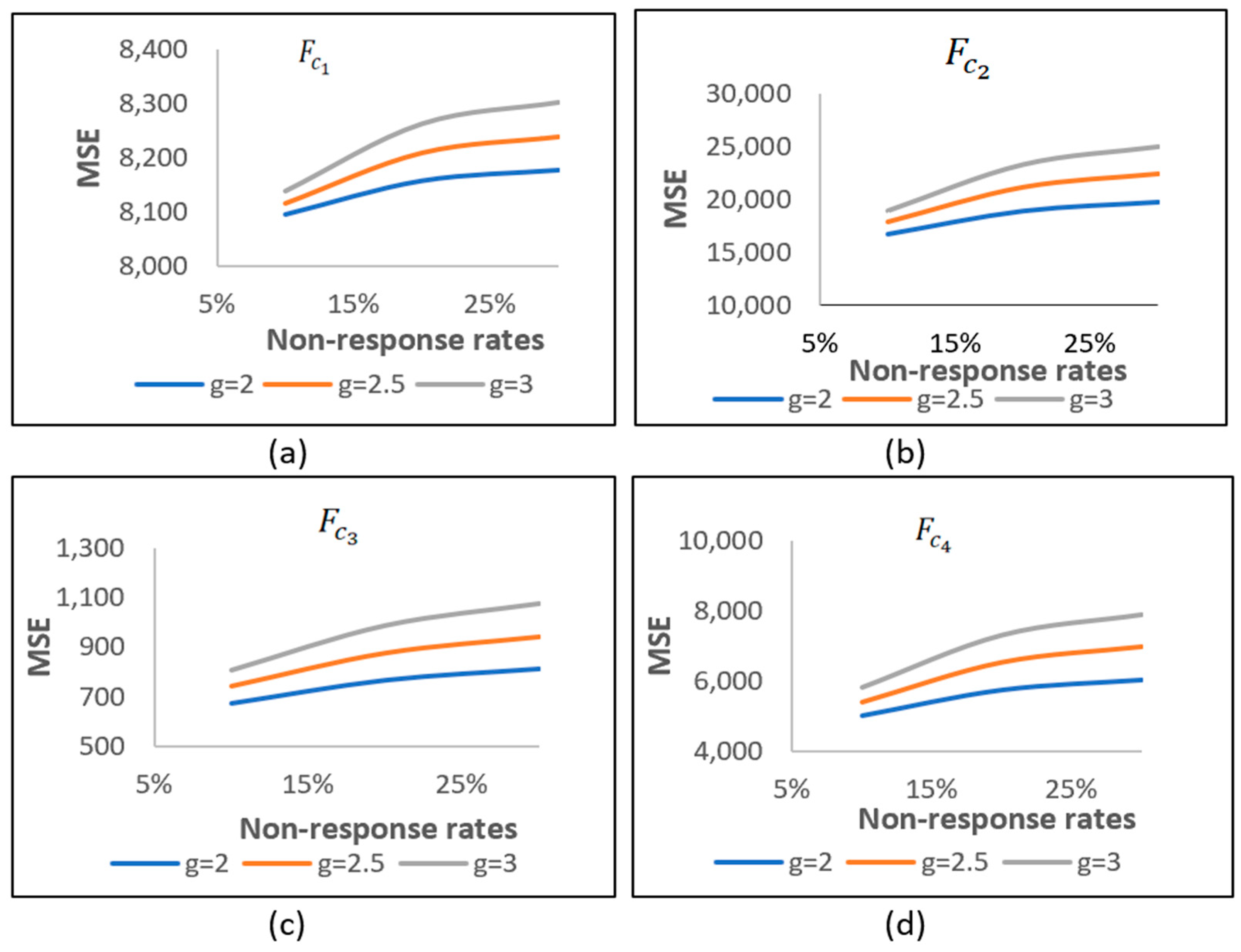
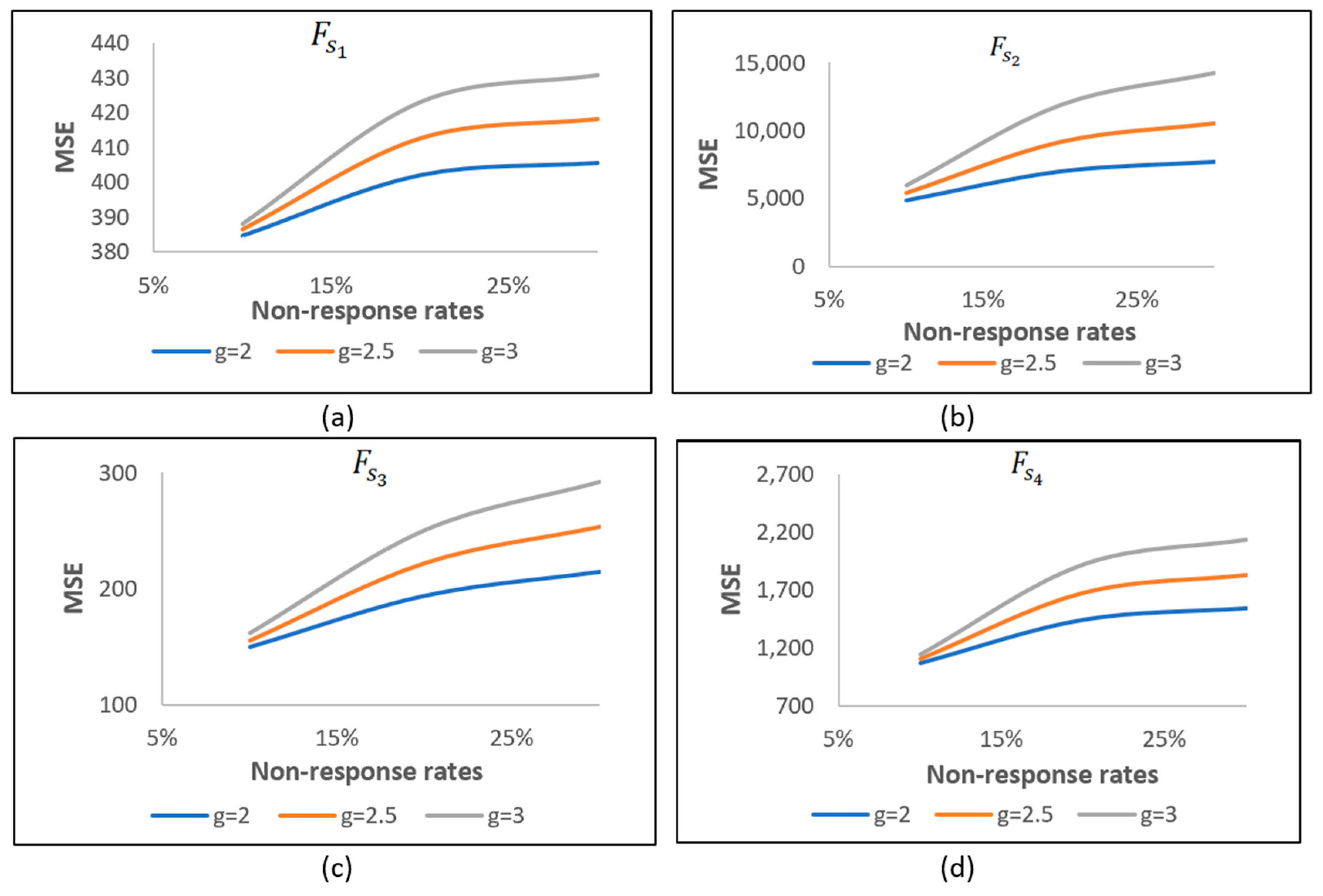
Table 1, we place a specific emphasis on case (i), where NR occurs in both the study and auxiliary variables. Table 1 clearly demonstrates that the MSE values rise in parallel with the growth in both the NR rates and the values of the constant g . In addition, we displayed this information visually in Figure 1 and Figure 2. The estimators ( F c 1 , F c 2 , F c 3 , F c 4 )   are denoted collectively as (a), (b), (c), and (d) in Figure 1. In Figure 2, the separate estimators ( F s 1 , F s 2 ,   F s 3 , F s 4 ) are labelled separately as (a), (b), (c), and (d). It is observed that the MSE values consistently increase with the NR rates.
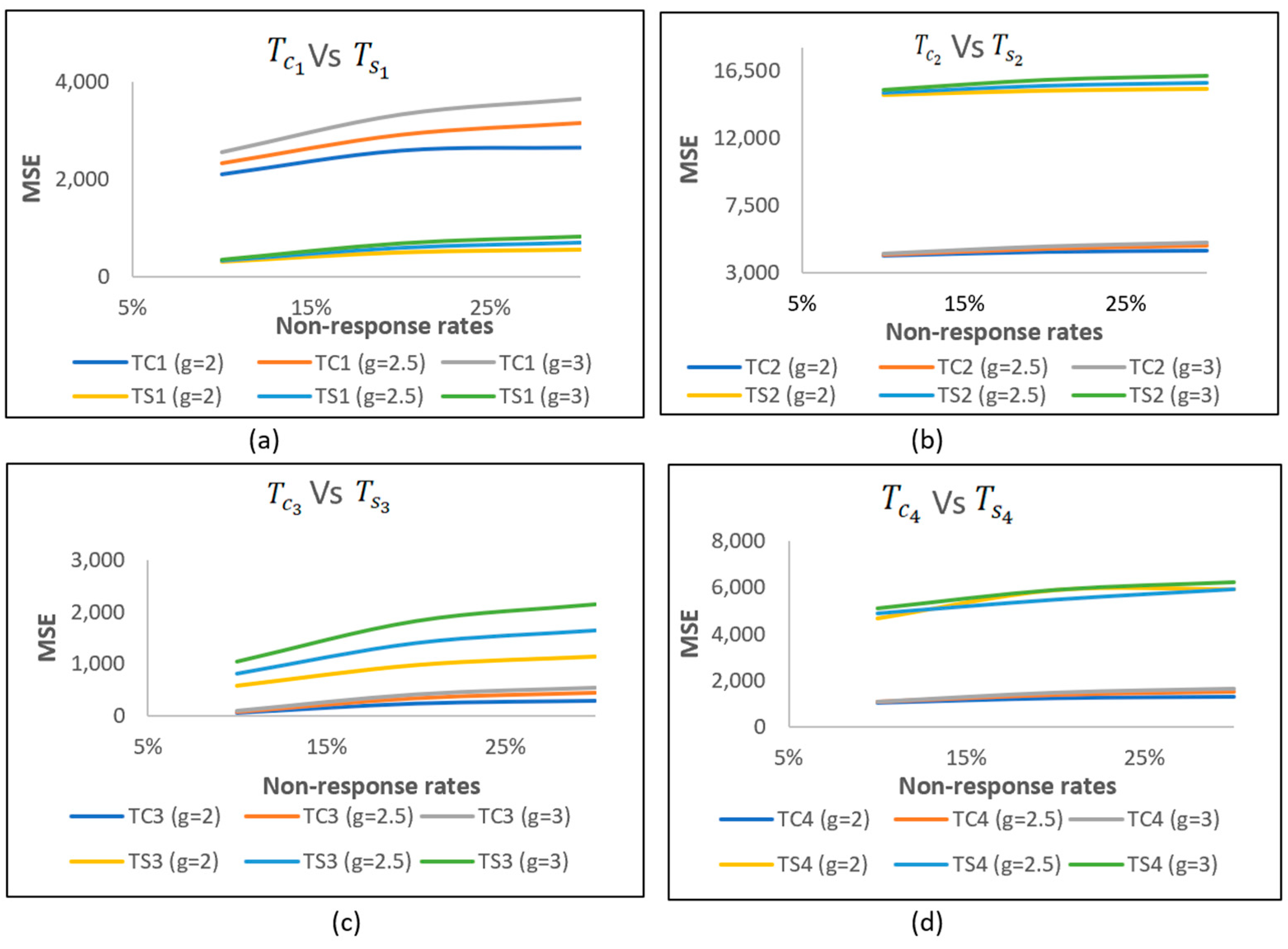
The efficiencies of combined and separate estimators were compared using the results from Table 2, focusing on case (ii), where NR occurs only in the study variable. It was observed that separate estimators generally exhibit greater efficiency than combined estimators when they are evaluated using MSE metrics. Figure 3a–d illustrate comparisons between the estimators ( T c 1 , T s 1 ) ,   ( T c 2 , T s 2 ) , ( T c 3 , T s 3 )   a n d   ( T c 4 , T s 4 ) , respectively. The observed differences in MSE values between combined and separate estimators may depend on the nature and properties of the datasets. Table 3 and Table 4 demonstrate that MSE values are higher when NR occurs in both variables compared to when it only affects the study variable. For example, with a 10% NR rate and g = 2, the MSE of F c 1 is greater than T c 1 (58.93 > 34.37), emphasising the significance of response rates in data analysis. Similarly, at g = 2.5, the MSE of F c 1 surpasses T c 1 (60.04 compared to 34.67), and at g = 3, F c 1 exceeds T c 1 (61.14 compared to 34.98).
The analysis indicates that the NR rates significantly impact the bias and MSE of the cost of living plus rent index estimation. Higher NR rates generally lead to an increased bias and MSE (presented in Table 5 and Table 6), indicating the importance of addressing NR in survey designs to ensure accurate and reliable estimates. Overall, the stratification by the cost of living index and the use of Neyman allocation provided a robust framework for sampling. The auxiliary variables (cost of living index and rent index) were effective in improving the estimation of the study variable Y . The same results are observed in the fouth population, which predicts the solar UV radiation from Table 7 and Table 8. Further investigations into specific g values and their effects on the bias and MSE could provide more insights for optimising sampling strategies in future studies. As the sample size increases, the efficiency of the proposed estimators increases as well.
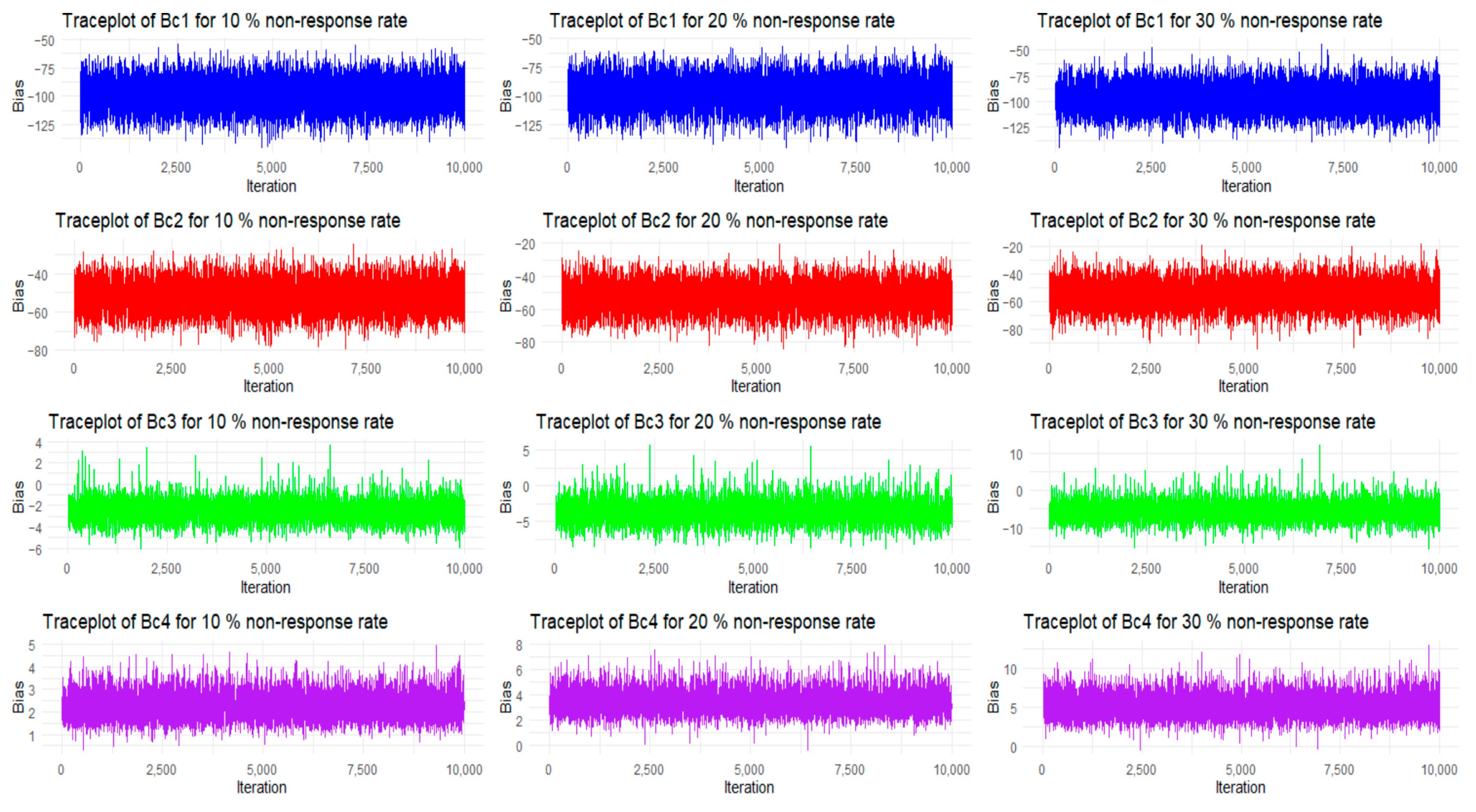
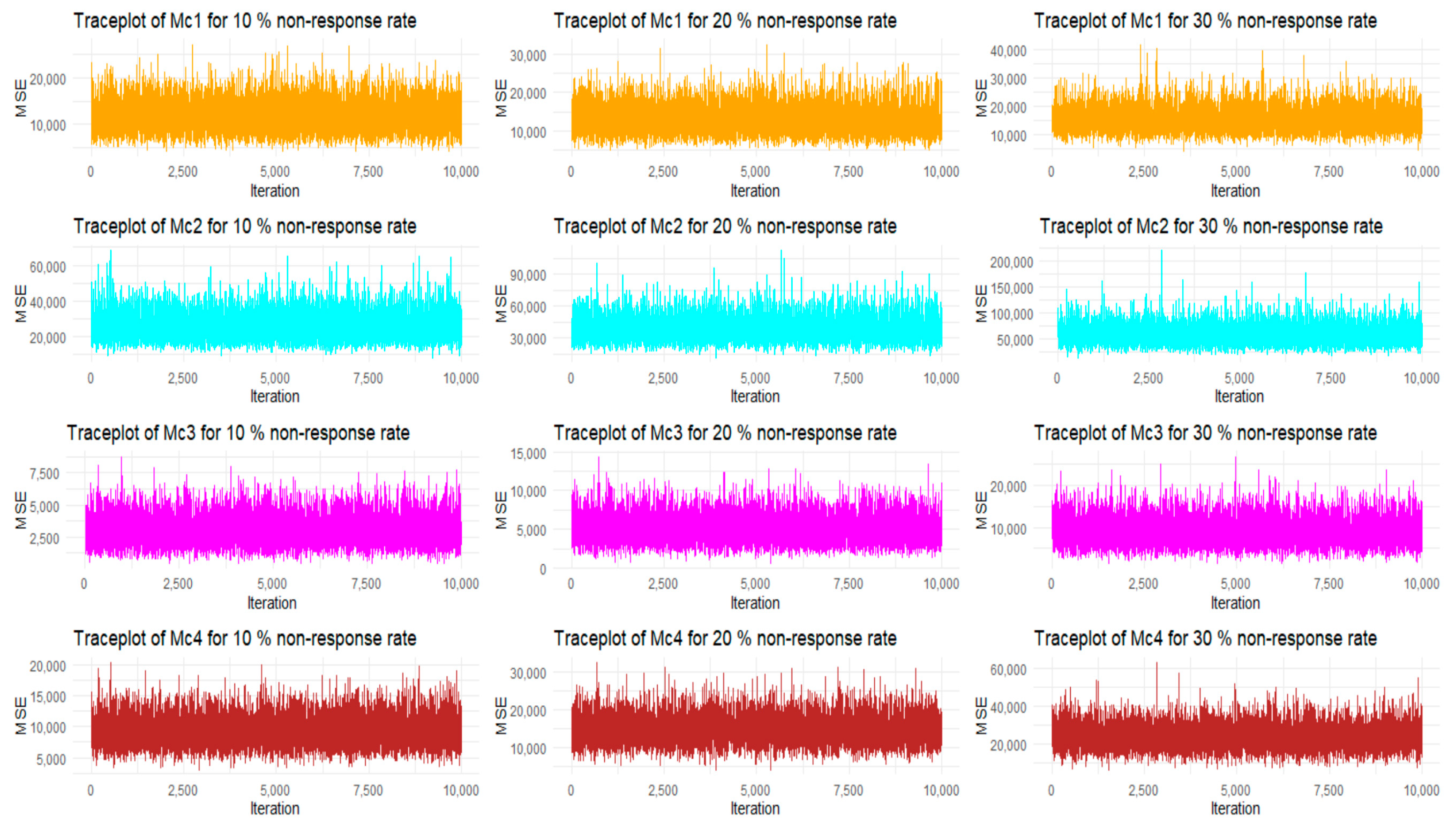
In the simulation study, we carried out 10,000 iterations to obtain the best values for the bias and MSE; we depict the bias and MSE values for each iteration in Figure 4 and Figure 5. Here, in graphs 4 and 5, we consider the combined-type estimators from Table 9, and the plots are taken for the bias and MSE values of F c 1 ,   F c 2 , F c 2 , F c 4 (in graph, bias is denoted by Bc1, Bc2, Bc3, and Bc4, and MSEs are denoted by Mc1, Mc2, Mc3, and Mc4) under 10%, 20%, 30% of NR rates.

6. Conclusions

In this study, we researched the nature of non-response (NR) in different situations and conditions under a stratified sampling scheme. We proposed combined and separate log-type families of estimators and derived their bias and MSE metric equations in the form of theorems and proofs. In addition, we conducted comparisons on several factors, which are discussed in the points below. For proving these arguments, we have utilised four real datasets and a simulation study with 10,000 iterations. The results presented in various tables clearly showed the results of the arguments and additionally, the graphs clearly represented the results.
  • The effect of varying NR rates (10% (low), 20% (medium), and 30% (high)) on MSE values was shown.
  • Evaluations were proivded of how well combined-type and separate-type estimators perform in the presence of NR.
  • The dissimilarity of MSEs of the same estimators under two NR scenarios was shown: one in which NR is present in both the study and auxiliary variables, and the other in which NR is present only in the study variable.
  • In this simulated study, we looked at different non-response rates in survey data and compared the biases and MSEs of combined and separate estimators. The performance and reliability of the estimators can be understood by methodically examining these measures across many circumstances. Survey practitioners might use the results as a reference when choosing reliable estimation methods. The results help improve the efficiency and precision of survey estimations when non-response is present.
Scope for Future Work: The study presented log-type estimators across different non-response scenarios, utilising both real datasets and simulations. Future research may investigate systematic methods for selecting tuning parameters and addressing multicollinearity in auxiliary variables. Furthermore, the integration of these estimators with conventional survey weighting methods may improve their applicability. Alternative transformations, such as Box–Cox transformations, may be utilised for the purpose of variance stabilisation. In conclusion, the comparison of log-type estimators with traditional estimators regarding the Percentage Relative Efficiency (PRE) represents a significant avenue for future research.

Author Contributions

Conceptualisation, G.R.V.T. and F.D.; methodology, F.D. and G.R.V.T.; software, G.R.V.T.; validation, G.R.V.T. and F.D.; formal analysis, G.R.V.T. and M.A.; investigation, F.D. and M.A.; resources, F.D. and G.R.V.T.; data curation, G.R.V.T.; writing—original draft preparation, G.R.V.T. and F.D.; writing—review and editing, F.D. and M.A.; visualisation, G.R.V.T. and F.D.; supervision, F.D. and M.A.; project administration, F.D. and M.A. All authors have read and agreed to the published version of the manuscript.

Funding

This work was supported by the Deanship of Scientific Research, Vice Presidency for Graduate Studies and Scientific Research, King Faisal University, Saudi Arabia [Grant No. KFU251230].

Data Availability Statement

Conflicts of Interest

The authors declare no conflicts of interest.

Appendix A

Table A1. The following error terms and their expectations were used to obtain bias and MSE when NR exists in both the study and auxiliary variables.
For Combined EstimatorsFor Separate Estimators
δ 0 s t * = y ¯ s t * Y ¯ Y ¯ , δ 1 s t * = x ¯ s t * X ¯ X ¯ and δ 2 s t * = z ¯ s t * Z ¯ Z ¯
E δ i s t * = 0 ,   i = 0,1 , 2
δ 0 h * = y ¯ h * Y ¯ Y ¯ , δ 1 h * = x ¯ h * X ¯ X ¯ and δ 2 h * = z ¯ h * Z ¯ Z ¯
E δ i h * = 0 ,   i = 0,1 , 2 .
E ( δ 0 s t * 2 ) = 1 Y ¯ 2 h = 1 L W h 2 φ h S y h 2 + φ h * S y h ( 2 ) 2 = χ y * E ( δ 1 s t * 2 ) = 1 X ¯ 2 h = 1 L W h 2 φ h S x h 2 + φ h * S x h ( 2 ) 2 = χ x * E ( δ 2 s t * 2 ) = 1 Z ¯ 2 h = 1 L W h 2 φ h S z h 2 + φ h * S z h ( 2 ) 2 = χ z * E δ 0 s t * δ 1 s t * = 1 Y ¯ X ¯ h = 1 L W h 2 φ h S y x h + φ h * S y x h ( 2 ) = χ y x * E δ 1 s t * δ 2 s t * = 1 X ¯ Z ¯ h = 1 L W h 2 φ h S x z h + φ h * S x z h ( 2 ) = χ x z * E δ 0 s t * δ 2 s t * = 1 Y ¯ Z ¯ h = 1 L W h 2 φ h S y z h 2 + φ h * S y z h 2 2 = χ y z * E ( δ 0 h * 2 ) = 1 Y ¯ h 2 φ h S y h 2 + φ h * S y h ( 2 ) 2 = ϕ y h * E ( δ 1 h * 2 ) = 1 X ¯ h 2 φ h S x h 2 + φ h * S x h ( 2 ) 2 = ϕ x h * E ( δ 2 h * 2 ) = 1 Z ¯ h 2 φ h S z h 2 + φ h * S z h ( 2 ) 2 = ϕ z h * E δ 0 h * δ 1 h * = 1 Y ¯ h X ¯ h φ h S y x h 2 + φ h * S y x h ( 2 ) 2 = ϕ y x h * E δ 1 h * δ 2 h * = 1 X ¯ h Z ¯ h φ h S x z h 2 + φ h * S x z h ( 2 ) 2 = ϕ x z h * E δ 0 h * δ 2 h * = 1 Y ¯ h Z ¯ h φ h S y z h 2 + φ h * S y z h ( 2 ) 2 = ϕ y z h *
Table A2. The following error terms and their expectations were used to obtain bias and MSE when NR exists only in the study variable.
For Combined EstimatorsFor Separate Estimators
δ y s t * = y ¯ s t * Y ¯ Y ¯ , δ x s t = x ¯ s t X ¯ X ¯ and δ z s t = z ¯ s t Z ¯ Z ¯
E ( δ y s t * ) = E δ i s t = 0 ,   i = x , z .
δ y h * = y ¯ h * Y ¯ Y ¯ , δ x h = x ¯ h X ¯ X ¯ and δ z h = z ¯ h Z ¯ Z ¯
E ( δ y h * ) = E δ i h * = 0 ,   i = x , z .
E ( δ y s t * 2 ) = 1 Y ¯ 2 h = 1 L W h 2 φ h S y h 2 + φ h * S y h ( 2 ) 2 = χ y * E ( δ x s t 2 ) = 1 X ¯ 2 h = 1 L W h 2 φ h S x h 2 = χ x E ( δ z s t 2 ) = 1 Z ¯ 2 h = 1 L W h 2 φ h S z h 2 = χ z E δ y s t * δ x s t = 1 Y ¯ X ¯ h = 1 L W h 2 φ h S y x h = χ y x E δ x s t δ z s t = 1 X ¯ Z ¯ h = 1 L W h 2 φ h S x z h = χ x z E δ y s t * δ z s t = 1 Y ¯ Z ¯ h = 1 L W h 2 φ h S y z h = χ y z E ( δ y h * 2 ) = 1 Y ¯ h 2 φ h S y h 2 + φ h * S y h 2 = ϕ y h * E ( δ x h 2 ) = 1 X ¯ h 2 φ h S x h 2 = ϕ x h E ( δ z h 2 ) = 1 Z ¯ h 2 φ h S z h 2 = ϕ z h E δ y h * δ x h = 1 Y ¯ h X ¯ h φ h S y x h = ϕ y x h E δ x h δ z h = 1 X ¯ h Z ¯ h φ h S x z h = ϕ x z h E δ y h * δ z h = 1 Y ¯ h Z ¯ h φ h S y z h = ϕ y z h
Proof of Theorem 1. 
To obtain the expressions of bias and MSE for F c 1 , we need to transform the F c 1 in terms of δ s t * ’s (by using Table A1) as follows:
F c 1 = α 1 y ¯ s t * X ¯ x ¯ s t * 1 + γ 1 l o g z ¯ s t * Z ¯ β 1 = α 1 Y ¯ ( 1 + δ 0 s t * ) ( 1 + δ 1 s t * ) 1 + γ 1 l o g ( 1 + δ 2 s t * ) β 1 (by using Table A1).
By deviating Y ¯ on both sides of the above equation, we obtain the following:
F c 1 Y ¯ = Y ¯ α 1 1 + δ 0 s t * δ 1 s t * δ 0 s t * δ 1 s t * + β 1 γ 1 ( δ 2 s t * + δ 0 s t * δ 2 s t * δ 1 s t * δ 2 s t * + 1 2 ( β 1 1 ) ( γ 1 1 ) δ 2 s t * 2 ) 1
By applying expectations on both sides of the (A1), we acquire the bias expression as follows:
B i a s ( F c 1 ) = Y ¯ α 1 1 + χ x * χ y x * + β 1 γ 1 ( χ y z * χ x z * + 1 2 ( β 1 1 ) ( γ 1 1 ) χ z * ) 1
On squaring both sides of the (A1),
F c 1 Y ¯ 2 = Y ¯ 2 1 + α 1 2 1 + δ 0 s t * 2 + 3 δ 1 s t * 2 + δ 2 s t * 2 β 1 γ 1 β 1 γ 1 + 4 δ 0 s t * δ 2 s t * δ 1 s t * δ 2 s t * 4 δ 0 s t * δ 1 s t * 2 α 1 1 + δ 1 s t * 2 δ 0 s t * δ 1 s t * + β 1 γ 1 ( δ 0 s t * δ 2 s t * δ 1 s t * δ 2 s t * + 1 2 ( β 1 1 ) ( γ 1 1 ) δ 2 s t * 2 )
by applying expectation both sides of above equation, we obtain the MSE as follows:
M S E ( F c 1 ) = Y ¯ 2 1 + α 1 2 1 + χ y * + 3 χ x * + χ z * β 1 γ 1 β 1 γ 1 + 4 χ y z * χ x z * 4 χ y x * 2 α 1 1 + χ x * χ y x * + β 1 γ 1 ( χ y z * χ x z * + 1 2 ( β 1 1 ) ( γ 1 1 ) χ z * )
Proof of Theorem 2. 
To obtain the expressions of the bias and MSE for F c 2 , we need to transform the F c 2 in terms of δ s t * ’s (by using Table 1) as follows:
F c 2 = α 2 y ¯ s t * x ¯ s t * X ¯ 1 + γ 2 l o g Z ¯ z ¯ s t * β 2 = α 2 Y ¯ ( 1 + δ 0 s t * ) ( 1 + δ 1 s t * ) 1 + γ 2 l o g ( 1 + δ 2 s t * ) 1 β 2 (by using Table A1).
By deviating Y ¯ on both sides of the above equation, we obtain the following:
F c 2 Y ¯ = Y ¯ α 2 1 + δ 0 s t * + δ 1 s t * + δ 0 s t * δ 1 s t * β 2 γ 2 ( δ 2 s t * + δ 0 s t * δ 2 s t * + δ 1 s t * δ 2 s t * 1 2 ( β 2 1 ) ( γ 2 + 1 ) δ 2 s t * 2 ) 1
By applying expectations on both sides of (A4), we acquire the bias expression as follows:
B i a s ( F c 2 ) = Y ¯ α 2 1 + χ y x * β 2 γ 2 ( χ y z * + χ x z * 1 2 ( β 2 1 ) ( γ 2 + 1 ) χ z * ) 1
On squaring both sides of (A4),
F c 2 Y ¯ 2 = Y ¯ 2 1 + α 2 2 1 + δ 0 s t * 2 + δ 1 s t * 2 + δ 2 s t * 2 β 2 γ 2 β 2 γ 2 + ( β 2 1 ) ( γ 2 + 1 ) + 4 δ 0 s t * δ 1 s t * 2 α 2 1 + δ 0 s t * δ 1 s t * β 2 γ 2 ( δ 0 s t * δ 2 s t * + δ 1 s t * δ 2 s t * 1 2 ( β 2 1 ) ( γ 2 + 1 ) δ 2 s t * 2 )
by applying expectations on both sides of the above equation, we obtain the MSE as follows:
M S E ( F c 2 ) = Y ¯ 2 1 + α 2 2 1 + χ y * + χ x * + χ z * β 2 γ 2 ( β 2 γ 2 + ( β 2 1 ) ( γ 2 + 1 ) ) + 4 χ y x * 2 α 2 1 + χ y x * β 2 γ 2 ( χ y z * + χ x z * 1 2 ( β 2 1 ) ( γ 2 + 1 ) χ z * )
Proof of Theorem 3. 
To obtain the expressions of the bias and MSE for F c 3 , we need to transform the F c 3 in terms of δ s t * ’s (by using Table 1) as follows:
F c 3 = y ¯ s t * X ¯ x ¯ s t * α 3 1 γ 3 l o g z ¯ s t * Z ¯ β 3 = Y ¯ ( 1 + δ 0 s t * ) 1 δ 1 s t * α 3 + α 3 ( α 3 + 1 ) 2 δ 1 s t * 2 1 γ 3 l o g ( 1 + δ 2 s t * ) 1 β 3 (by using Table A1).
By deviating Y ¯ on both sides of the above equation, we obtain the following:
F c 3 Y ¯ = Y ¯ δ 0 s t * α 3 δ 1 s t * β 3 γ 3 δ 2 s t * α 3 δ 0 s t * δ 1 s t * + α 3 β 3 δ 1 s t * δ 2 s t * β 3 γ 3 δ 0 s t * δ 2 s t * + α 3 ( α 3 + 1 ) 2 δ 1 s t * 2 + 1 2 β 3 γ 3 ( β 3 1 ) ( γ 3 + 1 ) δ 2 s t * 2
By applying expectations on both sides of (A7), we acquire the bias expression as follows:
B i a s F c 3 = Y ¯ α 3 χ y x * β 3 γ 3 χ y z * + α 3 χ x z * 1 2 ( β 3 1 ) ( γ 3 + 1 ) χ z * + α 3 α 3 + 1 2 χ x *
On squaring both sides of (A7),
F c 3 Y ¯ 2 = Y ¯ 2 δ 0 s t * 2 + α 3 2 δ 1 s t * 2 + β 3 2 γ 3 2 δ 2 s t * 2 2 α 3 δ 0 s t * δ 1 s t * 2 β 3 γ 3 δ 0 s t * δ 2 s t * + α 3 β 3 γ 3 δ 1 s t * δ 2 s t *
by applying expectation both sides of the above equation, we obtain the MSE as follows:
M S E ( F c 3 ) = Y ¯ 2 χ y * + α 3 2 χ x * + β 3 γ 3 ( β 3 γ 3 χ z * 2 χ y z * + 2 α 3 χ x z * ) 2 α 3 χ y x *
Proof of Theorem 4. 
To obtain the expressions of the bias and MSE for F c 4 , we need to transform the F c 4 in terms of δ s t * ’s (by using Table 1) as follows:
F c 4 = y ¯ s t * x ¯ s t * X ¯ α 4 1 γ 4 l o g Z ¯ z ¯ s t * β 4 = Y ¯ ( 1 + δ 0 s t * ) 1 + δ 1 s t * α 4 1 + β 4 γ 4 δ 2 s t * + 1 2 β 4 γ 4 ( β 4 1 ) ( γ 4 1 ) δ 2 s t * 2 (from Table A1).
By deviating Y ¯ on both sides of the above equation, we obtain the following:
F c 4 Y ¯ = Y ¯ δ 0 s t * + α 4 δ 1 s t * + β 4 γ 4 δ 2 s t * + α 4 δ 0 s t * δ 1 s t * + α 4 β 4 γ 4 δ 1 s t * δ 2 s t * + β 4 γ 4 δ 0 s t * δ 2 s t * + α 4 α 4 1 2 δ 1 s t * 2 + 1 2 β 4 γ 4 ( β 4 1 ) ( γ 4 1 ) δ 2 s t * 2
By applying expectations on both sides of (A10), we acquire the bias expression as follows:
B i a s ( F c 4 ) = Y ¯ α 4 χ y x * + β 4 γ 4 χ y z * + α 4 χ x z * + 1 2 ( β 4 1 ) ( γ 4 1 ) χ z * + α 4 ( α 4 1 ) 2 χ x *
On squaring both sides of (A10),
F c 4 Y ¯ 2 = Y ¯ 2 δ 0 s t * 2 + α 4 2 δ 1 s t * 2 + β 4 2 γ 4 2 δ 2 s t * 2 + 2 α 4 δ 0 s t * δ 1 s t * + 2 α 4 β 3 γ 3 δ 1 s t * δ 2 s t * + 2 β 4 γ 4 δ 0 s t * δ 2 s t *
by applying expectation both sides, we obtain the MSE as follows:
M S E ( F c 4 ) = Y ¯ 2 χ y * + α 4 2 χ x * + β 4 γ 4 ( β 4 γ 4 χ z * + 2 χ y z * + 2 α 4 χ x z * ) + 2 α 4 χ y x *
Table A3. Description of first population.
Stratum   ( h ) 123456
N h 127117103170205201
n h 312129383229
S y h 883.84644.921033.40810.58403.65711.72
S x h 30,486.7015,180.7727,549.6918,218.938497.7723,094.14
S z h 555.58365.46612.95458.03260.85397.05
Y ¯ h 703.74413573.17424.66267.03393.84
X ¯ h 20,804.599211.7914,309.309478.855569.9512,997.59
Z ¯ h 498.28318.33431.36311.32227.2313.71
ρ x y h 0.940.990.990.980.980.97
ρ x z h 0.940.970.980.980.970.99
ρ y z h 0.980.980.980.980.960.98
10% S y h ( 2 ) 510.57386.771872.881603.30264.19497.84
S x h ( 2 ) 9446.939198.2952,429.9934,794.94972.5612,485.10
S z h ( 2 ) 303.29278.51960.11821.46285.09287.99
ρ x y h ( 2 ) 0.99610.99750.99980.97410.98550.9324
ρ x z h ( 2 ) 0.99310.9970.99720.99120.9850.9647
ρ y z h ( 2 ) 0.99310.98710.99720.99420.9850.9647
20% S y h ( 2 ) 396.77406.151654.401333.35335.83903.91
S x h ( 2 ) 7439.168880.464574.782219.306540.438411.44
S z h ( 2 ) 274.42274.42965.42812.28188.02469.86
ρ x y h ( 2 ) 0.99540.9940.9950.97610.98790.9869
ρ x z h ( 2 ) 0.98970.98840.97890.96290.9820.9869
ρ y z h ( 2 ) 0.98980.97980.98460.99180.98180.9874
30% S y h ( 2 ) 500.26356.951 383.701 193.47289.41825.24
S x h ( 2 ) 14,017.998174.6238,379.7726,090.606511.3221,571.95
S z h ( 2 ) 284.44247.63811.21731.28180.51437.9
ρ x y h ( 2 ) 0.99630.99850.99570.97410.99030.9902
ρ x z h ( 2 ) 0.99370.98480.97710.9650.97990.9901
ρ y z h ( 2 ) 0.97390.97930.98390.99040.97990.9829
Table A4. Description of wecond population.
Stratum   ( h ) 123
N h 213426
n h 060402
S y h 12.148.345.47
S x h 76.7131.9449.55
S z h 19.4807.1013.21
Y ¯ h 37.5537.2526.39
X ¯ h 116.5793.0026.39
Z ¯ h 114.14106.50118.88
ρ x y h 0.79140.83390.7696
ρ x z h 0.98940.88200.9669
ρ y z h 0.77810.66510.5935
10% S y h ( 2 ) 08.6610.0503.95
S x h ( 2 ) 42.1413.2874.22
S z h ( 2 ) 6.255.2020.53
ρ x y h ( 2 ) 0.99970.99950.9840
ρ x z h ( 2 ) 0.97071.00000.9999
ρ y z h ( 2 ) 0.96490.99960.9819
20% S y h ( 2 ) 7.968.474.06
S x h ( 2 ) 36.5025.8259.32
S z h ( 2 ) 5.208.1816.54
ρ x y h ( 2 ) 0.99050.80260.8601
ρ x z h ( 2 ) 0.96230.98580.9956
ρ y z h ( 2 ) 0.92970.80620.8112
30% S y h ( 2 ) 12.7009.864.50
S x h ( 2 ) 37.6924.0252.26
S z h ( 2 ) 9.426.8314.54
ρ x y h ( 2 ) 0.92880.83350.8275
ρ x z h ( 2 ) 0.90620.88590.9907
ρ y z h ( 2 ) 0.96960.58770.7542

References

  1. Hansen, M.H.; Hurwitz, W.N. The Problem of Non-Response in Sample Surveys. J. Am. Stat. Assoc. 1946, 41, 517–529. [Google Scholar] [PubMed]
  2. Chaudhary, M.K.; Singh, V.K.; Shukla, R.K. Combined-Type Family of Estimators of Population Mean in Stratified Random Sampling under Non-Response. J. Reliab. Stat. Stud. 2012, 5, 133–142. [Google Scholar]
  3. Chaudhary, M.K.; Kumar, A. Estimating the Population Mean in Stratified Random Sampling Using Two-Phase Sampling in the Presence of Non-Response. World Appl. Sci. J. 2015, 33, 874–882. [Google Scholar] [CrossRef]
  4. Rachokarn, T.; Lawson, N. An Efficient Family of Estimators for the Population Mean Using Auxiliary Information in the Presence of Missing Observations. AIP Conf. Proc. 2016, 1775, 030010. [Google Scholar] [CrossRef]
  5. Rachokarn, T.; Lawson, N. An Efficient General Family of Estimators for Population Mean in the Presence of Non-Response. J. Math. Fund. Sci. 2017, 49, 283–293. [Google Scholar]
  6. Onyeka, A.C.; Ogbumuo, D.T.; Izunobi, C. Estimation of Population Mean in Stratified Random Sampling When Using Auxiliary Information in the Presence of Non-Response. Far East J. Theor. Stat. 2019, 55, 151–167. [Google Scholar] [CrossRef]
  7. Anieting, A. Two-Phase Stratified Sampling Estimator for Population Mean in the Presence of Nonresponse Using Single Auxiliary Variable. Math. J. Interdiscip. Sci. 2020, 8, 49–56. [Google Scholar] [CrossRef]
  8. Yaqub, M.; Shabbir, J.; Gupta, S.N. Estimation of Population Mean Based on Dual Use of Auxiliary Information in Non-Response. Commun. Stat. Theory Methods 2017, 46, 12130–12151. [Google Scholar] [CrossRef]
  9. Sanaullah, A.; Amin, M.N.; Hanif, M.; Koyuncu, N. Generalized Exponential-Type Estimators for Population Mean Taking Two Auxiliary Variables for Unknown Means in Stratified Sampling with Sub-Sampling the Non-Respondents. Int. J. Appl. Comput. Math. 2018, 4, 56. [Google Scholar] [CrossRef]
  10. Shahzad, U.; Hanif, M.; Koyuncu, N.; Luengo, A.G. A Family of Ratio Estimators in Stratified Random Sampling Utilizing Auxiliary Attribute Alongside the Nonresponse Issue. J. Stat. Theory Appl. 2019, 18, 12–25. [Google Scholar] [CrossRef]
  11. Singh, H.P.; Nigam, P. Efficient Method of Estimating the Finite Population Mean Based on Two Auxiliary Variables in the Presence of Non-Response under Stratified Sampling. J. Reliab. Stat. Stud. 2021, 14, 223–242. [Google Scholar] [CrossRef]
  12. Almulhim, F.A.; Aljohani, H.M.; Aldallal, R.; Mustafa, M.S.; Alsolmi, M.M.; Elshenawy, A.; Alrashidi, A. Estimation of Finite Population Mean Using Dual Auxiliary Information under Non-Response with Simple Random Sampling. Alex. Eng. J. 2024, 100, 286–299. [Google Scholar] [CrossRef]
  13. Zahid, E.; Shabbir, J. Estimation of Population Mean in the Presence of Measurement Error and Non-Response under Stratified Random Sampling. PLoS ONE 2018, 13, e0191572. [Google Scholar] [CrossRef]
  14. Nderitu, C.W.; Imboga, H.; Wanjoya, A. Estimation of Finite Population Mean Using Ratio Estimator Based on Known Median of Auxiliary Variable in the Presence of Non-Response. Am. J. Theor. Appl. Stat. 2022, 11, 75–82. [Google Scholar]
  15. Unal, C.; Kadilar, C. A New Population Mean Estimator under Non-Response Cases. J. Taibah Univ. Sci. 2022, 16, 111–119. [Google Scholar] [CrossRef]
  16. Zahid, E.; Shabbir, J.; Alamri, O.A. A Generalized Class of Estimators for Sensitive Variable in the Presence of Measurement Error and Non-Response under Stratified Random Sampling. J. King Saud Univ. Sci. 2022, 34, 101741. [Google Scholar] [CrossRef]
  17. Danish, F.; Rizvi, S.E.H.; Bouza, C. On Approximately Optimum Strata Boundaries Using Two Auxiliary Variables. Investig. Oper. 2020, 41, 445–461. [Google Scholar]
  18. Danish, F.; Rizvi, S.E.H. Approximately Optimum Strata Boundaries for Two Concomitant Stratification Variables under Proportional Allocation. Stat. Transit. New Ser. 2021, 22, 19–40. [Google Scholar]
  19. Kadılar, C.; Cıngı, H. Ratio Estimators Using Robust Regression. Hacet. J. Math. Stat. 2007, 36, 181–188. [Google Scholar]
  20. Zaman, T.; Bulut, H. Modified Regression Estimators Using Robust Regression Methods and Covariance Matrices in Stratified Random Sampling. Commun. Stat. Theory Methods 2020, 49, 3407–3420. [Google Scholar] [CrossRef]
  21. Zaman, T.; Dünder, E.; Audu, A.; Alilah, D.A.; Shahzad, U.; Hanif, M. Robust Regression-Ratio-Type Estimators of the Mean Utilizing Two Auxiliary Variables: A Simulation Study. Math. Probl. Eng. 2021, 2021, 6383927. [Google Scholar] [CrossRef]
  22. Zaman, T.; Bulut, H.; Yadav, S.K. Robust Ratio-Type Estimators for Finite Population Mean in Simple Random Sampling: A Simulation Study. Concurr. Comput. Pract. Exp. 2022, 34, e7273. [Google Scholar] [CrossRef]
  23. Zaman, T.; Bulut, H. An Efficient Family of Robust-Type Estimators for the Population Variance in Simple and Stratified Random Sampling. Commun. Stat. Theory Methods 2023, 52, 2610–2624. [Google Scholar]
  24. Kocyigit, E.G. Using past sample means in exponential ratio and regression type estimators under a simple random sampling. Soft Comput. 2025, 29, 1389–1406. [Google Scholar]
  25. Lakshmi, N.V.; Danish, F.; Alrasheedi, M. Enhanced estimation of finite population mean via power and log-transformed ratio estimators using an auxiliary variable in solar radiation data. J. Radiat. Res. Appl. Sci. 2025, 18, 101379. [Google Scholar]
  26. Singh, G.N.; Pandey, M.K.; Bandyopadhyay, A.; Meetei, M.Z.; Zaagan, A.A.; Mahnashi, A.M.; Al-Marzouki, S. Estimation of Population Mean Using Calibrated Weights in Stratified Random Successive Sampling in Presence of Incomplete Data. J. Math. 2025, 2025, 6778010. [Google Scholar]
  27. Patel, A.; Ray, B.K.; Garg, N. Generalized Calibration Estimator of Population Mean for Stratified Sampling in the Presence of Non-response. J. Indian Soc. Probab. Stat. 2025, 1–23. [Google Scholar] [CrossRef]
  28. Saleem, I.; Sanaullah, A.; Hanif, M. A Generalized Class of Estimators for Estimating Population Mean in the Presence of Non-Response. J. Stat. Theory Appl. 2018, 17, 616–626. [Google Scholar] [CrossRef]
  29. Cost of Living Index by City 2024 Mid-Year. Available online: https://www.numbeo.com/cost-of-living/rankings.jsp (accessed on 25 July 2024).
  30. Solar UV Radiation. Available online: https://www.kaggle.com/datasets/ziya07/solar-uv-radiation (accessed on 1 February 2025).
Figure 1. MSE values for different NR rates for the combined families of estimators in the case that NR occurs in both study and auxiliary variables for first population. (a) MSE of F c 1 with increase of NR rates; (b) MSE of F c 2 across different NR rates; (c) MSE of F c 3 under various NR rates; (d) MSE of F c 4 at 10%, 20% and 30% of NR.
Mathematics 13 01089 g001
Figure 2. MSE values for different NR rates for the separate families of estimators in the case that NR occurs in both study and auxiliary variables for first population. (a) MSE of F s 1 with increase of NR rates; (b) MSE of F s 2 across different NR rates; (c) MSE of F s 3 under various NR rates; (d) MSE of F s 4 at 10%, 20% and 30% of NR.
Mathematics 13 01089 g002
Figure 3. Comparing combined-type estimators and separate-type estimators when NR occurs only in study variable for first population. (a) Comparison of MSEs of T c 1 and T s 1 with increase of NR rates; (b) Comparison of MSEs of T c 2 and T s 2 with rise of NR rates; (c) Comparison of MSEs of T c 3 and T s 3 with increase of NR rates; (d) Comparison of MSEs of T c 4 and T s 4 with rise of NR rates.
Mathematics 13 01089 g003
Figure 4. Trace plots depicting the bias values for various NR rates in the simulation study.
Mathematics 13 01089 g004
Figure 5. Trace plots depicting the MSE values for various NR rates in the simulation study.
Mathematics 13 01089 g005
Table 1. NR occurs in both study and auxiliary variables: first population.
NR EstimatorCombined TypeEstimatorSeparate Type
BiasMSEBiasMSE
10% g = 2 F c 1 −86.878095.37 F s 1 −15.22384.79
F c 2 −45.1416,709.43 F s 2 −9.024862.22
F c 3 −1.87675.12 F s 3 −1.78150.12
F c 4 1.755014.22 F s 4 1.711071.23
g = 2.5 F c 1 −86.878117.63 F s 1 −15.22386.46
F c 2 −45.2517,828.86 F s 2 −9.055387.35
F c 3 −2.03740.11 F s 3 −1.83156.01
F c 4 1.895417.19 F s 4 1.751108.83
g = 3 F c 1 −86.878139.93 F s 1 −15.22388.15
F c 2 −45.3618,948.29 F s 2 −9.095989.87
F c 3 −2.19805.10 F s 3 −1.88161.91
F c 4 2.035820.15 F s 4 1.801147.57
20% g = 2 F c 1 −86.828157.32 F s 1 −15.22402.16
F c 2 −45.2918,885.82 F s 2 −9.147015.30
F c 3 −2.13765.58 F s 3 −2.33194.22
F c 4 2.015759.47 F s 4 2.271440.57
g = 2.5 F c 1 −86.798210.57 F s 1 −15.23412.61
F c 2 −45.4621,093.44 F s 2 −9.249166.30
F c 3 −2.43875.80 F s 3 −2.67222.25
F c 4 2.286535.10 F s 4 2.591675.79
g = 3 F c 1 −86.768263.86 F s 1 −15.23423.15
F c 2 −45.6423,301.07 F s 2 −9.3411,909.23
F c 3 −2.72986.01 F s 3 −2.99250.35
F c 4 2.557310.66 F s 4 2.911922.58
30% g = 2 F c 1 −86.818176.98 F s 1 −15.24405.68
F c 2 −45.3919,724.77 F s 2 −9.307730.85
F c 3 −2.25810.00 F s 3 −2.51214.92
F c 4 2.126050.79 F s 4 2.401538.53
g = 2.5 F c 1 −86.788240.13 F s 1 −15.25418.17
F c 2 −45.6322,351.87 F s 2 −9.4810,547.17
F c 3 −2.61942.43 F s 3 −2.92253.35
F c 4 2.446972.04 F s 4 2.801828.98
g = 3 F c 1 −86.748303.35 F s 1 −15.26430.92
F c 2 −45.8624,978.97 F s 2 −9.6614,276.00
F c 3 −2.961074.86 F s 3 −3.34291.89
F c 4 2.767893.30 F s 4 3.192136.34
Table 2. NR occurs only in study variable: first population.
NR EstimatorCombined TypeEstimatorSeparate Type
BiasMSEBiasMSE
10% g = 2 T c 1 0.442094.46 T s 1 0.12315.91
T c 2 −44.9314,837.70 T s 2 −8.944131.95
T c 3 −2.96586.69 T s 3 −3.1166.95
T c 4 1.474661.54 T s 4 1.621041.55
g = 2.5 T c 1 0.442321.09 T s 1 0.12332.25
T c 2 −44.9315,021.27 T s 2 −8.944193.40
T c 3 −2.96813.31 T s 3 −3.1182.19
T c 4 1.474888.17 T s 4 1.621063.17
g = 3 T c 1 0.442547.72 T s 1 0.12348.69
T c 2 −44.9315,204.84 T s 2 −8.944256.18
T c 3 −2.961039.94 T s 3 −3.1197.47
T c 4 1.475114.80 T s 4 1.621085.12
20% g = 2 T c 1 0.442587.44 T s 1 0.12493.27
T c 2 −44.9315,156.01 T s 2 −8.944402.40
T c 3 −2.96979.66 T s 3 −3.11237.45
T c 4 1.475879.66 T s 4 1.621239.94
g = 2.5 T c 1 0.442910.55 T s 1 0.12600.12
T c 2 −44.9315,498.74 T s 2 −8.944607.71
T c 3 −2.961402.78 T s 3 −3.11339.19
T c 4 1.475477.63 T s 4 1.621364.23
g = 3 T c 1 0.443333.67 T s 1 0.12708.47
T c 2 −44.9315,841.46 T s 2 −8.944820.49
T c 3 −2.961825.89 T s 3 −3.11441.96
T c 4 1.475900.75 T s 4 1.621491.43
30% g = 2 T c 1 0.442649.19 T s 1 0.12545.86
T c 2 −44.9315,287.03 T s 2 −8.944489.25
T c 3 −2.961141.42 T s 3 −3.11287.94
T c 4 1.475916.27 T s 4 1.621299.41
g = 2.5 T c 1 0.443153.18 T s 1 0.12679.90
T c 2 −44.9315,695.27 T s 2 −8.944742.26
T c 3 −2.961645.41 T s 3 −3.11415.51
T c 4 1.475920.27 T s 4 1.621455.15
g = 3 T c 1 0.443657.18 T s 1 0.12816.15
T c 2 −44.9316,103.50 T s 2 −8.945005.83
T c 3 −2.962149.40 T s 3 −3.11544.61
T c 4 1.476224.26 T s 4 1.621615.12
Table 3. NR occurs in both study and auxiliary variables: second population.
NR EstimatorCombined TypeEstimatorSeparate Type
BiasMSEBiasMSE
10% g = 2 F c 1 −6.0858.93 F s 1 7.1654.80
F c 2 −3.3083.34 F s 2 −0.35188.90
F c 3 0.204.10 F s 3 4.1816.80
F c 4 −0.0217.69 F s 4 −1.3723.86
g = 2.5 F c 1 −6.0360.04 F s 1 8.0060.23
F c 2 −3.2887.76 F s 2 −0.35207.78
F c 3 0.224.50 F s 3 4.6118.67
F c 4 −0.0318.63 F s 4 −1.5125.94
g = 3 F c 1 −5.9861.14 F s 1 8.8365.68
F c 2 −3.2892.18 F s 2 −0.35226.87
F c 3 0.244.88 F s 3 5.0420.55
F c 4 −0.0319.57 F s 4 −1.6628.04
20% g = 2 F c 1 −6.0459.63 F s 1 7.6357.70
F c 2 −3.3087.89 F s 2 −0.33203.50
F c 3 0.214.25 F s 3 4.4117.69
F c 4 −0.0218.79 F s 4 −1.4425.36
g = 2.5 F c 1 −5.9861.08 F s 1 8.7064.61
F c 2 −3.2794.58 F s 2 −0.32230.53
F c 3 0.244.71 F s 3 4.9520.02
F c 4 −0.0320.29 F s 4 −1.6228.22
g = 3 F c 1 −5.9162.53 F s 1 9.7871.54
F c 2 −3.26101.27 F s 2 −0.31258.36
F c 3 0.265.16 F s 3 5.4922.36
F c 4 −0.0321.79 F s 4 −1.8131.13
30% g = 2 F c 1 −6.0359.97 F s 1 7.9459.47
F c 2 −3.2592.77 F s 2 −0.28215.86
F c 3 0.214.75 F s 3 4.5618.22
F c 4 −0.0220.92 F s 4 −1.4827.03
g = 2.5 F c 1 −5.9661.59 F s 1 9.1767.28
F c 2 −3.23101.90 F s 2 −0.24250.03
F c 3 0.235.46 F s 3 5.1720.83
F c 4 −0.0223.49 F s 4 −1.6930.81
g = 3 F c 1 −5.8863.21 F s 1 10.3975.13
F c 2 −3.22111.03 F s 2 −0.21285.63
F c 3 0.266.17 F s 3 5.7923.46
F c 4 −0.0226.05 F s 4 −1.8934.68
Table 4. NR occurs only in study variable: second population.
NR EstimatorCombined TypeEstimatorSeparate Type
BiasMSEBiasMSE
10% g = 2 T c 1 0.6734.37 T s 1 12.09117.35
T c 2 −3.2875.00 T s 2 −0.34152.48
T c 3 0.308.90 T s 3 5.7434.92
T c 4 −0.0116.41 T s 4 −1.0719.95
g = 2.5 T c 1 0.6834.67 T s 1 12.09117.74
T c 2 −3.2875.25 T s 2 −0.34152.85
T c 3 0.309.21 T s 3 5.7435.07
T c 4 −0.0116.71 T s 4 −1.0720.06
g = 3 T c 1 0.6834.98 T s 1 12.10118.14
T c 2 −3.2875.50 T s 2 −0.34153.21
T c 3 0.309.51 T s 3 5.7435.21
T c 4 −0.0117.02 T s 4 −1.0720.16
20% g = 2 T c 1 0.6834.70 T s 1 12.10117.74
T c 2 −3.2875.27 T s 2 −0.34152.85
T c 3 0.309.24 T s 3 5.7435.10
T c 4 −0.0116.74 T s 4 −1.0720.10
g = 2.5 T c 1 0.6835.18 T s 1 12.10118.33
T c 2 −3.2875.66 T s 2 −0.34153.40
T c 3 0.309.71 T s 3 5.7435.34
T c 4 −0.0217.21 T s 4 −1.0720.28
g = 3 T c 1 0.6835.65 T s 1 12.10118.92
T c 2 −3.2876.04 T s 2 −0.34153.94
T c 3 0.3010.18 T s 3 5.7435.58
T c 4 −0.0217.69 T s 4 −1.0720.45
30% g = 2 T c 1 0.6835.90 T s 1 12.10118.93
T c 2 −3.2876.24 T s 2 −0.34153.97
T c 3 0.3010.43 T s 3 5.7435.56
T c 4 −0.0217.94 T s 4 −1.0720.43
g = 2.5 T c 1 0.6836.97 T s 1 12.10120.13
T c 2 −3.2877.11 T s 2 −0.35155.90
T c 3 0.3011.50 T s 3 5.7436.04
T c 4 −0.1219.01 T s 4 −1.0720.77
g = 3 T c 1 0.6838.04 T s 1 12.09121.33
T c 2 −3.2877.98 T s 2 −0.34156.20
T c 3 0.3012.57 T s 3 5.7436.52
T c 4 −0.0220.08 T s 4 −1.0721.12
Table 5. NR occurs in both study and auxiliary variables: third population.
NR EstimatorCombined TypeEstimatorSeparate Type
BiasMSEBiasMSE
10% g = 2 F c 1 −5.9440.60 F s 1 −0.355.04
F c 2 −3.2140.02 F s 2 −0.5812.44
F c 3 −0.090.62 F s 3 −0.180.25
F c 4 0.044.68 F s 4 0.081.12
g = 2.5 F c 1 −5.9942.53 F s 1 0.37 8.16
F c 2 −3.2954.68 F s 2 −0.6921.04
F c 3 −0.140.91 F s 3 −0.270.38
F c 4 0.066.84 F s 4 0.121.74
g = 3 F c 1 −6.1044.55 F s 1 −0.3912.20
F c 2 −3.3869.33 F s 2 −0.8031.39
F c 3 −0.181.20 F s 3 −0.360.51
F c 4 0.089.01 F s 4 0.162.41
20% g = 2 F c 1 −6.0241.45 F s 1 −0.415.01
F c 2 −3.3160.97 F s 2 −0.5319.96
F c 3 −0.141.13 F s 3 −0.170.39
F c 4 0.089.50 F s 4 0.082.02
g = 2.5 F c 1 −6.0443.98 F s 1 −0.428.36
F c 2 −3.4486.10 F s 2 −0.6036.93
F c 3 −0.211.67 F s 3 −0.240.59
F c 4 0.1114.07 F s 4 0.133.29
g = 3 F c 1 −6.0846.73 F s 1 −0.4912.94
F c 2 −3.58111.23 F s 2 −0.6658.93
F c 3 −0.282.22 F s 3 −0.320.80
F c 4 0.1518.64 F s 4 0.174.73
30% g = 2 F c 1 −6.1046.10 F s 1 −0.519.84
F c 2 −3.4788.66 F s 2 −0.6732.42
F c 3 −0.231.53 F s 3 −0.300.26
F c 4 0.1213.30 F s 4 0.121.27
g = 2.5 F c 1 −6.1251.40 F s 1 −0.5317.84
F c 2 −3.68127.63 F s 2 −0.7863.41
F c 3 −0.342.28 F s 3 −0.440.39
F c 4 0.1719.78 F s 4 0.192.14
g = 3 F c 1 −6.1657.22 F s 1 −0.5629.21
F c 2 −3.89166.60 F s 2 −0.87105.18
F c 3 −0.463.03 F s 3 −0.580.53
F c 4 0.2326.25 F s 4 0.253.18
Table 6. NR occurs only in study variable: third population.
NR EstimatorCombined TypeEstimatorSeparate Type
BiasMSEBiasMSE
10% g = 2 T c 1 0.012.54 T s 1 0.010.57
T c 2 −3.0512.35 T s 2 −0.350.83
T c 3 −0.012.14 T s 3 −0.010.54
T c 4 0.012.50 T s 4 0.010.55
g = 2.5 T c 1 0.013.62 T s 1 0.010.86
T c 2 −3.0613.22 T s 2 −0.351.09
T c 3 −0.013.21 T s 3 −0.010.83
T c 4 0.023.56 T s 4 0.010.84
g = 3 T c 1 0.014.68 T s 1 0.011.16
T c 2 −3.0714.08 T s 2 −0.361.36
T c 3 −0.014.28 T s 3 −0.011.13
T c 4 0.024.62 T s 4 0.011.15
20% g = 2 T c 1 0.015.04 T s 1 0.010.99
T c 2 −3.0814.37 T s 2 −0.351.21
T c 3 −0.014.63 T s 3 −0.010.96
T c 4 0.014.98 T s 4 0.010.98
g = 2.5 T c 1 0.017.36 T s 1 0.011.55
T c 2 −3.1016.25 T s 2 −0.361.70
T c 3 −0.016.95 T s 3 −0.011.52
T c 4 0.017.30 T s 4 0.011.54
g = 3 T c 1 0.019.67 T s 1 0.012.16
T c 2 −3.1218.12 T s 2 −0.382.22
T c 3 −0.019.26 T s 3 −0.012.12
T c 4 0.019.61 T s 4 0.012.14
30% g = 2 T c 1 0.016.79 T s 1 0.010.47
T c 2 −3.1415.80 T s 2 −0.360.76
T c 3 −0.016.38 T s 3 −0.010.44
T c 4 0.016.73 T s 4 0.010.46
g = 2.5 T c 1 0.019.98 T s 1 0.010.74
T c 2 −3.1618.37 T s 2 −0.381.01
T c 3 −0.019.57 T s 3 −0.010.71
T c 4 0.019.92 T s 4 0.010.73
g = 3 T c 1 0.0113.17 T s 1 0.011.05
T c 2 −3.1820.96 T s 2 −0.401.28
T c 3 −0.0112.76 T s 3 −0.011.02
T c 4 0.0113.11 T s 4 0.011.04
Table 7. NR occurs in both study and auxiliary variables: fourth population.
NR EstimatorCombined TypeEstimatorSeparate Type
BiasMSEBiasMSE
10% g = 2 T c 1 −108.481,178,992 T s 1 −29.1950,811,719
T c 2 −57.271,484,842 T s 2 −19.56100,199,820
T c 3 −1.841,818,392 T s 3 −2.06182,454,545
T c 4 0.631,818,310 T s 4 0.75182,426,899
g = 2.5 T c 1 −108.141,762,392 T s 1 −28.68164,367,045
T c 2 −58.512,225,550 T s 2 −20.98327,638,612
T c 3 −2.842,727,461 T s 3 −3.15600,552,403
T c 4 0.972,727,349 T s 4 1.15600,466,091
g = 3 T c 1 −107.812,345,809 T s 1 −28.17381,498,749
T c 2 −59.752,966,259 T s 2 −22.39764,503,302
T c 3 −3.843,636,530 T s 3 −4.231,405,916,555
T c 4 1.313,636,388 T s 4 1.561,405,720,104
20% g = 2 T c 1 −107.362,399,597 T s 1 −27.99408,219,322
T c 2 −60.423,035,665 T s 2 −22.68819,321,760
T c 3 −4.023,720,971 T s 3 −4.341,506,445,624
T c 4 1.403,721,078 T s 4 1.631,506,532,751
g = 2.5 T c 1 −106.463,593,439 T s 1 −26.871,350,803,822
T c 2 −63.244,551,786 T s 2 −25.602,724,260,768
T c 3 −6.115,581,330 T s 3 −6.535,024,624,948
T c 4 2.135,581,502 T s 4 2.485,024,940,823
g = 3 T c 1 −105.564,787,392 T s 1 −25.753,171,249,140
T c 2 −66.056,067,906 T s 2 −28.476,409,751,068
T c 3 −8.197,441,689 T s 3 −8.6711,840,483,518
T c 4 2.877,441,925 T s 4 3.3411,841,257,886
30% g = 2 T c 1 −106.343,680,702 T s 1 −27.071,454,097,664
T c 2 −63.294,662,315 T s 2 −25.222,934,501,665
T c 3 −6.005,718,268 T s 3 −6.295,417,089,085
T c 4 2.115,718,534 T s 4 2.395,417,712,678
g = 2.5 T c 1 −104.935,515,322 T s 1 −25.484,849,644,828
T c 2 −67.546,991,760 T s 2 −29.299,813,156,971
T c 3 −9.078,577,276 T s 3 −9.3818,150,249,032
T c 4 3.198,577,685 T s 4 3.6318,152,396,990
g = 3 T c 1 −103.527,350,202 T s 1 −23.8711,431,154,565
T c 2 −71.799,321,206 T s 2 −33.2423,154,407,818
T c 3 −12.1411,436,283 T s 3 −12.3842,867,290,974
T c 4 4.2711,436,836 T s 4 4.8942,872,433,423
Table 8. NR occurs only in study variable: fourth population.
NR EstimatorCombined TypeEstimatorSeparate Type
BiasMSEBiasMSE
10% g = 2 T c 1 0.551,818,413 T s 1 0.53182,458,420
T c 2 −54.791,475,901 T s 2 −16.6898,883,524
T c 3 0.261,818,195 T s 3 0.25182,394,274
T c 4 −0.061,818,111 T s 4 −0.06182,369,395
g = 2.5 T c 1 0.552,727,353 T s 1 0.53600,472,655
T c 2 −54.792,212,142 T s 2 −16.68323,284,693
T c 3 0.262,727,135 T s 3 0.25600,330,586
T c 4 −0.062,727,050 T s 4 −0.06600,275,485
g = 3 T c 1 0.553,636,292 T s 1 0.531,405,620,109
T c 2 −54.792,948,383 T s 2 −16.68754,286,088
T c 3 0.263,636,075 T s 3 0.251,405,369,526
T c 4 −0.063,635,990 T s 4 −0.061,405,272,341
20% g = 2 T c 1 0.553,720,887 T s 1 0.531,506,317,194
T c 2 −54.793,016,906 T s 2 −16.68807,973,503
T c 3 0.263,720,670 T s 3 0.251,506,054,376
T c 4 −0.063,720,586 T s 4 −0.051,505,953,106
g = 2.5 T c 1 0.555,581,064 T s 1 0.535,023,813,395
T c 2 −54.794,523,650 T s 2 −16.682,686,324,032
T c 3 0.265,580,847 T s 3 0.255,023,226,535
T c 4 −0.065,580,763 T s 4 −0.055.02 × 109
g = 3 T c 1 0.557,441,242 T s 1 0.5311,838,116,873
T c 2 −54.796,030,393 T s 2 −16.686,320,254,203
T c 3 0.267,441,024 T s 3 0.2511,837,077,522
T c 4 −0.067,440,940 T s 4 −0.0511,836,677,033
30% g = 2 T c 1 0.555,718,081 T s 1 0.535,416,475,894
T c 2 −54.794,634,633 T s 2 −16.682,895,122,033
T c 3 0.265,717,863 T s 3 0.255,415,857,716
T c 4 −0.065,717,779 T s 4 −0.065,415,619,323
g = 2.5 T c 1 0.558,576,855 T s 1 0.5318,147,287,412
T c 2 −54.796,950,240 T s 2 −16.689,681,054,564
T c 3 0.268,576,637 T s 3 0.2518,145,903,210
T c 4 −0.068,576,553 T s 4 −0.0618,145,369,405
g = 3 T c 1 0.5511,435,629 T s 1 0.5342,859,221,223
T c 2 −54.799,265,847 T s 2 −16.6822,842,223,498
T c 3 0.2611,435,411 T s 3 0.2542,856,766,348
T c 4 −0.0611,435,327 T s 4 −0.0642,855,819,645
Table 9. NR occurs in both study and auxiliary variables: simulation study.
NR EstimatorCombined TypeEstimatorSeparate Type
BiasMSEBiasMSE
10% g = 2 F c 1 −99.3711,462.40 F s 1 −84.1314,280.74
F c 2 −51.8621,585.80 F s 2 −61.6924,029.11
F c 3 −2.172604.27 F s 3 −9.732627.21
F c 4 1.897838.75 F s 4 10.848420.32
g = 2.5 F c 1 −99.1611,625.62 F s 1 −81.5514,580.20
F c 2 −51.9623,621.92 F s 2 −62.7726,668.49
F c 3 −2.322804.80 F s 3 −10.212863.64
F c 4 2.078587.78 F s 4 11.829277.22
g = 3 F c 1 −98.9611,788.81 F s 1 −77.5614,946.17
F c 2 −52.0625,658.04 F s 2 −63.4229,582.64
F c 3 −2.463005.32 F s 3 −10.223096.01
F c 4 2.249336.81 F s 4 12.6710,157.83
20% g = 2 F c 1 −98.6412,022.85 F s 1 −77.6314,901.42
F c 2 −52.0327,944.70 F s 2 −63.0729,421.31
F c 3 −2.743646.18 F s 3 −10.383679.22
F c 4 2.4710,582.09 F s 4 12.7711,124.93
g = 2.5 F c 1 −98.1912,490.81 F s 1 −71.1815,532.90
F c 2 −52.3033,210.38 F s 2 −64.6234,754.21
F c 3 −3.184369.76 F s 3 −10.864533.10
F c 4 2.9312,714.47 F s 4 14.5212,797.77
g = 3 F c 1 −97.7412,959.26 F s 1 −64.5613,191.06
F c 2 −52.5838,476.07 F s 2 −65.9440,223.23
F c 3 −3.625093.33 F s 3 −11.095959.75
F c 4 3.4014,846.84 F s 4 16.2514,968.57
30% g = 2 F c 1 −98.0013,207.60 F s 1 −71.3815,555.58
F c 2 −53.1637,975.07 F s 2 −64.8838,885.40
F c 3 −3.705568.62 F s 3 −10.886540.35
F c 4 3.3414,982.56 F s 4 14.5515,830.15
g = 2.5 F c 1 −97.1614,252.70 F s 1 −61.7516,418.48
F c 2 −53.9648,208.97 F s 2 −66.5349,618.41
F c 3 −4.627252.00 F s 3 −11.717298.92
F c 4 4.2419,304.24 F s 4 17.2820,287.76
g = 3 F c 1 −96.3215,302.16 F s 1 −51.8817,325.78
F c 2 −54.7658,442.88 F s 2 −68.5259,654.11
F c 3 −5.548935.37 F s 3 −12.419899.75
F c 4 5.1323,625.93 F s 4 19.9826,830.34
Table 10. NR occurs in only study variable: simulation study.
NR EstimatorCombined TypeEstimatorSeparate Type
BiasMSEBiasMSE
10% g = 2 T c 1 0.833095.51 T s 1 0.666005.05
T c 2 −51.6518,226.08 T s 2 −41.4621,084.33
T c 3 −6.892490.08 T s 3 −13.922510.18
T c 4 1.557220.33 T s 4 10.897889.09
g = 2.5 T c 1 0.833535.33 T s 1 0.626432.76
T c 2 −51.6518,582.33 T s 2 −42.6521,386.90
T c 3 −6.892929.90 T s 3 −14.902996.04
T c 4 1.557660.15 T s 4 11.088208.33
g = 3 T c 1 0.833975.15 T s 1 0.586985.89
T c 2 −51.6518,938.58 T s 2 −15.6221,569.48
T c 3 −6.893369.72 T s 3 −14.963380.67
T c 4 1.558099.97 T s 4 12.688670.03
20% g = 2 T c 1 −51.494915.58 T s 1 0.627264.21
T c 2 6.8719,613.14 T s 2 −43.4821,039.72
T c 3 1.544317.75 T s 3 −14.554398.77
T c 4 0.849033.16 T s 4 12.7910,670.03
g = 2.5 T c 1 0.816273.49 T s 1 0.547598.65
T c 2 −51.4920,713.05 T s 2 −44.9021,112.33
T c 3 −6.875675.66 T s 3 −15.305890.26
T c 4 1.5410,391.07 T s 4 13.0410,876.35
g = 3 T c 1 0.817631.39 T s 1 0.468784.58
T c 2 −51.4921,812.95 T s 2 −46.5121,563.02
T c 3 −6.877033.57 T s 3 −15.997088.90
T c 4 1.5411,748.98 T s 4 13.5011,789.07
30% g = 2 T c 1 0.828006.62 T s 1 0.609012.43
T c 2 −51.5722,184.82 T s 2 −44.0123,224.42
T c 3 −6.877398.69 T s 3 −15.767648.04
T c 4 1.5412,113.96 T s 4 13.0712,055.13
g = 2.5 T c 1 0.8210,894.01 T s 1 0.5211,028.41
T c 2 −51.5729,523.61 T s 2 −45.5331,358.95
T c 3 −6.8710,286.07 T s 3 −16.4910,762.10
T c 4 1.5415,001.34 T s 4 13.9515,856.02
g = 3 T c 1 0.8213,781.40 T s 1 0.5414,638.69
T c 2 −51.5726,862.39 T s 2 −45.0933,986.01
T c 3 −6.8713,173.46 T s 3 −16.8413,703.60
T c 4 1.5417,888.73 T s 4 14.1117,909.84
Disclaimer/Publisher’s Note: The statements, opinions and data contained in all publications are solely those of the individual author(s) and contributor(s) and not of MDPI and/or the editor(s). MDPI and/or the editor(s) disclaim responsibility for any injury to people or property resulting from any ideas, methods, instructions or products referred to in the content.

