Article

A Hybrid GAS-ATT-LSTM Architecture for Predicting Non-Stationary Financial Time Series

by
Kevin Astudillo
1,
Miguel Flores
2,3,
Mateo Soliz
4,
Guillermo Ferreira
5 and
José Varela-Aldás
1,*
1
Centro de Investigación en Mecatrónica y Sistemas Interactivos (MIST), Facultad de Ingenierías, Maestría en Big Data y Ciencia de Datos, Universidad Tecnológica Indoamérica, Ambato 180103, Ecuador
2
MODES Group, Departamento de Matemáticas, Facultad de Ciencias, Escuela Politécnica Nacional, Quito 170517, Ecuador
3
Escuela Superior de Ingeniería y Tecnología, Universidad Internacional de La Rioja, 26006 Logroño, Spain
4
Facultad de Ciencias, Escuela Politécnica Nacional, Quito 170143, Ecuador
5
Departamento de Estadística, Facultad de Ciencias Físicas y Matemáticas, Universidad de Concepción, Concepcion 4070409, Chile
*
Author to whom correspondence should be addressed.
Mathematics 2025, 13(14), 2300; https://doi.org/10.3390/math13142300
Submission received: 24 May 2025 / Revised: 4 July 2025 / Accepted: 16 July 2025 / Published: 18 July 2025

Abstract

This study proposes a hybrid approach to analyze and forecast non-stationary financial time series by combining statistical models with deep neural networks. A model is introduced that integrates three key components: the Generalized Autoregressive Score (GAS) model, which captures volatility dynamics; an attention mechanism (ATT), which identifies the most relevant features within the sequence; and a Long Short-Term Memory (LSTM) neural network, which receives the outputs of the previous modules to generate price forecasts. This architecture is referred to as GAS-ATT-LSTM. Both unidirectional and bidirectional variants were evaluated using real financial data from the Nasdaq Composite Index, Invesco QQQ Trust, ProShares UltraPro QQQ, Bitcoin, and gold and silver futures. The proposed model’s performance was compared against five benchmark architectures: LSTM Bidirectional, GARCH-LSTM Bidirectional, ATT-LSTM, GAS-LSTM, and GAS-LSTM Bidirectional, under sliding windows of 3, 5, and 7 days. The results show that GAS-ATT-LSTM, particularly in its bidirectional form, consistently outperforms the benchmark models across most assets and forecasting horizons. It stands out for its adaptability to varying volatility levels and temporal structures, achieving significant improvements in both accuracy and stability. These findings confirm the effectiveness of the proposed hybrid model as a robust tool for forecasting complex financial time series.

1. Introduction

1.1. Context

Time series analysis plays a crucial role in various fields such as finance, marketing, and climatology, enabling the identification of patterns, trend forecasting, and the detection of potential anomalies or risks. With the advancement of Data Science, these techniques have become increasingly sophisticated, broadening their scope and improving their accuracy [1]. While some time series exhibit regular behavior and can be analyzed under the assumption of stationarity, others are non-stationary, posing a greater challenge and requiring more complex transformations and models to achieve accurate forecasts [2]. In this context, it is essential to apply appropriate techniques for handling non-stationary data as the choice of model depends on both the structure of the series and the specific objective of the analysis [3].
Volatility, defined as the variance of asset returns, is a key concept in finance as it quantifies market risk. Its estimation and prediction are fundamental to investment strategies, risk management, and financial policy design [4], driving the development of both stochastic and machine learning approaches [5]. In recent years, financial time series analysis has become increasingly relevant due to the high volatility and nonlinear complexity of markets. Instruments such as stocks, futures, and indices exhibit dynamics that challenge traditional assumptions of stationarity, making them difficult to model using conventional techniques.

1.2. State of the Art

Generalized Autoregressive Conditional Heteroscedasticity (GARCH) family models have been widely used for decades to model and forecast volatility and to assess financial risk [5,6,7]. However, their performance on financial time series is often suboptimal because, like other traditional parametric approaches, they assume linear data dynamics [3]. This assumption limits their ability to capture the inherent complexity of financial markets, which typically exhibit nonlinear and non-stationary behavior [8]. In this context, GARCH models can be viewed as special cases within the broader class of Generalized Autoregressive Score (GAS) models, which have been proposed as a more robust alternative to overcome these limitations [9].
Time-varying parameters in models describing stochastic time series processes are a common phenomenon in many applied scientific disciplines [9]. However, Refs. [10,11] noted that many such models are difficult to estimate and often fail to account adequately for the shape of the conditional distribution of the data. To address this, they proposed using the score of the conditional density function as the main driver of time variation in the model parameters, allowing direct estimation via maximum likelihood. The resulting model, known as the Dynamic Conditional Score (DCS) or Generalized Autoregressive Score (GAS) model, is the approach adopted in this study.
In 1981, Cox categorized time series models with time-varying parameters into two classes: observation-driven and parameter-driven models [12]. The GAS model belongs to the former category and has the advantage of exploiting the entire conditional density structure, rather than being limited to means and higher-order moments as in other observation-driven models [10], such as Generalized Autoregressive Moving Average models [13,14] and Vector Multiplicative Error Models [15].
In 2012, Maknickiene and Maknickas enhanced prediction performance using a Long Short-Term Memory (LSTM) model, a specialized type of Recurrent Neural Network (RNN), to forecast exchange rates and foreign exchange market movements, both clear examples of financial time series [16,17,18]. LSTM networks are well suited for sequential data and function as nonlinear regressors with selective memory capabilities [3]. In recent years, various studies have successfully combined parametric models like GARCH with LSTM networks, achieving improved predictive accuracy. For example, Kim et al. proposed a hybrid approach combining LSTM with multivariate GARCH models to forecast stock index volatility [19]. Similarly, hybrid GARCH deep learning models have shown improvements in cryptocurrency price prediction, especially for erratic or short time series data [20]. Additionally, Ref. [21] highlighted the merits of hybrid strategies, showing that incorporating different GARCH variants (standard, exponential, and threshold) into LSTM architectures significantly enhances volatility forecasting for Indian commodities. This improvement is supported by evaluation metrics such as RMSE and MAE and validated through rigorous statistical tests like the Diebold–Mariano and Wilcoxon tests. Likewise, Ref. [22] demonstrated that composite models such as GARCH-GJR-LSTM consistently outperform their standalone counterparts, supporting the premise that combining econometric frameworks with the adaptive learning capacity of neural networks improves the modeling of shifting volatility and complex temporal dynamics across various forecast horizons.
The use of raw data in neural networks often obscures the individual impact of each feature on the model’s prediction [23]. To address this modeling challenge, attention mechanisms (ATT) have been introduced to assign varying importance to elements in the input sequence, enhancing both model accuracy and interpretability [24]. Initially developed for image recognition in computer vision and later applied to graph transformation tasks [25], attention mechanisms allow the model to focus on the most relevant input information. In financial applications, attention-based models such as LSTM with attention have shown notable gains in forecasting accuracy, especially for stock prices in the Chinese A-share market [26]. Similarly, Ref. [27] introduced the AT-LSTM model for financial time series forecasting, demonstrating superior performance compared to traditional models such as LSTM and ARIMA [3]. In a related effort, Ref. [28] proposed a model that incorporates segmented self-attention within an LSTM framework to mitigate performance degradation in long-term forecasts. Additionally, Zhang emphasized the robustness of LSTM networks across various forecasting tasks, including Bitcoin and gold price prediction [29].
Despite advances in both statistical and deep learning models, few studies have structuredly integrated GAS models with attention mechanisms and LSTM networks for forecasting non-stationary financial time series. This gap presents a significant research opportunity to develop hybrid models that combine the statistical rigor of traditional methods with the nonlinear learning capabilities of deep networks. From this perspective, we propose the GAS-ATT-LSTM model, which integrates the strengths of the GAS model for volatility estimation, an attention mechanism for relevance weighting, and LSTM networks for learning temporal dependencies. The GAS model captures and forecasts dynamic volatility, addressing the non-stationarity of financial data. The attention mechanism, implemented within an encoder–decoder framework, identifies the most relevant parts of the input sequence, enhancing interpretability. Finally, the LSTM component enables the model to learn complex, nonlinear, and long-term dependencies, further reinforcing forecasting accuracy.
We selected six representative financial datasets, including the Nasdaq Composite stock index; the Invesco QQQ Trust and ProShares UltraPro QQQ exchange-traded funds; and gold, silver, and Bitcoin futures prices. The datasets comprise daily observations from 1 January 2021 through 1 January 2024. Each daily entry includes six features: closing price, opening price, daily high, daily low, trading volume, and the daily exchange rate.
The structure of this paper is as follows: Section 2 describes the research materials and methods. Section 3.1 presents the results and their analysis. Finally, Section 4 provides conclusions and outlines potential future research directions.

2. Materials and Methods

2.1. Data Acquisition

In this study, financial data from six representative assets of the global markets were employed, including the Nasdaq Composite Index, the Invesco QQQ Trust and ProShares UltraPro QQQ ETFs, Bitcoin, and gold and silver futures contracts. For each asset, daily market behavior was captured through variables such as opening price, daily high and low, closing price, trading volume, and adjusted closing price.
The data were obtained from Yahoo Finance, and the analysis period varies according to the historical availability and the respective launch date of each asset. Figure 1 illustrates the historical trends of the closing prices for the selected assets.
The Nasdaq Composite (^IXIC) is one of the most widely followed stock market indices in the financial world as it provides an overview of the performance of more than 5000 leading technology and growth-oriented companies in the United States and globally. In this paper, data from 1 January 1971 to 1 January 2024 were considered.
Bitcoin (BTC-USD) is a well-known decentralized cryptocurrency whose value has exhibited extreme volatility, including sharp surges in 2017 and during the 2020–2021 period, followed by notable corrections. For this analysis, records from 17 September 2014 to 1 January 2024 were used.
The Invesco QQQ Trust (QQQ) is an exchange-traded fund (ETF) that tracks the Nasdaq-100, offering exposure to leading U.S. technology companies. Data from 3 October 1999 through 1 January 2024 were analyzed. In contrast, the ProShares UltraPro QQQ (TQQQ) is an ETF designed to deliver triple-leveraged daily returns of the Nasdaq-100 index. In this study, records from 2 November 2010 to 1 January 2024 were included.
Gold futures (GC = F) enable investors to speculate on the future price of gold, an asset traditionally regarded as a safe haven. In this study, data from 30 August 2000 through 1 January 2024 were analyzed. Hereafter, this asset will be referred to as GOLD. Similarly, silver futures (SI = F) allow speculation on the future price of silver. Beyond its role as an investment asset, silver has diverse industrial applications that influence its demand and pricing. For this analysis, data from 30 August 2000 through 1 January 2024 were considered. Hereafter, this asset will be identified as SILVER.

2.2. GAS Model

The Generalized Autoregressive Score (GAS) model is a modern statistical framework designed to model dynamic processes in time series, particularly those exhibiting heteroscedasticity and nonlinearity, common characteristics in financial return data. In the context of volatility forecasting, the GAS model is especially valuable because it adjusts its parameters based on observed changes in the data, enabling an accurate and adaptive representation of volatility.
The GAS model updates the parameters of the time series process dynamically using the score of the log-likelihood function. This approach enables the model to efficiently capture structural changes in the data over time.
According to [30], the model is specified by establishing y t R N , an N-dimentional random vector at time t, with a conditional distribution:
y t | y 1 : t 1 p ( y t ; θ t ) ,
where y 1 t 1 ( y 1 T , , y t 1 T ) T contains the past values of y t up to time t 1 , and θ T Θ R J is a vector of time-varying parameters that fully characterize the distribution p ( · ) and depend solely on y 1 : t 1 and a fixed set of additional parameters ξ . That is, θ t θ ( y 1 : t 1 , ξ ) for all t.
The evolution of the parameter vector θ t , which varies over time, is the main feature of the GAS model and is driven by the score of the conditional distribution defined in (1), with the following incorporated autoregressive component:
θ t + 1 = κ + A s t + B θ t ,
where κ , A, and B are coefficient matrices with appropriate dimensions collected in ξ , and s t is a vector proportional to the score of (1), defined as follows:
s t = S t ( θ t ) t ( y t , θ t ) .
Note that the matrix S t , of dimension J × J , is a positive definite scaling matrix known at time t, and
t ( y t , θ t ) = log p ( y t ; θ t ) θ t
is the score of (1) evaluated at θ t [10].
In this study, the GAS model was employed to model the volatility of the closing price returns of the selected financial assets between 2021 and 2024. The resulting volatility estimates were incorporated as input features in the forecasting models. By relying on conditional heteroskedasticity, the GAS model captures the dynamic variability of volatility and effectively adapts to evolving market conditions [31,32].
Further methodological developments related to the GAS model have been explored in [33], where the authors propose a comprehensive framework for volatility estimation supported by simulation-based evidence. Their findings demonstrate that the GAS model exhibits strong statistical properties and, under a variety of conditions, performs on par with or outperforms traditional GARCH-type models. These results further support the model’s suitability for volatility forecasting, particularly when paired with appropriately specified error distributions.

2.3. Volatility

Volatility is a fundamental concept in financial time series analysis because it quantifies the conditional variability of returns and reflects the risk linked to market fluctuations. Accurately modeling volatility is essential to capture nonlinear dynamics, regime shifts, and extreme events, common features of financial markets. Its integration into predictive models enhances both forecasting accuracy and robustness under uncertain conditions.
In this study, volatility is modeled as the conditional standard deviation over time of logarithmic returns using a GAS(1,1) model [10], which dynamically updates the parameters of the conditional distribution based on the score of the likelihood function.
For each financial asset included in the analysis, logarithmic returns of the closing prices were computed. The logarithmic returns r t are defined as
r t = ln P t P t 1 × 100
where r t is the logarithmic return at time t, and P t and P t 1 are the closing prices at times t and t 1 , respectively.
It is assumed that the logarithmic returns r t follow a Student’s t-distribution with zero mean and conditional variance σ t 2 :
r t t ν ( 0 , σ t 2 )
where ν > 2 represents the degrees of freedom. This specification allows for capturing heavy tails and makes the model more robust to extreme values.
The evolution of volatility is described by the following dynamic equation:
f t + 1 = ω + A s t + B f t ,
where f t = log ( σ t 2 ) is the log-conditional variance, ω , A and B are model parameters, and s t is the scaled score, defined as the derivative of the log-likelihood with respect to f t . From this relationship, the conditional volatility is recovered as
σ t = exp f t 2
Thus, the value of σ t obtained from the model represents the conditional standard deviation of returns, i.e., the expected dynamic volatility of the financial asset at time t. Since it is based on logarithmic returns, this measure is dimensionless and expressed in unitless terms.

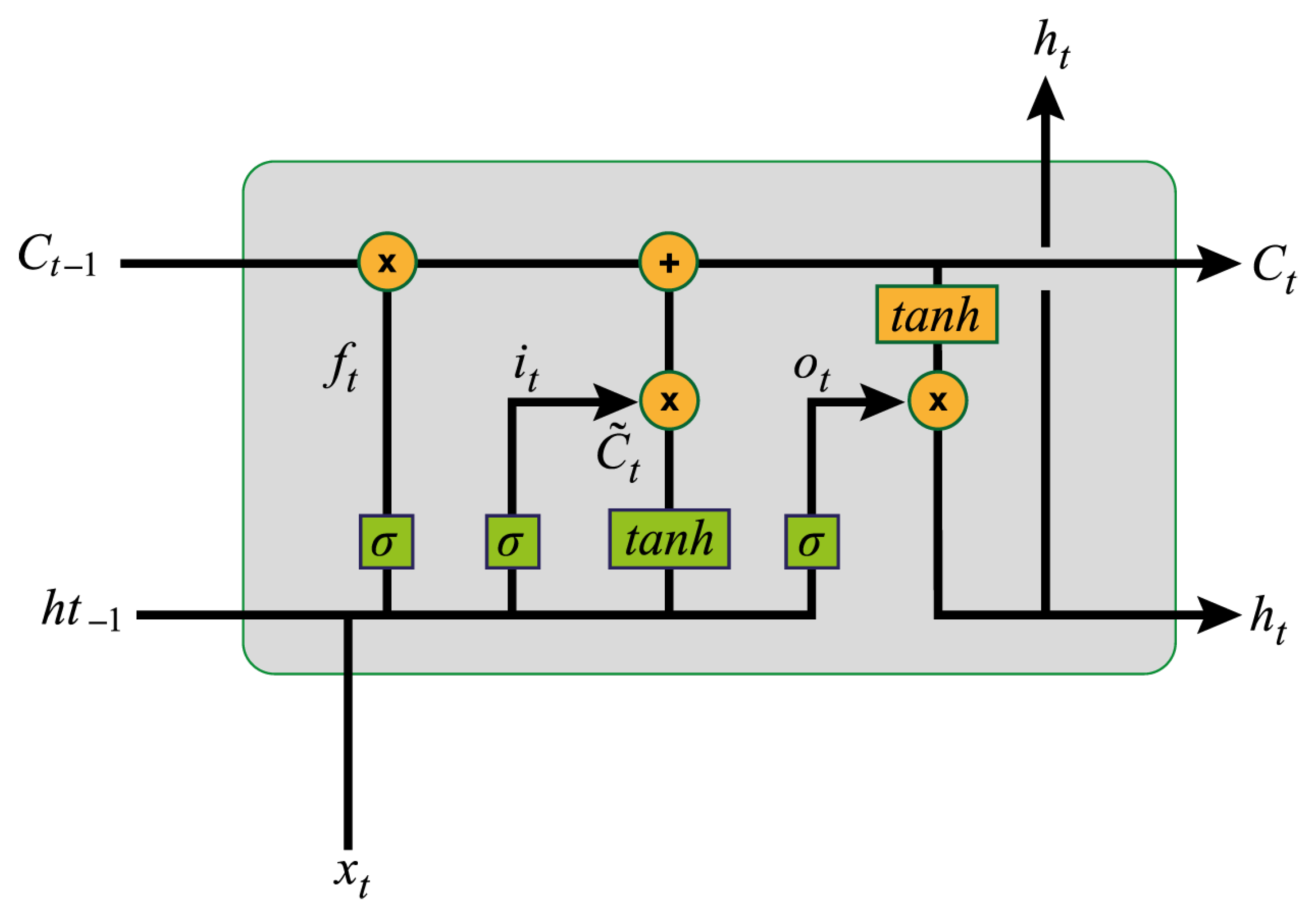
2.4. Long Short-Term Memory (LSTM)

The LSTM network, introduced by Hochreiter and Schmidhuber in 1997, is a specialized type of Recurrent Neural Network (RNN) designed to address the vanishing gradient problem [34]. While it retains the general structure of traditional RNNs, it replaces standard neurons with memory cells.
Each memory block contains three essential gates, input ( i t ) , output ( o t ) , and forget ( f t ) , which regulate the flow of information by determining what to retain and what to discard during each update of the cell state. Figure 2 illustrates the architecture of an LSTM block.
In the LSTM model, at each time step t, the input vector x t R d is processed through three main gates: input, forget, and output. These are defined, respectively, as
i t = σ ( W i x t + U i h t 1 + b i ) , f t = σ ( W f x t + U f h t 1 + b f ) , o t = σ ( W o x t + U o h t 1 + b o )
The candidate memory content is computed as
c t ˜ = tanh ( W c x t + U c h t 1 + b c )
Then, the cell state is updated using the following expression:
c t = f t c t 1 + i t c t ˜
and the hidden state is given by
h t = o t tanh ( c t )
Here, σ denotes the sigmoid activation function and tanh represents the hyperbolic tangent. The vectors b are bias terms, and W and U are learnable weight matrices. The initial states are set to c o = 0 y h o = 0 [35].

2.5. Attention Mechanism (ATT)

In financial time series forecasting, it is crucial to identify and emphasize the most relevant features while filtering out non-essential information, enabling the development of more accurate and robust predictive models that support decision-making processes [3]. Attention mechanisms enhance this process by directing the model’s focus toward the most significant segments of historical data particularly valuable when handling long-term dependencies or complex patterns.
Traditional encoder–decoder architectures like LSTM [36] compress the entire input sequence into a single fixed-length context vector, which the decoder then uses to generate predictions. However, this method often struggles with long sequences as the context vector may not retain all necessary information. Attention mechanisms overcome this limitation by enabling the decoder to dynamically access different parts of the input sequence during each step of output generation.
Additive Attention, also known as Bahdanau Attention, is a type of attention mechanism that was introduced in 2015 by Dzmitry Bahdanau in his work on machine translation with neural networks [24]. This approach enables the model to adaptively concentrate on the most pertinent segments of the input at each stage of the output generation process. It introduces a layer that computes a score ( α i j ) between the hidden state of the decoder ( s i ) and the outputs of the encoder ( h j ) to determine how much the model should focus on each part of the input sequence when generating a specific output:
α i j = v T tanh ( W t [ s i ; h j ] ) ,
where v and W are learned attention parameters, and tanh is the nonlinear activation function.
Building on the methodology proposed by [3], we implement an attention-based framework to enhance the representation of input time series for financial forecasting tasks. Let the input sequence be defined as
X t = ( x t 1 , x t 2 , , x t n ) R m ,
where n denotes the sequence length and m the dimensionality of each time step. The attention score for the k-th input at time t is computed as
α t k = v T tanh ( W x t k ) ,
yielding a score vector α t R n , where each element reflects the relevance of the corresponding input component. These scores are then normalized via the softmax function to derive attention weights β t k :
β t k = softmax ( α t k ) = exp ( α t k ) i = 1 n exp ( α t k ) ,
which quantify the relative contribution of each input feature. The final attention-enhanced representation at time t, denoted by Z t , is obtained through the weighted aggregation of the input sequence:
Z t = ( β t 1 x t 1 , β t 2 x t 2 , , β t n x t n ) T .
By using the attention weights to derive Z t , we can efficiently extract sequences of crucial input features and discard irrelevant ones. Therefore, it is expected that replacing the input of the LSTM model with Z t will result in better prediction accuracy [3].

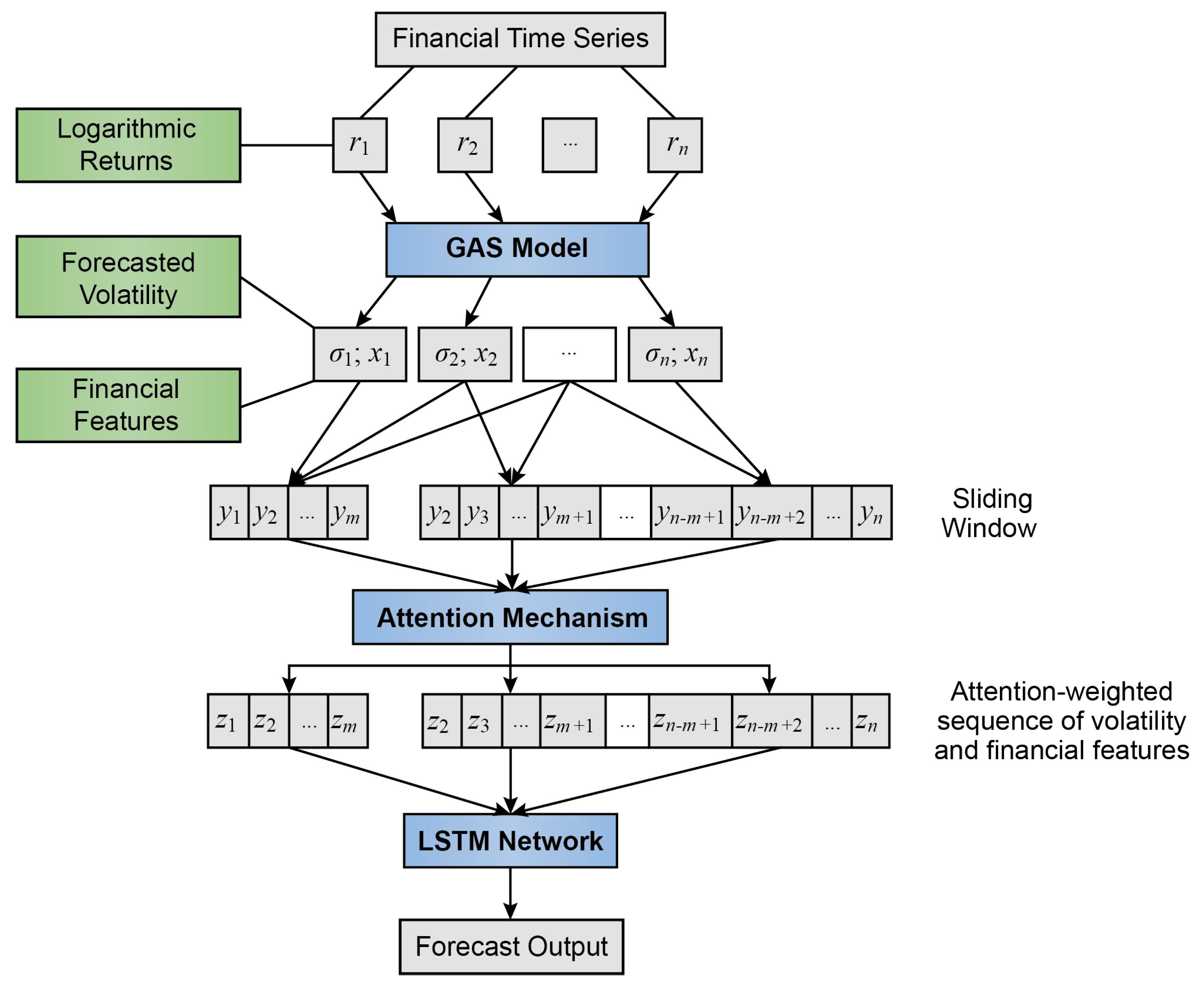
2.6. Hybrid GAS-ATT-LSTM Model

Based on the methodology proposed by [3], this article presents the GAS-ATT-LSTM model, illustrated in the architecture of Figure 3. This hybrid model integrates the GAS framework with the memory capabilities of LSTM and an attention mechanism to identify key points within a time series sequence. At each time step, the GAS model leverages the entire historical dataset and the logarithmic returns of closing prices to forecast the next-day volatility of each financial asset. This projected volatility is incorporated into the original dataset and shifted one day forward. Thus, for any given day t, the input data comprise both the original features and the volatility forecast for day t + 1 .
By integrating the volatility predictions generated by the GAS model, the architecture introduces key information related to risk levels. These forecasts are concatenated with the original financial market variables and organized into a sliding window structure, allowing the model to capture the temporal dynamics of the time series through fixed-length sequential segments.
On top of this temporal representation, a feature-level attention mechanism is applied, based on the additive attention described in Section 2.5 and the feature selection strategy outlined in [3]. Unlike conventional attention mechanisms that operate along the temporal dimension, this implementation assesses, at each time step, the relative importance of each input feature within the vector. A trainable transformation is used to generate attention scores, which are then normalized using a softmax function to produce attention weights. These weights dynamically emphasize informative features and suppress less relevant ones, yielding a refined input representation for the subsequent layers of the model.
Finally, the sequence of attention-weighted input vectors is processed by two variants of the LSTM architecture: unidirectional and bidirectional. In both cases, each point in the sequence is fed into a memory cell designed to capture nonlinear temporal dependencies at both short and long horizons, using sliding windows of 3, 5, and 7 days. This approach enhances the model’s ability to retain relevant information and improves its capacity to interpret the complex dynamics inherent in financial time series.

2.7. Data Processing

To ensure proper convergence of the neural network models and address issues arising from heterogeneous variable scales, a preprocessing procedure involving scaling and standardization was applied. The data were divided into two sets: one containing the predictor variables (Open, High, Low, Volume, and Return for each financial asset) and the other containing the target variable, corresponding to the daily closing price (Close).
The target variable was normalized using the Min–Max scaling method from the scikit-learn library, rescaling its values to the [ 0 , 1 ] interval according to the following formula:
Y s c a l e d = Y Y m i n Y m a x Y m i n
where Y is the original value, and Y m i n and Y m a x denote the minimum and maximum of the series, respectively.
The predictor variables were standardized to ensure zero mean and unit variance, allowing all features to contribute equally during model training and preventing those with larger magnitudes from disproportionately influencing parameter updates. Standardization was performed using the following expression:
X s t a n d a r i z e d = X μ σ
where X is the original feature value, μ is the mean, and σ is the standard deviation of the respective variable.

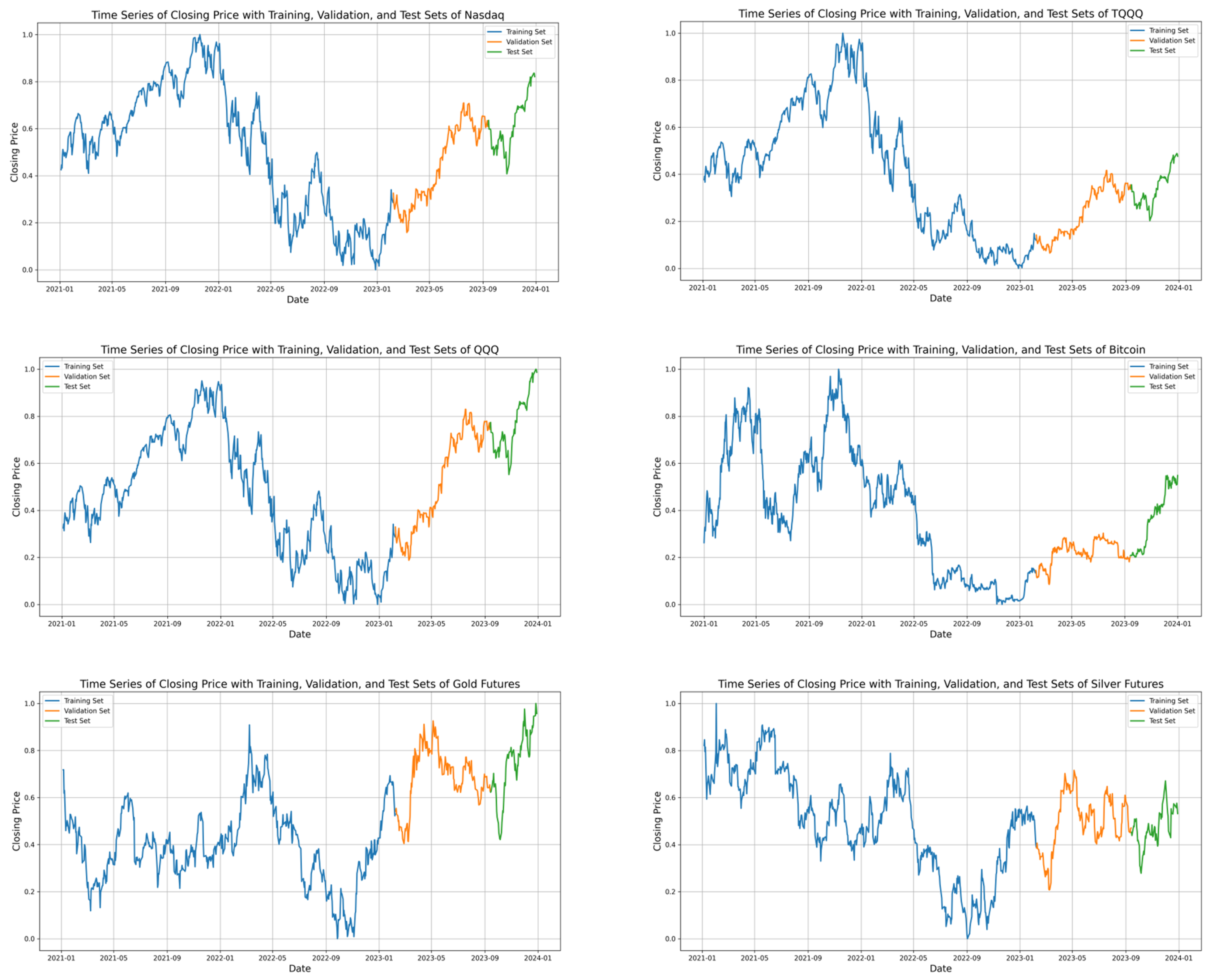
2.8. Data Partitioning

The transformed data were integrated into a single normalized dataset compatible with the input requirements of deep learning models. This dataset was chronologically divided into three subsets: 70% for training, 20% for validation, and 10% for testing, thereby streamlining the modeling process.
Each of the datasets used in the study consists of 753 observations for partitioning, except for the Bitcoin dataset, which contains 1096 observations. This difference is due to the continuous nature of the cryptocurrency market, which operates seven days a week, including weekends and holidays, unlike the traditional stock market, which records activity only on business days. The temporal ranges and the distribution of observations across each phase for the financial series are summarized in Table 1. For the other hand, Figure 4 illustrates the temporal segmentation of each financial series.

2.9. Experimental Setting

The proposed architecture, GAS-ATT-LSTM Bidirectional, incorporates an attention mechanism applied before the recurrent layers. This attention module assigns dynamic weights to each time step using a trainable matrix and vector, normalized through the softmax function. The resulting weighted sequence is then processed by a bidirectional LSTM layer with 256 units, followed by a 30% dropout layer. Subsequently, a second LSTM layer with 128 units is applied, incorporating L2 regularization and followed by a 20% dropout. The final output is generated by a dense layer with a single unit.
To ensure a fair comparison across models and to isolate the effects of architectural differences, the same set of hyperparameters was used for all LSTM-based architectures: LSTM Bidirectional, GARCH-LSTM Bidirectional, ATT-LSTM, GAS-LSTM, GAS-LSTM Bidirectional, GAS-ATT-LSTM, and GAS-ATT-LSTM Bidirectional. Each model employs two LSTM layers with 256 and 128 units, respectively, interleaved with dropout layers of 30% and 20% and ending with a dense output layer. All models were trained for 100 epochs with a batch size of 64, using the Adam optimizer, along with early stopping and learning rate reduction strategies based on validation loss.
This standardized configuration ensures that observed performance differences are solely due to architectural variations such as attention mechanisms, GARCH dynamics, or GAS components rather than differences in the training setup. The chosen hyperparameters align with common practices in financial time series modeling using LSTM, where intermediate layer sizes and dropout rates are used to balance model complexity and generalization. The two-layer recurrent structure is also standard for capturing multi-scale temporal dependencies.
The different models evaluated in the present study are as follows: LSTM Bidirectional, GARCH-LSTM Bidirectional, ATT-LSTM, GAS-LSTM, GAS-LSTM Bidirectional, GAS-ATT-LSTM, and GAS-ATT-LSTM Bidirectional.

2.10. Evaluation Metrics

In this study, the Mean Absolute Error (MAE), Root Mean Squared Error (RMSE), and the Mean Absolute Percentage Error (MAPE) are employed to evaluate the accuracy of forecasting models applied to financial time series. These metrics quantify the discrepancy between the predicted values y i ˜ and the actual observed values y i from different perspectives.
The Mean Absolute Error (MAE) is defined as
MAE = 1 N i = 1 N | y i y i ˜ |
and measures the average magnitude of the errors without considering their direction.
The Root Mean Squared Error (RMSE) is given by
RMSE = 1 N i = 1 N ( y i y i ˜ ) 2
and penalizes larger errors more severely, offering a more sensitive measure of prediction accuracy.
The Mean Absolute Percentage Error (MAPE) is calculated as
MAPE ( % ) = 1 N i = 1 N y i y i ˜ y i × 100
and expresses the average prediction error as a percentage of the actual values.

3. Results and Discussion

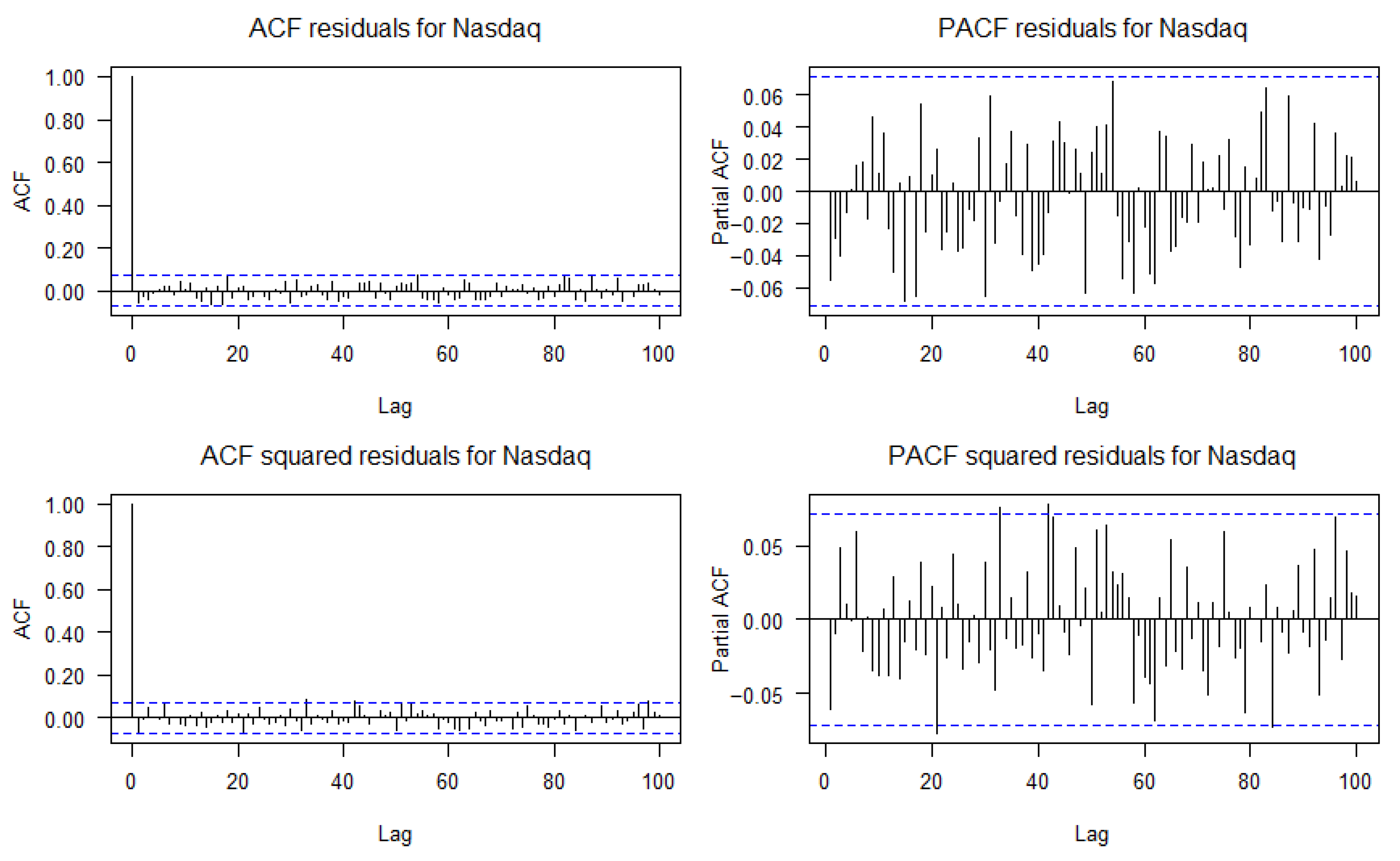
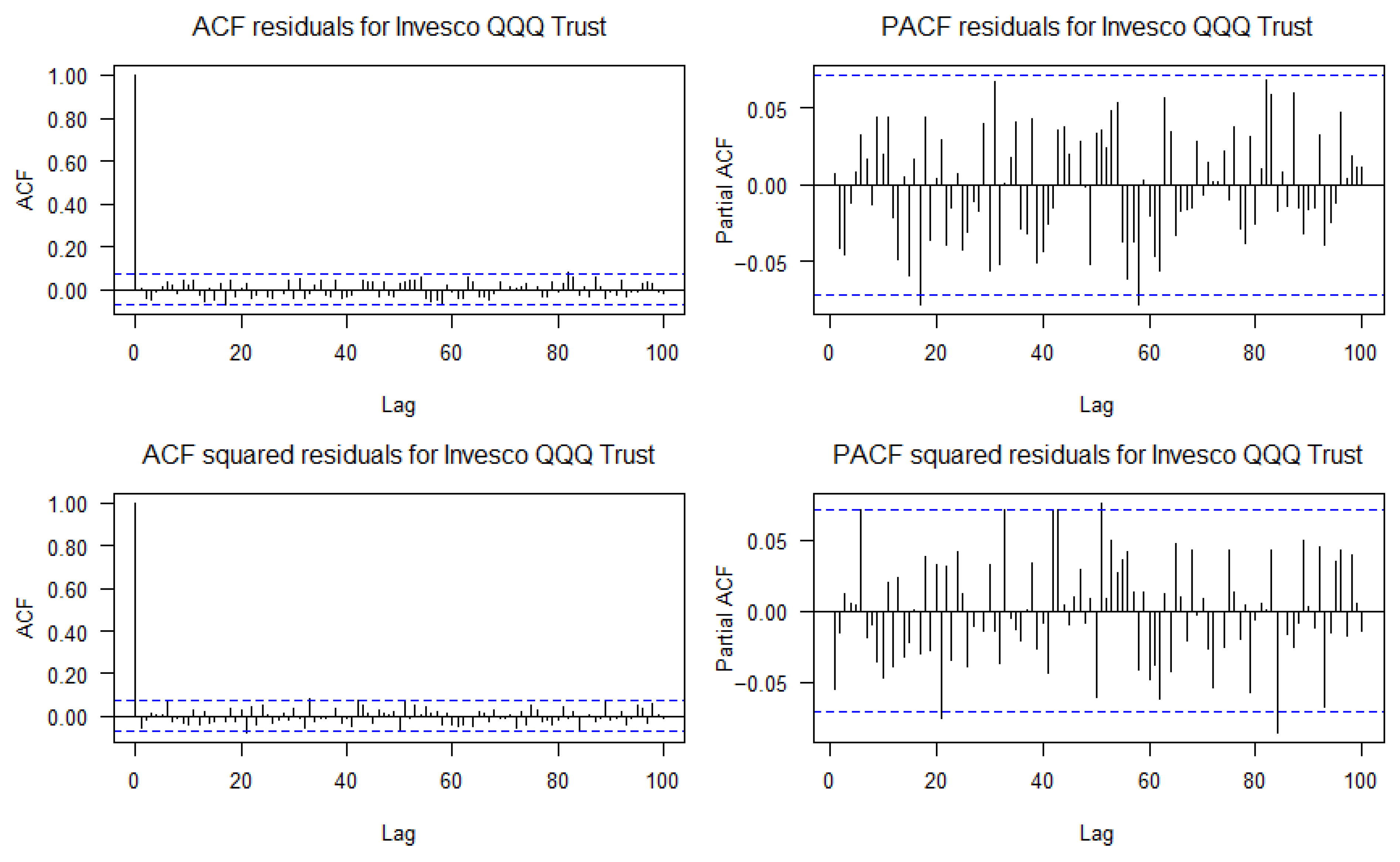
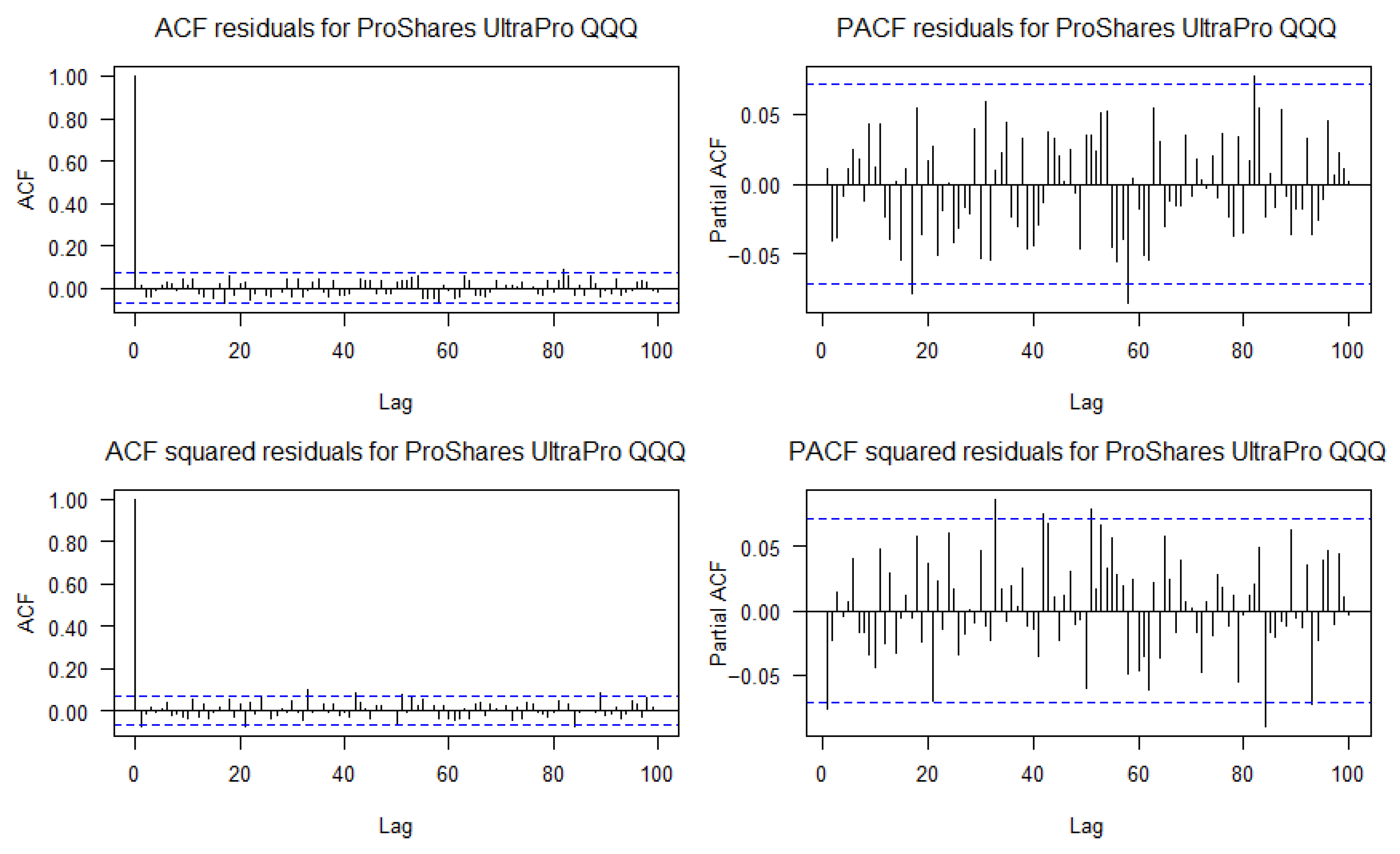
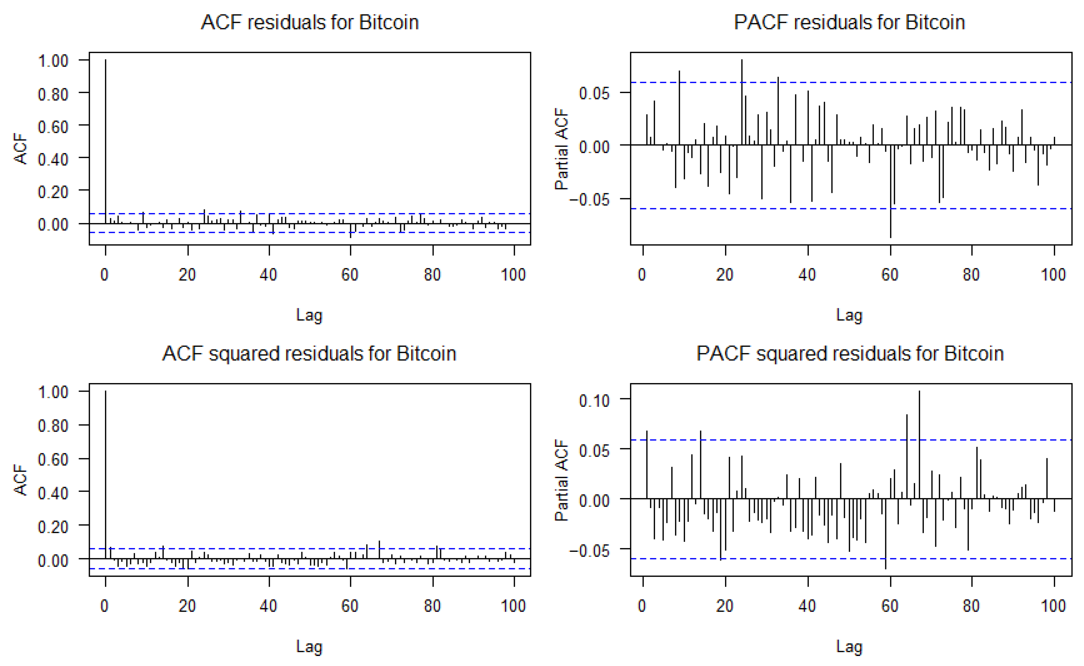
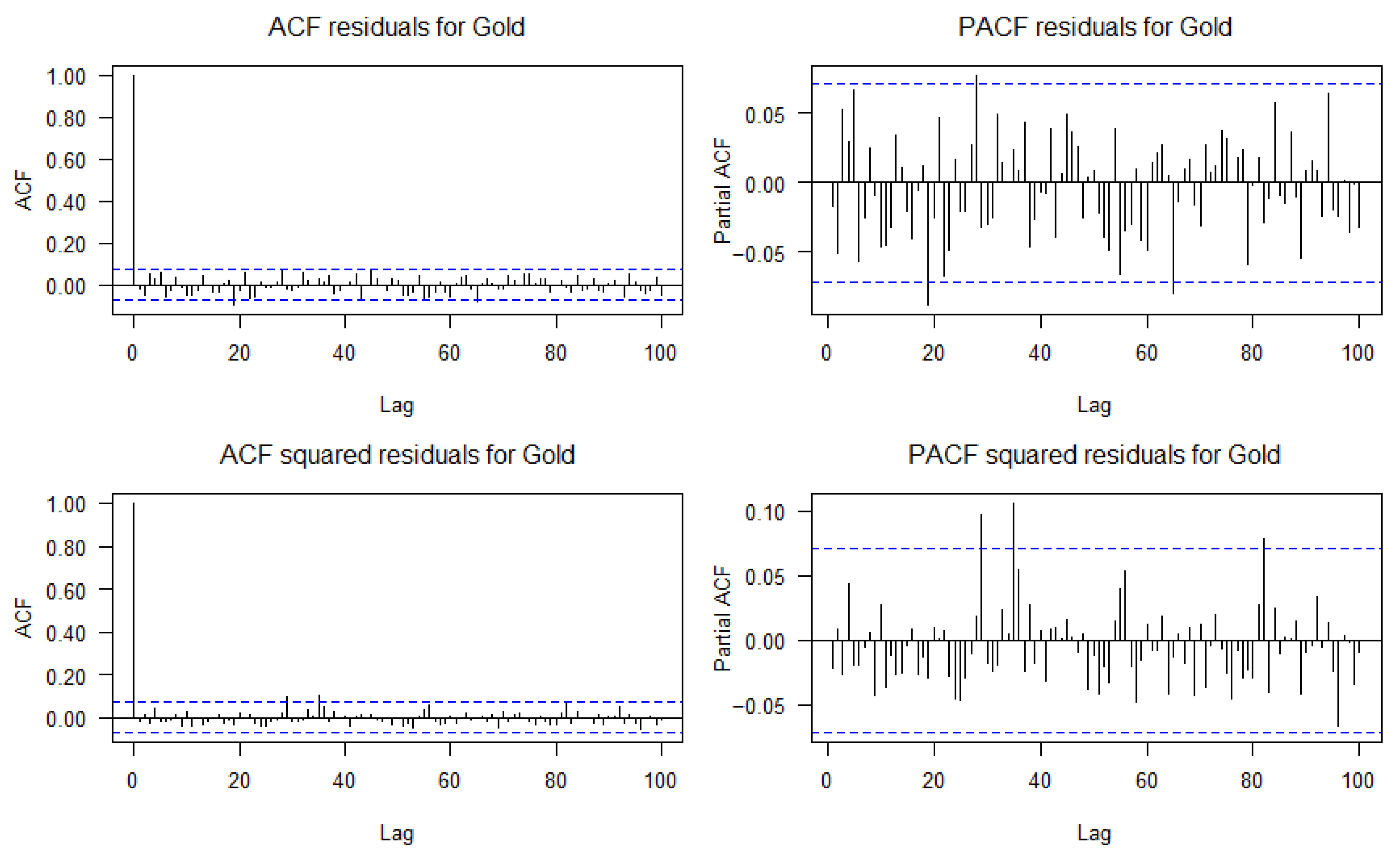
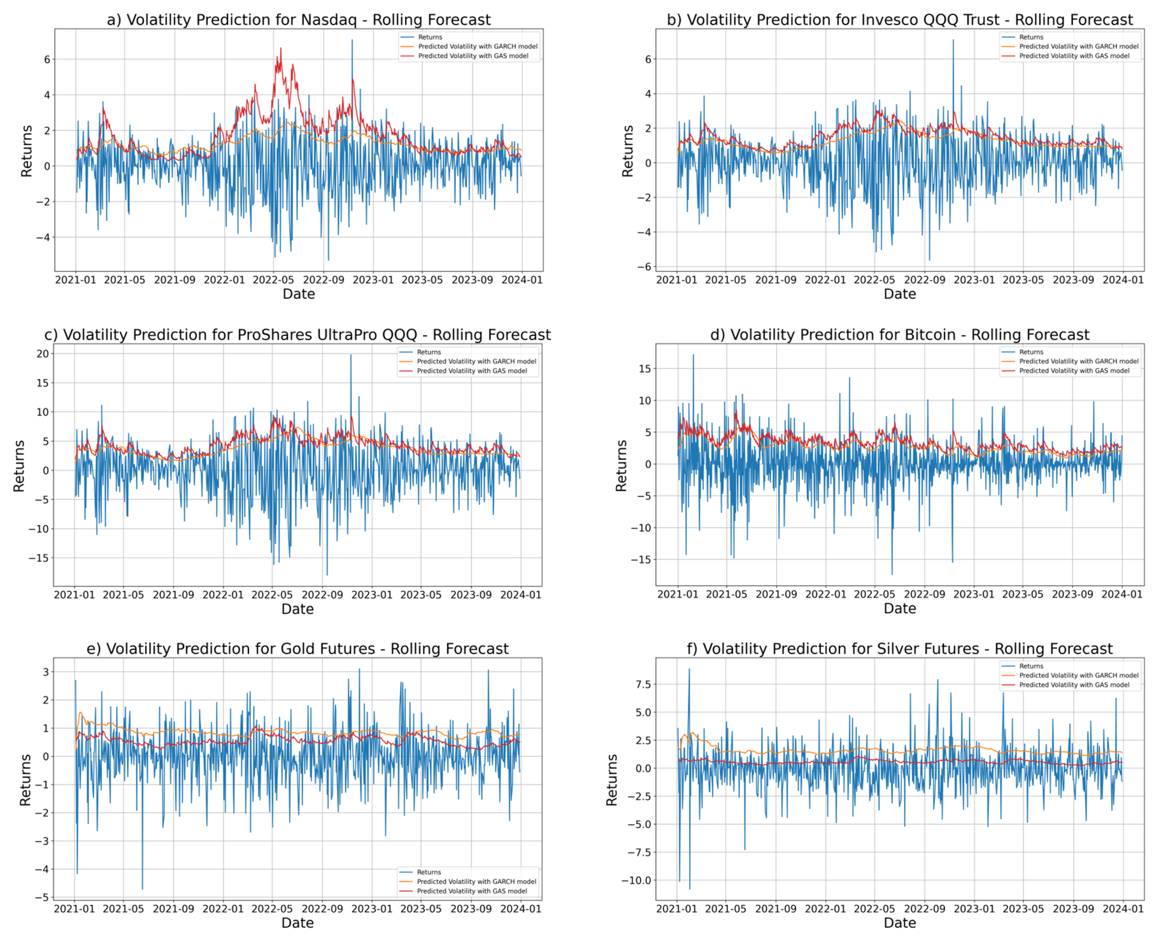
3.1. Volatility Analysis

The volatility forecasting model was implemented using the Student’s t distribution through the UniGASSpec function from the “GAS” package in RStudio, specifying a GAS(1,1) structure. Parameter estimation and forecasting were carried out using the UniGASRoll function, fitting the model to the returns of the selected financial indices. A rolling window approach was also employed to continuously update the model with the most recent data a critical feature in highly dynamic financial markets, where volatility patterns can shift abruptly [30].
Table 2 presents the time horizon used for both model calibration and volatility prediction.
Figure 5 presents the daily evolution of volatility from 1 January 2021 to 1 January 2024, showing how it adjusts to sudden and temporary changes in returns, which can translate into fluctuations in closing prices.
Validation tests were conducted to assess the model’s ability to capture the dynamics of volatility. For this purpose, the residuals were analyzed to verify that they met the properties of independence and lack of autocorrelation. Appendix A presents the autocorrelation (ACF) and partial autocorrelation (PACF) functions of both the residuals and their squared values. These plots demonstrate that the model adequately captures the temporal dependence structure and the variability of the returns.
In addition, two complementary statistical tests were applied to support these findings:
  • Ljung–Box test, used to detect the presence of autocorrelation in the residuals and to evaluate whether the model correctly captures the time structure of the series.
  • ARCH-LM test, applied to the squared residuals to identify potential ARCH effects, i.e., the presence of conditional heteroskedasticity not explained by the model.
The results of these tests are presented in Table 3.
The null hypothesis ( H 0 ) states that there is no significant autocorrelation up to the specified lag order. p-values greater than 0.05 indicate that H 0 cannot be rejected, suggesting the absence of autocorrelation in both the residuals and their variance. This implies that there is no evidence of remaining ARCH-type conditional heteroskedasticity. These results, summarized in Table 1, support the adequacy of the GAS model in capturing the temporal dynamics and volatility of the analyzed financial return series.

3.2. Results with a 3-Day Sliding Window

As presented in Table 4, with a 3-day moving window, the GAS-ATT-LSTM model demonstrated superior predictive performance across several financial assets. For Nasdaq, Bitcoin, and SILVER, the unidirectional GAS-ATT-LSTM consistently achieved the lowest error values across all evaluation metrics, confirming the effectiveness of combining the GAS framework with an attention mechanism to enhance sequential forecasting. In the cases of QQQ and TQQQ, the Bidirectional GAS-ATT-LSTM variant outperformed other configurations, highlighting the benefit of bidirectional temporal encoding when modeling highly volatile instruments. For GOLD, the Bidirectional LSTM produced the best results, suggesting that in certain market contexts, simpler recurrent architectures may offer sufficient predictive capacity. Overall, these results support the adaptability and robustness of the GAS-ATT-LSTM architecture across diverse asset classes.

3.3. Results with a 5-Day Sliding Window

By extending the moving window to 5 days, as shown in Table 5, the Bidirectional LSTM achieved the lowest errors for both Nasdaq and Bitcoin, suggesting that the base architecture is sufficient for short-term forecasting in these cases. For QQQ and GOLD, the Bidirectional GAS-LSTM yielded the best MAE, while the Bidirectional GAS-ATT-LSTM performed better in RMSE and MAPE for GOLD, indicating a trade-off between average accuracy and error dispersion. The TQQQ results favored the Bidirectional GAS-ATT-LSTM, highlighting the benefit of combining GAS and attention mechanisms for complex, leveraged instruments. Similarly, the GAS-ATT-LSTM outperformed all other models for SILVER, showing the value of attention in modeling fine-grained temporal dynamics. These findings suggest that optimal model complexity depends on asset characteristics and forecasting horizon.

3.4. Results with a 7-Day Sliding Window

With a 7-day moving window, the results presented in Table 6 reflect that the GAS-ATT-LSTM model achieved the lowest errors for Nasdaq and GOLD, confirming the benefit of attention-enhanced architectures in both volatile and stable assets. For QQQ, SILVER, and Bitcoin, the Bidirectional GAS-ATT-LSTM performed best, highlighting the advantage of combining bidirectional encoding with attention to capture complex temporal patterns. In contrast, the GAS-LSTM model outperformed all others for TQQQ, suggesting that the GAS component alone is highly effective for forecasting leveraged instruments. Overall, these results indicate that the optimal model configuration varies by asset and that hybrid approaches offer significant advantages when aligned with asset-specific dynamics.

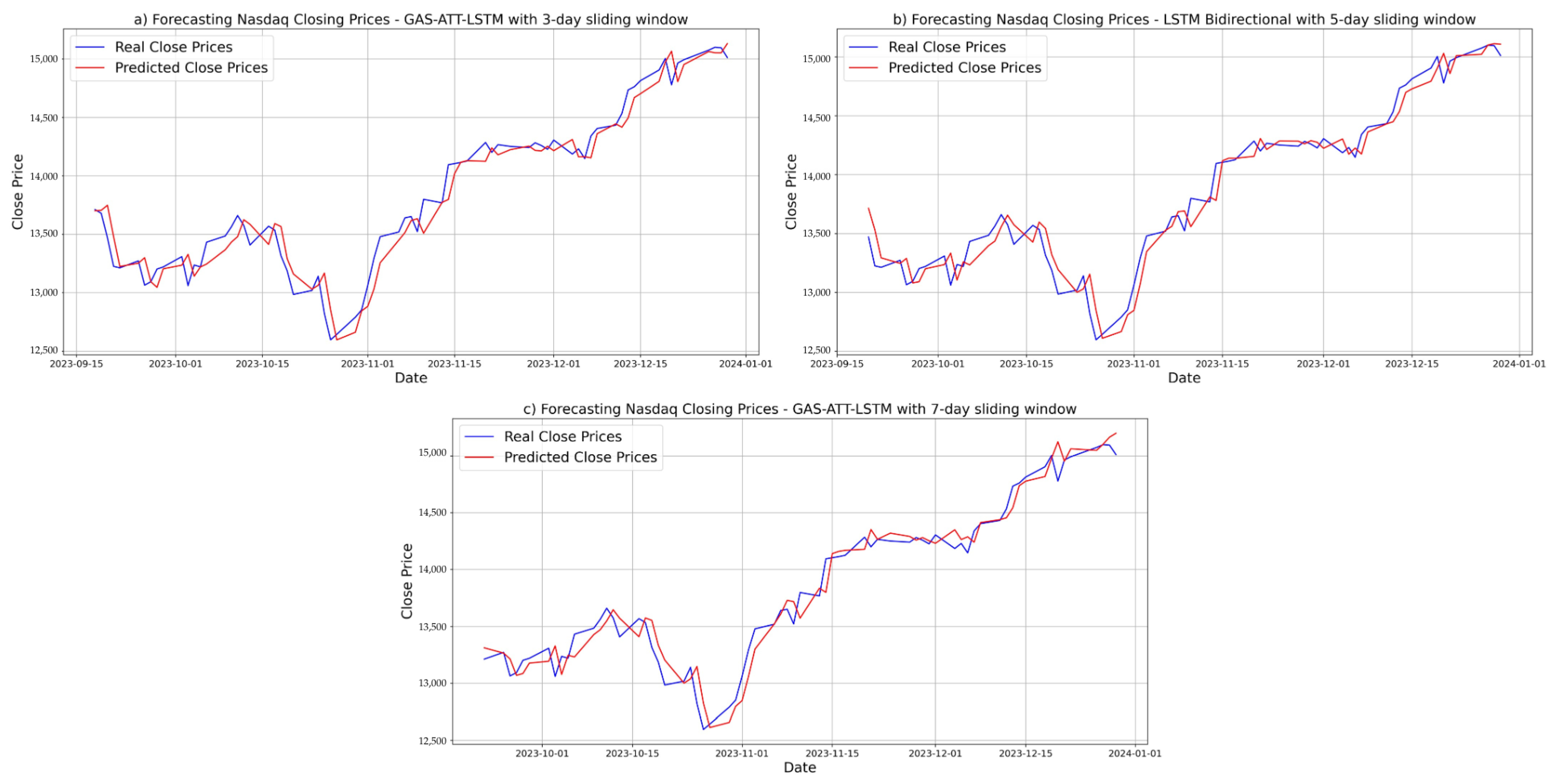
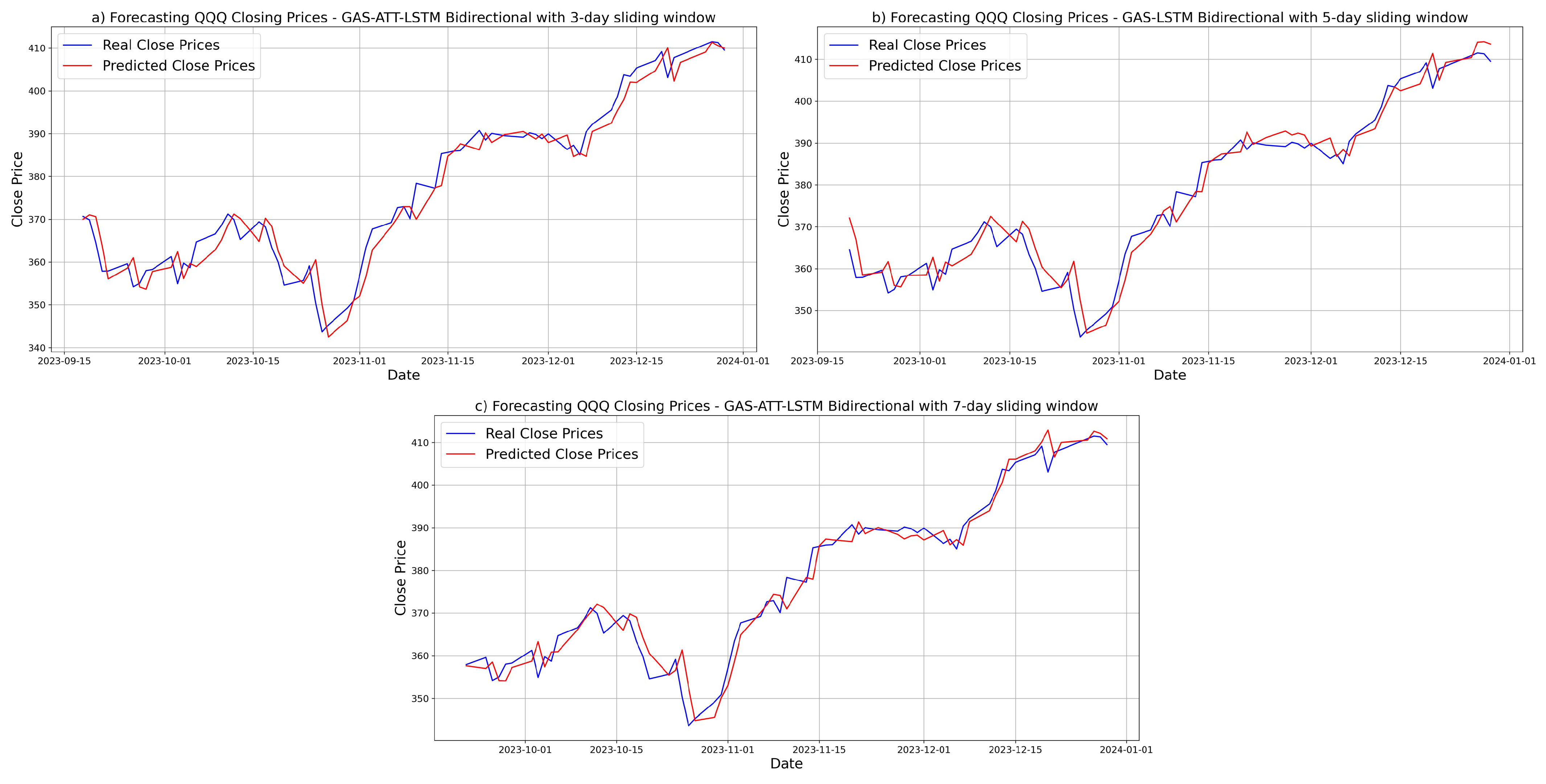
3.5. Forecasting Results and Visual Analysis

Figure 6, Figure 7, Figure 8, Figure 9, Figure 10 and Figure 11 present the forecasting results for the six financial assets. For each asset, three plots are shown, corresponding to the best-performing model under the 3-, 5-, and 7-day sliding windows. Each figure compares actual and predicted closing prices, providing a visual assessment of forecasting accuracy across different time horizons.
Appendix B presents the learning curves for the models applied to the Nasdaq series as a representative example. The curves correspond to the best-performing models under the 3, 5, and 7-day sliding windows. All models showed a consistent training behavior, with MAE and MSE decreasing rapidly during early epochs and stabilizing thereafter, indicating proper convergence without overfitting. Given the similarity in learning dynamics across assets and configurations, only the Nasdaq results are shown to avoid redundancy.

3.5.1. Prediction Results for Nasdaq

Figure 6 shows that, across all three configurations, the selected models effectively capture both the overall trend and short-term fluctuations in the Nasdaq time series. Although no systematic improvement is observed as the window size increases, the 7-day configuration yields the lowest overall prediction errors, as previously reported. These results visually confirm the capability of the GAS-ATT-LSTM model to represent the temporal dynamics of financial assets.

3.5.2. Prediction Results for QQQ

Figure 7 shows that the GAS-ATT-LSTM Bidirectional model achieved the best performance in the 3 and 7-day configurations, recording the lowest errors across all metrics. This highlights the effectiveness of combining attention mechanisms with bidirectional recurrence for stock price forecasting. Although the GAS-LSTM without attention performed competitively in the 5-day setup, the inclusion of attention clearly improved accuracy, particularly in capturing short-term variations in the QQQ series.

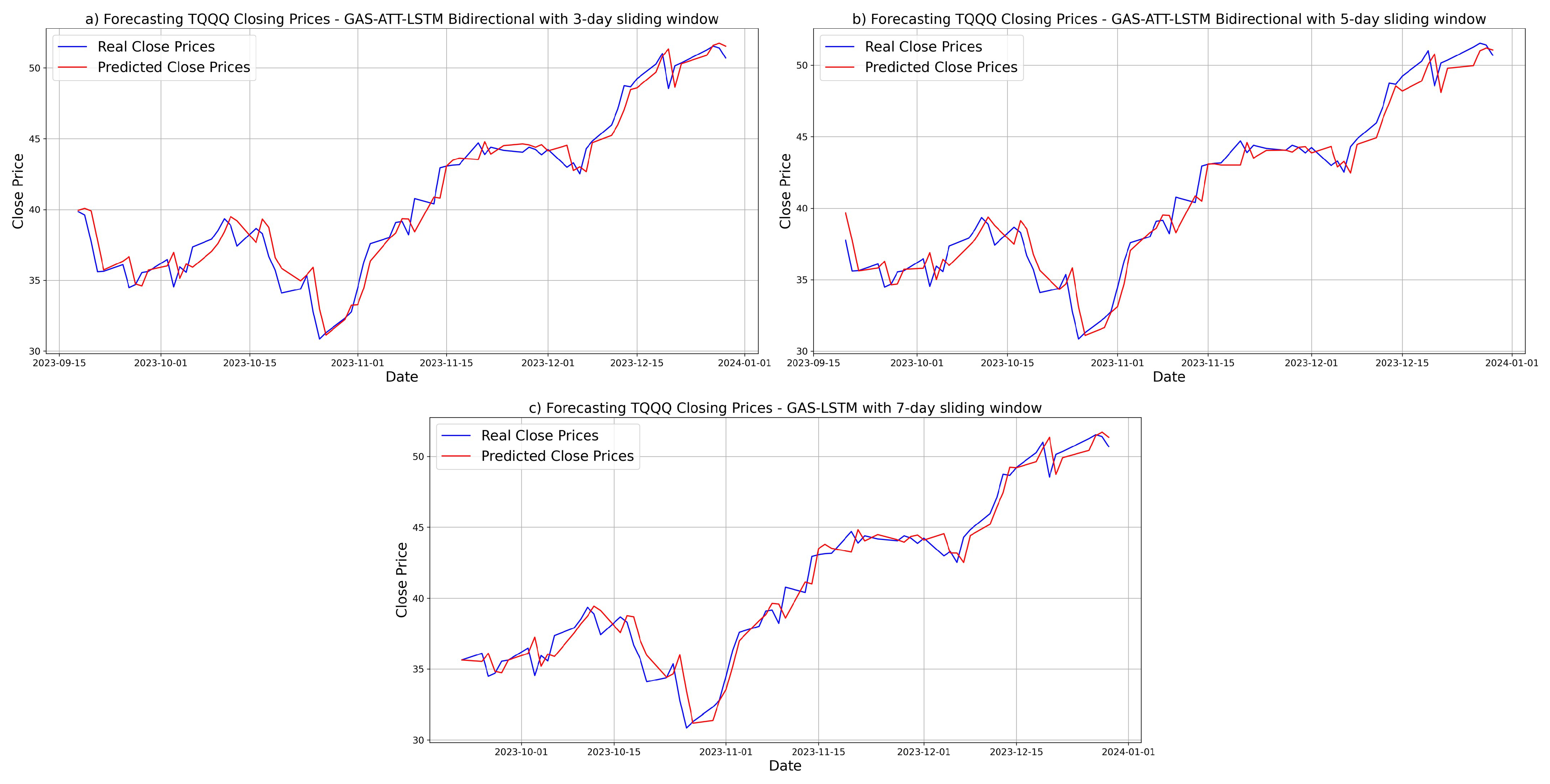
3.5.3. Prediction Results for TQQQ

Figure 8 shows that the GAS-ATT-LSTM Bidirectional model achieved the lowest errors for the 3 and 5-day windows, highlighting its effectiveness in short-term forecasting of highly volatile, leveraged assets like TQQQ. However, for the 7-day window, the simpler GAS-LSTM model without attention or bidirectionality performed best, suggesting that greater architectural complexity does not necessarily improve accuracy over longer input horizons. These results indicate that the optimal model configuration depends on both the time window and the asset’s volatility characteristics.

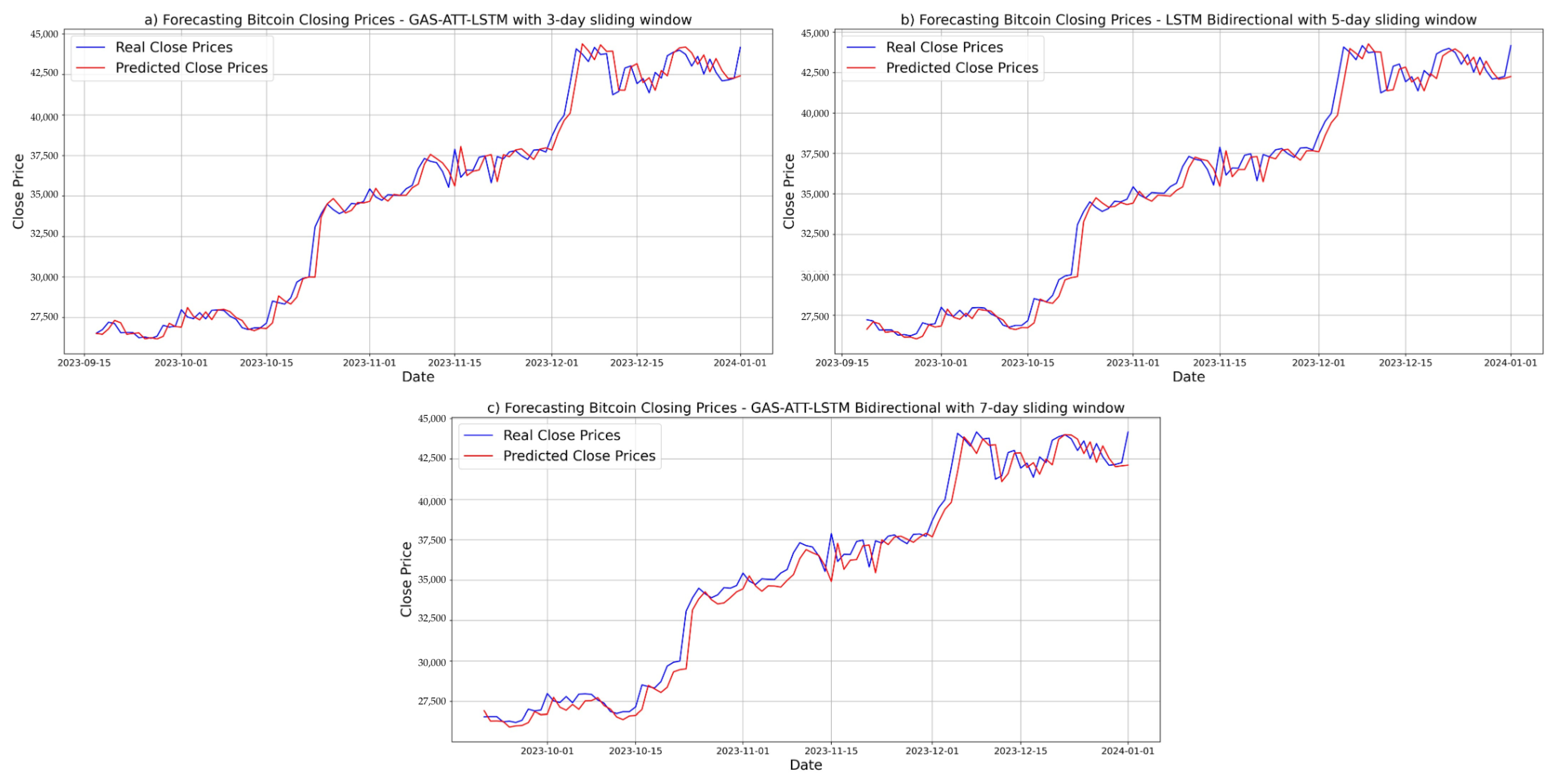
3.5.4. Prediction Results for Bitcoin

Figure 9 shows that the GAS-ATT-LSTM model achieved its highest accuracy with a 3-day window, proving especially effective for highly volatile series like Bitcoin. For the 5-day window, the bidirectional LSTM outperformed hybrid models, suggesting that simpler architectures may be more robust at intermediate horizons. With 7 days, the bidirectional GAS-ATT-LSTM yielded the lowest errors, though with a slight drop in accuracy. These results highlight the importance of aligning model architecture with the forecast horizon.

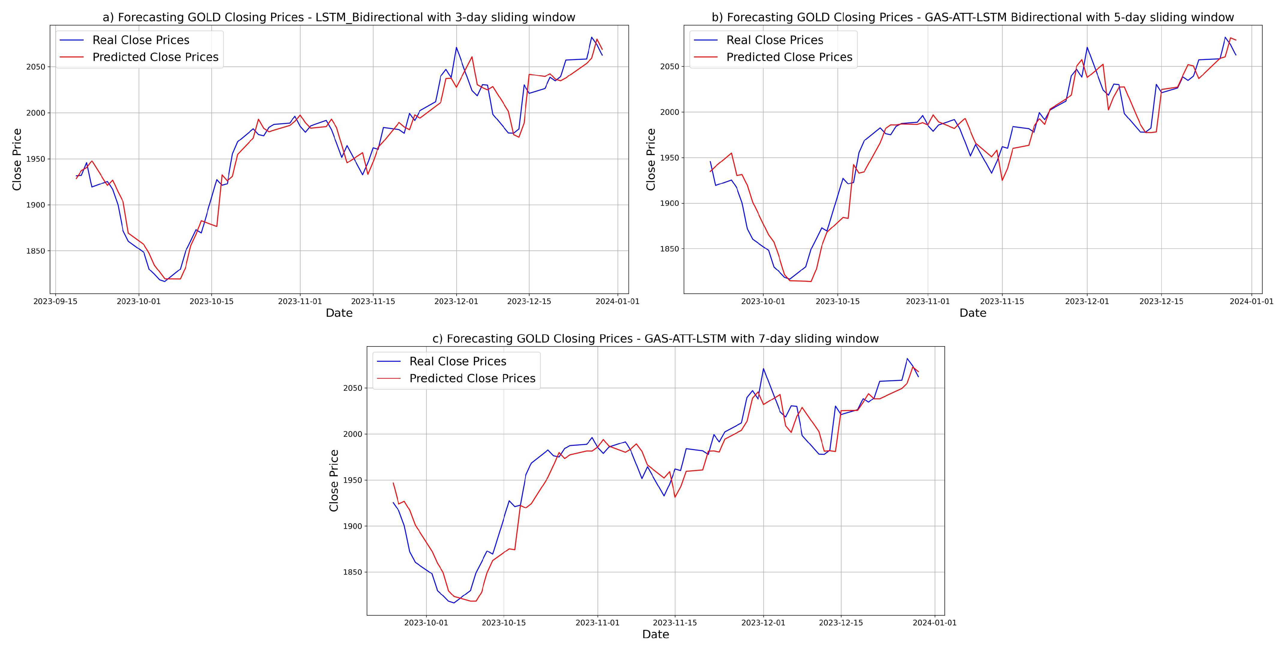
3.5.5. Prediction Results for GOLD

Figure 10 shows that with a 3-day window, the bidirectional LSTM achieved the highest accuracy, suggesting that for stable assets like GOLD, simpler models may suffice. For 5 days, the bidirectional GAS-ATT-LSTM performed best, while for 7 days, its unidirectional variant led. Although differences are minor, hybrid models remain competitive, but their advantage is less pronounced in low-volatility series.

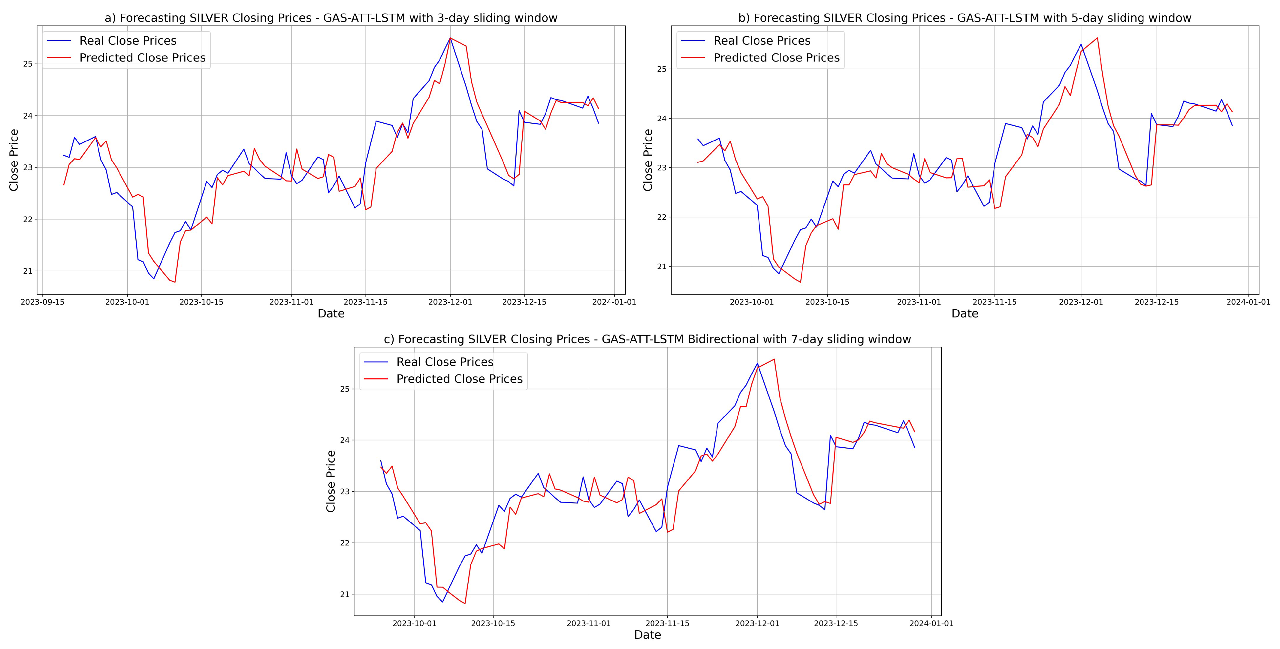
3.5.6. Prediction Results for SILVER

Figure 11 shows that the GAS-ATT-LSTM model achieved the best performance with 3-day and 5-day windows, confirming the effectiveness of the attention mechanism in modeling SILVER prices. For the 7-day window, its bidirectional variant recorded the lowest errors, suggesting that a longer historical context and richer temporal encoding can enhance accuracy. Overall, the results demonstrate that hybrid attention-based models are effective even for relatively stable assets.

3.6. Discussions

The results of this study underscore the effectiveness of hybrid architectures that combine traditional time series models with deep learning components for forecasting the daily closing prices of financial assets. The use of 3-, 5-, and 7-day sliding windows played a decisive role in predictive accuracy, with performance varying significantly across different assets.
These findings are partially consistent with the study by [3], which evaluated the performance of GARCH-ATT-LSTM structures and other variants (LSTM, LSTM-GARCH, and ATT-LSTM) for price prediction. Although their architectures are similar to those used in this work, their approach relies on a GARCH model for volatility estimation, whereas our proposal incorporates a GAS model. Moreover, Ref. [3] concluded that hybrid models performed better with 3-day and 5-day windows when forecasting the closing prices of gold futures, the Dow Jones Industrial Average, and Apple stock. In contrast, our results show that for gold futures, the Bidirectional GAS-ATT-LSTM (5-day window) and the unidirectional GAS-ATT-LSTM (7-day window) outperformed the Bidirectional GARCH-LSTM, suggesting a stronger ability of the GAS-based approach to capture market dynamics over longer forecasting horizons.
Similarly, the findings of [20] demonstrate that combining parametric models such as GARCH with deep neural networks can significantly enhance Bitcoin price forecasting. In line with this, our results show that the GAS-ATT-LSTM and its bidirectional variant, using 3-day and 7-day windows, respectively, outperformed the Bidirectional GARCH-LSTM, further validating the effectiveness of integrating GAS with attention mechanisms in highly volatile markets.
In contrast to [27], which reported that the ATT-LSTM model outperformed LSTM in predicting the Nasdaq index, our experiments reveal that the GAS-ATT-LSTM surpassed the Bidirectional LSTM for Nasdaq forecasts using both 3-day and 5-day windows. This supports the hypothesis that incorporating the GAS model alongside attention mechanisms can significantly improve predictive accuracy in financial time series, particularly under conditions of high volatility and structural complexity.
Overall, this study corroborates the conclusions drawn in [21,22], demonstrating that the integration of conventional econometric techniques with advanced machine learning frameworks can produce more accurate and effective results for identifying complex patterns in financial time series data.

4. Conclusions

This study evaluated the use of hybrid models for forecasting the daily closing prices of financial assets, with a particular focus on the GAS-ATT-LSTM architecture as the core proposal. Empirical results confirm that this architecture, especially in its bidirectional variant, delivers strong and adaptable predictive performance across a wide range of financial instruments and forecasting horizons. While simpler models, such as Bidirectional LSTM or GAS-LSTM, performed well in specific contexts (e.g., Nasdaq or TQQQ under certain window configurations), the integration of GAS dynamics with attention mechanisms consistently enhances accuracy in more complex scenarios, particularly for highly volatile assets such as QQQ, TQQQ, and SILVER. These findings also highlight the robustness of the GAS-ATT-LSTM architecture, which effectively adapts to varying market conditions and forecasting intervals, outperforming benchmark models in most scenarios and confirming its suitability for modeling diverse asset dynamics.
The limitations of this study include the manual selection of time periods, sliding windows, and hyperparameters, which may influence predictive performance. No automated optimization techniques were employed. Future work could incorporate methods such as grid search or Bayesian optimization, as well as the inclusion of exogenous variables, to enhance model accuracy and robustness.
In conclusion, this work establishes a solid foundation for future research on hybrid models applied to financial forecasting. Combining LSTM neural networks with advanced statistical models like GAS, together with an attention mechanism, shows strong potential to significantly improve financial price forecasting accuracy and strengthen methods for modeling non-stationary time series. As an extension of the present study, it is suggested to explore alternative hybrid architectures, such as GRU models, modified variants of LSTM or Transformer models integrated with the GAS framework, to assess potential improvements in predictive performance. Furthermore, incorporating exogenous macroeconomic variables (e.g., interest rates, inflation, and country risk) could enhance accuracy by capturing external drivers of volatility. Applying the model to other asset classes, such as commodities or bonds, would enable validation of its robustness across diverse financial environments. It is also recommended to evaluate its performance under extreme conditions or during periods of financial turmoil, such as the COVID-19 pandemic or recent geopolitical conflicts, to analyze its resilience in highly uncertain scenarios. Finally, the integration of intraday data (e.g., hourly prices) or the execution of a sensitivity analysis on the input window size and forecasting horizon would help tailor the model to various predictive objectives and practical applications.

Author Contributions

Conceptualization, K.A. and M.F.; methodology, K.A., M.F. and M.S.; software, K.A. and M.S.; validation, M.F., G.F. and J.V.-A.; investigation, K.A., M.F., M.S. and G.F.; resources, M.F.; data curation, K.A.; writing—original draft preparation, K.A. and M.S.; writing—review and editing, K.A., M.F., G.F. and J.V.-A.; visualization, K.A. and M.S.; supervision, M.F., G.F. and J.V.-A.; project administration, M.F.; funding acquisition, J.V.-A. All authors have read and agreed to the published version of the manuscript.

Funding

This research received no external funding.

Data Availability Statement

The data used in this article are publicly available.

Acknowledgments

The authors would like to express their gratitude to Universidad Indoamérica for its support of this research through the “Tecnologías de la Industria 4.0 en Educación, Salud, Empresa e Industria” project and to the Department of Mathematics at the Escuela Politécnica Nacional of Ecuador.

Conflicts of Interest

The authors declare no conflicts of interest.

Abbreviations

The following abbreviations are used in this manuscript:
GASGeneralized Autoregressive Score
LSTMLong Short-Term Memory
ATTAttention Mechanism
GARCHGeneralized Autoregressive Conditional Heteroscedasticity
QQQInvesco QQQ Trust
TQQQProShares UltraPro QQQ
GOLDGold futures prices
SILVERSilver futures prices
ACFAutocorrelation Function
PACFPartial Autocorrelation Function
MAEMean Absolute Error
RMSERoot Mean Squared Error
MAPEMean Absolute Percentage Error
MSEMean Squared Error

Appendix A. ACF and PACF of Residuals and Squared Residuals for the Six Financial Assets

Figure A1. ACF/PACF of Nasdaq Residuals.
Mathematics 13 02300 g0a1
Figure A2. ACF/PACF of QQQ Residuals.
Mathematics 13 02300 g0a2
Figure A3. ACF/PACF of TQQQ Residuals.
Mathematics 13 02300 g0a3
Figure A4. ACF/PACF of Bitcoin Residuals.
Mathematics 13 02300 g0a4
Figure A5. ACF/PACF of GOLD Residuals.
Mathematics 13 02300 g0a5
Figure A6. ACF/PACF of SILVER Residuals.
Mathematics 13 02300 g0a6

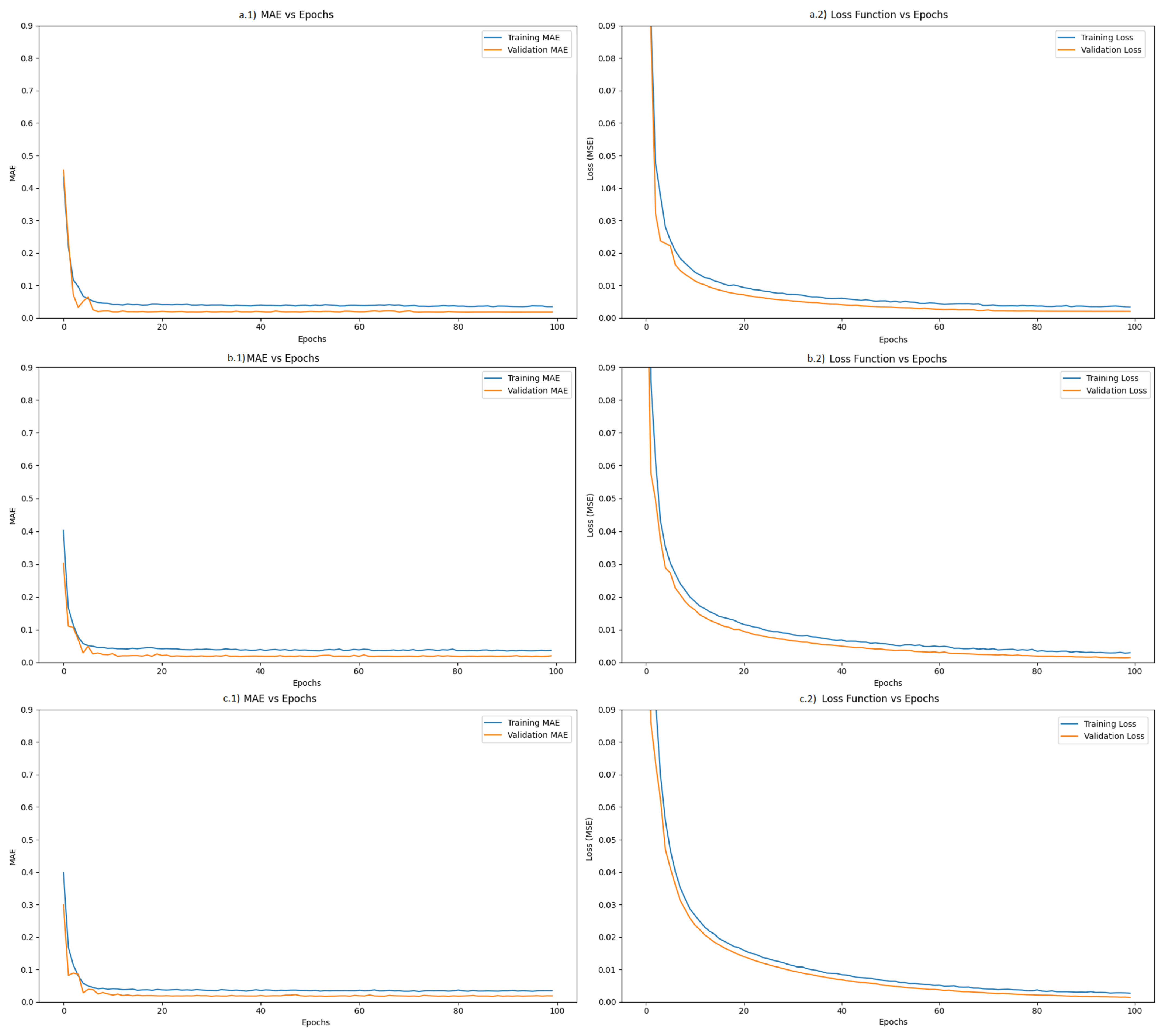
Appendix B. Learning Curves

Figure A7. MAE and loss curves for Nasdaq across models and sliding windows: (a.1,a.2) GAS-ATT-LSTM with 3-day window; (b.1,b.2) Bidirectional LSTM with 5-day window; (c.1,c.2) GAS-ATT-LSTM with 7-day window.
Mathematics 13 02300 g0a7

References

  1. Zhang, G.P.; Qi, M. Neural network forecasting for seasonal and trend time series. Eur. J. Oper. Res. 2005, 160, 501–514. [Google Scholar] [CrossRef]
  2. Cheng, C.; Sa-Ngasoongsong, A.; Beyca, O.; Le, T.; Yang, H.; Kong, Z.; Bukkapatnam, S.T.S. Time series forecasting for nonlinear and non-stationary processes: A review and comparative study. IIE Trans. 2015, 47, 1053–1071. [Google Scholar] [CrossRef]
  3. Gao, Z.; Kuruoğlu, E.E. Attention based hybrid parametric and neural network models for non-stationary time series prediction. Expert Syst. 2024, 41, e13419. [Google Scholar] [CrossRef]
  4. Di-Giorgi, G.; Salas, R.; Avaria, R.; Ubal, C.; Rosas, H.; Torres, R. Volatility forecasting using deep recurrent neural networks as GARCH models. Comput Stat. 2025, 40, 3229–3255. [Google Scholar] [CrossRef]
  5. Zhao, P.; Zhu, H.; Ng, W.S.H.; Lee, D.L. From GARCH to Neural Network for Volatility Forecast. arXiv 2024, arXiv:2402.06642. [Google Scholar] [CrossRef]
  6. Bollerslev, T. Generalized autoregressive conditional heteroskedasticity. J. Econom. 1986, 31, 307–327. [Google Scholar] [CrossRef]
  7. Engle, R.F. Autoregressive Conditional Heteroscedasticity with Estimates of the Variance of United Kingdom Inflation. Econometrica 1982, 50, 987–1007. [Google Scholar] [CrossRef]
  8. Hsieh, D.A. Nonlinear Dynamics in Financial Markets: Evidence and Implications. Financ. Anal. J. 1995, 51, 55–62. [Google Scholar] [CrossRef]
  9. Makatjane, K.D.; Xaba, D.L.; Moroke, N.D. Application of Generalized Autoregressive Score Model to Stock Returns. Int. J. Econ. Manag. Eng. 2017, 11. [Google Scholar]
  10. Creal, D.; Koopman, S.J.; Lucas, A. Generalized autoregressive score models with applications. J. Appl. Econ. 2013, 28, 777–795. [Google Scholar] [CrossRef]
  11. Harvey, A.C. Dynamic Models for Volatility and Heavy Tails: With Applications to Financial and Economic Time Series; Cambridge University Press: Cambridge, UK, 2013; pp. 8–16. [Google Scholar] [CrossRef]
  12. Cox, D.R. Statistical analysis of time-series: Some recent developments. Scand. J. Stat. 1981, 8, 110–111. [Google Scholar]
  13. Benjamin, M.A.; Rigby, R.A.; Stasinopoulos, D.M. Generalized autoregressive moving average models. J. Am. Stat. Assoc. 2003, 98, 214–223. [Google Scholar] [CrossRef]
  14. Shephard, N. Generalized Linear Autoregressions; Economics Papers; Economics Group, Nuffield College, University of Oxford: Oxford, UK, 1995. [Google Scholar]
  15. Cipollini, F.; Engle, R.; Gallo, G. Vector Multiplicative Error Models: Representation and Inference. In Econometrics Working Papers Archive; Università degli Studi di Firenze, Dipartimento di Statistica, Informatica, Applicazioni “G. Parenti”: Firenze, Italy, 2006; p. 55. [Google Scholar]
  16. Deshpande, V. Implementation of Long Short-Term Memory (LSTM) Networks for Stock Price Prediction. RJCSE 2023, 4, 60–72. [Google Scholar] [CrossRef]
  17. Gupta, P.; Malik, S.; Apoorb, K.; Sameer, S.; Vardhan, V.; Ragam, P. Stock Market Analysis Using Long Short-Term Model. EAI Endorsed Trans. Scalable Inf. Syst. 2023, 11. [Google Scholar] [CrossRef]
  18. Maknickienė, N.; Maknickas, A. Application of Neural Network for Forecasting of Exchange Rates and Forex Trading. In Proceedings of the 7th International Scientific Conference “Business and Management 2012, Vilnius, Lithuania, 10–11 May 2012. [Google Scholar] [CrossRef]
  19. Kim, H.Y.; Won, C.H. Forecasting the volatility of stock price index: A hybrid model integrating LSTM with multiple GARCH-type models. Expert Syst. Appl. 2018, 103, 25–37. [Google Scholar] [CrossRef]
  20. Gao, Z.; He, Y.; Kuruoglu, E.E. A Hybrid Model Integrating LSTM and Garch for Bitcoin Price Prediction. In Proceedings of the IEEE 31st International Workshop on Machine Learning for Signal Processing (MLSP), Gold Coast, Australia, 25–28 October 2021; pp. 1–6. [Google Scholar] [CrossRef]
  21. Kakade, K.A.; Mishra, A.K.; Ghate, K.; Gupta, S. Forecasting Commodity Market Returns Volatility: A Hybrid Ensemble Learning GARCH-LSTM Based Approach. SSRN Electron. J. 2022, 29, 103–117. [Google Scholar] [CrossRef]
  22. Verma, S. Forecasting volatility of crude oil futures using a GARCH–RNN hybrid approach. Intell. Sys. Acc. Fin. Mgmt. 2021, 28, 130–142. [Google Scholar] [CrossRef]
  23. Lipton, Z.C.; Kale, D.C.; Elkan, C.; Wetzel, R. Learning to Diagnose with LSTM Recurrent Neural Networks. arXiv 2015, arXiv:1511.03677. [Google Scholar]
  24. Bahdanau, D.; Cho, K.; Bengio, Y. Neural Machine Translation by Jointly Learning to Align and Translate. arXiv 2015, arXiv:1409.0473. [Google Scholar]
  25. Itti, L.; Koch, C. Computational modelling of visual attention. Nat. Rev. Neurosci. 2001, 2, 194–203. [Google Scholar] [CrossRef] [PubMed]
  26. Chen, Y.; Lin, W.; Wang, J.Z. A Dual-Attention-Based Stock Price Trend Prediction Model with Dual Features. IEEE Access 2019, 7, 148047–148058. [Google Scholar] [CrossRef]
  27. Zhang, X.; Liang, X.; Zhiyuli, A.; Zhang, S.; Xu, R.; Wu, B. AT-LSTM: An Attention-Based LSTM Model for Financial Time Series Prediction. IOP Conf. Ser. Mater. Sci. Eng. 2019, 569, 052037. [Google Scholar] [CrossRef]
  28. Dai, Z.; Li, J.; Cao, Y.; Zhang, Y. SALSTM: Segmented Self-Attention LSTM for Long-Term Forecasting. Res. Sq. 2024. [Google Scholar] [CrossRef]
  29. Zhang, L. LSTMGA-QPSBG: An LSTM and Greedy Algorithm-Based Quantitative Portfolio Strategy for Bitcoin and Gold. In Proceedings of the 2nd International Conference Bigdata Blockchain and Economy Management (ICBBEM) 2023, EAI, Hangzhou, China, 19–21 May 2023. [Google Scholar] [CrossRef]
  30. Ardia, D.; Boudt, K.; Catania, L. Generalized autoregressive score models in R: The GAS package. J. Stat. Softw. 2019, 88, 1–28. [Google Scholar] [CrossRef]
  31. Ahmed, M.T.; Naher, N. Modelling & Forecasting Volatility of Daily Stock Returns Using GARCH Models: Evidence from Dhaka Stock Exchange. J. Econ. Bus. 2021, 4, 74–89. [Google Scholar] [CrossRef]
  32. Ogunniran, M.O.; Tijani, K.R.; Benson, R.I.; Kareem, K.O.; Moshood, L.O.; Olayiwola, M.O. Methodological insights regarding the impact of COVID-19 dataset on stock market performance in African countries: A computational analysis. J. Amasya Univ. Inst. Sci. Technol. 2024, 5, 1–16. [Google Scholar] [CrossRef]
  33. Samuel, R.T.A.; Chimedza, C.; Sigauke, C. Framework for Simulation Study Involving Volatility Estimation: The GAS Approach. Preprints 2023, 2023061735. [Google Scholar] [CrossRef]
  34. Hochreiter, S.; Schmidhuber, J. Long Short-Term Memory. Neural Comput. 1997, 9, 1735–1780. [Google Scholar] [CrossRef] [PubMed]
  35. Ubal, C.; Di-Giorgi, G.; Contreras-Reyes, J.E.; Salas, R. Predicting the Long-Term Dependencies in Time Series Using Recurrent Artificial Neural Networks. Mach. Learn. Knowl. Extr. 2023, 5, 1340–1358. [Google Scholar] [CrossRef]
  36. Sutskever, I.; Vinyals, O.; Le, Q.V. Sequence to Sequence Learning with Neural Networks. arXiv 2014, arXiv:1409.3215. [Google Scholar] [CrossRef]
Figure 1. Historical closing prices of financial assets.
Mathematics 13 02300 g001
Figure 2. LSTM cell structure.
Mathematics 13 02300 g002
Figure 3. Structure of the GAS-ATT-LSTM model.
Mathematics 13 02300 g003
Figure 4. Temporal segmentation of data sets by financial asset.
Mathematics 13 02300 g004
Figure 5. Volatility forecasts of financial assets using the GAS model vs. the GARCH model.
Mathematics 13 02300 g005
Figure 6. Predicted Nasdaq closing prices: (a) GAS-ATT-LSTM with 3-day window, (b) LSTM Bidirectional with 5-day window, and (c) GAS-ATT-LSTM with 7-day window.
Mathematics 13 02300 g006
Figure 7. Predicted QQQ closing prices: (a) GAS-ATT-LSTM Bidirectional with 3-day window, (b) GAS-LSTM Bidirectional with 5-day window, and (c) GAS-ATT-LSTM Bidirectional with 7-day window.
Mathematics 13 02300 g007
Figure 8. Predicted TQQQ closing prices: (a) GAS-ATT-LSTM Bidirectional with 3-day window, (b) GAS-ATT-LSTM Bidirectional with 5-day window, and (c) GAS-LSTM with 7-day window.
Mathematics 13 02300 g008
Figure 9. Predicted Bitcoin closing prices: (a) GAS-ATT-LSTM with 3-day window, (b) LSTM Bidirectional with 5-day window, and (c) GAS-ATT-LSTM Bidirectional with 7-day window.
Mathematics 13 02300 g009
Figure 10. Predicted GOLD closing prices: (a) LSTM Bidirectional with 3-day window, (b) GAS-ATT-LSTM Bidirectional with 5-day window, and (c) GAS-ATT-LSTM with 7-day window.
Mathematics 13 02300 g010
Figure 11. Predicted SILVER closing prices: (a) GAS-ATT-LSTM with 3-day window, (b) GAS-ATT-LSTM with 5-day window, and (c) GAS-ATT-LSTM Bidirectional with 7-day window.
Mathematics 13 02300 g011
Table 1. Temporal and numerical distribution of data for each financial asset.
DatasetStart DateEnd DateTrainingValidationTest
Nasdaq4 January 202129 December 202352715076
QQQ4 January 202129 December 202352715076
TQQQ4 January 202129 December 202352715076
Bitcoin1 January 20211 January 2024767219110
GOLD4 January 202129 December 202352715076
SILVER4 January 202129 December 202352715076
Table 2. Estimation time ranges by financial asset. The prediction period for all assets spans from 1 January 2021 to 1 January 2024.
DatasetEstimation fromEstimation to
Nasdaq1 January 19711 January 2021
QQQ3 October 19991 January 2021
TQQQ2 November 20101 January 2021
Bitcoin17 September 20141 January 2021
GOLD30 August 20001 January 2021
SILVER30 August 20001 January 2021
Table 3. Results of Ljung–Box and ARCH-LM diagnostic tests on standardized residuals from GAS(1,1) models.
DatasetLjung–Box p-ValueARCH-LM p-ValueConclusion
( H 0 Not Rejected)
Nasdaq0.54170.4434
QQQ0.58270.5445
TQQQ0.56450.3887
Bitcoin0.52490.1343
GOLD0.17100.9955
SILVER0.17100.9955
Table 4. Model metrics with a 3-day sliding window.
DatasetModelMAERMSEMAPE (%)
NasdaqLSTM Bidirectional122.44149.010.89
GARCH-LSTM Bidirectional136.93163.950.99
ATT-LSTM125.77156.010.91
GAS-LSTM114.00144.220.83
GAS-LSTM Bidirectional115.47146.730.84
GAS-ATT-LSTM109.58142.820.80
GAS-ATT-LSTM Bidirectional135.45165.480.98
QQQLSTM Bidirectional3.1014.860.83
GARCH-LSTM Bidirectional3.1715.710.85
ATT-LSTM3.0015.140.81
GAS-LSTM3.1415.490.84
GAS-LSTM Bidirectional3.0115.090.81
GAS-ATT-LSTM3.0615.220.82
GAS-ATT-LSTM Bidirectional2.9814.290.80
TQQQLSTM Bidirectional0.911.172.32
GARCH-LSTM Bidirectional1.011.272.54
ATT-LSTM0.931.202.37
GAS-LSTM0.911.202.34
GAS-LSTM Bidirectional1.041.302.63
GAS-ATT-LSTM0.911.212.34
GAS-ATT-LSTM Bidirectional0.891.172.28
BitcoinLSTM Bidirectional585.83848.041.62
GARCH-LSTM Bidirectional558.30819.871.54
ATT-LSTM648.90919.121.80
GAS-LSTM618.75882.841.71
GAS-LSTM Bidirectional603.95860.501.69
GAS-ATT-LSTM545.70802.221.51
GAS-ATT-LSTM Bidirectional650.63926.861.79
GOLDLSTM Bidirectional12.7316.450.65
GARCH-LSTM Bidirectional15.3619.590.78
ATT-LSTM12.9816.680.66
GAS-LSTM12.9516.710.66
GAS-LSTM Bidirectional13.5517.530.69
GAS-ATT-LSTM13.9618.190.71
GAS-ATT-LSTM Bidirectional13.0916.960.66
SILVERLSTM Bidirectional0.3210.4141.390
GARCH-LSTM Bidirectional0.3130.4101.354
ATT-LSTM0.3160.4121.368
GAS-LSTM0.3120.4101.348
GAS-LSTM Bidirectional0.3170.4111.369
GAS-ATT-LSTM0.3100.4061.338
GAS-ATT-LSTM Bidirectional0.3130.4051.350
Table 5. Model metrics with a 5-day sliding window.
DatasetModelMAERMSEMAPE (%)
NasdaqLSTM Bidirectional108.38137.690.80
GARCH-LSTM Bidirectional163.49188.051.17
ATT-LSTM175.18197.731.26
GAS-LSTM116.21144.140.85
GAS-LSTM Bidirectional122.28149.940.89
GAS-ATT-LSTM112.27144.620.82
GAS-ATT-LSTM Bidirectional174.94199.551.25
QQQLSTM Bidirectional3.2916.680.88
GARCH-LSTM Bidirectional3.4518.120.92
ATT-LSTM3.5518.070.95
GAS-LSTM3.5117.690.94
GAS-LSTM Bidirectional3.1716.340.85
GAS-ATT-LSTM3.5318.080.94
GAS-ATT-LSTM Bidirectional3.8921.021.04
TQQQLSTM Bidirectional1.131.362.81
GARCH-LSTM Bidirectional1.141.372.83
ATT-LSTM1.051.262.60
GAS-LSTM1.051.262.63
GAS-LSTM Bidirectional0.941.222.41
GAS-ATT-LSTM1.081.312.68
GAS-ATT-LSTM Bidirectional0.931.182.34
BitcoinLSTM Bidirectional575.71841.101.59
GARCH-LSTM Bidirectional620.82873.191.73
ATT-LSTM607.26874.471.66
GAS-LSTM667.51940.061.81
GAS-LSTM Bidirectional1008.961287.322.74
GAS-ATT-LSTM653.17894.271.84
GAS-ATT-LSTM Bidirectional678.12940.551.88
GOLDLSTM Bidirectional12.6116.870.64
GARCH-LSTM Bidirectional13.2317.460.67
ATT-LSTM12.7616.930.65
GAS-LSTM13.6317.400.69
GAS-LSTM Bidirectional12.4116.550.63
GAS-ATT-LSTM12.3516.460.63
GAS-ATT-LSTM Bidirectional12.4416.450.63
SILVERLSTM Bidirectional0.3170.4231.362
GARCH-LSTM Bidirectional0.3180.4331.376
ATT-LSTM0.3060.4271.319
GAS-LSTM0.3070.4221.327
GAS-LSTM Bidirectional0.3100.4271.335
GAS-ATT-LSTM0.3050.4281.311
GAS-ATT-LSTM Bidirectional0.3160.4351.355
Table 6. Model metrics with a 7-day sliding window.
DatasetModelMAERMSEMAPE (%)
NasdaqLSTM Bidirectional108.93138.350.80
GARCH-LSTM Bidirectional125.92150.210.91
ATT-LSTM106.67135.960.78
GAS-LSTM124.48148.490.91
GAS-LSTM Bidirectional111.36137.550.81
GAS-ATT-LSTM104.10134.710.76
GAS-ATT-LSTM Bidirectional149.32171.811.08
QQQLSTM Bidirectional3.0013.920.80
GARCH-LSTM Bidirectional3.2415.420.86
ATT-LSTM2.8613.750.77
GAS-LSTM2.9614.560.79
GAS-LSTM Bidirectional3.6417.980.97
GAS-ATT-LSTM4.0521.081.08
GAS-ATT-LSTM Bidirectional2.6813.030.72
TQQQLSTM Bidirectional0.981.202.47
GARCH-LSTM Bidirectional1.021.242.57
ATT-LSTM1.021.292.55
GAS-LSTM0.841.122.15
GAS-LSTM Bidirectional0.881.152.26
GAS-ATT-LSTM1.301.493.22
GAS-ATT-LSTM Bidirectional1.051.312.60
BitcoinLSTM Bidirectional631.93885.571.72
GARCH-LSTM Bidirectional635.32882.551.79
ATT-LSTM722.13993.651.96
GAS-LSTM627.68863.261.74
GAS-LSTM Bidirectional606.07861.481.68
GAS-ATT-LSTM655.51914.131.83
GAS-ATT-LSTM Bidirectional602.90857.421.66
GOLDLSTM Bidirectional14.2418.100.72
GARCH-LSTM Bidirectional13.4717.460.68
ATT-LSTM14.0117.920.71
GAS-LSTM14.6318.970.74
GAS-LSTM Bidirectional13.3417.470.68
GAS-ATT-LSTM13.0117.180.66
GAS-ATT-LSTM Bidirectional14.3218.470.72
SILVERLSTM Bidirectional0.3120.4181.343
GARCH-LSTM Bidirectional0.3160.4191.365
ATT-LSTM0.2990.4091.291
GAS-LSTM0.3180.4221.373
GAS-LSTM Bidirectional0.3060.4151.316
GAS-ATT-LSTM0.2980.4191.281
GAS-ATT-LSTM Bidirectional0.2960.4061.273
Disclaimer/Publisher’s Note: The statements, opinions and data contained in all publications are solely those of the individual author(s) and contributor(s) and not of MDPI and/or the editor(s). MDPI and/or the editor(s) disclaim responsibility for any injury to people or property resulting from any ideas, methods, instructions or products referred to in the content.

