Credit Rating Model Based on Improved TabNet

Abstract

Under the rapid evolution of financial technology, traditional credit risk management paradigms relying on expert experience and singular algorithmic architectures have proven inadequate in addressing complex decision-making demands arising from dynamically correlated multidimensional risk factors and heterogeneous data fusion. This manuscript proposes an enhanced credit rating model based on an improved TabNet framework. First, the Kaggle “Give Me Some Credit” dataset undergoes preprocessing, including data balancing and partitioning into training, testing, and validation sets. Subsequently, the model architecture is refined through the integration of a multi-head attention mechanism to extract both global and local feature representations. Bayesian optimization is then employed to accelerate hyperparameter selection and automate a parameter search for TabNet. To further enhance classification and predictive performance, a stacked ensemble learning approach is implemented: the improved TabNet serves as the feature extractor, while XGBoost (Extreme Gradient Boosting), LightGBM (Light Gradient Boosting Machine), CatBoost (Categorical Boosting), KNN (K-Nearest Neighbors), and SVM (Support Vector Machine) are selected as base learners in the first layer, with XGBoost acting as the meta-learner in the second layer. The experimental results demonstrate that the proposed TabNet-based credit rating model outperforms benchmark models across multiple metrics, including accuracy, precision, recall, F1-score, AUC (Area Under the Curve), and KS (Kolmogorov–Smirnov statistic).

1. Introduction

With the advent of the internet era, the credit business of financial institutions has been continuously developing, bringing significant profits while also creating higher demands for the management and control of credit risk. Credit risk is a major risk that every financial institution must guard against. If not effectively managed, it can trigger a series of financial and operational risks, causing substantial losses for financial institutions. A good credit risk prediction model enables financial institutions to accurately identify potential defaulting customers, thereby mitigating risks and achieving higher profits, making it of great research significance.

Credit rating is one of the earliest financial risk management tools and one of the most successful applications of statistics and machine learning in finance [1]. Credit rating is a complete set of decision support techniques that assist lending institutions in issuing consumer credit. It improves the efficiency of information transmission, and the quantitative results can replace the highly subjective descriptive language in credit reports, enabling loan officers to more easily assess the creditworthiness of borrowers [2]. In the 1980s, logistic regression became the primary tool for credit rating [3]. With the continuous development of data mining techniques, methods such as neural networks, support vector machines, and random forests began to emerge as mainstream scoring tools [4,5,6].

Rishehchi et al. [7] incorporated users’ network attributes into the model, thereby effectively improving the accuracy of machine learning models. Caruso et al. [8] applied cluster analysis to customers’ mixed feature data, and empirical results showed that cluster analysis is an effective method for credit risk assessment. Ugo Fiore et al. [9] introduced a generative adversarial network model for handling imbalanced fraud datasets. The experimental results demonstrated that the augmented dataset outperformed the classifier trained on the original data. Zahra et al. [10] utilized random forest, CatBoost, LightGBM, and XGBoost to evaluate two feature extraction methods: Principal Component Analysis and Convolutional Autoencoders. The results indicated that the combination of Convolutional Autoencoders with random under-sampling achieved the best performance in credit rating. ZY et al. [11] propose a novel credit scoring model called the transductive semi-supervised metric network. The results indicate that the transductive semi-supervised metric network can overcome sample selection bias and more accurately classify credit applicants. Li, XT et al. [12] mainly studies the application of the radial basis function neural network model combined with the optimal segmentation algorithm in the personal loan credit rating model of banks or other financial institutions. The optimal segmentation algorithm is applied to the training of RBF neural network parameters to increase the center and width of the class.

With the continuous evolution of machine learning algorithms, researchers have gradually recognized the performance bottlenecks of single models in complex tasks, such as XGBoost, LightGBM and CatBoost. Although traditional statistical models offer certain reliability and stability, they exhibit significant limitations when handling large volumes of high-dimensional, uncertain, and nonlinear data [13]. This realization has driven significant advancements in ensemble learning theory. In the development path of Boosting techniques, a series of algorithms using decision trees as base models have achieved important breakthroughs, from the classic GBDT (Gradient Boosting Decision Tree) to subsequent improved algorithms such as XGBoost, LightGBM, and CatBoost [14,15,16,17]. Among them, XGBoost has become a milestone algorithm in this field due to its comprehensive advantages in prediction accuracy, computational efficiency, and scalability.

TabNet [18] is a deep learning model introduced by Google Cloud AI in 2021, specifically designed for tabular data. It combines the end-to-end learning capability of deep neural networks with features such as sparse feature selection and interpretability found in tree-based models. Asencios et al. [19] developed six profit scoring models capable of predicting the Internal Rate of Return of credit applications using multilayer perceptron, XGBoost, and TabNet algorithms, thereby serving as a support tool for credit analysts. Mametkulov [20] proposed a nonlinear feature representation method combining TabNet with the Hurst exponent and Lyapunov exponent for memory-related decoding. Through comparative experiments, the proposed composite model demonstrated excellent performance and interpretability. Wang et al. [21] addressed the limitations of existing photovoltaic forecasting models, which are constrained by uncertainty and intermittency. They proposed a novel hybrid deep learning model based on TabNet and linear regression, expanding the original feature space and uncovering implicit temporal relationships between features. Validation with real-world data confirmed that the proposed model achieved optimal performance. Kanász et al. [22] introduced multiple loss functions into the TabNet architecture to improve its handling of high-dimensional and heterogeneous data. These modifications enhanced the model’s sensitivity to minority classes and improved overall prediction accuracy for imbalanced datasets. McDonnell et al. [23] found that TabNet requires substantial time and effort for hyperparameter tuning. Despite these challenges, TabNet outperformed XGBoost and Logistic Regression models, providing better pricing models for interpretable models in insurance. TabNet excels at handling low-dimensional sparse tabular data. Although it offers interpretability, this characteristic somewhat limits the performance of TabNet.

Notably, existing studies often limit themselves to simple two-layer stacking of Boosting family algorithms like XGBoost and LightGBM with Logistic Regression [24]. This traditional paradigm exhibits significant limitations in feature interaction modeling and model diversity. In contrast, the Stacking ensemble method, through its unique hierarchical architecture, effectively integrates the complementary advantages of heterogeneous models, demonstrating substantial potential in enhancing classification performance [25]. Xie et al. [26] validated the feasibility of Stacking ensemble learning using XGBoost, LightGBM, CatBoost, and TabNet, achieving significant improvements in Mean Absolute Error and Mean Relative Error.

In order to overcome the technical bottlenecks of existing single-model credit risk assessment, enhance TabNet’s ability to capture features from high-dimensional, dense datasets, and further improve financial institutions’ risk identification and control capabilities during the pre-loan review phase, the present manuscript undertakes the following research.

This manuscript proposes a Stacking ensemble learning model based on an enhanced TabNet architecture, along with a Bayesian optimization-driven automated hyperparameter search method for TabNet. The improved TabNet incorporates a multi-head attention mechanism to better handle high-dimensional dense datasets. A Stacking framework is adopted, where XGBoost, LightGBM, CatBoost, KNN, and SVM are selected as base learners in the first layer. The first-layer models consist of multiple individual classifiers, while XGBoost serves as the meta-learner in the second layer. Finally, the enhanced model is evaluated on Kaggle’s “Give Me Some Credit” dataset, with performance metrics including accuracy, precision, recall, F1-score, AUC, and KS [27].

The research in this manuscript makes contributions to the existing literature in three aspects. First, to the best of our knowledge, we are the first to conduct credit scoring based on the Stacking ensemble learning of the TabNet model in the field of financial academia. Unlike most studies focusing on traditional econometric models, we innovatively introduce a non-linear machine learning model based on ensemble learning for credit scoring, filling the gap in the application of Stacking ensemble learning in the field of credit scoring. Second, our model achieves a significant performance improvement through Bayesian optimization, multi-head attention mechanism, and ensemble learning, which also validates the arguments about ensemble learning in the existing financial literature. Finally, the experimental results show that the model in this manuscript can be applied to the actual credit risk identification and control, providing a scientific decision-making basis for financial institutions to take preventive measures in advance, thereby reducing the risk of default and even the generation of non-performing loans.

Section 2 of this manuscript provides an introduction to existing credit rating models, primarily including Boosting family models such as XGBoost, LightGBM, CatBoost, the TabNet model, and Stacking ensemble learning. Section 3 presents the detailed design of the proposed improved TabNet credit rating model. Section 4 discusses the experimental design and analysis of the results. Section 5 provides the conclusion.

2. Credit Rating Model

Credit rating is one of the earliest financial risk management tools, adopted by American retailers and mail-order companies as early as the 1950s. Credit rating is a process that uses statistical models to convert relevant data into numerical measures, aimed at assessing the credit risk level of borrowers. This numerical measure is typically used to guide credit decisions, helping financial institutions more accurately evaluate the creditworthiness of borrowers, thereby reducing risk, optimizing the asset–liability structure, and improving profitability.

2.1. Boosting Models

2.1.1. XGBoost Model

XGBoost is an efficient implementation of GBDT and an ensemble learning method. Based on GBDT, the algorithm introduces L1 and L2 regularization terms and supports parallel processing, thereby improving the model’s training speed and reducing the risk of overfitting. The overall approach is to iteratively increase the number of decision trees, gradually approaching the true values.

XGBoost is an additive model that sums over $k$ base learners. The model after $t$ iterations is expressed as Equation (1).

$${\widehat{y}}_i^{(t)}={\displaystyle \sum _{k=1}^t{f}_k(x_i)={\widehat{y}}_i^{(t-1)}+f_t(x_i)}$$

(1)

XGBoost adds the loss function and the regularization term to obtain the objective function, which is expressed as Equation (2).

$$L(\Phi )={\displaystyle \sum _i^{n}l({\widehat{y}}_i,y_i)+{\displaystyle {\sum }_k^K\Omega (f_k)}}$$

(2)

In the equation, $i$ represents the $i$-th sample in the overall dataset; $n$ denotes the total number of samples used when training the $k$-th tree; $K$ represents the total number of trees trained; the loss function $L$ indicates the error between the true value and the predicted value of the $i$-th sample; ${\displaystyle {\sum }_k^K\Omega (f_k)}$ is the regularization term, which represents the complexity of the $K$ trees, with smaller values indicating stronger model generalization. By performing a second-order Taylor expansion of the loss function, Equation (3) is obtained.

$$f(x+\Delta x)\approx f(x)+f^{\prime }(x)\Delta x+{\displaystyle \frac{1}{2}}{f}^{″}(x)\Delta x^2$$

(3)

For computational convenience, define the variables $g_i$ and $h_i$ as given in Equations (4) and (5).

$$g_i={\partial }_{{\widehat{y}}_i^{(t-1)}}l(y_i,{\widehat{y}}_i^{(t-1)})$$

(4)

$$h_i={\partial }_{{\widehat{y}}_i^{(t-1)}}^{2}l(y_i,{\widehat{y}}_i^{(t-1)})$$

(5)

The objective function, after simplification, can be approximated by Equation (6).

$$Ob{j}^{(t)}\approx {\displaystyle \sum _{i=1}^n[l(y_i,{\widehat{y}}_i^{(t-1)})+g_i{f}_t(x_i)+\frac{1}{2}{h}_i{f}_t^2(x_i)]}+\Omega (f_t)+u$$

(6)

When the objective function is defined by a decision tree, XGBoost maps a single sample to the leaf node of the tree structure, which leads to Equation (7).

$$f_t(x)=w_{q(x)},w\in R^T,q:R^d\to \{1,2,\dots ,T\}$$

(7)

The regularization term in the XGBoost objective function contains a vector composed of the number of leaf nodes of the decision tree and their corresponding weights. The complexity of the decision tree is determined by the number of leaf nodes, $T$. Therefore, the expression for the tree complexity, $\Omega$, is given by Equation (8).

$$\Omega (f_t)=\gamma T+{\displaystyle \frac{1}{2}}\lambda {\displaystyle \sum _{j=1}^T{w}_j^2}$$

(8)

In the above equation, $\gamma$ and $\lambda$ are weight parameters that control the number of leaves, and $w_j$ is the value of the $j$-th leaf node. By simplifying the loss function into the form of leaf nodes, Equation (9) can be obtained.

$$\begin{array}{ll}Ob{j}^{(t)}& \simeq {\displaystyle \sum _{i=1}^n[g_i{f}_t(x_i)+\frac{1}{2}{h}_i{f}_t^2(x_i)]}+\Omega (f_t)\\ & ={\displaystyle \sum _{i=1}^n[g_i{w}_{q(x_i)}+\frac{1}{2}{h}_i{w}_{q(x_i)}^2]}+\gamma T+{\displaystyle \frac{1}{2}}\lambda {\displaystyle \sum _{j=1}^T{w}_j^2}\\ & ={\displaystyle \sum _{j=1}^T[({\displaystyle \sum _{i\in I_j}{g}_i})w_j+\frac{1}{2}({\displaystyle \sum _{i\in I_j}{h}_i}+\lambda )w_j^2]+\gamma T}\end{array}$$

(9)

The transformation can be performed using Equation (10).

$$G_j={\displaystyle \sum _{i\in I_j}{g}_i},H_j={\displaystyle \sum _{i\in I_j}{h}_i}$$

(10)

In the equation, $G_j$ represents the sum of the first-order derivatives of the samples in the $j$-th leaf node, and $H_j$ represents the sum of the second-order derivatives of the samples in the $j$-th leaf node. Therefore, the XGBoost objective function can be further simplified to Equation (11).

$$Ob{j}^{(t)}={\displaystyle \sum _{j=1}^T[G_j{w}_j+\frac{1}{2}(H_j+\lambda )w_j^2]+\gamma T}$$

(11)

Using the formula for finding the extreme values of a quadratic equation, the value of $w_j$ that minimizes the objective function is given by Equation (12).

$$w_j^{*}=-{\displaystyle \frac{G_j}{H_j+\lambda }}$$

(12)

The final loss function of the XGBoost model is given by Equation (13).

$$Obj=-{\displaystyle \frac{1}{2}}{\displaystyle \sum _{j=1}^T\frac{G_j^2}{H_j+\lambda }+\gamma }T$$

(13)

XGBoost, as a highly optimized gradient boosting framework, employs a sparsity-aware node splitting strategy and an approximate algorithm based on weighted quantile sketch, significantly improving memory efficiency and computational parallelism [28]. It performs well on both classification and regression tasks, demonstrating strong predictive capabilities across numerous datasets. However, without appropriate regularization measures, it is prone to overfitting. Moreover, as a tree-based algorithm, XGBoost cannot directly process textual data and requires text to be encoded into numerical features before training.

XGBoost uses the Scikit-learn API for parameter tuning. In this manuscript, a grid search approach was employed to identify the optimal combination of model hyperparameters. The hyperparameter distribution ranges of XGBoost are determined based on model initialization configurations and empirical values established in prior research. After parameter optimization, the final parameter settings for the model are as follows: number of subtrees, n_estimators = 200; tree depth, max_depth = 5; minimum sample weight in the child nodes, min_child_weight = 1; training set proportion, subsample = 0.8; learning rate, learning_rate = 0.06.

2.1.2. LightBGM Model

LightGBM is an efficient gradient boosting framework developed by Microsoft Corporation, specifically designed for the fast processing of large-scale datasets. This framework is based on the GBDT algorithm and has been significantly optimized to address the performance bottlenecks of traditional GBDT when handling massive amounts of data. Specifically, LightGBM introduces innovative techniques such as the histogram-based decision tree algorithm, gradient-based one-side sampling, and exclusive feature bundling, which greatly enhance model training efficiency while maintaining high predictive accuracy. Its unique feature parallelism and data parallelism strategies allow the framework to perform excellently when processing high-dimensional sparse data, making it particularly suitable for large-scale machine learning tasks. Additionally, LightGBM supports various machine learning tasks, including multi-class classification, ranking, and regression, and has gained widespread application and recognition in both industry and academia.

The histogram algorithm is a computational method that optimizes decision tree training efficiency through feature discretization. Its core principle is to divide continuous feature values into several discrete intervals and quickly determine the optimal feature split points based on bucketed statistical information. Specifically, the algorithm first performs bucketing on each continuous feature, dividing the value range into $k$ intervals. Then, it traverses all samples, counting the sum of gradients, the sum of second-order derivatives, and the number of samples within each bucket, forming global or local statistical histograms. During decision tree node splitting, the algorithm does not need to traverse all original data points but directly uses the statistical differences between adjacent buckets in the histogram, such as information gain or mean squared error, to evaluate the quality of potential split points. This mechanism significantly reduces computational overhead, compresses memory usage through bucketing, and simultaneously introduces a certain regularization effect.

The core idea of gradient-based one-side sampling is to reduce the computational cost while preserving model accuracy through a gradient-sensitive data sampling strategy. Specifically, gradient-based one-side sampling is based on the following observation: during the gradient boosting process, samples with larger absolute gradients contribute more significantly to information gain, while low-gradient samples have a smaller impact on model updates. LightGBM achieves efficient sampling through the following steps.

Gradient sorting and sampling: The absolute gradients of all samples in the current model are sorted, retaining the top $a\%$ of high-information samples with the largest absolute gradients, while randomly selecting $b\%$ of the remaining low-gradient samples.

Weight compensation: To eliminate sampling bias, the gradient values of the randomly selected low-gradient samples are weight-compensated, i.e., their gradients are multiplied by a scaling factor $(1-a)/b$ when calculating information gain, in order to maintain the unbiasedness of the statistics.

The exclusive feature bundling algorithm aims to significantly improve model training efficiency through feature dimensionality reduction. Its core principle is based on the observation that many features in real-world scenarios are mutually exclusive, and these features can be combined into a single composite feature without resulting in loss. The basic idea of the algorithm is to group features with certain correlations into exclusive feature bundles and replace the original features with these bundled feature sets. These bundles are mutually exclusive, i.e., any given sample can belong to only one bundle, thereby reducing the model’s complexity and the amount of feature computation required. The specific implementation process is as follows.

Step 1: Compute the pairwise correlations among all features and perform clustering based on feature similarity to group highly correlated features into the same package.

Step 2: For each feature package, select a representative feature, calculate the inter-feature correlation coefficients or mutual information, and determine the optimal threshold for fusing features within that package.

Step 3: Compare each feature package against the others and conduct a final selection by computing a score for each package, retaining the package with the highest score.

Step 4: Generate new features based on the selected feature packages, replacing the original features with these packages.

LightGBM exhibits significant advantages in efficiency and scalability by employing histogram-based algorithms and leaf-wise growth strategies, which substantially reduce memory consumption and computational costs while maintaining competitive accuracy. Its support for parallel computing, categorical feature handling, and gradient-based sampling further enhance performance in large-scale datasets. However, the algorithm’s potential overfitting on noisy datasets, and precision loss from feature discretization, represent notable limitations [29]. These characteristics necessitate careful regularization and parameter optimization in practical implementations.

LightGBM uses the Scikit-learn API for parameter tuning. In this manuscript, a grid search approach was employed to identify the optimal combination of model hyperparameters. The hyperparameter distribution ranges of LightBGM are determined based on model initialization configurations and empirical values established in prior research. After parameter optimization, the final parameter settings for the model are as follows: number of subtrees, n_estimators = 200; tree depth, max_depth = 8; minimum sample weight in the child nodes, min_child_weight = 8.5; number of leaves, num_leaves = 235; learning rate, learning_rate = 0.06; L1 regularization coefficient, reg_alpha = 0.5; L2 regularization coefficient, reg_lambda = 5.72.

2.1.3. CatBoost Model

CatBoost is an ensemble learning algorithm that is designed to efficiently handle categorical features and reduce the risk of overfitting. Through innovative feature encoding strategies, an ordered gradient boosting mechanism, and a symmetric tree structure design, CatBoost significantly improves model performance and training efficiency in heterogeneous data scenarios. It has now become one of the benchmark tools in high-dimensional sparse data fields such as financial risk control and recommendation systems.

CatBoost proposes an innovative categorical feature encoding framework that combines adaptive target statistics with Bayesian prior regularization to achieve automated high-precision mapping of categorical variables to numerical variables. Compared to traditional methods that rely on manual encoding, this framework constructs categorical features based on Equation (14).

$$TS(x_i^k)={\displaystyle \frac{{\displaystyle {\sum }_{j=1}^N\parallel (x_j^k=x_i^k)y_j+\alpha p}}{{\displaystyle {\sum }_{j=1}^N\parallel (x_j^k=x_i^k)+\alpha }}}$$

(14)

$\alpha$ is the smoothing coefficient, $p$ is the global target mean, and $\parallel (·)$ is the indicator function. This equation effectively alleviates the overfitting issue in low-frequency categories caused by insufficient samples in Greedy Target-based Statistics by introducing a Dirichlet prior distribution.

In the GBDT framework, the autocorrelation of training data can lead to Gradient Estimation Bias, which in turn causes the Prediction Shift problem. To obtain an unbiased gradient estimate, CatBoost trains a separate model $M_i$ for each sample $x_i$ using data that excludes the sample itself. This model is then used to estimate the gradient for the sample, and the estimated gradient is employed to train the base learner to obtain the final model. However, the implementation of this approach in the context of ranking-based boosting requires training $n$ different models, which significantly increases memory consumption and computational complexity, rendering it impractical for real-world applications. To address this, CatBoost introduces further optimizations during the tree construction phase through two boosting modes: Ordered and Plain, enhancing the efficiency of the Ordered Boosting algorithm.

CatBoost and LightGBM are both gradient boosting algorithms and offer greater flexibility compared to random forest. However, CatBoost demonstrates superior performance in handling categorical variables [30]. While both algorithms are suitable for large-scale and high-dimensional datasets, CatBoost excels in dealing with categorical features and missing values, whereas LightGBM offers advantages in terms of speed and accuracy.

CatBoost uses the Scikit-learn API for parameter tuning. In this manuscript, a grid search approach was employed to identify the optimal combination of model hyperparameters. The hyperparameter distribution ranges of CatBoost are determined based on model initialization configurations and empirical values established in prior research. After parameter optimization, the final parameter settings for the model are as follows: number of iterations, iterations = 300; tree depth, max_depth = 5; maximum size for One Hot encoding, one_hot_max_size = 1; learning rate, learning_rate = 0.04; L2 regularization coefficient, l2_leaf_reg = 3.

2.2. TabNet Model

The TabNet model, proposed by Google Cloud AI in 2021, is the first self-supervised deep learning model for tabular data. The model fully incorporates the advantages of existing tree models and DNN models, integrating the ideas of both to achieve excellent model performance and interpretability. TabNet can directly input raw tabular features without any feature preprocessing, which is not possible with tree models. Additionally, it is trained using gradient descent to achieve end-to-end learning. Therefore, this manuscript chooses to use TabNet as the initial model for training.

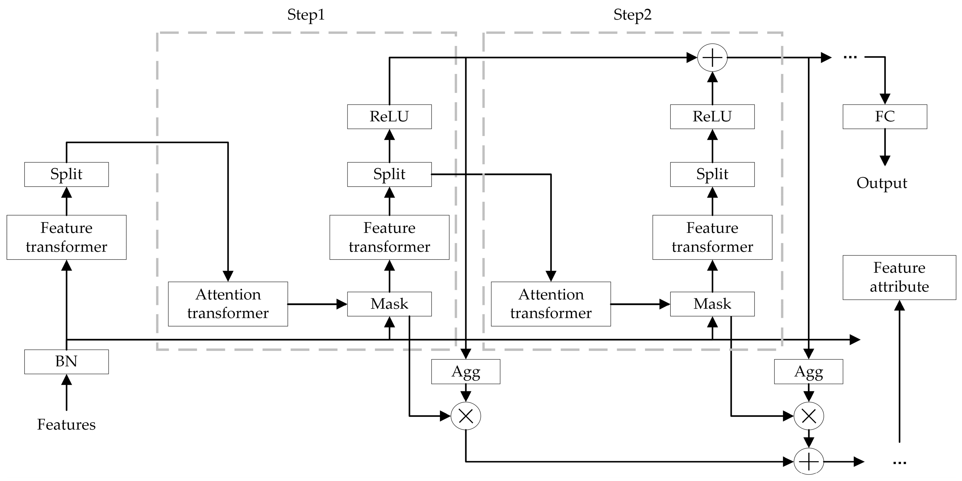
The core principle of TabNet is based on a collaborative mechanism of multi-step feature selection and information aggregation. The model generates sparse feature masks at each decision step using attention transformers, dynamically selecting important subsets of features, and encodes the selected features into higher-order representations using feature transformers. These representations are progressively merged through residual connections to form global feature interaction information. Finally, the model outputs the decision results through a Softmax function. A significant advantage of TabNet is its interpretability, as the feature selection process provides a clear weight distribution, making it easier to understand the model’s decision-making basis. Furthermore, its computational complexity is low, making it suitable for large-scale tabular data scenarios. The TabNet network structure is shown in Figure 1.

TabNet is an overall summation model, where the original feature vector $F\in R^{B\times D}$ is input into the Batch Normalization layer for normalization. The data then pass through the Feature Transformer layer for feature computation. The specific structure of the Feature Transformer is shown in Figure 2.

To improve model parameter utilization and stability, the Feature Transformer layer integrates parameter-sharing layers and parameter-independent layers. The former computes feature commonality, while the latter computes feature specificity. The Feature Transformer layer combines two parameter-sharing layers and two parameter-independent layers. Each layer consists of a fully connected layer, a BN layer, and a gated linear unit layer, concatenated together. Residual connections between layers are achieved by multiplying by $\sqrt{0.5}$, ensuring that the network does not experience drastic changes during training, thereby enhancing the model’s robustness.

After the data are output from the Feature Transformer layer, they are transformed into features and input into the Splitting module. In the Splitting module, the features are divided into two parts: one part undergoes the current computation, and the other part is input into the next layer for Mask computation. After passing through the Split module, the data enter the Attention Transformer layer, whose internal structure is shown in Figure 3.

The Sparsemax layer is a sparse version of Softmax, enhancing the feature selection ability of Softmax. Unlike Softmax’s smooth transformation, Sparsemax projects the vector onto a simplex to achieve sparsity, with the calculation formula given by $Sparsemax(z)=\arg {\min }_{p\in \Delta }‖p-z‖$. This approach helps eliminate the impact of less relevant features. The feature selection process of TabNet primarily involves learning a Mask at each step to achieve feature selection for the current decision step. The selection of features is achieved through the Attention Transformer at that decision step, and the formula for learning the Mask in the Attention Transformer is provided in Equation (15).

$$M[i]=SparseMax(P[i-1]\cdot h_i(a[i-1]))$$

(15)

Here, $i$ represents the step, $a[i-1]$ is the feature vector after the Split operation in the previous step, $h_i(\cdot )$ represents the FC + BN layer, and $P[i-1]$ is the prior scale term from the previous step, with the specific expression given by $P[i]={\displaystyle {\prod }_{j=1}^i(\gamma -M[j])}$, which indicates the degree of usage of a feature in the previous step. The model uses the prior scale term to control the feature usage across steps. Additionally, $\gamma$ is the sparse regularization weight, which imposes a constraint on the feature sparsity during the feature selection phase. When $\gamma =1$, each feature can only be used once; when $\gamma >1$, each feature can participate in subsequent steps of training. The selected features are obtained by multiplying $M[i]$ element-wise with the feature elements, which achieves feature selection for the current decision step.

These processed features are then fed into the Feature transformer of the current decision step, subsequently initiating a new cycle of decision step iterations. The masked features are processed by the Feature Transformer, where the transformed features are partitioned into two components: one serves as input for the current decision step, while the other propagates to the subsequent decision step. The Feature Transformer consists of two distinct modules. The front module employs shared parameters trained across all decision steps to capture feature commonalities, thereby reducing parameter updates and enhancing robustness. In contrast, the latter module utilizes step-specific parameters that are independently trained for each decision step to extract step-unique feature representations. This design enables differentiated feature processing capabilities across steps while leveraging shared feature inputs. Specifically, shared layers first compute generic feature transformations, followed by step-specific layers tailored to individual decision contexts. Additionally, residual connections with a scaling factor of $\sqrt{0.5}$ are incorporated to mitigate variance fluctuations during training, ensuring stability.

Notably, the Mask layer selectively filters features without modifying retained ones, preserving their original representations. The Mask matrix obtained from the feature masking layer has dimensions of $B\times D$. Based on the property ${\displaystyle {\sum }_{j-1}^{D}M{[i]}_{b,j}=1}$ of Sparsemax, the attention weight allocation for each batch sample in a given step corresponds to the current step. Furthermore, the attention weights output by the feature transformation layer vary across different samples, which demonstrates the powerful instance-wise feature selection capability of this neural network architecture. To enhance the model’s sparse feature selection ability, a regularization term is introduced, with its mathematical formulation provided in Equation (16).

$$L_{sparse}={\displaystyle \sum _{i=1}^{N_{steps}}{\displaystyle \sum _{b=1}^B{\displaystyle \sum _{j=1}^D\frac{-M_{b,j}[i]}{N_{steps}\cdot B}}}}\log (M_{b,j}[i]+\epsilon )$$

(16)

$N$ represents the number of steps, $B$ is the batch size, and $D$ is the feature dimension. $\epsilon$ is a small decimal value that is primarily used to stabilize the overall value. This regularization term computes the average entropy, aiming to make the distribution of $M[i]$ as close as possible to 0 or 1. $L_{sparse}$ reflects the sparsity of $M[i]$; the smaller $L_{sparse}$ is, the sparser $M[i]$ becomes. Finally, $L_{sparse}$ will be added to the total loss function.

In TabNet, the feature vector $x$ at the $i$-th step is transformed by the feature transformer layer to produce $d_x[i]\in R^{N_d}$. The final output of the TabNet model is the sum of the results from all steps. Meanwhile, $d_{x,y}<0$ has no contribution to the overall model output. The contribution of feature $x[i]$ at the $i-th$ step is expressed as Equation (17).

$${\eta }_x[i]={\displaystyle {\sum }_{j=1}^{N_d}ReLU(d_{x,j}[i])}$$

(17)

A larger value of ${\eta }_x[i]$ indicates a higher contribution of the feature to the model’s feature selection process. Consequently, ${\eta }_x[i]$ can serve as the weight of feature $x[i]$ at the $i$-th step, enabling weighted masking for the corresponding step. The weight parameters within the Mask explicitly reflect feature importance, thereby allowing the definition of feature-wise importance in the feature vector $x[i]$ as formalized in Equation (18).

$$M_{agg-b,j}={\displaystyle {\sum }_{i=1}^N{\eta }_x[i]\cdot M_{x,j}[i]}$$

(18)

After normalization, it is given by Equation (19).

$$M_{agg-b,j}={\displaystyle \frac{{\displaystyle {\sum }_{i=1}^N{\eta }_x[i]\cdot M_{x,j}[i]}}{{\displaystyle {\sum }_{j=1}^D{\displaystyle {\sum }_{i=1}^N{\eta }_x[i]\cdot M_{x,j}[i]}}}}$$

(19)

After the feature extraction of all steps is completed, TabNet transforms the outputs of the feature transformer layers of each step using the ReLU activation function. When passing through a specific FC layer followed by ReLU activation, the threshold-based decision mechanism ensures that only one element in the output vector remains positive while all others are zero. This mimics the conditional splits in decision trees. Subsequently, the results from all conditional judgments are aggregated, and the summation is processed through a Softmax layer to generate the final output. Notably, the output requires ReLU activation before integrating multi-step intermediate results. The ultimate output is derived by summing these activated values across multiple steps and projecting them through a final FC mapping layer. The results from all steps are then summed and passed through a fully connected layer to obtain the final output, which represents the predicted class of TabNet.

The feature importance layer serves to capture the global importance of the model’s input features. The model first sums the input vector of a step to obtain a scalar, which reflects the importance of that step for the final result. By multiplying with the Mask matrix, the importance of each feature in that step is reflected. The results of all steps are summed to determine the global importance of the model’s input features.

2.3. Stacking Ensemble Learning

In the field of ensemble learning, the primary methods are Bagging, Boosting and Stacking. These techniques aim to improve model performance by combining multiple base learners. Stacking can integrate heterogeneous base models, such as decision trees, neural networks, and linear models, by employing a meta-model to learn the complementary relationships among them. In contrast, Bagging and Boosting typically rely on homogeneous base models, often utilizing a single type of decision tree. This heterogeneity in Stacking enables the capture of more complex feature interactions within the data. Moreover, in the context of TabNet, Bagging’s effectiveness in reducing variance is limited, and Boosting’s sequential adjustment of sample weights may disrupt TabNet’s attention-based feature selection mechanism, potentially leading to unstable training [31]. Therefore, this manuscript adopts the Stacking ensemble learning approach for model integration.

Stacking, also known as stacked generalization, is a method that involves training multiple heterogeneous learners on the original data, then combining the predictions of the base learners to create a new training set, which is subsequently used to train a new learner [32]. The motivation behind this approach is that if a base learner erroneously learns a particular region of the feature space, the meta-learner can appropriately correct this error by combining the learning behaviors of the other base learners. Stacking employs a layered approach that typically involves at least two levels [33]. The first level consists of multiple base learners that operate in parallel to process the original data. The second level comprises a meta-learner, which integrates the predictions from the base learners in the first level to make the final decision. This strategy can be viewed as a combination of parallel and sequential processing, effectively leveraging the strengths of different models. The basic structure of this method is shown in Figure 4.

Although Stacking significantly improves model performance by integrating multiple base learners, its traditional implementation carries a risk of overfitting. Specifically, base learners are typically trained on the entire training set, and then the same dataset is used to generate meta-features. This data leakage can lead to overfitting of the meta-learner to the training set, thus reducing the model’s generalization ability. To address this issue, CV (cross-validation) is widely employed in practice. Under the CV framework, the training set is divided into multiple mutually exclusive subsets, with base learners generating predictions on each fold’s validation set, and the meta-features are constructed by concatenating these predictions. This mechanism not only effectively avoids data leakage but also ensures the statistical unbiasedness of the meta-features through stratified sampling. Moreover, by comparing the model’s performance across different cross-validation folds, one can assess its variability on independent datasets, which aids in detecting overfitting. If a model exhibits strong performance on the training set but underperforms on the test set, this typically indicates overfitting.

Assuming five-fold cross-validation, the working principle of Stacking is as follows.

Step 1: Divide the training set into five parts, with each one representing a fold.

Step 2: Use four folds as the training set and the one remaining fold as the validation set, applying multiple base models to train on the training set.

Step 3: For each base model $i$, make predictions on the validation set with the trained model, obtaining the prediction results $p_i$ for that fold, and predictions $t_i$ on the test set.

Step 4: Repeat Step 2–3 until all folds have been used as the validation set.

Step 5: Concatenate the prediction results $p_i$ of all folds on the validation set to form the overall $P_i$, which is used as the new training set, while the average of all test set predictions $t_i$ gives $T_i$.

Step 6: Merge the $P_i$ obtained from each base model to generate a new training set (Train2), and merge $T_i$ to generate a new test set (Test 2).

Step 7: Train the second-level model and make predictions on Test 2 to obtain the final prediction values.

3. Improved TabNet Model

3.1. Hyperparameter Selection Based on Bayesian Optimization

Due to the highly modularized architecture of TabNet’s computational process, the difficulty of internal structure reconstruction significantly increases. Moreover, the convolution layers, attention mechanisms, and feature selection modules create an extremely high-dimensional parameter space, making traditional manual tuning methods prone to low convergence efficiency and the risk of local optima. Therefore, there is an urgent need to develop an autonomous parameter optimization framework based on intelligent optimization algorithms to achieve a global optimal search for the model’s hyperparameters. Bayesian optimization is an informed search strategy that leverages the performance of previously evaluated parameters to infer optimal subsequent search directions. It automatically balances exploration and exploitation through an acquisition function, which navigates the trade-off between exploring new parameters and exploiting known promising ones. This approach narrows the search space and significantly enhances efficiency. In essence, Bayesian optimization mirrors manual parameter tuning, where skilled practitioners iteratively adjust parameters based on accumulated results and domain expertise. The method achieves near-optimal parameter combinations within fewer iterations, conserving computational resources while excelling in high-dimensional and complex search spaces. Its capability to capture intricate parameter relationships further underscores its superiority in navigating sophisticated optimization landscapes. Therefore, we propose employing Bayesian optimization for automated hyperparameter tuning of TabNet. The process of the Bayesian optimization algorithm is shown in Figure 5.

The idea of the Bayesian optimization algorithm is to first generate an initial candidate set, then search for a possible extreme point based on the candidate points and add it to the set. This process is repeated until the iteration ends [34]. The core of the algorithm consists of two parts: one is the probability surrogate model, which estimates the function distribution based on existing observations. The probability surrogate model comes with certain assumptions, making it easier for us to estimate the distribution of the objective function $f^{*}$, including the value at each point and the confidence level of that point; the other is the acquisition function, which is used to determine the next observation point. The acquisition function calculates the influence of each observation point on the fit of $f^{*}$, thereby selecting the point with the maximum impact for the next observation. Common acquisition functions include Probability Improvement, Expected Improvement, Upper Confidence Bound, and Information Entropy.

Probability Improvement is suitable for scenarios where the objective function exhibits prominent local optima and requires rapid convergence. Expected Improvement is applicable to general black-box optimization contexts, as it simultaneously evaluates both the probability of improvement and the expected magnitude of improvement, thereby balancing exploration and exploitation. Upper Confidence Bound is tailored for dynamic environments or parameter-sensitive settings, while information entropy is appropriate for scenarios where the objective function evolves with time or environmental changes. Since the dataset in this manuscript does not involve dynamic conditions and to further harmonize exploration–exploitation trade-offs, Expected Improvement is selected as the acquisition function.

Assuming the acquisition function has explored $n$ data points, with the current maximum function value denoted as $f_n^{*}=max(f(x_1),\dots ,f(x_n))$. If the function value $f(x)$ at a newly sampled point $x$ exceeds $f(x)\ge f_n^{*}$, the updated maximum becomes $f(x)$; otherwise, it remains $f_n^{*}$. For points where the sampled value is smaller than $f_n^{*}$, the incremental improvement is defined as ${[f(x)-f_n^{*}]}^{+}$ using a truncation function $a^{+}=max(a,0)$, while for regions with wider confidence intervals, the incremental value is set to $0$.

By computing the mathematical expectation of these incremental values across all candidate points $x$, the next exploration point $x_{n+1}$ is selected to maximize this expectation. This leads to the definition of the expected improvement function in Equation (20).

$$E{I}_n(x)=E_n[{[f(x)-f_n^{*}]}^{+}]$$

(20)

where $E_n[\cdot ]=E[\cdot \left|x_{1:n},y_{1:n}\right.]$ denotes the conditional expectation based on the previous $n$ sampled points and their corresponding function values. The next sampling point $x_{n+1}$ is determined by optimizing $x_{n+1}=argmaxE{I}_n(x)$, thereby ensuring the fastest convergence of the objective function.

For the hyperparameter search space of the initial TabNet settings, this manuscript aims to maximize the discovery of the optimal model solution, enhance the model’s adaptability and intelligence, reduce the cost of manual optimization and address the issue of low control over model performance. Bayesian optimization is used to optimize the nine hyperparameters set during the initial configuration. The hyperparameter distribution ranges of TabNet are determined based on model initialization configurations and empirical values established in prior research [35]. The specific steps of optimizing the TabNet hyperparameters using Bayesian optimization are as follows.

Step 1: Randomly generate an initial parameter combination $T(0)$ based on the set parameter distribution range;

Step 2: Select a candidate parameter combination $R[t]$ from the initial combination $T(0)$;

Step 3: Construct the Bayesian network probability distribution function based on the parameter distribution;

Step 4: Fit the objective function according to Step 3 to generate the optimal parameter combination $R1[t+1]$;

Step 5: Decompose and replace part of $T(t+1)$ with $R1[t]$, updating the parameter combination to $T(t)$;

Step 6: Determine whether $R[t]$ meets the conditions. If not, return to Step 2.

Bayesian optimizer initial parameter setting: max_evals = 100. After the Bayesian optimization algorithm adaptively adjusts the hyperparameter combinations for the TabNet network, the optimal parameter settings are shown in

Table 1. Hyperparameters of the TabNet model after Bayesian optimization.

Hyperparameter	Meaning	Value
$N_a$	Number of attention layers	128
$N_d$	Number of decision layers	128
$N_{steps}$	Number of decision steps in TabNet	3
$\gamma$	Relaxation factor	1.5
${\lambda }_{sparse}$	Sparsity coefficient	0.0001
$batch\_size$	Batch sample size	4096
$Lr$	TabNet learning rate	0.001
$dropout$	Dropout probability	0.4
$Bv$	Virtual batch size	512
$mB$	Momentum	0.7
$D$	Feature dimension	0.4
$epoch$	Number of training epochs	100

.

3.2. Improved TabNet Structure Based on Multi-Head Attention Mechanism

TabNet was proposed to fill the gap in deep learning techniques for handling tabular data, as neural network architectures are not well suited for such data [36]. Due to the sparsity and heterogeneity of tabular data, the inductive bias of deep learning models is limited, and the lack of appropriate inductive bias often causes the model to struggle in finding the optimal decision manifold for tabular data. TabNet excels at handling low-dimensional sparse tabular data, and although it offers interpretability, this feature somewhat limits its performance. Furthermore, TabNet’s instance-wise feature selection method treats each feature equally, selecting a subset based on their importance, which makes it challenging for the model to identify high-dimensional interaction features within the dataset.

Therefore, this manuscript introduces a multi-head attention mechanism to enhance the architecture of the TabNet model. The multi-head attention mechanism refers to splitting the input data into multiple parts, with each part independently performing attention calculation. The attention results from each part are then concatenated to obtain the final attention weights. This method can improve computational efficiency and model performance while maintaining information flow. The mathematical formulation of the single-head attention mechanism is given by Equation (21).

$$Attention(Q,K,V)=softmax({\displaystyle \frac{Q{K}^T}{\sqrt{d_k}}})V$$

(21)

Among them, $Q\in {ℝ}^{t_q\times d_k}$ represents the query vector, $K\in {ℝ}^{t_k\times d_k}$ denotes the key vector, and $V\in {ℝ}^{t_k\times d_v}$ refers to the value vector. $d_k$ denotes the dimensionality of the key vector.

Compared to the single-head attention mechanism, the multi-head attention mechanism applies different linear projections, learned independently, to transform the query, key, and value. The transformed query, key, and value from each group are then processed in parallel in the attention aggregation. Finally, the outputs of the attention aggregations are concatenated together and transformed through another learnable linear projection to produce the final output. Each attention aggregation output is referred to as a head. Specifically, the multi-head attention mechanism divides the queries, keys, and values into $h$ heads, computes attention for each head independently, and finally concatenates them. The formulation is shown in Equation (22).

$$MultiHead(Q,K,V)=Concat(hea{d}_1,hea{d}_2,\dots ,hea{d}_h)W^O$$

(22)

Among them, $W_i^Q\in {ℝ}^{d_{model}\times d_k}$, $W_i^K\in {ℝ}^{d_{model}\times d_k}$, $W_i^V\in {ℝ}^{d_{model}\times d_v}$ denotes the learnable parameters, and $W^O\in {ℝ}^{h·d_v\times d_{model}}$ represents the output weights. $d_{model}$ indicates the input and output dimension, while $d_k$ and $d_v$ are the dimensions of the key and value for each head, respectively, both set to $d_k=d_v=d_{model}/h$ to ensure that the total dimensionality across all heads remains constant, i.e., $d_{model}=h·d_k=h·d_v$. Each head can be computed in parallel, and the results are concatenated and projected back to the $d_{model}$ dimensional space using $W^O$. In this manuscript, the number of heads is set to $h=6$.

By employing multiple attention heads, the model can capture richer contextual information, with each head attending to different aspects of the input features; their combination enables a more comprehensive understanding and processing of the input sequence. Empirical evidence shows that the multi-head attention mechanism often yields performance gains over single-head attention. This improvement stems from the model’s ability to process and integrate the outputs of multiple attention heads in parallel, thereby capturing data diversity from both shallow and deep perspectives and enhancing its understanding and generalization capabilities on complex sequential tasks [37].

In credit rating problems, data can be divided into global data and local data. Global data comprise common information for all borrowers, such as loan amount, employment title, etc., while local data are personalized information for each borrower. To capture both global and local information, two multi-head attention modules can be used to process these two parts of the data separately.

Specifically, for borrower data, global and local data can be input into two separate multi-head attention modules. The data are split into multiple parts, each independently undergoing attention calculation, and the attention calculation results are concatenated to obtain the final global or local attention weights. Then, the corresponding data can be multiplied by these weights to obtain the weighted sum of global or local information. The weighted sum of global information contains the common information of all borrowers, which can be used to predict the default risk of each borrower. The weighted sum of local information contains the personalized information of each borrower, which can be used to predict the default risk of that particular borrower. Using two multi-head attention modules to separately process global and local data can better capture the features of the data and improve the model’s performance. The global multi-head attention module can focus on the relationships between global features, while the local multi-head attention module can focus on the relationships between adjacent features.

The improvement of the TabNet model is implemented through the following steps:

Step 1: Add multi-head attention mechanism to TabNet, allowing the model to focus on multiple features in the input data simultaneously.

Step 2: Learn different weight matrices for each attention head to ensure that different features receive appropriate attention.

Step 3: During the training process, use the backpropagation algorithm to update the weight matrices of each attention head to minimize the loss function.

When the TabNet model is improved through these steps, it is better equipped to handle the user loan dataset. The addition of the multi-head attention mechanism can further enhance the TabNet model’s loan default prediction performance. The improved model structure is shown in Figure 6.

TabNet Encoder and TabNet Decoder refer to the encoder and decoder parts of the TabNet model. MHA1 is used to capture local information, while MHA2 is used to capture global information. These two multi-head attention modules are concatenated with TabNet Encoder, allowing TabNet Encoder to extract features from both global and local information simultaneously. Finally, TabNet Decoder decodes the features obtained from the encoder part into the final output result.

3.3. TabNet-Stacking Model

TabNet, as a deep neural network based on a sequential multi-step structure, relies on large batch sizes for training to enhance the model’s representation ability. However, its high computational resource requirements limit the flexibility of practical deployment. This manuscript innovatively combines the attention mechanism of TabNet with the advantages of ensemble learning, proposing a hybrid modeling framework. First, the instance-level feature selection capability of TabNet is used to construct an interpretable feature space, and then the Stacking ensemble strategy is applied to integrate the predictions of multiple base learners. This approach inherits the deep feature abstraction ability while significantly reducing system complexity through parameter decoupling, providing an efficient solution for tabular data classification tasks.

Unlike traditional neural networks that use global feature fusion mechanisms, TabNet achieves instance-level feature selection interpretability through a serialized attention mechanism. Its core innovation lies in the introduction of a dynamic feature weight allocation module, which quantifies the contribution of each feature dimension through multi-step attention mask matrices. Compared to the implicit feature interactions in multilayer perceptrons, this mechanism allows for tracking feature activation paths layer by layer, enabling attention-based feature sparsification, significantly enhancing decision transparency.

This manuscript constructs a two-layer Stacking ensemble framework, employing feature engineering and model-layered optimization strategies. First, the instance-level feature selection module of TabNet is used to build an interpretable feature space. Subsequently, a layered training mechanism is built based on 5-fold cross-validation. Specifically, in the primary layer, the feature subsets are divided into five folds for base learner training, generating meta-feature matrices through fold validation. In the secondary layer, the probability predictions from the base learners are used as input features, and logistic regression is employed for heterogeneous model fusion. This architecture effectively suppresses overfitting risk while ensuring decision interpretability through feature selection and parameter decoupling.

The performance gain of Stacking ensemble learning is positively correlated with the complementarity among its base learners; the greater the diversity between base learners, the better the overall model performance. Therefore, before constructing a Stacking model, it is essential to analyze the differences among candidate algorithms. The KNN model is theoretically mature and highly accurate, with extensive applications in practical engineering problems. GBDT-based ensemble algorithms—such as XGBoost, LightGBM, and CatBoost—exhibit strong modeling capabilities over heterogeneous feature spaces through weighted residual approximation and regularization strategies. These algorithms employ a second-order Taylor expansion loss-function optimization mechanism, offering notable advantages in adapting to mixed data types and resilience to outliers; thus, XGBoost, LightGBM, and CatBoost were selected for their complementary strengths within the GBDT family. The SVM model was introduced to maintain algorithmic diversity within the Stacking framework and further enhance classification performance. In particular, KNN and SVM form a complementary learner pair: KNN constructs data relationships via local decision boundaries, whereas SVM achieves nonlinear classification through high-dimensional feature separation. These algorithms therefore maintain orthogonal differences with gradient boosting models at the algorithmic level. Based on this diversity analysis, XGBoost, LightGBM, CatBoost, KNN, and SVM were chosen as the first-layer base learners.

In the Stacking architecture, the first-layer base learners generate multi-view expressions of the feature space through diverse predictions. The second-layer meta-learner needs to meet the condition of approximating the global optimal solution, requiring a model with strong generalization ability. XGBoost, an ensemble learning model based on GBDT, has been optimized over the GBDT framework and has advantages such as high accuracy, strong generalization ability, and robustness to outliers in various practical tasks. Therefore, this manuscript selects XGBoost as the second-layer meta-learner. The credit rating model based on TabNet-Stacking is shown in Figure 7.

4. Experimental Results and Analysis

The experiments were conducted on a 64-bit Ubuntu 16.04 operating system, utilizing the open-source PyTorch (v2.4.0) framework and Python (v3.8.8) for algorithm implementation, with hardware comprising an NVIDIA RTX 4060 Ti GPU (8 GB) (NVIDIA Corporation, Santa Clara, CA, USA).

PyTorch is an open-source deep learning framework developed by Meta AI Research, which restructured the Python interface of the Torch library to deeply integrate research needs with engineering practices. It allows direct use of models such as XGBoost, LightGBM, CatBoost, KNN, SVM, and TabNet. Using these open-source models, along with the preprocessed Kaggle “Give Me Some Credit” dataset, Bayesian optimization for hyperparameter tuning, and the improved TabNet network structure based on multi-head attention mechanisms, the TabNet-Stacking model is applied to classify and predict customer data from the dataset, improving the credit risk prevention and control capabilities.

4.1. Dataset Processing

The dataset employed in this manuscript is sourced from the “Give Me Some Credit” project on Kaggle, which encompasses data on individual consumer loans. The dataset consists of 150,000 entries and contains 11 variables. In this experiment, the dataset is split into a training set and a test set in a 4:1 ratio for model training and performance evaluation. The specific meanings and explanations of the variables in the dataset are shown in

Table 2. Dataset field dictionary.

Feature	Label	Explanation	Type
x0	SeriousDlqin2yrs	Person has previously been 90 days overdue or worse	Y/N
x1	RevolvingUtilizationOfUnsecuredLines	Total balance on credit cards and personal lines of credit except real estate and no installment debt like car loans divided by the sum of credit limits	Percentage
x2	age	Age of borrower in years	Integer
x3	NumberOfTime30-59DaysPastDueNotWorse	Number of times borrower has been 30–59 days overdue but no worse in the last 2 years.	Integer
x4	DebtRatio	Monthly debt payments, alimony, living costs divided by monthly gross income	Percentage
x5	MonthlyIncome	Monthly income	Real
x6	NumberOfOpenCreditLinesAndLoans	Number of open loans (installments like car loans or mortgage) and lines of credit (e.g., credit cards)	Integer
x7	NumberOfTimes90DaysLate	Number of times borrower has been 90 days or more overdue.	Integer
x8	NumberRealEstateLoansOrLines	Number of mortgage and real estate loans, including home equity lines of credit	Integer
x9	NumberOfTime60-89DaysPastDueNotWorse	Number of times borrower has been 60–89 days overdue but no worse in the last 2 years.	Integer
x10	NumberOfDependents	Number of dependents in family, excluding themselves (spouse, children, etc.)	Integer

.

Descriptive statistics were applied for each variable, and the basic distribution of the samples is shown in

Table 3. Descriptive statistics of variables.

Feature	Count	Mean	Std	Min	Max	Entropy
x0	150,000	0.067	0.250	0	1	0.354
x1	150,000	6.048	249.755	0	50708	0.005
x2	150,000	52.295	14.772	0	109	5.893
x3	150,000	0.421	4.193	0	98	0.877
x4	150,000	353.005	2037.819	0	329,664	0.002
x5	120,269	6670.221	14,384.670	0	3,008,750	0.002
x6	150,000	8.453	5.146	0	58	4.260
x7	150,000	0.266	4.169	0	98	0.408
x8	150,000	1.018	1.130	0	54	1.904
x9	150,000	0.240	4.155	0	98	0.352
x10	146,076	0.757	1.115	0	20	0.479

.

In Table 3, count refers to the total number of values for the variable, mean is the average value, std is the standard deviation, min is the minimum value, max is the maximum value, and entropy is the entropy value. The variable MonthlyIncome has a relatively high missing rate. We imputed the missing values using the Random Forest method based on the relationships between variables. The NumberOfDependents variable has fewer missing values and was directly deleted, which does not significantly affect the overall model.

After handling the missing values, we proceeded with outlier treatment. The variable age contains a value of 0, which is clearly an outlier, so it was removed. For the variables NumberOfTime30-59DaysPastDueNotWorse, NumberOfTimes90DaysLate, and NumberOfTime60-89DaysPastDueNotWorse, as shown in Figure 8 below, there are outliers. The black circles represent the scalar value, and the green lines represent the baseline of 0. Using the unique function, we observed that the values 96 and 98 are outliers in all three variables, and therefore they were removed. Additionally, when the values 96 and 98 were removed from one variable, the corresponding 96 and 98 values were also removed from the other variables.

4.2. Feature Selection

Feature selection, as a key preprocessing step in machine learning modeling, aims to systematically select a subset of features significantly correlated with the target variable, effectively reducing data dimensionality and eliminating noise interference. The original feature space typically contains many features with low relevance or redundancy with respect to the specific task. These irrelevant features not only cause the model’s computational complexity to rise exponentially but also may lead to overfitting. By constructing a scientific feature evaluation system and optimization algorithms, researchers can precisely identify high-value features, thereby achieving a synergistic optimization of model prediction accuracy and generalization performance. In the credit rating domain, data feature selection is typically performed using correlation analysis based on WoE (Weight of Evidence Analysis) and IV (Information Value) [38].

In this manuscript, we use the variable selection method for credit rating models through WoE, which determines whether an indicator is economically meaningful by comparing the indicator binning and the corresponding default probability. First, we discretize the variables. Variable binning is a term for discretizing continuous variables. In credit rating card development, common methods include equal-length binning, equal-frequency binning, and optimal binning. Equal-length intervals refer to consistent interval ranges, such as using a ten-year segment for age; equal-frequency intervals first determine the number of segments, then make the number of data points in each segment roughly equal; optimal binning, also known as supervised discretization, uses recursive partitioning to divide continuous variables into segments, with an algorithm that seeks the best grouping based on conditional inference. We first choose optimal binning for continuous variables, and if the distribution of continuous variables does not meet the requirements for optimal binning, we then consider using equal-length binning.

WoE analysis involves binning indicators, calculating the WoE value for each bin, and observing the trend of WoE values with respect to changes in the indicator. The mathematical expression for WoE is given by Equation (23).

$$Wo{E}_i=In\left({\displaystyle \frac{P_{Good,i}/P_{Good,total}}{P_{Bad,i}/P_{Bad,total}}}\right)$$

(23)

$i$ represents the $i$-th interval after feature binning; $P_{Good,i}$ and $P_{Bad,i}$ are the number of positive and negative samples in the bin, respectively, and $P_{Good,total}$ and $P_{Bad,total}$ are the total number of positive and negative samples in the dataset.

Subsequently, we perform correlation analysis and the resulting correlation is shown in Figure 9.

As shown in the above figure, the correlation between variables is very small. Next, we further calculate the IV (Information Value) for each variable. The IV metric is generally used to determine the predictive power of independent variables, and its formula is given by Equation (24).

$$IV={\displaystyle \sum _{i=1}^n(P_{Good,i}-P_{Bad,i})\times WO{E}_i}$$

(24)

where $n$ represents the total number of bins after feature binning. The standard for evaluating the predictive power of a variable using the IVs is as follows: $IV\le 0.02$ indicates no discriminatory power, and it is recommended to remove the variable; $0.02\le IV<0.1$ indicates weak discriminatory power, and it is recommended to use cautiously based on the business scenario; $0.1\le IV<0.3$ indicates moderate discriminatory power, and it is recommended to prioritize retention; $IV\ge 0.3$ indicates strong discriminatory power, and it is recommended to check for potential data leakage issues. The IV plot generated from the dataset after correlation analysis is shown in Figure 10.

It can be observed that the IVs of the variables DebtRatio, MonthlyIncome, NumberOfOpenCreditLinesAndLoans, NumberRealEstateLoansOrLines and NumberOfDependents are significantly low.

Moreover, this manuscript employs a wrapper feature selection approach, which, although more computationally intensive than filter methods, achieves higher accuracy. Specifically, for features that have undergone data cleaning and variable transformation, we fit the dataset using a LightGBM classification model and rank the feature importances; the ranking results are detailed in

Table 4. Feature importance ranking.

Rank	Feature	Label	Importance
1	x3	NumberOfTime30-59DaysPastDueNotWorse	0.204832
2	x1	RevolvingUtilizationOfUnsecuredLines	0.173257
3	x7	NumberOfTimes90DaysLate	0.156498
4	x9	NumberOfTime60-89DaysPastDueNotWorse	0.148641
5	x8	NumberRealEstateLoansOrLines	0.095324
6	x6	NumberOfOpenCreditLinesAndLoans	0.072169
7	x2	age	0.058362
8	x10	NumberOfDependents	0.047835
9	x5	MonthlyIncome	0.023217
10	x4	DebtRatio	0.019865

.

Although the feature importance ranking differs from that derived via IV-based correlation analysis, overall, the features NumberRealEstateLoansOrLines and NumberOfDependents exert significantly less influence on the outcome than the other features. Therefore, this manuscript excludes these two features and employs the remaining eight features for subsequent training.

4.3. Data Balancing

Due to the data imbalance issue in the Kaggle “Give Me Some Credit” dataset, where the ratio of positive to negative samples is approximately 13.96:1, addressing class imbalance is both common and critical in the credit scoring domain. Traditional data balancing techniques include oversampling and under-sampling. To avoid prolonged training time during the machine learning stage caused by an excessive number of samples, this manuscript discards the oversampling approach (i.e., increasing the number of negative samples) and instead adopts a prototype selection algorithm based on the NearMiss method [39] within the under-sampling framework. This algorithm selects the most representative samples from the majority class for training.

Unlike conventional under-sampling methods, prototype generation algorithms utilize clustering techniques to identify and select representative samples from the majority class, thereby improving the classifier’s performance on the minority class. The general procedure is as follows: clustering algorithms (e.g., grid-based clustering or density-based clustering) are first applied to the majority class samples to generate a set of cluster centers. Subsequently, minority class samples and a subset of majority class samples are selected in the vicinity of these cluster centers to construct a new dataset. This approach preserves the representational information of the majority class and avoids the information loss commonly associated with traditional under-sampling methods.

NearMiss is essentially a prototype selection method. Its principle is to select majority class samples that are closest to the minority class samples, as these samples can represent key characteristics of the majority class while also sharing similarities with the minority class. Removing such samples can enhance the classifier’s ability to recognize the minority class, thereby mitigating the information loss problem in random under-sampling. NearMiss employs a set of heuristic rules to guide the sample selection process. In this manuscript, the most representative samples from the majority class are selected for training. The algorithm is configured with the parameter version = 2, which selects the K majority class samples farthest from the minority class samples as prototypes. The scatter plots before and after data balancing are shown in Figure 11.

The above figures present a comparison of sample scatter plots for selected features in the dataset before and after data balancing. In Figure 11, figure (a) shows the distribution prior to balancing, while figure (b) illustrates the result after balancing. Yellow dots represent fraudulent samples, and dark blue dots denote normal samples. Through an effective data balancing approach, the ratio of positive to negative samples was adjusted from the original 13.96:1 to 1:1, successfully achieving class balance and laying a solid foundation for subsequent model training.

To achieve a more precise assessment of borrower credit risk, this manuscript systematically incorporates preprocessing steps—including missing-value imputation, outlier removal, and feature elimination—into the original feature pipeline to comprehensively enhance data quality and model robustness. Specifically, missing values were imputed using a random forest-based method, outliers were detected and removed, and features were selected through Information Value (IV) correlation analysis combined with feature-importance ranking. Low-information features exhibiting weak correlation with the target variable (e.g., NumberRealEstateLoansOrLines and NumberOfDependents) were subsequently eliminated, yielding eight high-contribution features for model training. Additionally, the dataset was balanced using the NearMiss under-sampling technique. This preprocessing and feature-selection workflow effectively equilibrates class distributions and lays a solid foundation for the stability and generalization capability of the subsequent credit-scoring model.

4.4. Evaluation Index

Credit risk assessment models are the core tools financial institutions use to quantitatively analyze borrowers’ repayment abilities, and their predictive performance directly affects the profitability and risk exposure of lending businesses. To establish a scientific model evaluation system, the confusion matrix [40] provides a foundational analysis framework. Through indicator combination analysis, financial institutions can not only optimize risk threshold settings but also validate the model’s generalization ability across different customer groups, providing empirical evidence for dynamically adjusting credit strategies. The confusion matrix is shown in

Table 5. Confusion matrix.

Category	Predicting Default	Predicting No Default
Actual default	TP	FN
Actual no default	FP	TN

.

To quantitatively assess the overall performance of the credit rating model based on the improved TabNet, this manuscript uses accuracy, precision, recall, F1-score, AUC, and KS [41,42,43,44] as evaluation metrics.

Accuracy: Represents the overall classification precision of the model for positive and negative samples, defined as the proportion of correctly classified samples. Its calculation covers the dual dimensions of accurately admitting “good clients” and accurately excluding “bad clients”, as shown in Equation (25).

Precision: Focuses on the cost sensitivity of misjudging risk, measuring the proportion of actual high-quality clients among the clients approved by the model. This metric is directly related to the financial institution’s expected loss control effectiveness, as shown in Equation (26).

Recall: Evaluates the completeness of risk coverage, reflecting the probability that actual high-quality clients will be successfully identified by the model. The optimization direction focuses on reducing the error exclusion rate of high-quality clients, as shown in Equation (27).

F1-Score: As a comprehensive indicator of classification stability, it balances the trade-off between precision and recall through harmonic averaging. The mathematical construction of this parameter avoids the bias risk of optimizing a single metric, providing a balanced criterion for model threshold tuning, as shown in Equation (28).

$$Accuracy={\displaystyle \frac{TP+TN}{TP+FP+TN+FN}}$$

(25)

$$Precision={\displaystyle \frac{TP}{TP+FP}}$$

(26)

$$Recall={\displaystyle \frac{TP}{TP+FN}}$$

(27)

$$F1=2\times {\displaystyle \frac{Precision\times Recall}{Precision+Recall}}$$

(28)

The ROC (Receiver Operating Characteristic) curve: A two-dimensional curve constructed using the FPR (False-Positive Rate) and TPR (True-Positive Rate), dynamically visualizing the mapping relationship between classifier performance and threshold changes [19]. In credit risk assessment, this curve quantifies the model’s ability to distinguish between defaulting and high-quality clients. The AUC objectively evaluates the effectiveness of risk ranking, while changes in curvature provide decision boundary optimization insights for balancing risk tolerance and market coverage strategies.

The construction of the FPR and TPR in a two-dimensional coordinate system dynamically represents the classifier’s response characteristics as the decision threshold changes. The AUC serves as a quantitative metric for the model’s ranking ability, with a value approaching 1 indicating optimal class discrimination performance.

The KS statistic is a significance test metric used to evaluate a model’s classification performance. In the finance and risk-control domains, the KS statistic is commonly employed to assess a model’s discriminative and predictive capabilities, as well as to inform risk-strategy decision-making. Its formulation is given in Equation (29).

$$KS=max(TPR-FPR)$$

(29)

The KS statistic is an evaluation metric for measuring model accuracy, representing the model’s capability to distinguish between positive and negative instances, as shown in

Table 6. KS statistic of the model’s discriminative ability.

KS(%)	Model’s Discriminative Ability
Under 20	Not recommended
20–40	Fair
41–50	Good
51–60	Strong
61–75	Very Strong
75 and above	Excessively High (Potential Overfitting Suspected)

. A larger KS statistic indicates stronger discriminative ability and higher accuracy and separability; conversely, a smaller KS statistic reflects poorer discrimination and reduced accuracy. An excessively large KS statistic may suggest model overfitting, which can diminish predictive performance on unseen data, whereas an excessively small KS statistic may imply underfitting, failing to effectively differentiate positive from negative samples and thereby impairing predictive accuracy. Therefore, during model development and evaluation, the KS statistic serves as a criterion for assessing model accuracy and suitability.

4.5. Analysis of Results

This manuscript selected XGBoost, LightGBM, CatBoost, and TabNet as baseline models. Additionally, a single-ensemble TabNet without multi-head attention was added for comparison to evaluate the performance improvement facilitated by the multi-head attention mechanism. The dataset is divided into two parts at a 9:1 ratio, with the larger portion used for training and testing, and the smaller portion reserved for validation. A five-fold cross-validation was implemented with a 4:1 training-to-test ratio in each fold, and the final results were averaged. After training on Kaggle’s Give Me Some Credit dataset, the performance of the improved TabNet credit scoring model proposed in this manuscript and the baseline models was evaluated, including accuracy, precision, recall, F1-score, and AUC, as presented in

Table 7. Overall test dataset model comparison.

Model	Accuracy	Precision	Recall	F1-Score	AUC	KS
XGBoost	0.916	0.502	0.687	0.579	0.796	0.513
LightBGM	0.923	0.520	0.695	0.595	0.814	0.537
CatBoost	0.941	0.672	0.733	0.702	0.851	0.549
TabNet	0.954	0.717	0.791	0.752	0.878	0.553
Single-ensemble TabNet	0.970	0.759	0.822	0.789	0.907	0.561
Improved TabNet	0.978	0.784	0.861	0.821	0.941	0.559

.

As shown in Table 7, compared to the XGBoost, LightGBM, CatBoost, and TabNet models, the improved TabNet model proposed in this manuscript exhibits optimal performance across accuracy, precision, recall, F1-score, and AUC. Accuracy increased by 2.52% to 6.77%, precision improved by 9.34% to 56.18%, recall enhanced by 8.85% to 25.33%, F1-score rose by 9.18% to 41.80%, and AUC increased by 7.18% to 18.22%. Compared to the single-ensemble TabNet without the multi-head attention mechanism, the model with multi-head attention achieved notable improvements in precision, recall, F1-score, and AUC, demonstrating the reliability of the multi-head attention mechanism in classification and prediction tasks. A higher KS value indicates stronger ability of the evaluation model to distinguish between positive and negative samples. In terms of the KS statistic, although the proposed algorithm achieves a slightly poorer performance than the single-ensemble TabNet without the multi-head attention mechanism, it still achieves a KS value of 0.559, indicating a small performance gap and demonstrating that the proposed model possesses strong discriminative ability and robustness in distinguishing between positive and negative instances. The experimental results show that the improved TabNet model proposed in this manuscript demonstrates significant advantages in credit default prediction tasks. In terms of classification accuracy, the model achieved 0.978. The accuracy increased by 0.024 compared to the best-performing baseline model, TabNet. In practical applications, model accuracy is typically evaluated with a precision of 0.01; at this level of precision, the two models exhibit comparable performance, indicating that the proposed model can generally make correct predictions regarding whether a user will default. Notably, the model exhibits groundbreaking progress in key metrics for risk identification: precision, recall, and F1-score improved by 0.282, 0.174, and 0.210, respectively, compared to the XGBoost baseline model. The substantial increase in recall validates the model’s effective ability to capture potential bad customers, which holds significant practical value for financial institutions in managing credit risk. However, it is undeniable that although TabNet can control computational complexity by adjusting the dimensionality of the attention mechanism, the implementation of model stacking through ensemble learning increases the overall computation time by 5.08%, resulting in enhanced model complexity alongside improved performance.

Further analysis reveals that the AUC value of the model reached 0.941, a significant improvement over the original XGBoost model that did not employ the Stacking strategy. As a core performance evaluation parameter for classifiers, the substantial improvement in AUC demonstrates that the ensemble strategy effectively enhanced the model’s ability to recognize risk features. It is noteworthy that by integrating the feature extraction advantages of the improved TabNet with the ensemble learning mechanism of XGBoost, the model not only maintains a high recall rate but also demonstrates a balanced improvement in precision and F1-score, showcasing superior predictive balance. This performance improvement validates the technical effectiveness of the improved TabNet-based model in credit rating scenarios.

The baseline models and the improved TabNet model trained in this manuscript are evaluated on the validation set, and the experimental results are presented in

Table 8. Validation dataset model comparison.

Model	Accuracy	Precision	Recall	F1-Score	AUC	KS
XGBoost	0.895	0.473	0.638	0.543	0.704	0.507
LightBGM	0.910	0.516	0.641	0.571	0.759	0.522
CatBoost	0.912	0.565	0.638	0.599	0.826	0.538
TabNet	0.925	0.640	0.713	0.675	0.847	0.540
Single-ensemble TabNet	0.955	0.706	0.793	0.747	0.892	0.544
Improved TabNet	0.963	0.732	0.822	0.774	0.928	0.541

.

In the validation set results, the improved TabNet model proposed in this manuscript achieved the highest performance across all evaluated metrics, including accuracy, precision, recall, F1-score, and AUC, indicating its superior overall performance. Although the KS statistic is slightly lower than that of the single-ensemble TabNet by 0.003, it remains within the same interval, demonstrating the robustness of the proposed model. Furthermore, the validation results confirm the generalization capability of the model on external datasets.

This manuscript, by constructing the improved TabNet model, has validated its effectiveness in credit risk identification. Financial institutions can use this model to effectively identify potential defaulters in the pre-loan evaluation phase, achieving an optimal balance between risk and return. The model’s decision interpretability features are also beneficial for risk control personnel to implement dynamic strategy adjustments. This achievement provides an innovative paradigm for the construction of intelligent risk control systems and holds direct application value for commercial banks in optimizing credit asset quality.

5. Discussion

This manuscript demonstrates that an improved TabNet model within a Stacking ensemble-learning framework yields significant enhancement in classification and prediction for credit-scoring scenarios. By employing Bayesian optimization, both hyperparameter selection speed and model-fitting capacity are markedly improved: specifically, the Expected Improvement acquisition function drives exploration, then—upon approaching the optimum—focuses resources on local-neighborhood fine-tuning, consistent with Ao, S. et al. [45]. Multi-head attention enables the model to attend in parallel to multiple feature subspaces, with each head learning weights for distinct feature combinations, thereby improving capture of both local and global patterns, in agreement with Zeng, D. et al. [46]. The pronounced impact of the Stacking ensemble framework on classification and prediction parallels findings by He, Y. et al. [47]; by combining the strengths of multiple base learners via a hierarchical structure and employing a meta-learner to optimize combination strategies, Stacking enhances overall performance.

This manuscript fills a gap in the application of Stacking ensemble learning in the credit-scoring domain and can be deployed in the pre-loan review process of financial institutions, thereby helping them to effectively improve credit-risk identification and control, and to reduce the incidence of risky or non-performing loans. The limitations of this research include its feature-extraction component: feature-engineering optimization remains insufficient, with higher-order interaction features and behavioral-temporal correlations under-exploited. Moreover, trade-offs between false positives and false negatives across different customer segments have not been analyzed in depth. Additionally, the ensemble architecture emphasizes static parameter fusion and lacks a dynamic feature-selection mechanism. Future work will develop a multimodal feature-extraction network, integrate adversarial validation to enhance out-of-sample adaptability, and optimize the Stacking pathway via gating mechanisms.

6. Conclusions

In order to improve the feature extraction and classification accuracy of credit rating models, this manuscript proposes an improved TabNet-based credit rating model. First, the PyTorch deep learning framework is used to improve the TabNet network model structure, incorporating multi-head attention mechanisms to enhance the model architecture. The model extracts features from both global and local information, applies a Bayesian algorithm for optimizing TabNet’s hyperparameter selection, and automates the parameter search. Stacking ensemble learning is employed, with the improved TabNet used for feature extraction, and XGBoost, LightGBM, CatBoost, KNN, and SVM selected as the first-layer base learners, and XGBoost as the second-layer meta-learner. The model is tested on the Kaggle “Give Me Some Credit” dataset for accuracy, precision, F1-score, and AUC.

The experimental results show that compared to XGBoost, LightGBM, CatBoost, and TabNet baseline models, the proposed improved TabNet-based credit rating model demonstrates better performance in credit risk identification. The analysis based on the improved TabNet provides valuable insights into the interactions between machine learning models and key market features.

The limitation of this manuscript lies in the fact that feature extraction still has room for further improvement. The feature engineering process was not sufficiently optimized, lacking comprehensive exploration of higher-order interaction features and temporal behavioral correlations. Additionally, the trade-off between false positives and false negatives across different customer segments was not thoroughly analyzed. Furthermore, the ensemble architecture design focused on static parameter fusion, without incorporating a dynamic feature selection mechanism. Future research will aim to construct a multimodal feature extraction network, enhance out-of-sample generalization through adversarial validation techniques, and optimize the Stacking ensemble path using a gating mechanism.

References

1. Javadi, S.; Osah, T. Credit Risk Correlation and the Cost of Bank Loans. Financ. Manag. 2024, 53, 795–832. [Google Scholar] [CrossRef]
2. Kedia, P.; Mishra, L. Credit Risk Management: A Systematic Literature Review and Bibliometric Analysis. J. Credit. Risk 2024, 20, 51–76. [Google Scholar] [CrossRef]
3. Sotiropoulos, D.N.; Koronakos, G.; Solanakis, S.V. Evolving Transparent Credit Risk Models: A Symbolic Regression Approach Using Genetic Programming. Electronics 2024, 13, 4324. [Google Scholar] [CrossRef]
4. El-Qadi, A.; Trocan, M.; Conde-Céspedes, P.; Frossard, T.; Díaz-Rodríguez, N. Credit Risk Scoring Using a Data Fusion Approach. In Computational Collective Intelligence; Lecture Notes in Computer Science; Springer: Cham, Switzerland, 2023; Volume 14162, pp. 769–781. [Google Scholar] [CrossRef]
5. Akil, S.; Sekkate, S.; Adib, A. Classification of credit applicants using svm variants coupled with filter-based feature selection. In International Conference on Networking, Intelligent Systems and Security; Springer International Publishing: Berlin, Germany, 2022; pp. 136–145. [Google Scholar]
6. Deng, X.; Wang, S. A two-stage framework for credit scoring based on feature augmentation and dimension reduction. Commun. Stat.-Simul. Comput. 2024, 53, 6512–6524. [Google Scholar] [CrossRef]
7. Fayyaz, M.R.; Rasouli, M.R.; Amiri, B. A data-driven and network-aware approach for credit risk prediction in supply chain finance. Ind. Manag. Data Syst. 2021, 121, 785–808. [Google Scholar] [CrossRef]
8. Caruso, G.; Gattone, S.; Fortuna, F.; Di Battista, T. Cluster Analysis for mixed data: An application to credit risk evaluation. Socio-Econ. Plan. Sci. 2021, 73, 100850. [Google Scholar] [CrossRef]
9. Fiore, U.; De Santis, A.; Perla, F.; Zanetti, P.; Palmieri, F. Using generative adversarial networks for improving classification effectiveness in credit card fraud detection. Inf. Sci. 2019, 479, 448–455. [Google Scholar] [CrossRef]
10. Salekshahrezaee, Z.; Leevy, J.L.; Khoshgoftaar, T.M. The effect of feature extraction and data sampling on credit card fraud detection. J. Big Data 2023, 10, 6. [Google Scholar] [CrossRef]
11. Guo, Z.; Ao, X.; He, Q. Transductive semi-supervised metric network for reject inference in credit scoring. IEEE Trans. Comput. Soc. Syst. 2023, 11, 1675–1684. [Google Scholar] [CrossRef]
12. Li, X.; Sun, Y. Application of RBF neural network optimal segmentation algorithm in credit rating. Neural Comput. Appl. 2021, 33, 8227–8235. [Google Scholar] [CrossRef]
13. Kumar, P.; Maneesh, U.L.; Sanjay, G.M. Optimizing Loan Approval Decisions: Harnessing Ensemble Learning for Credit Scoring. In Proceedings of the 2024 International Conference on Advances in Computing, Communication and Applied Informatics (ACCAI), Chennai, India, 9–10 May 2024; IEEE: New York, NY, USA, 2024; pp. 1–4. [Google Scholar]
14. Liu, W.; Fan, H.; Xia, M. Multi-grained and multi-layered gradient boosting decision tree for credit scoring. Appl. Intell. 2022, 52, 5325–5341. [Google Scholar] [CrossRef]
15. Lin, C.T.; Jian, M.C.; Lin, S.K.; Kuang, X.J. Optimal structure of an expected loss credit rating model. Appl. Econ. 2024, 1–23. [Google Scholar] [CrossRef]
16. Melsom, B.; Vennerød, C.B.; de Lange, P.E. Explainable artificial intelligence for credit scoring in banking. J. Risk 2022, 25, 1755–2842. [Google Scholar] [CrossRef]
17. Yang, R.; Wang, P.; Qi, J. A novel SSA-CatBoost machine learning model for credit rating. J. Intell. Fuzzy Syst. 2023, 44, 2269–2284. [Google Scholar] [CrossRef]
18. Arik, S.Ö.; Pfister, T. Tabnet: Attentive interpretable tabular learning. Proc. AAAI Conf. Artif. Intell. 2021, 35, 6679–6687. [Google Scholar] [CrossRef]
19. Asencios, R.; Asencios, C.; Ramos, E. Profit scoring for credit unions using the multilayer perceptron, XGBoost and TabNet algorithms: Evidence from Peru. Expert Syst. Appl. 2023, 213, 119201. [Google Scholar] [CrossRef]
20. Mametkulov, M.; Artykbayev, A.; Koishigarina, D.; Kenessova, A.; Razikhova, K.; Kang, T. Explainable machine learning for memory-related decoding via TabNet and non-linear features. In Proceedings of the 2022 10th International Winter Conference on Brain-Computer Interface (BCI), Gangwon-do, Republic of Korea, 21–23 February 2022; IEEE: New York, NY, USA, 2022; pp. 1–7. [Google Scholar]
21. Wang, Q.; Chai, S.; Liu, Y.; Wang, G. GTFD-XTNet: A tabular learning-based ensemble approach for short-term prediction of photovoltaic power. IET Renew. Power Gener. 2022, 16, 2682–2693. [Google Scholar] [CrossRef]
22. Kanász, R.; Drotár, P.; Gnip, P.; Zoričák, M. Clash of titans on imbalanced data: TabNet vs XGBoost. In Proceedings of the 2024 IEEE Conference on Artificial Intelligence (CAI), Singapore, 25–27 June 2024; IEEE: New York, NY, USA, 2024; pp. 320–325. [Google Scholar]
23. McDonnell, K.; Murphy, F.; Sheehan, B.; Masello, L.; Castignani, G. Deep learning in insurance: Accuracy and model interpretability using TabNet. Expert Syst. Appl. 2023, 217, 119543. [Google Scholar] [CrossRef]
24. Montevechi, A.A.; Miranda, R.d.C.; Medeiros, A.L.; Montevechi, J.A.B. Advancing credit risk modelling with Machine Learning: A comprehensive review of the state-of-the-art. Eng. Appl. Artif. Intell. 2024, 137, 109082. [Google Scholar] [CrossRef]
25. Aljamaan, H. Dynamic stacking ensemble for cross-language code smell detection. PeerJ Comput. Sci. 2024, 10, e2254. [Google Scholar] [CrossRef]
26. Xie, T.; Zhang, C.; Zhang, F.; Li, S.; Liu, S.; Zhang, H.; An, C. Interpretable stacking ensemble learning for predicting the BOF oxygen blowing amount for making high-carbon steel with state-of-the-art machine learning and deep learning models. Ironmak. Steelmak. 2024, 03019233241283268. [Google Scholar] [CrossRef]
27. Yan, G. Autoencoder Based Generator for Credit Information Recovery of Rural Banks. Int. J. Ind. Eng. 2023, 30, 326–335. [Google Scholar]
28. Gu, Z.; Lv, J.; Wu, B.; Hu, Z.; Yu, X. Credit risk assessment of small and micro enterprise based on machine learning. Heliyon 2024, 10, e27096. [Google Scholar] [CrossRef]
29. Hou, L.; Bi, G.; Guo, Q. An improved sparrow search algorithm optimized LightGBM approach for credit risk prediction of SMEs in supply chain finance. J. Comput. Appl. Math. 2025, 454, 116197. [Google Scholar] [CrossRef]
30. Çakar, T.; Son-Turan, S.; Girişken, Y.; Sayar, A.; Ertuğrul, S.; Filiz, G.; Tuna, E. Unlocking the neural mechanisms of consumer loan evaluations: An fNIRS and ML-based consumer neuroscience study. Front. Hum. Neurosci. 2024, 18, 1286918. [Google Scholar] [CrossRef]
31. Akinjole, A.; Shobayo, O.; Popoola, J.; Okoyeigbo, O.; Ogunleye, B. Ensemble-Based Machine Learning Algorithm for Loan Default Risk Prediction. Mathematics 2024, 12, 3423. [Google Scholar] [CrossRef]
32. Kumar, S.; Ahmed, R.; Bharany, S.; Shuaib, M.; Ahmad, T.; Eldin, E.T.; Rehman, A.U.; Shafiq, M. Exploitation of machine learning algorithms for detecting financial crimes based on customers’ behavior. Sustainability 2022, 14, 13875. [Google Scholar] [CrossRef]
33. Huang, H. Technology-Driven Financial Risk Management: Exploring the Benefits of Machine Learning for Non-Profit Organizations. Systems 2024, 12, 416. [Google Scholar] [CrossRef]
34. Lim, Z.Y.; Pang, Y.H.; Kamarudin, K.Z.B.; Ooi, S.Y.; Hiew, F.S. Bayesian optimization driven strategy for detecting credit card fraud with Extremely Randomized Trees. MethodsX 2024, 13, 103055. [Google Scholar] [CrossRef]
35. Xiao, J.; Li, S.; Tian, Y.; Huang, J.; Jiang, X.; Wang, S. Example dependent cost sensitive learning based selective deep ensemble model for customer credit scoring. Sci. Rep. 2025, 15, 6000. [Google Scholar] [CrossRef]
36. Ahmed, A.A.; Shaahid, A.; Alnasser, F.; Alfaddagh, S.; Binagag, S.; Alqahtani, D. Android ransomware detection using supervised machine learning techniques based on traffic analysis. Sensors 2023, 24, 189. [Google Scholar] [CrossRef] [PubMed]
37. Zheng, C.; Song, Y. Personalized multi-head self-attention network for news recommendation. Neural Netw. 2025, 181, 106824. [Google Scholar] [CrossRef] [PubMed]
38. Giner-Baixauli, C.; Rodríguez, J.T.; Álvaro-Meca, A.; Vélez, D. Modelling Interaction Effects by Using Extended WOE Variables with Applications to Credit Scoring. Mathematics 2021, 9, 1903. [Google Scholar] [CrossRef]
39. Phyu, T.H.; Uttama, S. Enhancing Money Laundering Detection Addressing Imbalanced Data and Leveraging Typological Features Analysis. In Proceedings of the 2024 21st International Joint Conference on Computer Science and Software Engineering (JCSSE), Phuket, Thailand, 19–22 June 2024; IEEE: New York, NY, USA, 2024; pp. 330–336. [Google Scholar]
40. Wang, L.; Zhu, J.; Zheng, C.; Zhang, Z. Incorporating Digital Footprints into Credit-Scoring Models through Model Averaging. Mathematics 2024, 12, 2907. [Google Scholar] [CrossRef]
41. Brockman, P.; Subasi, M.; Wang, J.; Zhang, E. Do credit rating agencies learn from the options market? Manag. Sci. 2024, 70, 7851–7867. [Google Scholar] [CrossRef]
42. Wang, R.; Wang, T.; Qian, Z.; Hu, S. A Bayesian estimation approach of random switching exponential smoothing with application to credit forecast. Financ. Res. Lett. 2023, 58, 104525. [Google Scholar] [CrossRef]
43. Zhao, X.; Guan, S. CTCN: A novel credit card fraud detection method based on Conditional Tabular Generative Adversarial Networks and Temporal Convolutional Network. PeerJ Comput. Sci. 2023, 9, e1634. [Google Scholar] [CrossRef]
44. Zhuang, Y.; Wei, H. Design of a Personal Credit Risk Prediction Model and Legal Prevention of Financial Risks. IEEE Access 2024, 12, 146244–146255. [Google Scholar] [CrossRef]
45. Ao, S.; Xiang, S.; Yang, J. A hyperparameter optimization-assisted deep learning method towards thermal error modeling of spindles. ISA Trans. 2025, 156, 434–445. [Google Scholar] [CrossRef]
46. Zeng, D.; Zhao, C.; Xv, L.; Dai, J. Relation guided and attention enhanced multi-head selection for relational facts extraction. Expert Syst. Appl. 2024, 250, 123917. [Google Scholar] [CrossRef]
47. He, Y.; Ali, A.B.M.; Aminian, S.A.; Sharma, K.; Dixit, S.; Sobti, S.; Ali, R.; Ahemedei, M.; Rajab, H.; Mazinan, M.A.Z. Enhancing Intelligent HVAC optimization with graph attention networks and stacking ensemble learning, a recommender system approach in Shenzhen Qianhai Smart Community. Sci. Rep. 2025, 15, 5119. [Google Scholar] [CrossRef] [PubMed]
Figure 1. TabNet network structure.
Mathematics 13 01473 g001
Figure 2. Feature Transformer structure.
Mathematics 13 01473 g002
Figure 3. Attention Transformer structure.
Mathematics 13 01473 g003
Figure 4. Stacking ensemble learning structure.
Mathematics 13 01473 g004
Figure 5. Bayesian optimization algorithm process.
Mathematics 13 01473 g005
Figure 6. Improved TabNet model based on multi-head attention mechanism.
Mathematics 13 01473 g006
Figure 7. Credit rating model based on TabNet-Stacking.
Mathematics 13 01473 g007
Figure 8. Boxplot of outlier variables.
Mathematics 13 01473 g008
Figure 9. Correlation of variables in the dataset.
Mathematics 13 01473 g009
Figure 10. The IVs for each output variable.
Mathematics 13 01473 g010
Figure 11. Scatter plots before and after data balancing (Yellow dots represent fraudulent samples, dark blue dots denote normal samples).
Mathematics 13 01473 g011