Abstract
Massive relief supplies inter-regional lateral transshipment (MRSIRLT) can significantly enhance the efficiency of disaster response, meet the needs of affected areas (AAs), and reduce deprivation costs. This paper develops an integrated allocation and intermodality optimization model (AIOM) to address the MRSIRLT challenge. A phased interactive framework incorporating adaptive differential evolution (JADE) and improved adaptive large neighborhood search (IALNS) is designed. Specifically, JADE is employed in the first stage to allocate the volume of massive relief supplies, aiming to minimize deprivation costs, while IALNS optimizes intermodal routing in the second stage to minimize the weighted sum of transportation time and cost. A case study based on a typhoon disaster in the Chinese region of Bohai Rim demonstrates and verifies the effectiveness and applicability of the proposed model and algorithm. The results and sensitivity analysis indicate that reducing loading and unloading times and improving transshipment efficiency can effectively decrease transfer time. Additionally, the weights assigned to total transfer time and costs can be balanced depending on demand satisfaction levels.
Keywords:
disasters; humanitarian logistics; inter-regional lateral transshipment; deprivation cost; intermodality MSC:
90-10
1. Introduction
A total of 326 major natural disasters occurred worldwide in 2023, impacting 117 countries and regions. These disasters caused 86,473 deaths, more than 93.0524 million people were affected, and direct economic losses amounting to USD 202.652 billion [1]. For instance, on February 6, a magnitude 7.8 earthquake struck Turkey, leading to at least 54,603 deaths, 116,928 injuries, and direct economic losses estimated at USD 42.9 billion. Similarly, from late July to early August, the residual circulation of Typhoon “Doksuri” triggered severe flooding in the Beijing-Tianjin-Hebei region of China. This disaster affected a population of 5.512 million people, with 107 deaths and missing persons, and direct economic losses of USD 165.79 billion. Figure 1 illustrates the distribution relationships among disaster types, affected areas (AAs), and disaster-related statistical indicators. In its Sixth Assessment Report, the Intergovernmental Panel on Climate Change (IPCC) indicated that the severity of future natural disasters will continue to increase. This prediction underscores the urgent need for preventive and response measures against natural disasters on a global scale [2].
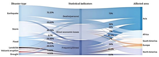
Figure 1.
Sankey map of disaster type, statistical indicators, and affected areas.
The distribution of massive amounts of relief supplies is regarded as one of the core tasks during the post-disaster response phase, which can meet the need of AAs and mitigate the impact of disasters [3]. The effectiveness of the transshipment of massive relief supplies is primarily influenced by two factors: (1) the precision of allocation, which includes the fairness, the priority ranking of demand, and the satisfaction rate [4]; (2) the efficiency of transportation, which involves the availability of transportation resources and the rational selection of transportation modes [5]. Therefore, enhancing the accuracy of allocation and ensuring timely and efficient transportation processes are crucial for optimizing the overall distribution efficiency of massive relief supplies.
Natural disasters often cause extensive damage, and locally stored relief supplies are typically insufficient to meet demand. Moreover, the AAs are usually unable to resume production in the short term. Therefore, it is necessary to transport massive relief supplies through lateral transshipment across inter-regions to meet the basic demand of affected populations [6]. As shown in Figure 2, there is significant interplay between the allocation and transportation of massive relief supplies during lateral transshipment. On the one hand, rational allocation strategies can optimize transportation routes, ensuring that relief supplies are delivered to the AAs rapidly and accurately. The optimal decision regarding the demand for relief supplies includes the type and the volume [7]. On the other hand, the smoothness of the transportation process directly influences the effectiveness of massive relief supplies allocation. This interplay necessitates that, in emergency logistics, the consideration of allocation and transportation must be integrated to achieve efficient distribution of massive relief supplies [8].
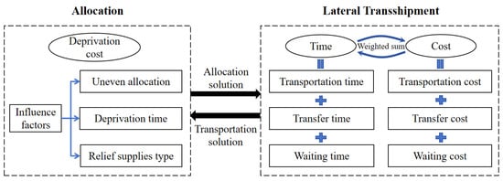
Figure 2.
Relationships between allocation and lateral transshipment.
Humanitarian logistics (HL) has emerged as a popular research area [9], playing a critical role in emergency management [10]. Scholars and practitioners widely agree that alleviating human suffering is the core objective of HL [11,12,13]. Deprivation cost, as an economic indicator that measures human suffering caused by relief supplies shortages, not only provides a means to quantify such suffering but also offers a new perspective for the optimization and performance evaluation of HL. It is influenced by various factors, including the uneven allocation of relief supplies and the deprivation time [14]. Relief supply shortages are critical to rescue efforts [15]. Introducing the deprivation cost concept into the allocation of massive relief supplies enables decision-makers to more comprehensively assess the fairness and efficiency of allocation strategies, thereby meeting the basic demand of AAs while reducing the psychological and social impacts associated with relief supplies shortages. For example, during disaster response, quantifying deprivation cost can optimize the transportation routes and facility location decisions, ensuring that critical resources (e.g., food and medicine) are prioritized for areas with the greatest need.
In addition, selecting appropriate transportation modes is critical for ensuring the rapid delivery of massive relief supplies [3,16]. Under emergency conditions, decision-makers face a dual challenge: adhering to rescue time constraints while minimizing transportation costs [17]. However, in practice, the transportation of massive relief supplies faces the following challenges due to weather and traffic constraints: (1) long transportation distances and the low economic efficiency of a single transportation mode [18]; (2) the transportation chain is lengthy, involving multiple transfer stages, with low transfer efficiency [11]; and (3) the volume of relief supplies allocation is large, while the transportation capacity resources are limited [19]. As an efficient mode of transport, intermodality has a large volume and relatively low transportation cost [20]. Therefore, leveraging the advantages of various transportation modes and formulating scientifically sound intermodality strategies become an effective means to improve quality of rescue services and reduce casualties and property losses.
This paper addresses the massive relief supplies inter-regional lateral transshipment (MRSIRLT) problem, which includes the allocation of massive relief supplies, considering deprivation cost and the inter-regional lateral transshipment by intermodality. The main contributions of this paper are as follows. (1) The paper establishes a two-stage mathematical model. The first stage is the allocation of massive relief supplies, and the second stage is the intermodality route planning. These two stages are interconnected and interactive. (2) This paper makes improvements to help solve the intermodality route planning problem by creating a directed multi-graph and enhancing the attributes of network edges and nodes. Unlike most methods of extending nodes, this strategy reduces the problem scale and accelerates the solution speed. (3) A phased interactive framework incorporating adaptive differential evolution (JADE) and improved adaptive large neighborhood search (IALNS) is proposed, in which JADE is presented to determine the massive relief supplies allocation, and IALNS is used to optimize the intermodality routing. (4) Taking the typhoon disaster in the Bohai Rim region as the background, a case study is constructed to verify the effectiveness and applicability of the model and algorithm. Sensitivity analysis is carried out to provide management insights.
The rest of this paper is organized as follows. Section 2 reviews the related literature. Section 3 is model construction. Section 4 is algorithm design. Section 5 is the experiment study, including sensitivity analysis of key parameters and some management insights. Section 6 concludes and suggests possible future research directions.
2. Literature Review
A considerable number of papers have been published on the problem of allocation and transportation of relief supplies. This paper focuses on the inter-regional lateral transshipment of massive relief supplies, considering intermodality and humanitarian deprivation cost. Therefore, the related papers can be classified into two categories: (1) humanitarian logistics and (2) intermodality.
2.1. Humanitarian Logistics
As the human suffering and economic damages caused by natural disasters continues to rise, HL research is receiving increasing attention [21]. The research framework for HL typically includes three phases: pre-disaster preparedness, post-disaster response, and recovery [22]. Pre-disaster preparedness is aimed at facility location selection and pre-positioning of relief supplies; post-disaster response concentrates on relief supplies allocation, transportation, and the selection of temporary facility locations; the recovery phase involves tasks such as debris clearance, network restoration, and aid distribution.
For the pre-disaster preparedness phase, optimizing the pre-positioning and distribution of relief supplies, as well as the related facilities location and personnel planning, is the key to improving rescue efficiency and response speed. In recent years, many scholars have carried out in-depth research in this field and proposed a variety of optimization models and methods. Che et al. [23] and Torabi et al. [24] proposed a two-stage distributed robust optimization method and a multi-objective mixed-integer linear programming model, respectively, for optimizing pre-positioning and procurement plans for relief supplies. Some scholars have studied how to optimize the pre-positioning and distribution of relief supplies in uncertain environments. They took into account the vulnerability of roads and facilities, and improved the efficiency and effectiveness of disaster response by rationally distributing and pre-positioning relief supplies and optimizing the location of facilities and transportation routes [25,26]. Boonmee et al. [27] proposed optimization models for improving the efficiency and effectiveness of disaster response. These models aim to improve the efficiency of disaster response and reduce the number of untreated casualties by rationally selecting the location of rescue facilities, optimizing the storage and distribution of rescue supplies, and integrating optimal facility location, casualty allocation, and medical staff planning.
This paper focuses on the post-disaster response phase. Despite HL drawing on commercial analytical methods, there are significant differences in various environments between them, leading to limitations in the application of these methods [11]. The core objective of HL is to effectively respond to disasters or emergencies by providing necessary aid and survival essentials to AAs and populations in order to alleviate human suffering and reduce losses [28]. However, existing research often neglects the direct quantification of human suffering or only assesses it through indirect measurements. Thus, it is necessary to find an appropriate method to quantify the suffering of disaster-affected populations during the waiting period for rescue [29,30,31].
To quantify this suffering, Holguín-Veras et al. [11] define the deprivation costs in HL as the human suffering caused by the lack of goods or services related to disasters, and estimate the deprivation cost functions (DCFs) for water using willingness to pay. This concept originates from their discussion on the necessity of reformulating HL models, emphasizing that human suffering should be quantified and incorporated into humanitarian considerations. Holguín-Veras et al. [12] analyzed the differences between commercial logistics and HL, and proposed the use of social costs (sum of logistical costs and deprivation costs) as the preferred objectives for post-disaster HL models, as well as the philosophical significance and complexity of deprivation costs. This method has been widely accepted and is regarded as a novel approach to solve the inappropriate objectives problem in HL [32,33,34].
The concept of deprivation costs has emerged as a significant trend in HL research, with applications spanning various aspects [34,35,36]. Pérez and Holguín-Veras [32] constructed an inventory allocation model for post-disaster HL based on deprivation costs. The contingent valuation (CV) method was successfully employed by Holguín-Veras et al. [14] to estimate DCFs, providing a conceptually effective tool for resource allocation in disaster response and emergency situations. Building on this foundation, Wang et al. [37] proposed the concept of deprivation levels and developed a method using a numerical rating scale (NRS) to estimate deprivation level functions (DLFs) for tents, food, and medicine. They utilized the ordinary least squares estimation algorithm for curve regression, offering new methods and perspectives for studying human suffering in HL. Wang et al. [38] further extended this research by constructing a suffering function using an NRS to describe the perceived suffering costs of disaster victims. Gao et al. [39] constructed an absolute and relative suffering cost function to research the post-earthquake distribution of relief supplies, establishing a two-stage multi-objective model to minimize the average psychological suffering cost and emergency logistics cost of disaster victims. Khodaee et al. [40] investigated the effect of different parameters on total and deprivation costs to minimize total costs while ensuring equitable distribution. Overall, these studies have collectively demonstrated the theoretical and practical validity of deprivation costs in HL, providing a robust framework for understanding and mitigating human suffering in emergency logistics contexts.
2.2. Intermodality
In the post-disaster response phase, the timely and effective transportation of relief supplies to AAs is crucial for saving lives [15]. The deprivation cost associated with the shortage of relief supplies increases exponentially over time [12,14]. Therefore, selecting the appropriate mode of transportation to enhance the transportation efficiency can significantly alleviate the suffering of affected populations [41]. This is essential for accelerating emergency response efforts.
Transportation by a single mode has significant limitations due to the specific nature of relief supplies and the limitations of weather conditions and road traffic [42]. Intermodality has emerged as a more flexible solution, providing alternative options and addressing the complex demands of HL [43]. As a result, intermodality in HL has become a popular area of research that focuses on optimizing transport modes and efficiencies in order to improve the efficiency of emergency response [44,45,46]. However, research on multiple disaster relief supplies under intermodality remains limited [47].
An increasing number of studies have begun to address the limitations of single-commodity, single-mode transportation by researching intermodality solutions. Haghani et al. [48] developed a network flow model with multiple relief supplies and transportation modes aimed at minimizing rescue costs. Ning et al. [49] proposed a two-stage medical supplies combined transportation method based on clustering, constructing a “helicopter-vehicle” transportation network structure. Liu et al. [47] addressed the emergency logistics transportation planning problem by establishing a mixed-integer programming (MIP) model and proposing a two-layer solution method. Weng et al. [50] developed a relief supplies allocation model for public health emergencies under an intermodal network, incorporating psychological pain costs due to shortages of relief supplies. Romero-Mancilla et al. [30] provide a mathematical model of the multi-objective three-level transshipment problem that takes into account the use of a heterogeneous fleet of UAVs and land vehicles. Maghsoudi et al. [18] studied an intermodal model for the distribution of relief supplies, adapting to changes in demand and transportation networks during the disaster response process. Wang et al. [51] constructed a three-layer multi-cycle emergency logistics network of “distribution point-distribution centre-disaster site”, and proposed a new multi-objective optimization model and an improved NSGA-II algorithm considering road damage, multiple transportation modes, and dynamic changes in supply and demand. Zhang et al. [52] constructed a two-layer optimization scheduling model for relief supplies, ensuring rapid delivery within the golden rescue time and guaranteeing the fairness of distribution. These studies exemplify the increasingly important role of intermodality in responding to complex transportation of relief supplies and provide valuable insights and tools to improve the efficiency of humanitarian relief operations.
The main related research is divided into three groups according to different criteria, namely problem characteristics, modeling, and solution approach, as shown in Table 1. Problem characteristics are divided into four categories: deprivation cost, intermodality, multiple types of relief supplies, and massive relief supplies. The second group includes the number of objectives and the model types. Based on the first criterion, papers are divided into two categories: single-objective (SO) and multi-objective (MO). The second criterion includes mixed-integer programming (MIP), mixed-integer linear programming (MILP), and mixed-integer nonlinear programming (MINLP) models. The third group compares solution approach.

Table 1.
Literature review summary.
Through a literature review, the following conclusions can be drawn.
- There have been many studies on the relief supplies distribution, but few studies consider multiple and massive relief supplies at the same time.
- Most studies focus on reducing the cost of or time spent distributing relief supplies and improving fairness, while insufficiently considering the perceived suffering of disaster victims due to resource shortages.
- The transport capacity is often limited in the process of inter-regional lateral transshipment, and the research on the combination of allocation and transportation of massive relief supplies is still relatively lacking.
3. Model Development
3.1. Problem Description
We design a post-disaster logistic network for MRSIRLT problem, as shown in Figure 3. The network is composed of three types of nodes: supply points (SPs), transfer nodes (TNs), and demand points (DPs).
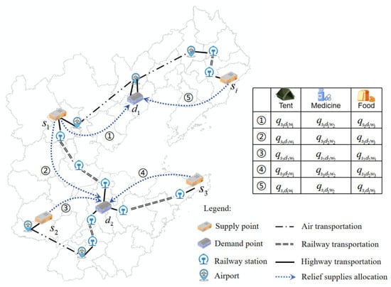
Figure 3.
Logistic network.
- SP: In order to enhance the Government’s disaster relief capacity and reduce the damage caused by disasters to people and property, the State has set up SPs for relief supplies. These SPs, which are pre-positioned with relief supplies, serve primarily to provide emergency relief to victims affected by disasters and to safeguard their basic needs. The location, inventory, and fixed cost of potential SPs are planned by decision makers in advance. SPs are typically distant from disasters, rarely experience disruptions, and can be considered permanent facilities.
- TN: TNs refer to the locations where transfer operations take place between different transportation modes in intermodality, mainly including airports, railway stations, ports, etc. In the context of emergency rescue, due to the relatively slow speed of water transportation, which cannot meet emergency needs, this study only considers airports and railway stations. When transferring at these nodes, there will be certain transfer time and costs, as well as waiting time and costs associated with fixed transportation schedules.
- DP: DPs are the specific locations that require receipt of relief supplies, services, or support in the event of an emergency or disaster. In the post-disaster phase, victims are accommodated in safe locations such as shelters, schools, gymnasiums, and other critical infrastructures. These people require massive relief supplies to survive, including food, water, and tents. Additionally, medical services are crucial for the injured. Due to the unpredictability of disasters, it is difficult to estimate the exact volume of demand. In situations where resources are limited, DPs may need to be prioritized based on urgency and importance.
MRSIRLT is the process of selecting appropriate transportation modes to quickly transport massive relief supplies (food, tents, medicine, etc.) from SPs to DPs under limited space and resources constraints, as shown in Figure 3. Based on actual rescue situations, inter-regional lateral transshipment is divided into two stages, as shown in Figure 4: the first stage is massive relief supplies allocation, and the second stage is intermodality route planning. The decision-makers in the two stages are different; the first stage is the relief supplies allocator, and the second stage is the route planner. The decision content is different; the first stage decision-makers need to determine the relief supplies type and volume between different SPs and DPs based on demand and deprivation time. That is, it is assumed that there are types of relief supplies, , stored in , with demand points at , and decisions are made on the amount of relief supplies allocated from to . The second stage decision-maker decides on the intermodality plan from SP to DP. As shown in Figure 3, the transportation mode from to is highway, railway, highway. The decision objectives vary: the first stage aims to minimize the deprivation cost, while the second stage emphasizes minimizing the weighted cost of transportation time and costs. The two stages are interrelated and mutually constrained; the allocation volume obtained in the first stage is passed to the second stage for route planning, and the transportation time (travel time + transfer time + waiting time ) obtained in the second stage is fed back to the first stage as the basis for SP selection, and only SPs whose transportation time is within the time threshold can be allocated.
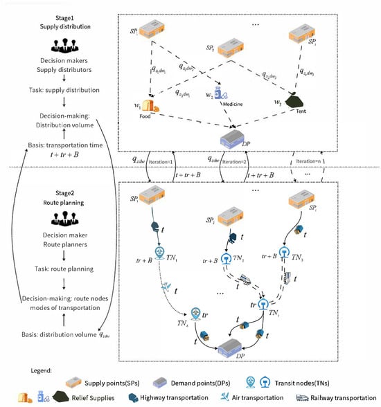
Figure 4.
Two-stage schematic.
In the first stage, we assume that the relief supplies are indivisible. This ensures the integrity of the relief supplies, and certain relief supplies (such as tents and medical equipment) cannot be used in a randomly divided manner and must be allocated in complete units. At the same time, this assumption simplifies the allocation process, makes the allocation decision clearer and more efficient, and improves the efficiency of allocating relief supplies. From the point of view of actual demand, indivisible relief supplies are more in line with the needs of the rescue site, and can better support emergency rescue. In the second stage, it is essential to assume that the fixed unit cost is related only to the quantity of relief supplies and the mode and time of transportation. This assumption makes the model more concise and easier to analyze and solve. The quantity of relief supplies determines the scale of transportation and resource requirements, the mode of transportation determines the cost structure and efficiency of transportation, and the time of transportation affects the accumulation and timeliness of transportation costs. Through this assumption, the complex transportation cost factors can be effectively integrated, avoiding the introduction of too many variables, which could make the model too complex and difficult to solve.
3.2. Model Formulation
Model assumptions
- Relief supplies are indivisible during transportation.
- The transfer of transportation modes only occurs at the TNs, and can only take place at most once at each TN.
- The transportation costs between nodes are only related to the volume of relief supplies, the transportation modes, and time, which are independent of the departure time at the nodes.
- The transfer cost at a TN is only related to the transfer mode and the node itself.
- The cost of waiting at a TN is related only to the volume of relief supplies and the waiting time.
3.2.1. Stage1 Model Formulation
The significance of the symbols involved in the stage 1 model is as shown in Table 2.
Table 2.
Symbol description of stage 1 model.
Objective function
In stage 1, we minimize the deprivation cost caused by the deprivation number of relief supplies; denotes the sum of the deprivation costs.
Constraint (2) ensures that the number of relief supplies transported from SPs cannot exceed their inventory. Constraint (3) guarantees that the ratio of the number of relief supplies actually delivered to DPs to the quantity demanded will not be less than the minimum satisfaction rate for that relief supply. Referring to Wang et al. [38], Constraint (4) denotes the deprivation cost function incurred by the lack of a certain type of relief supply at DPs, where are the parameters of the deprivation cost function. Constraint (5) denotes that the shortage number of relief supplies delivered to DPs. Constraint (6) defines the non-negative constraints of decision variables.
The deprivation cost in the objective function of the above model is a power function, so it is a nonlinear integer programming problem. Traditional optimization methods, such as branch-and-bound and cut-plane methods, are not effective in solving the problem for large-scale cases. Therefore, we specifically design differential evolutionary algorithms for solving this model in the next section.
3.2.2. Stage2 Model Formulation
The significance of the symbols involved in the stage 2 model is as shown in Table 3.
Table 3.
Symbol description of stage 2 model.
Objective function
In Stage 2, we aim to optimize the cost and time. Objective function (7) minimizes the total time, including the transport time from SPs to DPs, transfer time from one transportation mode to another at the TN, and waiting time due to the transportation schedules; denotes the sum of the total time. Objective function (8) minimizes the total cost, including the transportation cost, transfer cost, and waiting cost at the TN; denotes the sum of the total costs.
Constraint (9) represents the path selection flow balance. Constraint (10) indicates that the actual arrival of the relief supplies at DPs is earlier than the latest permitted arrival time. Constraint (11) denotes the waiting time at the node. Constraint (12) ensures that two adjacent nodes choose only one transportation mode. Constraint (13) indicates that the volume of relief supplies transported on a road section is not greater than its transport capacity. Constraint (14) indicates that the volume of relief supplies transfer at the TN is not greater than its maximum transfer capacity. Constraint (15) guarantees transport continuity, i.e., if at node the transportation mode is transferred from to , then the transportation mode chosen at node is , and the transportation mode arriving at node is . Constraint (16) ensures that there can be no more than one transfer at the TN. Constraint (17) indicates that the volume of relief supplies departing from each node cannot exceed the volume capacity limit of the transport vehicles at that node. Constraint (18) states that the weight of relief supplies departing from each node cannot exceed the payload limit of the transport vehicles at that node. Constraints (19) and (20) define the 0–1 variable constraints; Constraint (21) defines the non-negative constraints.
4. Solution Approach
In this paper, a phased interactive JADE and IALNS optimization algorithm is designed to solve the model. The JADE algorithm solves the first-stage massive relief supplies allocation problem to determine the types and volume of relief supplies to be distributed from SPs to DPs. The obtained massive relief supplies allocation relationship is then further used as an input parameter for transportation route planning in the inner algorithm. In the second stage, the IALNS algorithm is employed to deal with the intermodality issue to optimize transportation routes from SPs to DPs. Before the second stage begins, we introduce a feasibility checking subroutine which verifies the network feasibility of the first stage results. If the result is not feasible, the subroutine will adjust the road network accessibility. In addition, after each iteration of the second stage, we introduce a double validation loop that ensures that the current solution satisfies the network feasibility condition. If the current solution is not feasible, the loop will adjust the solution until a feasible solution is found. Then, the allocation and transportation solutions are passed into the outer algorithm to select the optimal solution based on the fitness function and determine whether the number of iterations in the outer layer are satisfactory. If it is not satisfied, the obtained transportation solution is passed into the outer layer algorithm for selecting SP, and the iterative process is repeated and updated. If it is satisfied, the optimal solution is output. The algorithmic framework diagram is shown in Figure 5.

Figure 5.
Algorithm framework diagram.
4.1. JADE Algorithm
The model constructed in the first stage is a typical real-number planning model for material allocation, which has been proven to be an NP-hard problem and cannot be solved in polynomial time. Therefore, in this paper, the model is solved by designing a heuristic algorithm, the JADE algorithm. The differential evolutionary (DE) algorithm is a population-based adaptive global optimization algorithm with strong robustness and global optimization seeking ability that is mainly used to solve real number optimization problems. In JADE, the two key parameters of DE, scaling factor (F) and crossover probability (CR), are dynamically adjusted using adaptive mechanisms. This allows the algorithm to automatically tune itself to different optimization problems and stages of the search process. The process is as follows.
4.1.1. Encoding & Decoding
A three-dimensional matrix was constructed to represent the individuals in the population. The dimensions of this matrix are the number of SPs multiplied by the number of relief supply types, and further multiplied by the number of DPs. The values within the matrix indicate the volume of a specific relief supply allocated by a particular SP to a specific DP. The allocation volume range is defined based on the demand at the DPs, the inventory at the SPs, and the number of SPs within the time threshold, which generates the upper and lower bounds for the JADE algorithm. Given that the encoding is in real numbers, the values are processed with ceiling functions to ensure integer results. The formula for the upper bound is shown in Equation (22), and the formula for the lower bound is shown in Equation (23).
where represents the demand for relief supply at the DP , , represents the total number of SPs, represents the number of SPs exceeding the transportation time threshold, and represents the number of relief supply stored at SP , .
4.1.2. Calculate Fitness Value
Based on the massive relief supplies allocation from SPs to DPs, calculate the deprivation cost for each DP. For the amount of relief supplies that exceed the demand at DPs, surpass the inventory at SPs, and fail to meet the requirements, penalty coefficients are applied to penalize accordingly, resulting in the fitness value.
4.1.3. Adaptive Parameter Strategy
For each generation , the crossover probability of each individual is independently generated according to a normal distribution of mean and standard deviation , and then truncated to [0, 1]. Denote as the set of all successful crossover probabilities at generation . The mean is initialized to be 0.5 and the updated at the end of each generation as Equation (25).
where is a positive constant between 0 and 1, and is the usual arithmetic mean.
Similarly, at each generation , the mutation factor of each individual is independently generated according to a Cauchy distribution with location parameter and scale parameter 0.1, and then truncated to be 1 if , regenerated if . Denote as the set of all successful mutation factors in generation . The location parameter of the Cauchy distribution is initialized to be 0.5, and then updated at the end of each generation as Equation (27).
where is the Lehmer mean
4.1.4. Mutation
In order to extend the diversity of population and avoid computation overhead, the inferior solutions saved in the external archive is considered in the DE/current-to-pbest/1 with external archive strategy. In this strategy, a mutation vector is generated as follows:
where , and are selected from P, while is randomly chosen from the union, P ∪ A, in which A is the set of archived inferior solutions and P is the current population.
4.1.5. Crossover
The crossover operation is performed between the individual produced by the mutation and the individual in the population to obtain the following test individuals:
where , is the dimension of the decision variable, is the crossover factor.
4.1.6. Selection
The DE algorithm is based on a greedy selection between the test vector and the individuals of the original population. The principle of selection is that the individual with the better fitness value enters the next generation, which is expressed in the following equation:
Of these, is the fitness function.
4.1.7. Termination Condition
Terminate the iteration when the number of iterations exceeds the maximum number of iterations.
4.2. IALNS Algorithm
Second-stage intermodality route planning mainly involves transportation mode selection and route optimization, which is a typical combinatorial optimization problem that has been proved to be an NP-hard problem. Therefore, in this paper, a heuristic algorithm, the IALNS algorithm, is designed for solving the problem.
The core idea of an ALNS algorithm is to destroy the solution, repair the solution, dynamically adjust the weights, and select. By designing multiple sets of destroy and repair operators, the solution space search range is expanded, and the current solution is improved. In each iteration, based on previous performance, the selection and weighting adjustment of various destruction and repair operators are conducted, using efficient combination methods to enhance the algorithm’s optimization capability, thereby finding the optimal solution. The process is as follows.
4.2.1. Initial Solution
Depending on the different problems, various heuristic rules can be employed to generate feasible solutions. For the route planning in this study, Dijkstra’s algorithm is used to generate a sequence of paths consisting of node numbers as the initial feasible solution. The coding diagram is shown in Figure 6.
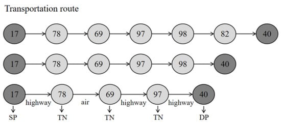
Figure 6.
Coding diagram.
4.2.2. Destroy
The main methods for destroying solutions include random removal and worst-case removal, among others. Among them, random removal involves deleting any node within the current path solution, whereas worst-case removal entails deleting the road segment with a higher fitness value within the current path solution, as shown in Figure 7. Destroy and then repair, with this step yielding a destroyed solution and a list of removed nodes.
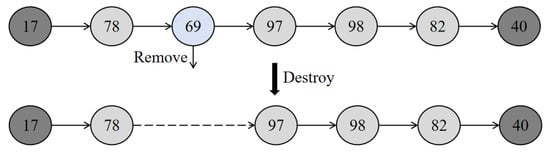
Figure 7.
Schematic diagram of destroy.
4.2.3. Repair
The methods for repairing the solution include random insertion and greedy insertion. Random insertion involves randomly inserting a set of feasible paths between the destroyed nodes; greedy insertion, on the other hand, selects the set of nodes with the smallest fitness value among the feasible paths for insertion between the destroyed nodes. The goal of the repair operation is to connect the destroyed segments by inserting other feasible nodes, thereby obtaining a complete new solution set, as shown in Figure 8.
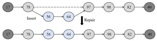
Figure 8.
Schematic diagram of repair.
4.2.4. Dynamic Adjustment of Weights and Selection (Adaptive Process)
During iteration, the algorithm selects and adjusts the destroy and repair operators based on operator weights and a roulette wheel method.
- Weights update
The weights of the operators are updated according to the following formula:
Of these, is the operator weight, is the operator score, is the number of times the operator has been used, and is the weight update coefficient.
At the beginning, all operators have the same weights and scores. During each iteration, scores are assigned based on the performance of each operator, with higher scores indicating better performance. In the search process, if only the superior solution is selected, it is easy to fall into the local optimum. In order to avoid this situation, ALNS usually uses the simulated annealing algorithm metropolis criterion, which accepts inferior solutions under a certain probability.
- 2.
- Roulette selection
After obtaining the new weights, the algorithm selects the operators based on the roulette method so that the probability of an operator being selected is proportional to its weight performance.
4.2.5. Fitness Value Calculation
Calculate the time and cost of each transportation route, including transportation time, transfer time, and waiting time, with corresponding costs for transportation, transfer, and waiting. The time and cost are then weighted and summed, with the weight coefficients adjustable according to the decision-maker’s preferences.
4.3. Intermodality Network Improvement Strategies
In previous studies, the treatment of intermodality networks often involved decomposing nodes, then splitting a single node into departure and arrival nodes to expand the network [53]. However, using this method increases complexity. Taking a road network with seven nodes as an example, with the network including one SP: A, one DP: G, and five TNs: B, C, D, E, F, with eight edges connecting these nodes. Different transportation modes can be used between nodes for transportation, as shown in the actual highway-rail-air network in Figure 9.
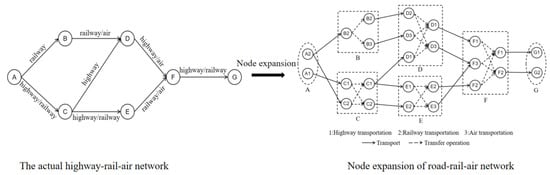
Figure 9.
Transportation network diagram after node expansion.
Considering that the mode of transportation when relief supplies enter a node may differ from the mode when they leave that node, meaning that a transfer operation between different transportation modes occurs at that point, the nodes in the intermodality network are modified as follows. Each node is split into departure and arrival nodes. If there are transportation modes that can transport relief supplies to node at node , and transportation modes available to choose from at node , then node in the intermodality network is split into arrival nodes and m departure nodes. By applying this treatment to each node, the resulting intermodality network path diagram after node splitting is shown in Figure 9. The expanded road network has a total of 25 nodes and 36 edges.
This paper makes improvements to address this issue by creating a directed multi-graph and enhancing the attributes of network edges and nodes. It allows for multiple edges between the same pair of nodes. By flexibly adding or modifying the attributes of nodes and edges without increasing their number, it adapts to different modes of transportation and requirements, enabling more complex network relationships and attribute management. This approach avoids unnecessary replication of nodes and edges, is more efficient, and maintains the manageability and scalability of the network. The decomposed intermodality network diagram is shown in Figure 10. For example, if C-E can be connected to railway and highway, air is not available; in that case the relief supplies can be transferred to railway or highway at point C, and then transported to point E, but cannot be converted to air transport.
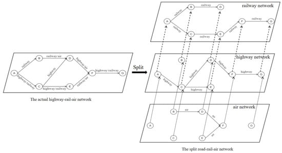
Figure 10.
Intermodality network split diagram.
5. Case Study
In this section, a case is designed to evaluate the two-stage model developed in this paper as well as the solution algorithm. We use Python 3.8 as the development environment. The tests were run on an Intel (R) Core (TM) i5-1240P 2.40 GHz laptop with 16 GB RAM.
5.1. Case Study Description
As a natural disaster, typhoons cause significant damage. In the past 10 years, China has experienced an average of about 10 typhoons making landfall each year, resulting in substantial economic losses and casualties [54]. The achievement of safe, rapid, and economical transportation of massive relief supplies is crucial to the economic and social stability of AAs. Because of its special geographical location and climatic conditions, the Bohai Rim region is frequently affected by typhoons and other natural disasters, which bring serious challenges to the lives of local residents and economic development. According to the analysis of the June–September typhoon optimal path dataset and day-by-day precipitation data from national meteorological observatories from 1961–2023, an average of one to two typhoons affect the Bohai Rim region each year, with August and September being the most frequent months. Second, the Bohai Rim region has a high population density, and when a typhoon disaster occurs, the affected population is huge, and there is an urgent need for rescue and relief supplies distribution. In addition, the region has a higher level of economic development, and the impact of typhoon disasters on the economy is more significant. In summary, typhoon disasters in this region are special and complex and require in-depth research and analysis to improve disaster prevention and mitigation capabilities. In view of this background, this paper chooses typhoon disasters in the Bohai Rim region as the background for the case study.
Taking the 2019 “Lekima” typhoon as the background and in line with research requirements, this paper selects five provinces and municipalities in the Bohai Rim region, including Hebei, Shandong, Liaoning, Beijing, and Tianjin, as the research subjects. We choose 22 provincial and municipal supply reserve warehouses in Shenyang, Tianjin, Beijing, etc., as SPs and randomly generate DPs in 42 cities within the region. The case considers 22 SPs, 81 TNs, three transportation modes, three types of relief supplies, and 42 DPs. Figure 11 shows the distribution of SPs, DPs, and TNs, and the specific information is in Table A1. The numbers in the figure are node numbers; purple is the SP, red is the DP, green is the railway station, and blue is the airport. Since highway transport is more flexible, it can stop at any point along the route, including nodes where railway stations and airports are located. Therefore, there are no transfer points for highway transport on the network, and highway transport can transfer at airports or railway stations, which also simplifies the network to a certain extent. Since some data cannot be accurately obtained, we adopt a method that combines real data with partially simulated data to set parameter values. Simulation data can demonstrate the effectiveness of the model and algorithm without essentially impacting the conclusions. At the same time, the setting of simulation data is based on relevant data under normal social conditions.
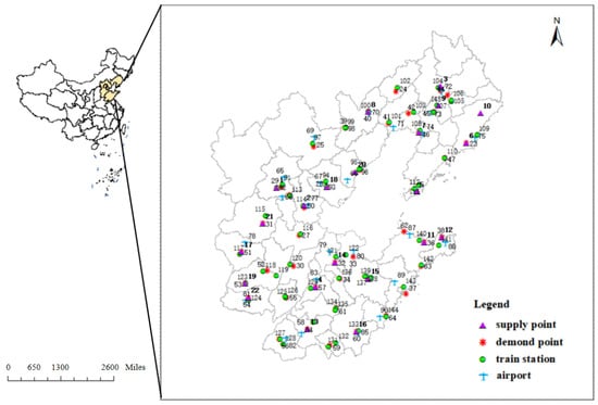
Figure 11.
Map of SPs, TNs, and DPs.
Referring to the research data of Wang et al. [37], nonlinear regression methods were applied to analyze the data of three types of relief supplies: tents, food, and medicine, for the fitting of deprivation cost functions [38]. The least squares method was used to perform a significance test on the fitting functions. The results indicate that the power function exhibits the best fitting effect. At a confidence level of 95%, the results of the nonlinear regression analysis for different types of relief supplies can pass the significance test. At this time, the deprivation cost functions are as follows.
Of these, represents the type of relief supply; represents the deprivation time; represents the deprivation cost; and and are parameters; specific values are shown in Table 4.
Table 4.
Deprivation cost function parameter data.
Different levels of SPs have varying capacities. The input parameters for SPs can be found in Table A1. The distances between various nodes in the network were obtained through Baidu Maps, while the air transportation times were sourced from the 12,306 China Air Timetable. The transportation times for railways and highways were calculated based on the distances and speeds involved. The “14th Five-Year Plan” for the national emergency management system proposes that the time for effectively assisting people affected by disasters to meet their basic living needs should be reduced to within 10 h [55]. Therefore, this paper sets the transportation time threshold to 10 h, meaning that only SPs within a 10 h travel time from the DPs can allocate relief supplies to those DPs. The costs associated with different transportation modes vary. This paper considers that the unit transportation cost is only related to the transportation mode and does not take into account special circumstances (such as changes in fuel prices, weather factors, etc.). The unit transportation cost (CNY) for different modes is set as follows: highway (760), aviation (3000), and railway (500). The transportation capacity of each road segment differs under different transportation modes, with the number of transport vehicles set at 100 for highways, 20 for railways, and five for air.
At the TNs, different modes of transportation can be transferred, which requires a certain amount of time and cost, and there are limitations on the transfer capacity. This paper assumes that no transfers occur between the same transportation mode; that is, if the same mode is used for both entering and leaving a node, no transfer operation is performed. The unit transfer costs (CNY) and transfer times (hours) between different transportation modes are shown in Table 5. Additionally, it is assumed that the costs and time consumed for transferring between two transportation modes are consistent. The transfer capacities (tons) are set as follows: airport (12,000) and railway station (2000).
Table 5.
Unit transfer costs (CNY)/transfer times (h) between different transportation modes.
In the actual transportation processes, railway and air transportation, due to their higher maintenance and operational costs, are much more complex to schedule than highway transportation. Therefore, they typically have fixed departure times, which we refer to as fixed transportation schedules [56]. If the arrival time at a TN is earlier than the departure time of the transportation mode at that node, there will be waiting; if it is later, one must wait for the next available departure. In view of the emergency context, the frequency interval of rail and air transportation at each node is set at 2 h and 4 h respectively, and it is assumed that the unit waiting cost due to waiting for departure times is 200 (CNY/()).
The demand for relief supplies at each DP is estimated based on the population, with proportions derived as follows: food at 15%, medicine and tents at 10%. Specific information is provided in Table A1. This method reflects the fairness of demand, ensuring that different demand points receive relatively balanced allocation of relief supplies. At the same time, it simplifies the demand forecasting process and quickly estimates the approximate demand at each DP, providing a clear reference basis for decision makers and facilitating rapid and rational allocation decisions in emergency scenarios. In addition, the method is highly adaptable and can be applied to different scales and types of emergency events; it can also adjust the demand forecast in time according to the population changes, facilitating data acquisition and updating. Randomly generate priority levels for both the DPs and the various types of relief supplies, with higher numerical values indicating higher priorities. The product of these two priorities represents the priority of that particular relief supply at the corresponding DP. The weights and volumes of various relief supplies are shown in Table 6, while the load and volume of the transportation vehicles are shown in Table 7.
Table 6.
The weight and volume of different supplies.
Table 7.
Unit load and volume of different transportation modes.
5.2. Simulation Results
To better illustrate the allocation and transportation plans for massive relief supplies in disasters of different scales, we randomly generate three scenarios with varying sizes (large: three DPs, medium: two DPs, small: one DP), and obtain the optimal solutions. To verify the stability of the model and algorithm, we run each of the three scenarios 25 times.
The relief supplies satisfaction rate is shown in Table 8. In the small scenario, the satisfaction rates of the three relief supplies types are all above 98%. This indicates that the supply meets the demand, demonstrating the superior performance of the algorithm and its high fairness. The satisfaction rates of relief supplies in the medium scenario, all above 95%, and in the large scenario, above 90%. The average value is close to the median, indicating a relatively uniform data distribution. The overall satisfaction rates for all types of relief supplies in the three scenarios are relatively high, with medians all above 92% and the maximum–minimum gap all less than 3%, indicating a high level of fairness in the distribution outcomes. Under the three scenarios, the satisfaction rate trends of different relief supplies are shown in Figure 12. Overall, as the scale of the scenario increases, the satisfaction rate with relief supplies tends to decrease, with increased fluctuations and reduced stability. The small scenario is more likely to achieve a high satisfaction rate, which may be due to the increased number of DPs in larger scenarios, involving more complexity and uncertainty. Furthermore, within the same scenario, the average satisfaction rates and medians are relatively close across different relief supplies, indicating that the central tendency of satisfaction rates remains relatively stable across multiple runs.
Table 8.
The satisfaction rates of relief supplies in three scenarios.
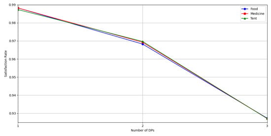
Figure 12.
Average satisfaction rate of relief supplies in different scenarios.
The convergence diagram of deprivation cost under three scenarios is shown in Figure 13. The deprivation cost decreases rapidly during the first 200 iterations, indicating that the algorithm has a fast convergence rate in its initial stage and is capable of quickly identifying a relatively optimal solution. After 200 iterations, the rate of decline in deprivation cost significantly slows down and eventually stabilizes around 270 iterations without significant fluctuations. This demonstrates that the algorithm has good convergence stability, being able to maintain stability after finding a relatively optimal solution. Moreover, as can be seen from the trend, the deprivation cost increases as the scale of DPs increases.
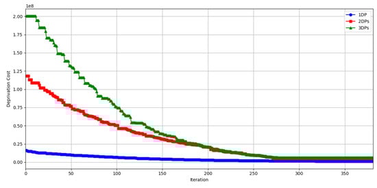
Figure 13.
Deprivation cost convergence diagram.
The running time and memory consumption of different iterations in the three scenarios are shown in Table 9. The data in the table is the average value of the 25 iterations.
Table 9.
Runtime and memory consumption.
The massive relief supplies allocation results for the small scenario are shown in Figure 14, where the table represents the allocation plan and transportation routes for three relief supplies. ‘Route’ refers to the transportation route; for example, 20-(1)-68-(3)-78-(1)-31 indicates that relief supplies are transported from SP 20 to DP 31, includes highway transport from SP 20 to Airport 68, followed by air transport to Airport 78, and finally highway transport to DP 31 (1 represents highway transportation, 2 represents railway transportation, and 3 represents air transportation). ‘Volume’ denotes the volume of relief supplies distributed, for example, 115,871 units of medicines are transported from SP 20 to DP 31.
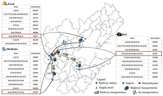
Figure 14.
Transportation route results.
5.3. Sensitivity Analysis
After the occurrence of a disaster, there is mixed uncertainty in the allocation and transportation of massive relief supplies, such as the weights , , for time (denoted as ) and cost (denoted as ), as well as the time threshold . Therefore, by analyzing the time threshold, transfer time, satisfaction rate, and the decision-maker’s preferences, the system adjusts the parameter values to assess their impact on the model’s performance.
5.3.1. Increasing Time Weight Coefficient and Minimum Satisfaction Rate
The time threshold is set to 10 h, under conditions of minimum relief supplies satisfaction rates of 85%, 90%, and 95%, respectively, with time weights of 0.5, 0.6, 0.7, 0.8, 0.9 are generated, with corresponding cost weights of 0.5, 0.4, 0.3, 0.2, 0.1, resulting in a total of 15 scenarios. Solve each scenario to obtain the time and cost spent. As shown in Figure 15, under the 85% satisfaction rate, the lowest time corresponds to the weights of 0.9/0.1, at which point the cost is not the lowest; the lowest cost corresponds to the weights of 0.5/0.5, at which point the time is relatively high. This indicates that it is not possible to simultaneously improve one objective without compromising the other; therefore, the time weights and cost weights form a Pareto solution. The combinations of 0.9/0.1 and 0.5/0.5 are solutions on the Pareto frontier. Decision-makers can adjust the weights according to their priorities to meet their requirements. The combination of 0.67/0.33 represents the crossover point, indicating that an equilibrium state is achieved, where the objective function attains its optimal value. Under the 90% satisfaction rate, the equilibrium point is around 0.69/0.31, and under the 95% satisfaction rate, the equilibrium point is 0.72/0.28. Therefore, to achieve a higher satisfaction rate, the time weight can be set within the range of [0.67, 0.72].
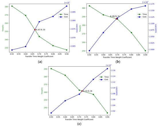
Figure 15.
Time, cost sensitivity to time weights and minimum satisfaction rate. (a) Minimum satisfaction rate: 85%; (b) Minimum satisfaction rate: 90%; (c) Minimum satisfaction rate: 95%.
5.3.2. Decreasing the Time Threshold and Transfer Time
The time threshold affects the selection of SPs in the first stage, which in turn affects the allocation solution. Therefore, this paper generates five scenarios with time thresholds of 10, 9, 8, 7, and 6 h for small-scale scenarios to conduct a sensitivity analysis. The weights for time and cost are set to 0.7/0.3, respectively, to obtain the actual satisfaction rate, time, and cost for each scenario. The relief supplies satisfaction rate under different time thresholds is shown in Figure 16. As the time threshold decreases, the number of assignable SPs diminishes, resulting the demand satisfaction rate for the three relief supplies declines. Therefore, to reduce the time threshold while meeting demand, it is necessary to increase the number of SPs and improve construction density, which will lead to an increase in construction costs. Hence, a 10-h range ensures a higher relief supplies satisfaction rate for DPs while minimizing construction costs. Additionally, there are differences in the variation curves of different relief supplies. When the time threshold is reduced from 10 h to 8 h, the satisfaction rate drops from over 95% to around 80%, especially for medicine, which fall below 80%. This indicates that more urgent relief supply require enhanced transportation efficiency.
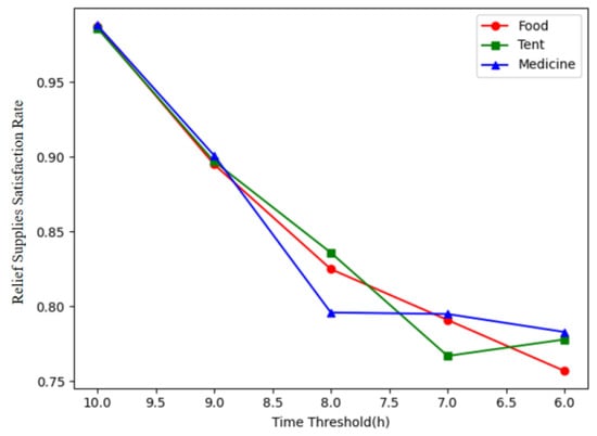
Figure 16.
Satisfaction rate sensitivity to time threshold.
Transfer time is one of the important factors affecting the total transportation time. The length of loading and unloading time directly affects the residence time of massive relief supplies at the TN, thus affecting the efficiency of the entire transportation process. A coefficient is added to the transfer time to control its downward trend, with six scenarios set for the transfer time coefficient of 1, 0.9, 0.8, 0.7, 0.6, and 0.5. The trends of time and cost for each scenario are shown in Figure 17. When the transfer time is reduced by 50%, the total time decreases by 16%. Since the transfer cost set in this paper is only related to the number of transfers and not to the transfer time, the cost trend remains relatively stable. Therefore, optimizing the transfer time can significantly enhance the efficiency of massive relief supplies transportation.
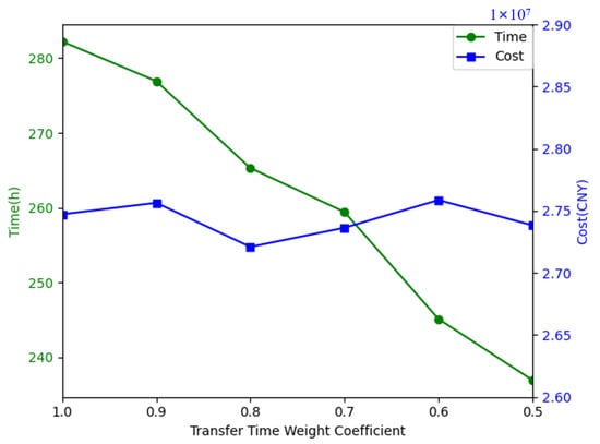
Figure 17.
Time, cost sensitivity to transfer time coefficient.
Through the case study, the following conclusions can be drawn.
- The overall satisfaction rate for all types of relief supplies in different scale scenarios is high, which indicates that the supply meets the demand and proves the superior performance and high fairness of the algorithm.
- To achieve a higher satisfaction rate, the time weights can be set in the range of [0.67, 0.72].
- A sensitivity analysis of the time thresholds shows that the more urgent the relief supplies, the more efficient the transportation needs to be.
- Transfer time had a significant effect on total time, which was reduced by 16% when transfer time was reduced by 50%.
6. Discussion
The results of this study are of great significance to the Bohai Rim region, which is often affected by typhoons and other natural disasters. Optimizing the relief supplies inter-regional lateral transshipment system through the two-stage model established in this paper can improve the emergency response capability of the region and ensure that relief supplies are delivered to the AAs in a timely manner. The model can determine the most efficient routes and transportation modes for delivering relief supplies through intermodality, which can help to shorten transportation time and reduce transportation costs. This is particularly important in disaster relief situations where time is of the essence. By reducing transportation time and optimizing resource allocation, we can save hundreds of thousands of RMB in logistics costs. The model is not limited to typhoon situations. It can also be applied to other natural disasters such as earthquakes and floods. For example, in an earthquake situation, the model can help determine the safest and fastest route. In a flood situation, it can optimize the distribution of water and food to the AAs. To further illustrate our findings, we explored the relationship between the weighted range of time and cost and the actual time and cost consumed, showing that a reasonable setting of the weighting coefficients of time and cost can effectively save time and cost.
This study is also subject to some limitations. Firstly, when studying deprivation costs, cultural differences between countries and regions must be fully considered. These differences may lead to significant variations in deprivation cost parameters. Therefore, it is recommended to conduct investigations based on the cultural backgrounds and actual situations of different provinces and cities, and establish differentiated parameters to ensure the accuracy and applicability of the research. However, this is not the focus of this paper, and future research can further explore this issue. Additionally, due to data limitations, this paper only considered the number of transshipment in calculating transfer time and cost, without adequately considering differences in transfer volume and transfer nodes. This limitation may affect the comprehensiveness of the research results. Therefore, in future research, it is suggested to incorporate transfer volume and transfer nodes to more accurately reflect the actual situation.
7. Recommendation
The primary outcomes of the case study are the results of numerical experiments, which provide numerous recommendations for the inter-regional lateral transshipment of massive relief supplies. It should be noted that these results are not universal and upon the parameter settings. By focusing on minimizing deprivation costs as well as the distribution time and costs, this study can assist decision-makers in enhancing the efficiency and effectiveness of disaster response actions. The model takes into account three types of relief supplies, establishes a transportation network including transfer nodes, and completes the inter-regional lateral transshipment of massive relief supplies under the condition of determined demand. The following recommendations are proposed:
- Transshipment is the key link of massive relief supplies collection and distribution. By optimizing the collection and distribution process, transshipment efficiency can be significantly improved, and the transfer time can be shortened. Measures can be taken: (1) Planning the location of TNs reasonably to ensure they are close to major traffic arteries and areas with high demand density. (2) Increasing the use of modern transfer facilities to shorten loading and unloading times. (3) Improving the skill levels and emergency handling capabilities of operational staff to ensure the smooth progress of the transfer process.
- In the state of emergency response, the factor of time is crucial, while the economic aspect is relatively secondary. The optimal time weight in this paper falls within the range of [0.67, 0.72]. Such weight distribution helps to ensure that rescue operations respond swiftly, meeting the strict time requirements of emergency situations, while reducing transportation costs.
8. Conclusions
Based on review of literatures, this paper conducts a preliminary study on the inter-regional lateral transshipment of massive relief supplies under the background of natural disasters. The main contents are as follows:
Construct a two-stage AIOM for the MRSIRLT problem. With the objective of minimizing deprivation costs, a allocation model for multiple and massive relief supplies from SPs to DPs is established. Considering fixed transportation schedules and utilizing network models from graph theory, a intermodality routing optimization model is developed with the goal of minimizing the weighted costs of transportation expenses and time. Decision-makers can adjust weights according to demand, which allows for a better balance between transportation costs and time compared to general single-objective models. Design a phased interactive JADE and IALNS to solve the two-stage model. Handling intermodality networks by creating directed multi-graph and enhancing the attributes of network edges and nodes avoids unnecessary node and edge replication, is more efficient, and maintains the manageability and scalability of the network. Taking typhoon disaster around Bohai Rim region as the background, the effectiveness of the model and algorithm is verified by solving examples of different scales. The results show that the relief supplies satisfaction rate is above 98% in the small scenario, and above 92% in the large scenario, meeting the demand. With the increase of demand scales, the satisfaction rate shows a downward trend. We also performed a sensitivity analysis to observe the effects of time thresholds, transfer time and time weights on the objectives. Some important management insights are derived as follows. Firstly, under the background of multi-regional disasters, inter-regional dispatch is worthy of in-depth research and discussion. Secondly, improving transfer efficiency and shortening transfer time can effectively improve the of intermodality efficiency. Lastly, in order to realize the dual optimization of time and cost, when the two are weighted, the time weight is preferably [0.67, 0.72].
Author Contributions
Conceptualization, S.L. and N.Z.; Data curation, S.L. and N.Z.; Formal analysis, N.Z.; Funding acquisition, S.L. and N.Z.; Investigation, N.Z.; Methodology, S.L. and N.Z.; Project administration, S.L.; Resources, S.L.; Software, N.Z.; Supervision, S.L. and J.Q.; Validation, N.Z.; Visualization, N.Z. and J.Q.; Writing—original draft, N.Z.; Writing—review & editing, S.L. and J.Q. All authors have read and agreed to the published version of the manuscript.
Funding
This research was funded by National Natural Science Foundation of China, grant number 72474231 and 72074073, and Natural Science Foundation of Hunan Province, grant number 2024JJ5450.
Data Availability Statement
The datasets generated during and analyzed during the current study are available from the corresponding author upon reasonable request.
Conflicts of Interest
The authors declare no conflicts of interest.
Appendix A
Table A1 is the node datas.
Table A1.
Node information.
Table A1.
Node information.
| Node Number | Node Name | Node Type | Node Longitude | Nodal Latitude | Stock/Demand | ||
|---|---|---|---|---|---|---|---|
| Food | Medicine | Tent | |||||
| 1 | Beijing | 1 | 116.258225 | 39.842652 | 329521 | 219681 | 219681 |
| 2 | Tianjin | 1 | 117.216107 | 39.173165 | 344961 | 229974 | 229974 |
| 3 | Shenyang | 1 | 123.507803 | 41.828794 | 268765 | 179177 | 179177 |
| 4 | Jinan | 1 | 117.126974 | 36.654238 | 199025 | 132683 | 132683 |
| 5 | Dalian | 1 | 121.615304 | 38.918953 | 141720 | 94480 | 94480 |
| 6 | Dandong | 1 | 123.9351155 | 39.98516852 | 52753 | 35169 | 35169 |
| 7 | Yingkou | 1 | 122.224651 | 40.632894 | 56780 | 37854 | 37854 |
| 8 | Chaoyang | 1 | 120.447148 | 41.581549 | 81905 | 54604 | 54604 |
| 9 | Liaoyang | 1 | 123.239342 | 41.275463 | 45840 | 30560 | 30560 |
| 10 | Kuandian | 1 | 124.763407 | 40.738867 | 9743 | 6496 | 6496 |
| 11 | Yantai | 1 | 121.4869018 | 37.37626301 | 119602 | 79735 | 79735 |
| 12 | Weihai | 1 | 122.178425 | 37.41224732 | 60383 | 40255 | 40255 |
| 13 | Jining | 1 | 116.594764 | 35.422059 | 202939 | 135293 | 135293 |
| 14 | Binzhou | 1 | 118.0142527 | 37.29223196 | 103388 | 68925 | 68925 |
| 15 | Weifang | 1 | 119.1492527 | 36.62869295 | 189131 | 126087 | 126087 |
| 16 | Linyi | 1 | 118.360087 | 35.114924 | 308934 | 205956 | 205956 |
| 17 | Shijiazhuang | 1 | 114.523254 | 38.050131 | 191818 | 127879 | 127879 |
| 18 | Tangshan | 1 | 118.2208226 | 39.60054089 | 135764 | 90509 | 90509 |
| 19 | Xingtai | 1 | 114.509159 | 37.078067 | 184426 | 122950 | 122950 |
| 20 | Qinhuangdao | 1 | 119.644626 | 39.9068445 | 65515 | 43676 | 43676 |
| 21 | Baoding | 1 | 115.5037228 | 38.81375872 | 216524 | 144349 | 144349 |
| 22 | Handan | 1 | 114.541606 | 36.633116 | 273964 | 182642 | 182642 |
| 23 | Dandong | 2 | 123.9351155 | 39.98516852 | 317400 | 211600 | 211600 |
| 24 | Fuxin | 2 | 121.7214355 | 41.98527077 | 242850 | 161900 | 161900 |
| 25 | Chengde | 2 | 117.9896034 | 40.87862053 | 495300 | 330200 | 330200 |
| 26 | Qinhuangdao | 2 | 119.644626 | 39.9068445 | 466050 | 310700 | 310700 |
| 27 | Cangzhou | 2 | 116.8340565 | 38.27741828 | 1089750 | 726500 | 726500 |
| 28 | Tangshan | 2 | 118.2208226 | 39.60054089 | 1158000 | 772000 | 772000 |
| 29 | Beijing | 2 | 116.4515004 | 39.83268321 | 3278700 | 2185800 | 2185800 |
| 30 | Dezhou | 2 | 116.4282592 | 37.37626334 | 836250 | 557500 | 557500 |
| 31 | Baoding | 2 | 115.5037228 | 38.81375872 | 1723200 | 1148800 | 1148800 |
| 32 | Binzhou | 2 | 118.0142527 | 37.29223196 | 585600 | 390400 | 390400 |
| 33 | Dongying | 2 | 118.7283256 | 37.36426468 | 331350 | 220900 | 220900 |
| 34 | Zibo | 2 | 118.0894183 | 36.77396243 | 701100 | 467400 | 467400 |
| 35 | Weifang | 2 | 119.1492527 | 36.62869295 | 1405500 | 937000 | 937000 |
| 36 | Yantai | 2 | 121.4869018 | 37.37626301 | 1058850 | 705900 | 705900 |
| 37 | Qingdao | 2 | 120.4270674 | 35.95934087 | 1551300 | 1034200 | 1034200 |
| 38 | Weihai | 2 | 122.178425 | 37.41224732 | 437100 | 291400 | 291400 |
| 39 | Lingyuan | 2 | 119.405059 | 41.252084 | 81120 | 54080 | 54080 |
| 40 | Chaoyang | 2 | 120.447148 | 41.581549 | 516300 | 344200 | 344200 |
| 41 | Jinzhou | 2 | 121.129724 | 41.103542 | 400200 | 266800 | 266800 |
| 42 | Panshan | 2 | 121.997811 | 41.250867 | 40800 | 27200 | 27200 |
| 43 | Shenyang | 2 | 123.462471 | 41.686416 | 1372050 | 914700 | 914700 |
| 44 | Benxi | 2 | 123.687336 | 41.494212 | 194400 | 129600 | 129600 |
| 45 | Anshan | 2 | 122.992172 | 41.119835 | 492300 | 328200 | 328200 |
| 46 | Yingkou | 2 | 122.224651 | 40.632894 | 342900 | 228600 | 228600 |
| 47 | Zhuanghe | 2 | 122.977943 | 39.688732 | 111300 | 74200 | 74200 |
| 48 | Dalian | 2 | 121.615304 | 38.918953 | 1129650 | 753100 | 753100 |
| 49 | Langfang | 2 | 116.690577 | 39.544257 | 821700 | 547800 | 547800 |
| 50 | Tianjin | 2 | 117.205791 | 39.091999 | 2046000 | 1364000 | 1364000 |
| 51 | Shijiazhuang | 2 | 114.523254 | 38.050131 | 1685100 | 1123400 | 1123400 |
| 52 | Nangong | 2 | 115.411076 | 37.365446 | 59250 | 39500 | 39500 |
| 53 | Xingtai | 2 | 114.509159 | 37.078067 | 1043400 | 695600 | 695600 |
| 54 | Handan | 2 | 114.541606 | 36.633116 | 1375950 | 917300 | 917300 |
| 55 | Liaocheng | 2 | 115.992163 | 36.465081 | 885450 | 590300 | 590300 |
| 56 | Heze | 2 | 115.487549 | 35.242238 | 1302450 | 868300 | 868300 |
| 57 | Jinan | 2 | 117.128124 | 36.658407 | 1415550 | 943700 | 943700 |
| 58 | Jining | 2 | 116.594764 | 35.422059 | 1243650 | 829100 | 829100 |
| 59 | Zaozhuang | 2 | 117.329389 | 34.817416 | 574500 | 383000 | 383000 |
| 60 | Linyi | 2 | 118.360087 | 35.114924 | 1648950 | 1099300 | 1099300 |
| 61 | Xintai | 2 | 117.771159 | 35.916492 | 187575 | 125050 | 125050 |
| 62 | Penglai | 2 | 120.828065 | 37.803774 | 64650 | 43100 | 43100 |
| 63 | Haiyang | 2 | 121.180458 | 36.69327 | 86250 | 57500 | 57500 |
| 64 | Rizhao | 2 | 119.535143 | 35.425663 | 445200 | 296800 | 296800 |
| 65 | Beijing Capital International Airport | 3 | 116.609564 | 40.083812 | |||
| 66 | Beijing Daxing International Airport | 3 | 116.42396 | 39.511576 | |||
| 67 | Tangshan three female river airport | 3 | 118.01368 | 39.725946 | |||
| 68 | Qinhuangdao Beidaihe Airport | 3 | 119.073352 | 39.672739 | |||
| 69 | Chengde Puning Airport | 3 | 118.090588 | 41.129901 | |||
| 70 | Chaoyang Airport | 3 | 120.44669 | 41.547256 | |||
| 71 | Jinzhou Bay International Airport | 3 | 121.292676 | 40.938825 | |||
| 72 | Shenyang Taoxian International Airport | 3 | 123.499721 | 41.639078 | |||
| 73 | Anshan Tengao Airport | 3 | 122.867024 | 41.112934 | |||
| 74 | Yingkou Lanqi Airport | 3 | 122.368941 | 40.549935 | |||
| 75 | Dandong Langtou Airport | 3 | 124.296866 | 40.032239 | |||
| 76 | Dalian Zhoushuizi International Airport | 3 | 121.549576 | 38.969369 | |||
| 77 | Tianjin Binhai International Airport | 3 | 117.368273 | 39.1366 | |||
| 78 | Shijiazhuang Zhengding International Airport | 3 | 114.705294 | 38.284424 | |||
| 79 | Binzhou Dagao general Airport | 3 | 117.896464 | 37.617116 | |||
| 80 | Dongying Victory Airport | 3 | 118.798699 | 37.512532 | |||
| 81 | Handan Airport | 3 | 114.437921 | 36.531179 | |||
| 82 | Heze Peony Airport | 3 | 115.748088 | 35.217303 | |||
| 83 | Jinan Remote Wall International Airport | 3 | 117.220528 | 36.857325 | |||
| 84 | Jining Da’an Airport | 3 | 116.359705 | 35.29947 | |||
| 85 | Linyi Qiyang Airport | 3 | 118.422814 | 35.054384 | |||
| 86 | Weifang Nanyuan Airport | 3 | 119.129077 | 36.652396 | |||
| 87 | Yantai Penglai International Airport | 3 | 120.998216 | 37.66451 | |||
| 88 | Weihai Dashuibo International Airport | 3 | 122.247027 | 37.195491 | |||
| 89 | Qingdao Jiaodong International Airport | 3 | 120.099597 | 36.368529 | |||
| 90 | Rizhao Shanzi River airport | 3 | 119.334352 | 35.405805 | |||
| 91 | Beijing East Railway Station | 3 | 116.490672 | 39.908173 | |||
| 92 | Fengtai West Railway Station | 3 | 116.258225 | 39.842652 | |||
| 93 | Tangshan South Railway Station | 3 | 118.202245 | 39.618685 | |||
| 94 | Tangshan South Railway Station | 3 | 118.205999 | 39.765933 | |||
| 95 | Qinhuangdao East Railway Station | 3 | 119.652656 | 39.948209 | |||
| 96 | Qinhuangdao South Railway Station | 3 | 119.600039 | 39.932241 | |||
| 97 | Chengde Railway Station | 3 | 117.962341 | 40.971508 | |||
| 98 | Lingyuan East Railway Station | 3 | 119.421341 | 41.268948 | |||
| 99 | Lingyuan Railway Station | 3 | 119.389554 | 41.242095 | |||
| 100 | Chaoyang South Railway Station | 3 | 120.448226 | 41.584677 | |||
| 101 | Jinzhou Railway Station | 3 | 121.1475 | 41.130288 | |||
| 102 | Xinqiu Railway Station | 3 | 121.803433 | 42.095347 | |||
| 103 | Panshan Railway Station | 3 | 122.196007 | 41.265508 | |||
| 104 | Shenyang Railway Station | 3 | 123.401711 | 41.800475 | |||
| 105 | Benxi Railway Station | 3 | 123.76559 | 41.301155 | |||
| 106 | Benxi Lake Railway Station | 3 | 123.77424 | 41.333345 | |||
| 107 | Anshan Railway Station | 3 | 122.992337 | 41.119331 | |||
| 108 | Yingkou Railway Station | 3 | 122.271765 | 40.691862 | |||
| 109 | Dandong Railway Station | 3 | 124.394082 | 40.129458 | |||
| 110 | Zhuanghe Railway Station | 3 | 122.960483 | 39.70986 | |||
| 111 | Golden State Railway Station | 3 | 121.733303 | 39.092685 | |||
| 112 | Dalian West Railway Station | 3 | 121.547467 | 39.016305 | |||
| 113 | Langfang North Railway Station | 3 | 116.712286 | 39.521125 | |||
| 114 | Tianjin West Railway Station | 3 | 117.16998 | 39.164265 | |||
| 115 | Xushui Railway Station | 3 | 115.651425 | 39.039191 | |||
| 116 | Cangzhou Railway Station | 3 | 116.884415 | 38.315589 | |||
| 117 | Shijiazhuang South Railway Station | 3 | 114.429444 | 37.982184 | |||
| 118 | Nangong Railway Station | 3 | 115.238634 | 37.369233 | |||
| 119 | Nangong East Railway Station | 3 | 115.70215 | 37.175736 | |||
| 120 | Railway stations in Texas | 3 | 116.29493 | 37.455516 | |||
| 121 | Binzhou North Railway Station | 3 | 118.071651 | 37.452173 | |||
| 122 | Dongying Railway Station | 3 | 118.478722 | 37.461438 | |||
| 123 | Xingtai Railway Station | 3 | 114.498717 | 37.076707 | |||
| 124 | Handan South Railway Station | 3 | 114.543639 | 36.552905 | |||
| 125 | Liaocheng Railway Station | 3 | 115.950195 | 36.463645 | |||
| 126 | Liaocheng North Railway Station | 3 | 115.937766 | 36.508584 | |||
| 127 | Heze Railway Station | 3 | 115.512835 | 35.236628 | |||
| 128 | Dingtao Railway Station | 3 | 115.602287 | 35.070542 | |||
| 129 | Jinan South Railway Station | 3 | 116.946181 | 36.632947 | |||
| 130 | Yanzhou North Railway Station | 3 | 116.84226 | 35.599679 | |||
| 131 | Zaozhuang West Railway Station | 3 | 117.260669 | 34.798911 | |||
| 132 | Zaozhuang East Railway Station | 3 | 117.555165 | 34.872425 | |||
| 133 | Linyi East Railway Station | 3 | 118.44996 | 35.123551 | |||
| 134 | Xintai Railway Station | 3 | 117.75772 | 35.913575 | |||
| 135 | Dongdu Railway Station | 3 | 117.724774 | 35.853924 | |||
| 136 | Zibo Railway Station | 3 | 118.062241 | 36.792335 | |||
| 137 | Weifang Railway Station | 3 | 119.104998 | 36.703189 | |||
| 138 | Weifang West Railway Station | 3 | 119.031029 | 36.717115 | |||
| 139 | Yantai Railway Station | 3 | 119.249884 | 36.656854 | |||
| 140 | Fukuyama Railway Station | 3 | 121.312033 | 37.461612 | |||
| 141 | Wenden Railway Station | 3 | 121.996934 | 37.184401 | |||
| 142 | Haiyang Railway Station | 3 | 121.1855 | 36.722425 | |||
| 143 | Qingdao North Railway Station | 3 | 120.38081 | 36.175628 | |||
| 144 | Rizhao Railway Station | 3 | 119.539378 | 35.411062 | |||
| 145 | Liaoyang Railway Station | 3 | 123.174588 | 41.287307 | |||
In node type, 1 indicates the SP, 2 indicates the DP, and 3 indicates the TN.
References
- 2023 Global Natural Disaster Assessment Report|PreventionWeb. Available online: https://www.preventionweb.net/publication/2023-global-natural-disaster-assessment-report (accessed on 6 June 2025).
- Calvin, K.; Dasgupta, D.; Krinner, G.; Mukherji, A.; Thorne, P.W.; Trisos, C.; Romero, J.; Aldunce, P.; Barrett, K.; Blanco, G.; et al. IPCC, 2023: Climate Change 2023: Synthesis Report. Contribution of Working Groups I, II and III to the Sixth Assessment Report of the Intergovernmental Panel on Climate Change; Core Writing Team, Lee, H., Romero, J., Eds.; Intergovernmental Panel on Climate Change (IPCC); IPCC: Geneva, Switzerland, 2023. [Google Scholar]
- Kundu, T.; Sheu, J.-B.; Kuo, H.-T. Emergency Logistics Management—Review and Propositions for Future Research. Transp. Res. Part E Logist. Transp. Rev. 2022, 164, 102789. [Google Scholar] [CrossRef]
- Mostajabdaveh, M.; Salman, F.S.; Gutjahr, W.J. A Branch-and-Price Algorithm for Fast and Equitable Last-Mile Relief Aid Distribution. Eur. J. Oper. Res. 2025, 324, 522–537. [Google Scholar] [CrossRef]
- Praneetpholkrang, P.; Huynh, V.N.; Kanjanawattana, S. A Multi-Objective Optimization Model for Shelter Location-Allocation in Response to Humanitarian Relief Logistics. Asian J. Shipp. Logist. 2021, 37, 149–156. [Google Scholar] [CrossRef]
- Peng, Q. Research on Demand Prediction and Distribution of Emergency Materials under Large Flood Disasters. Master’s Thesis, Beijing Jiaotong University, Beijing, China, 2022. [Google Scholar] [CrossRef]
- Sun, B.; Ma, W.; Zhao, H. A Fuzzy Rough Set Approach to Emergency Material Demand Prediction over Two Universes. Appl. Math. Model. 2013, 37, 7062–7070. [Google Scholar] [CrossRef]
- Wex, F.; Schryen, G.; Feuerriegel, S.; Neumann, D. Emergency Response in Natural Disaster Management: Allocation and Scheduling of Rescue Units. Eur. J. Oper. Res. 2014, 235, 697–708. [Google Scholar] [CrossRef]
- Aghsami, A.; Sharififar, S.; Markazi Moghaddam, N.; Hazrati, E.; Jolai, F.; Yazdani, R. Strategies for Humanitarian Logistics and Supply Chain in Organizational Contexts: Pre- and Post-Disaster Management Perspectives. Systems 2024, 12, 215. [Google Scholar] [CrossRef]
- Tomasini, R.; Wassenhove, L.V. Humanitarian Logistics; Palgrave Macmillan: London, UK, 2009; ISBN 978-1-349-30212-3. [Google Scholar]
- Holguín-Veras, J.; Jaller, M.; Van Wassenhove, L.N.; Pérez, N.; Wachtendorf, T. On the Unique Features of Post-disaster Humanitarian Logistics. J. Oper. Manag. 2012, 30, 494–506. [Google Scholar] [CrossRef]
- Holguín-Veras, J.; Pérez, N.; Jaller, M.; Van Wassenhove, L.N.; Aros-Vera, F. On the Appropriate Objective Function for Post-disaster Humanitarian Logistics Models. J. Oper. Manag. 2013, 31, 262–280. [Google Scholar] [CrossRef]
- Ghasemi, P.; Khalili-Damghani, K.; Hafezalkotob, A.; Raissi, S. Stochastic Optimization Model for Distribution and Evacuation Planning (A Case Study of Tehran Earthquake). Socio-Econ. Plan. Sci. 2020, 71, 100745. [Google Scholar] [CrossRef]
- Holguín-Veras, J.; Amaya-Leal, J.; Cantillo, V.; Van Wassenhove, L.N.; Aros-Vera, F.; Jaller, M. Econometric Estimation of Deprivation Cost Functions: A Contingent Valuation Experiment. J. Oper. Manag. 2016, 45, 44–56. [Google Scholar] [CrossRef]
- Yang, M.; Liu, Y.; Yang, G. Multi-Period Dynamic Distributionally Robust Pre-Positioning of Emergency Supplies under Demand Uncertainty. Appl. Math. Model. 2021, 89, 1433–1458. [Google Scholar] [CrossRef]
- Su, W.; Chen, L.; Gao, X. Emergency Decision Making: A Literature Review and Future Directions. Sustainability 2022, 14, 10925. [Google Scholar] [CrossRef]
- Zou, Z.; Zeng, H.; Zheng, X.; Chen, J. Research on Multi-Center Path Optimization for Emergency Events Based on an Improved Particle Swarm Optimization Algorithm. Mathematics 2025, 13, 654. [Google Scholar] [CrossRef]
- Maghsoudi, A.; Moshtari, M. Challenges in Disaster Relief Operations: Evidence from the 2017 Kermanshah Earthquake. JHLSCM 2020, 11, 107–134. [Google Scholar] [CrossRef]
- Xu, Z.; Zheng, C.; Zheng, S.; Ma, G.; Chen, Z. Multimodal Transportation Route Optimization of Emergency Supplies Under Uncertain Conditions. Sustainability 2024, 16, 10905. [Google Scholar] [CrossRef]
- Cui, T.; Shi, Y.; Wang, J.; Ding, R.; Li, J.; Li, K. Practice of an Improved Many-Objective Route Optimization Algorithm in a Multimodal Transportation Case under Uncertain Demand. Complex Intell. Syst. 2025, 11, 136. [Google Scholar] [CrossRef]
- Delforge, D.; Wathelet, V.; Below, R.; Sofia, C.L.; Tonnelier, M.; Van Loenhout, J.A.F.; Speybroeck, N. EM-DAT: The Emergency Events Database. Int. J. Disaster Risk Reduct. 2025, 124, 105509. [Google Scholar] [CrossRef]
- Yáñez-Sandivari, L.; Cortés, C.E.; Rey, P.A. Humanitarian Logistics and Emergencies Management: New Perspectives to a Sociotechnical Problem and Its Optimization Approach Management. Int. J. Disaster Risk Reduct. 2021, 52, 101952. [Google Scholar] [CrossRef]
- Che, A.; Li, J.; Chu, F.; Chu, C. Optimizing Emergency Supply Pre-Positioning for Disaster Relief: A Two-Stage Distributionally Robust Approach. Comput. Oper. Res. 2024, 166, 106607. [Google Scholar] [CrossRef]
- Ali Torabi, S.; Shokr, I.; Tofighi, S.; Heydari, J. Integrated Relief Pre-Positioning and Procurement Planning in Humanitarian Supply Chains. Transp. Res. Part E Logist. Transp. Rev. 2018, 113, 123–146. [Google Scholar] [CrossRef]
- Aslan, E.; Çelik, M. Pre-Positioning of Relief Items under Road/Facility Vulnerability with Concurrent Restoration and Relief Transportation. IISE Trans. 2019, 51, 847–868. [Google Scholar] [CrossRef]
- Caunhye, A.M.; Zhang, Y.; Li, M.; Nie, X. A Location-Routing Model for Prepositioning and Distributing Emergency Supplies. Transp. Res. Part E Logist. Transp. Rev. 2016, 90, 161–176. [Google Scholar] [CrossRef]
- Boonmee, C.; Arimura, M.; Asada, T. Facility Location Optimization Model for Emergency Humanitarian Logistics. Int. J. Disaster Risk Reduct. 2017, 24, 485–498. [Google Scholar] [CrossRef]
- Sentia, P.D.; Abdul Shukor, S.; Wahab, A.N.A.; Mukhtar, M. Logistic Distribution in Humanitarian Supply Chain Management: A Thematic Literature Review and Future Research. Ann. Oper. Res. 2023, 323, 175–201. [Google Scholar] [CrossRef]
- Gutjahr, W.J.; Fischer, S. Equity and Deprivation Costs in Humanitarian Logistics. Eur. J. Oper. Res. 2018, 270, 185–197. [Google Scholar] [CrossRef]
- Rodríguez-Espíndola, O.; Albores, P.; Brewster, C. Dynamic Formulation for Humanitarian Response Operations Incorporating Multiple Organisations. Int. J. Prod. Econ. 2018, 204, 83–98. [Google Scholar] [CrossRef]
- Biswal, A.K.; Jenamani, M.; Kumar, S.K. Warehouse Efficiency Improvement Using RFID in a Humanitarian Supply Chain: Implications for Indian Food Security System. Transp. Res. Part E Logist. Transp. Rev. 2018, 109, 205–224. [Google Scholar] [CrossRef]
- Pérez-Rodríguez, N.; Holguín-Veras, J. Inventory-Allocation Distribution Models for Postdisaster Humanitarian Logistics with Explicit Consideration of Deprivation Costs. Transp. Sci. 2016, 50, 1261–1285. [Google Scholar] [CrossRef]
- Nikkhoo, F.; Bozorgi-Amiri, A.; Heydari, J. Coordination of Relief Items Procurement in Humanitarian Logistic Based on Quantity Flexibility Contract. Int. J. Disaster Risk Reduct. 2018, 31, 331–340. [Google Scholar] [CrossRef]
- Cotes, N.; Cantillo, V. Including Deprivation Costs in Facility Location Models for Humanitarian Relief Logistics. Socio-Econ. Plan. Sci. 2019, 65, 89–100. [Google Scholar] [CrossRef]
- Loree, N.; Aros-Vera, F. Points of Distribution Location and Inventory Management Model for Post-Disaster Humanitarian Logistics. Transp. Res. Part E Logist. Transp. Rev. 2018, 116, 1–24. [Google Scholar] [CrossRef]
- Paul, J.A.; Zhang, M. Supply Location and Transportation Planning for Hurricanes: A Two-Stage Stochastic Programming Framework. Eur. J. Oper. Res. 2019, 274, 108–125. [Google Scholar] [CrossRef]
- Wang, X.; Wang, X.; Liang, L.; Yue, X.; Van Wassenhove, L.N. Estimation of Deprivation Level Functions Using a Numerical Rating Scale. Prod. Oper. Manag. 2017, 26, 2137–2150. [Google Scholar] [CrossRef]
- Wang, X.; Zhang, W.; Yu, Y.; Liu, B. An Optimization model for emergency shelter location and relief materials allocation considering human suffering. Chin. J. Manag. Sci. 2020, 28, 162–172. [Google Scholar] [CrossRef]
- Gao, P.; Liu, F.; Huang, J.; Wang, Y. Research on post-earthquake emergency material allocation considering psychological pain of victims. China Saf. Sci. J. 2022, 32, 200–207. [Google Scholar] [CrossRef]
- Khodaee, V.; Kayvanfar, V.; Haji, A. A Humanitarian Cold Supply Chain Distribution Model with Equity Consideration: The Case of COVID-19 Vaccine Distribution in the European Union. Decis. Anal. J. 2022, 4, 100126. [Google Scholar] [CrossRef]
- Kavlak, H.; Ertem, M.A.; Satır, B. Intermodal Humanitarian Logistics Using Unit Load Devices. Arab. J. Sci. Eng. 2022, 47, 3821–3846. [Google Scholar] [CrossRef] [PubMed]
- Chen, D.; Fang, X.; Li, Y.; Ni, S.; Zhang, Q.; Sang, C.K. Three-Level Multimodal Transportation Network for Cross-Regional Emergency Resources Dispatch under Demand and Route Reliability. Reliab. Eng. Syst. Saf. 2022, 222, 108461. [Google Scholar] [CrossRef]
- Ponomarov, S.Y.; Holcomb, M.C. Understanding the Concept of Supply Chain Resilience. Int. J. Logist. Manag. 2009, 20, 124–143. [Google Scholar] [CrossRef]
- Udomwannakhet, J.; Vajarodaya, P.; Manicho, S.; Kaewfak, K.; Ruiz, J.B.; Ammarapala, V. A Review of Multimodal Transportation Optimization Model. In Proceedings of the 2018 5th International Conference on Business and Industrial Research (ICBIR), Bangkok, Thailand, 17–18 May 2018; pp. 333–338. [Google Scholar]
- Basallo-Triana, M.J.; Vidal-Holguín, C.J.; Bravo-Bastidas, J.J. Planning and Design of Intermodal Hub Networks: A Literature Review. Comput. Oper. Res. 2021, 136, 105469. [Google Scholar] [CrossRef]
- Archetti, C.; Peirano, L.; Speranza, M.G. Optimization in Multimodal Freight Transportation Problems: A Survey. Eur. J. Oper. Res. 2022, 299, 1–20. [Google Scholar] [CrossRef]
- Liu, H.; Song, G.; Liu, T.; Guo, B. Multitask Emergency Logistics Planning under Multimodal Transportation. Mathematics 2022, 10, 3624. [Google Scholar] [CrossRef]
- Haghani, A.; Oh, S.-C. Formulation and Solution of a Multi-Commodity, Multi-Modal Network Flow Model for Disaster Relief Operations. Transp. Res. Part A Policy Pract. 1996, 30, 231–250. [Google Scholar] [CrossRef]
- Ning, T.; Duan, X.; An, L. Study on the Strategy of Multimodal Transportation of Medical Aid Materials for Public Health Emergencies: A Case Study Basing on COVID-19. Int. J. Low-Carbon Technol. 2021, 16, 1244–1253. [Google Scholar] [CrossRef]
- Weng, X.; Duan, S.; Zhang, J.; Fan, H. A Material Allocation Model for Public Health Emergency under a Multimodal Transportation Network by Considering the Demand Priority and Psychological Pain. Mathematics 2024, 12, 489. [Google Scholar] [CrossRef]
- Wang, F.; Ge, X.; Li, Y.; Zheng, J.; Zheng, W. Optimising the Distribution of Multi-Cycle Emergency Supplies after a Disaster. Sustainability 2023, 15, 902. [Google Scholar] [CrossRef]
- Zhang, Z.; Zhu, C.; Liu, K.; Wang, Q. Bi-Level Optimal Scheduling of Emergency Materials Considering Multimodal Transport. Eng. Lett. 2022, 30, 103. [Google Scholar]
- Fan, Y.; Ding, J.; Liu, H.; Wang, Y.; Long, J. Large-Scale Multimodal Transportation Network Models and Algorithms-Part I: The Combined Mode Split and Traffic Assignment Problem. Transp. Res. Part E Logist. Transp. Rev. 2022, 164, 102832. [Google Scholar] [CrossRef]
- Ma, Y.; Yan, X.; Zhang, J.; Gao, Z.; Yang, Y.; Li, Y. Analysis of the spatiotemporal distribution characteristics of typhoon landfalls in China over the past 50 years. Urban Disaster Reduct. 2023, 48–53. [Google Scholar]
- State Council of the People’s Republic of China. National Emergency Management System Plan during the 14th Five-Year Plan Period. 2021. Available online: https://www.mem.gov.cn/gk/zfxxgkpt/fdzdgknr/202208/P020220818570017541334.pdf (accessed on 14 July 2025).
- Liu, Z.; Zhou, S.; Liu, S. Optimization of Multimodal Transport Paths Considering a Low-Carbon Economy Under Uncertain Demand. Algorithms 2025, 18, 92. [Google Scholar] [CrossRef]

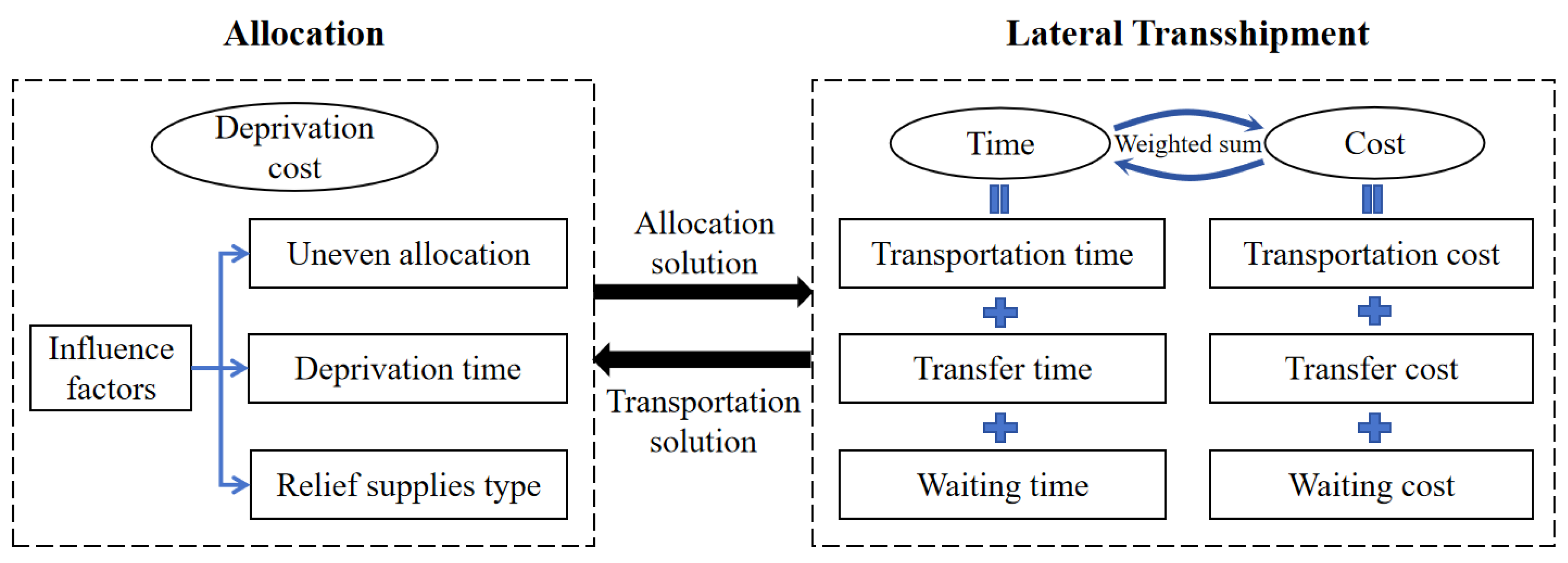
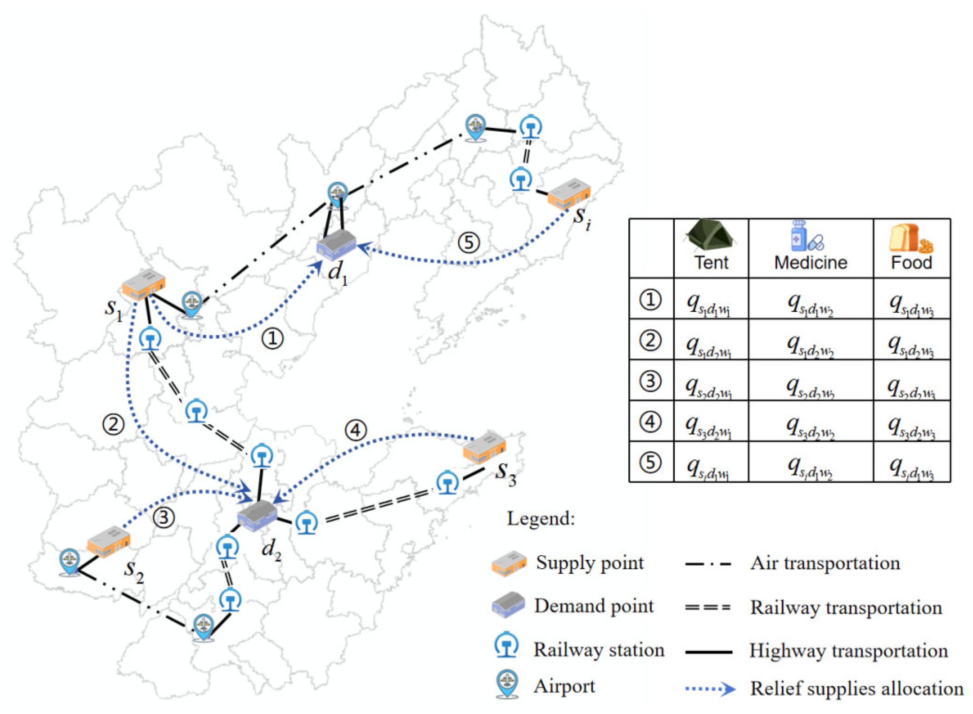
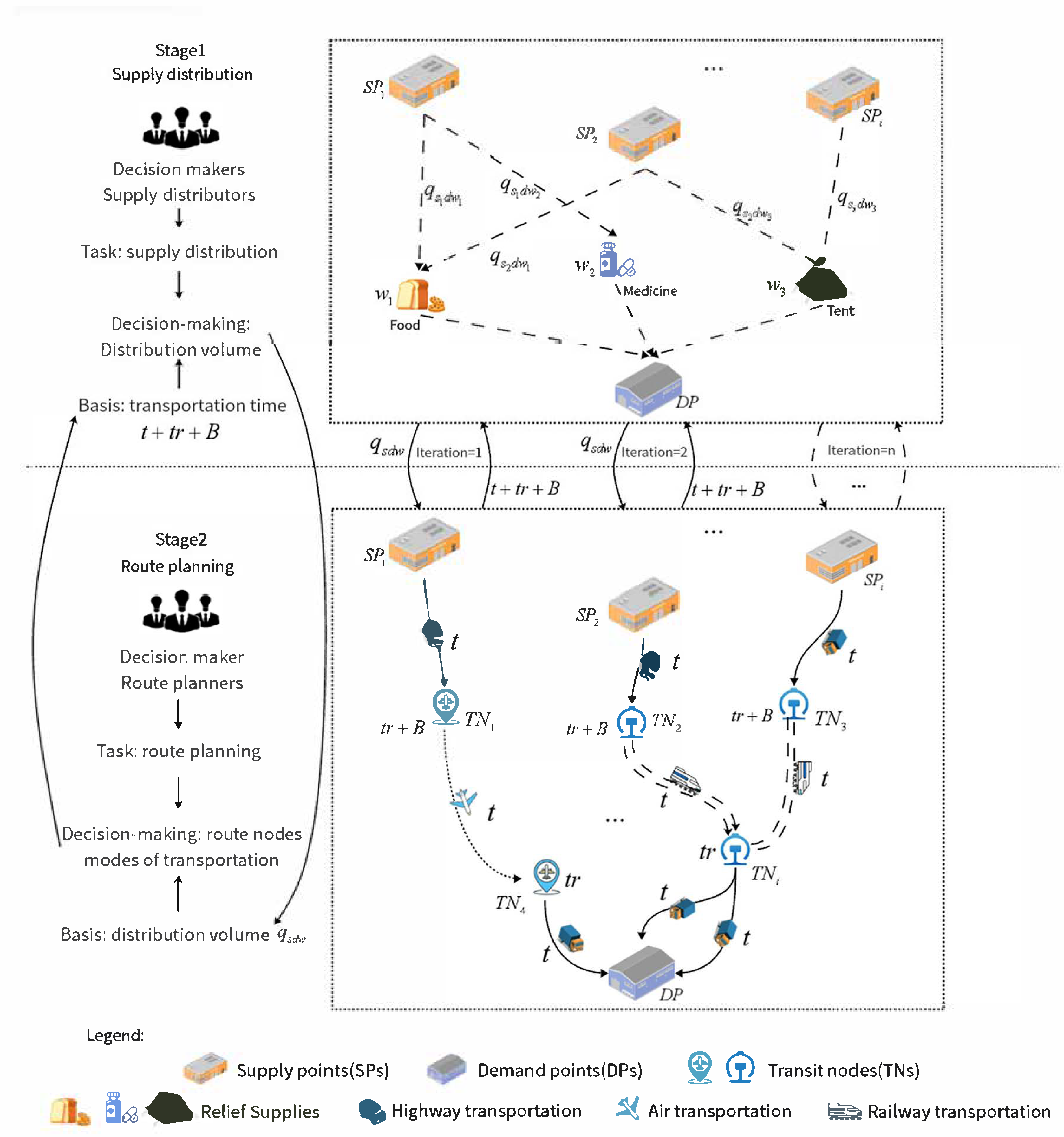
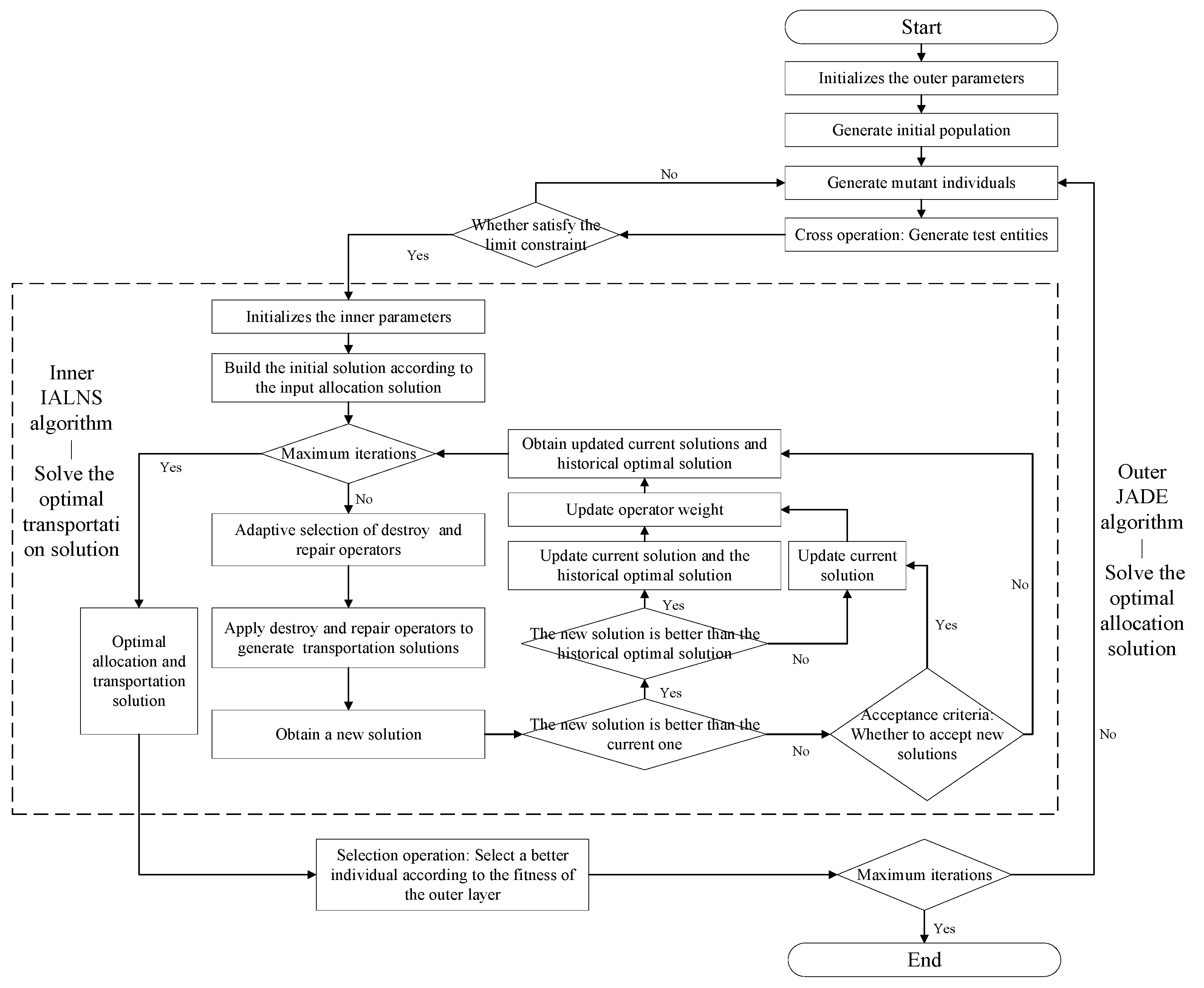
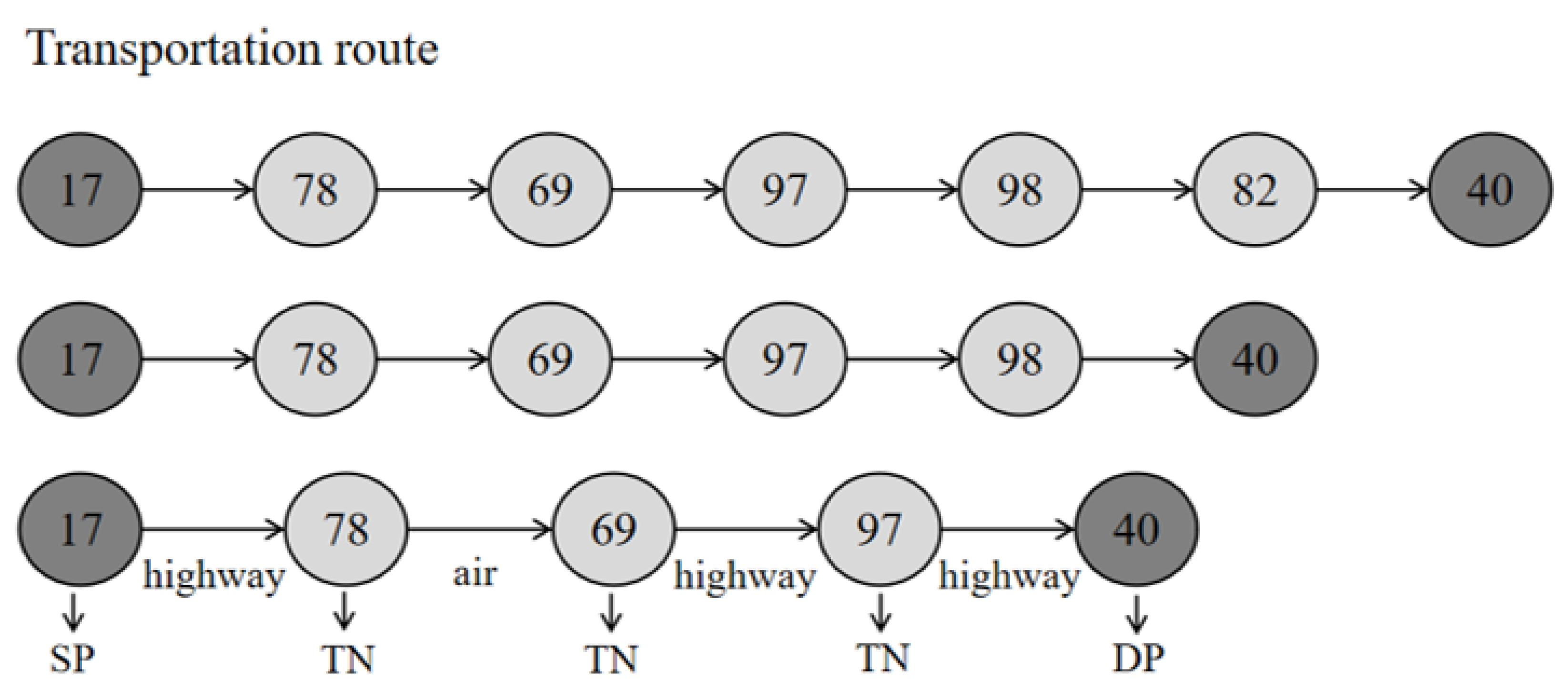
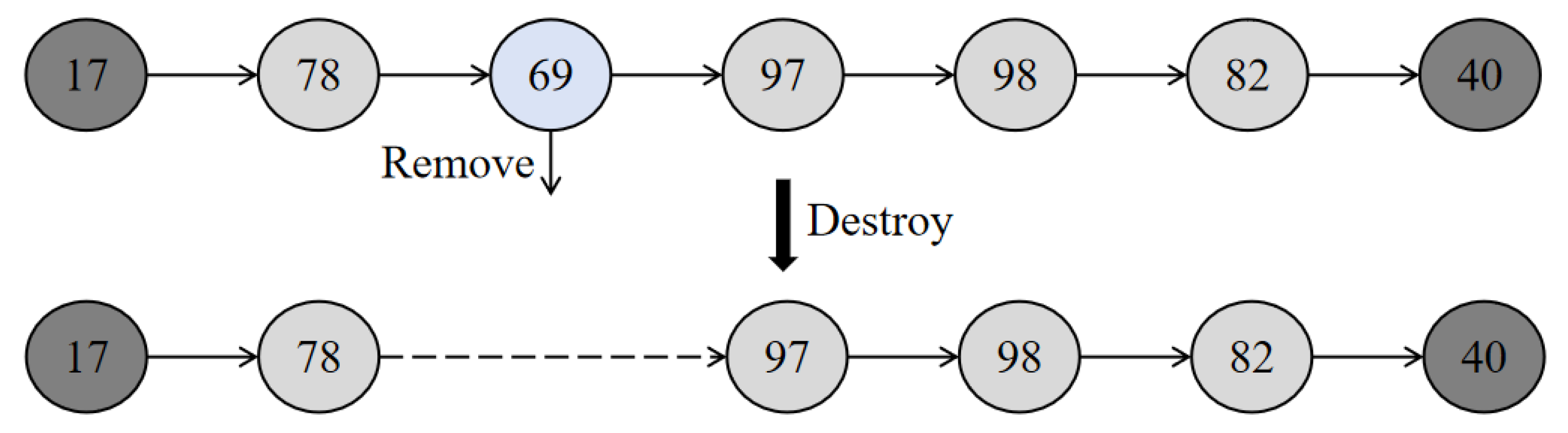
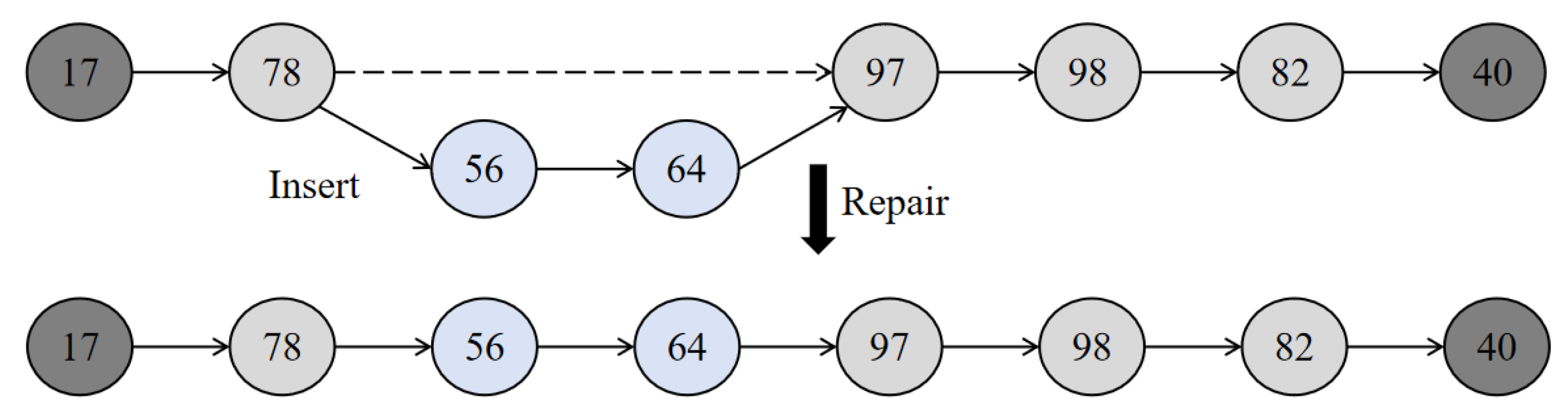
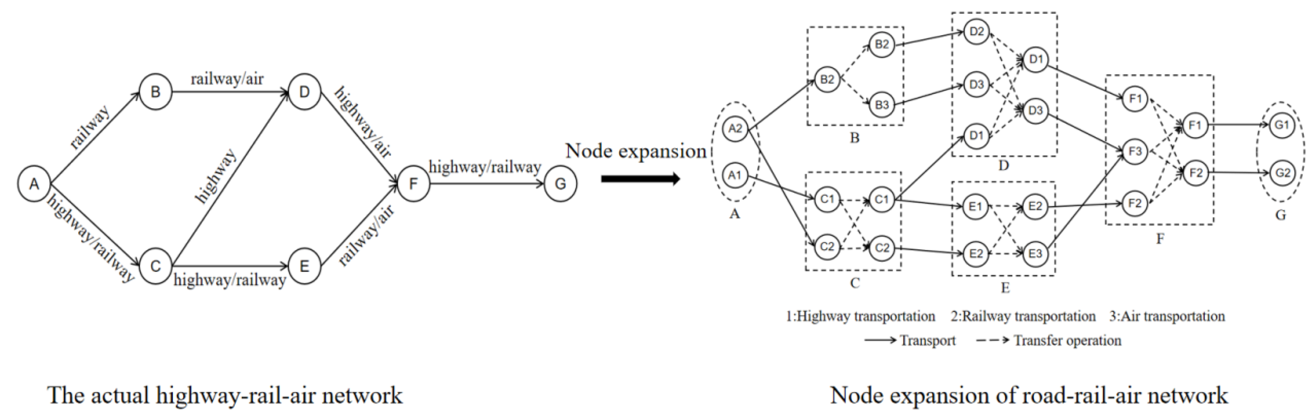
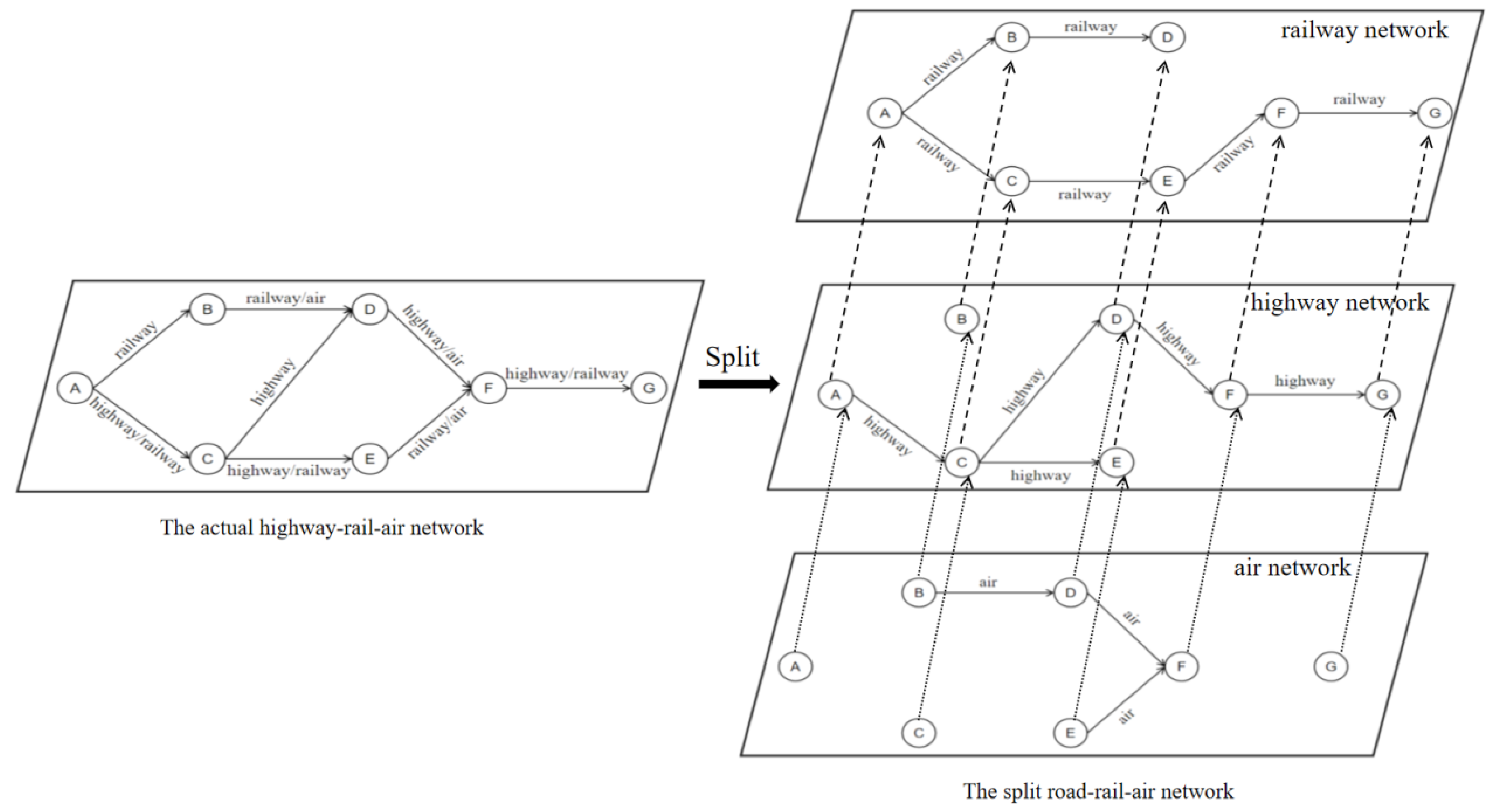
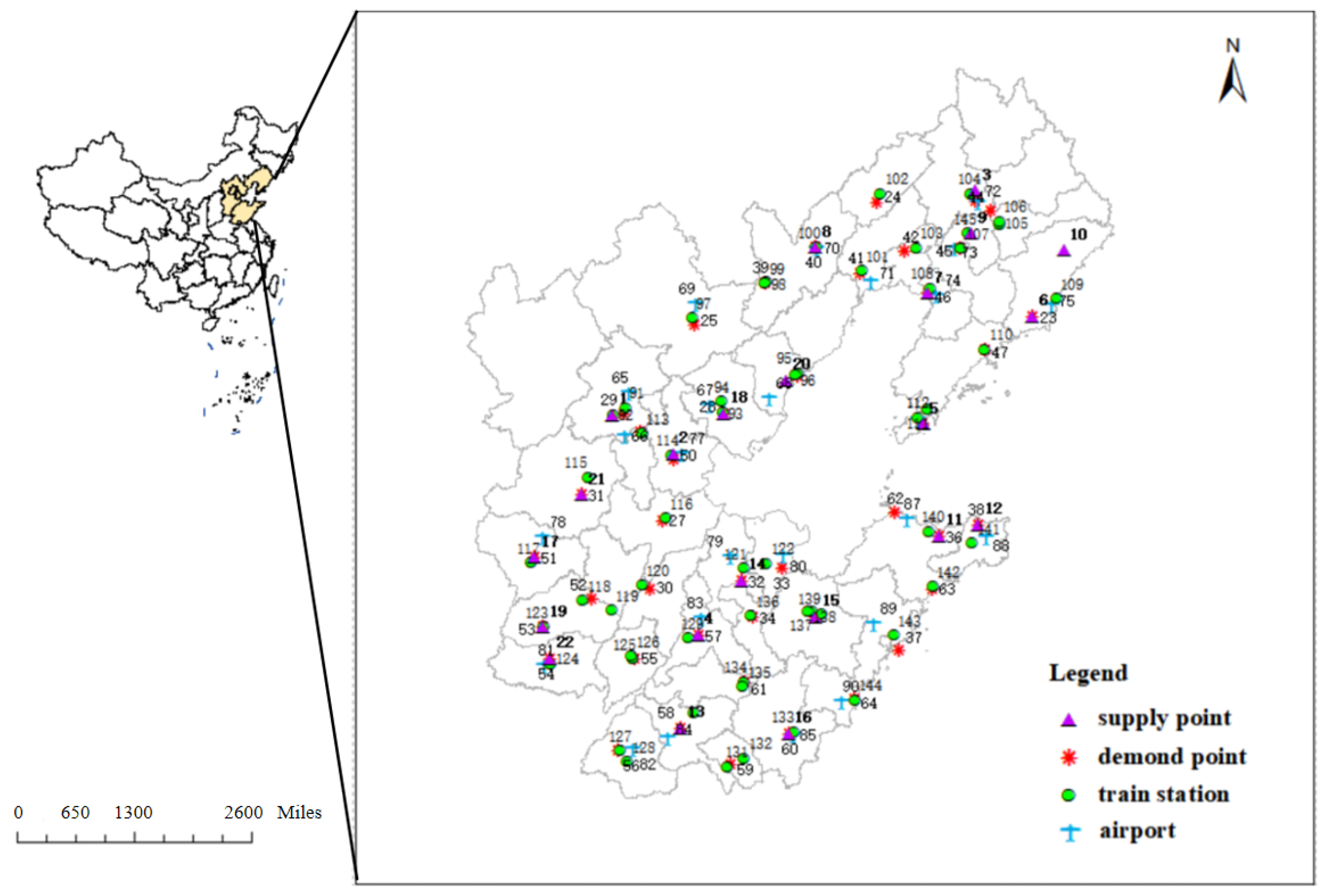
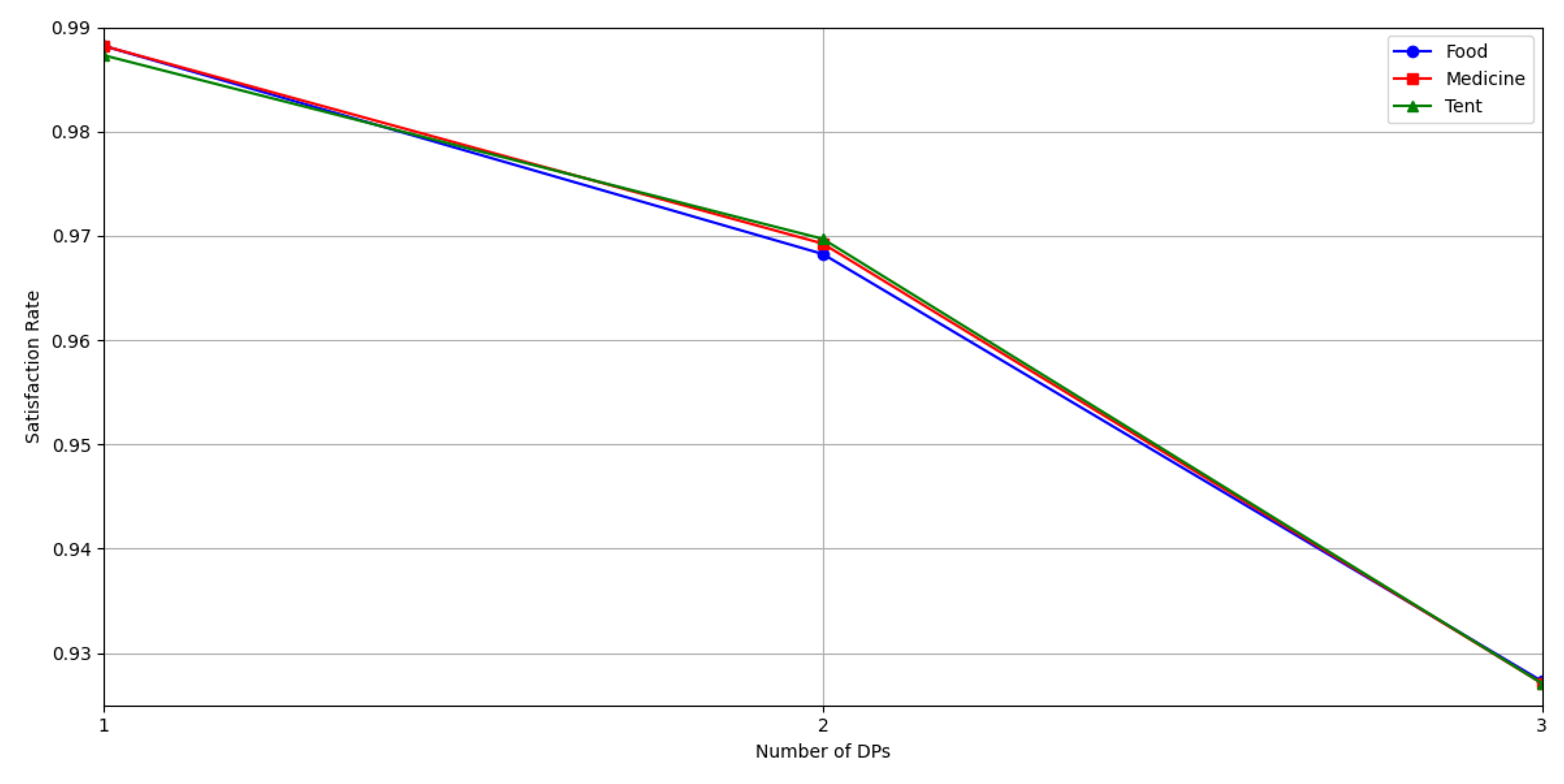
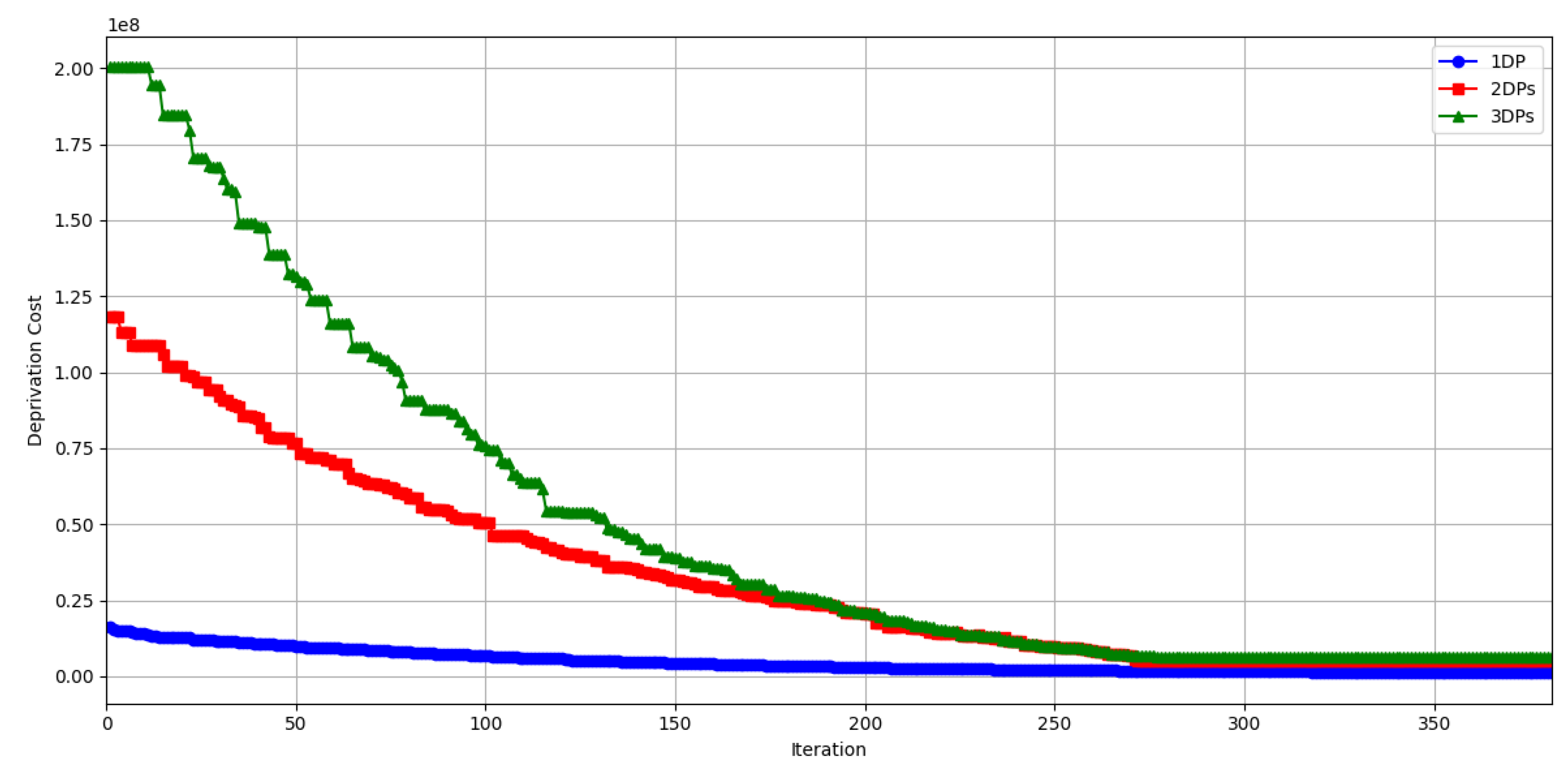
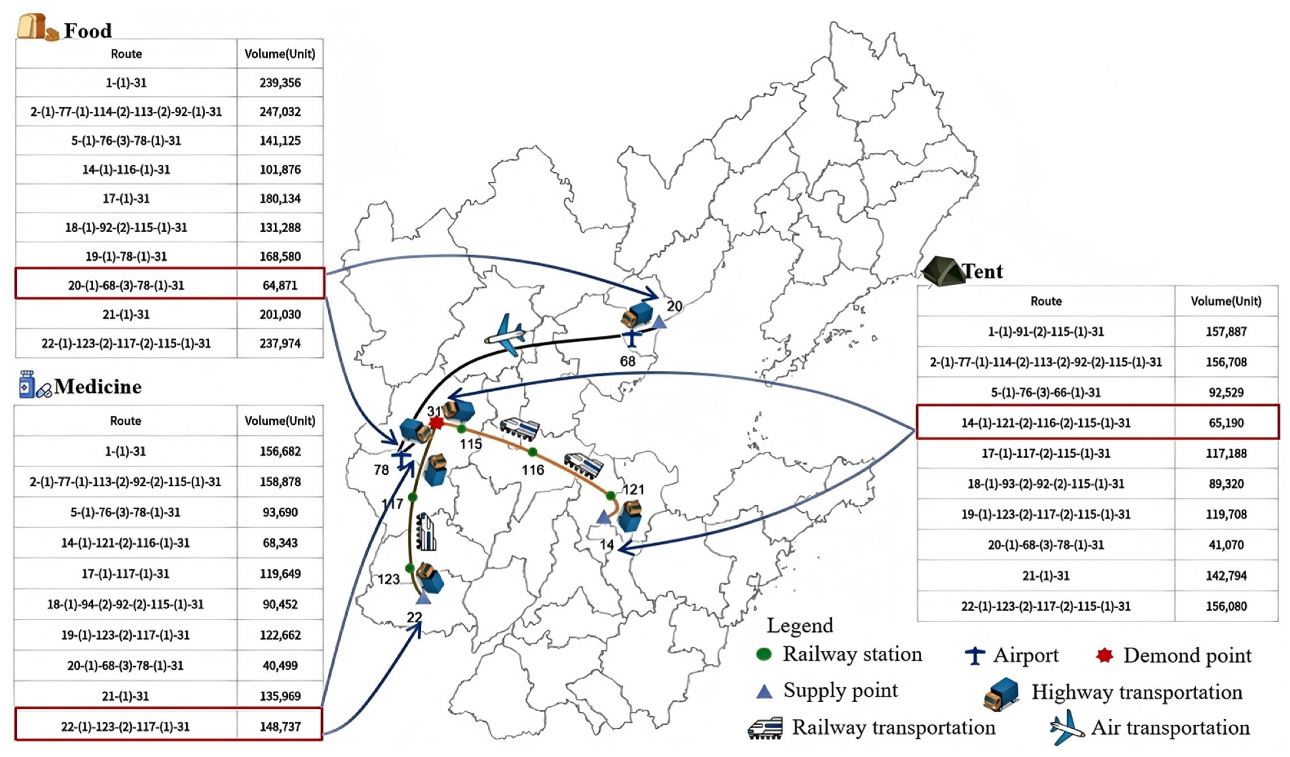
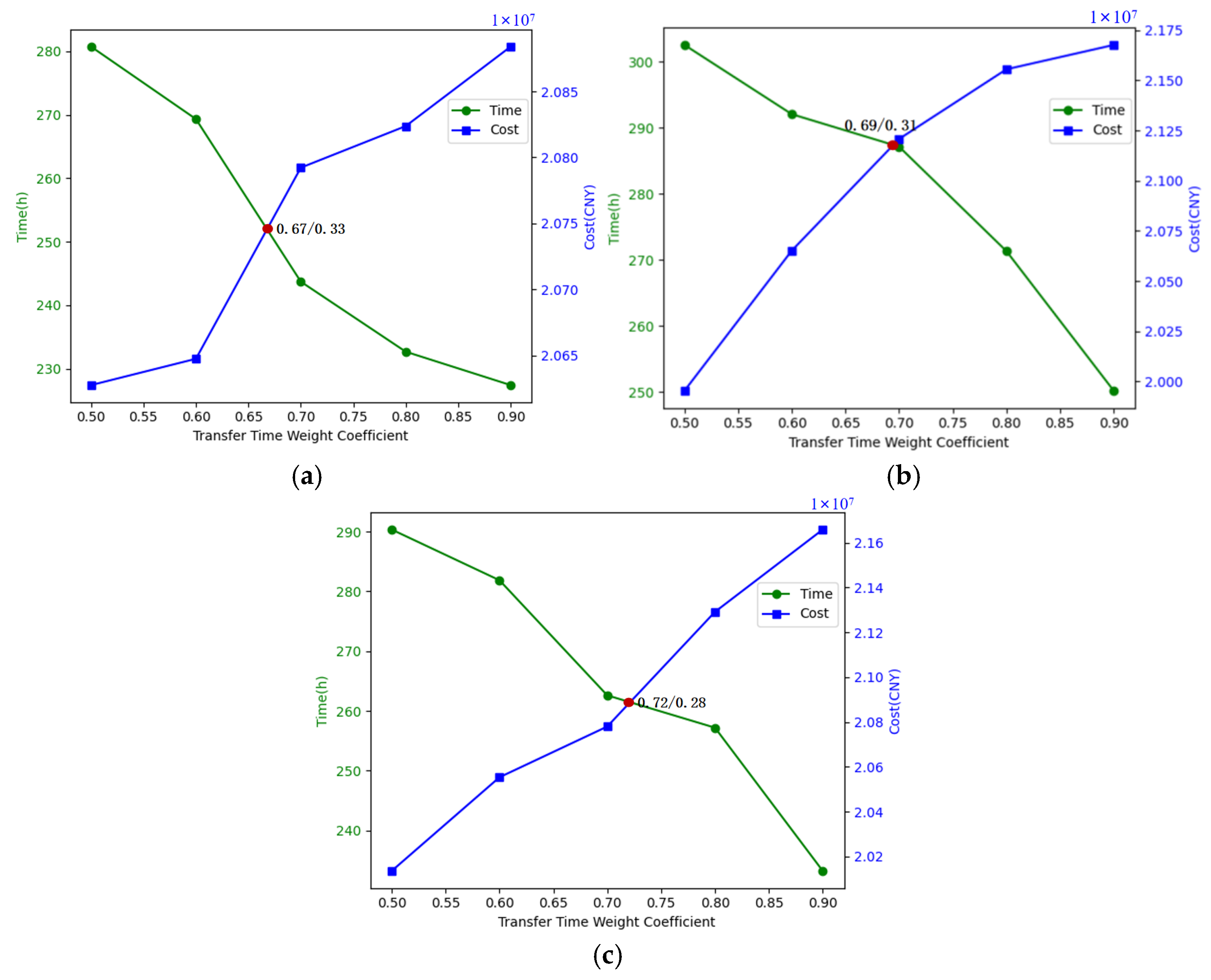
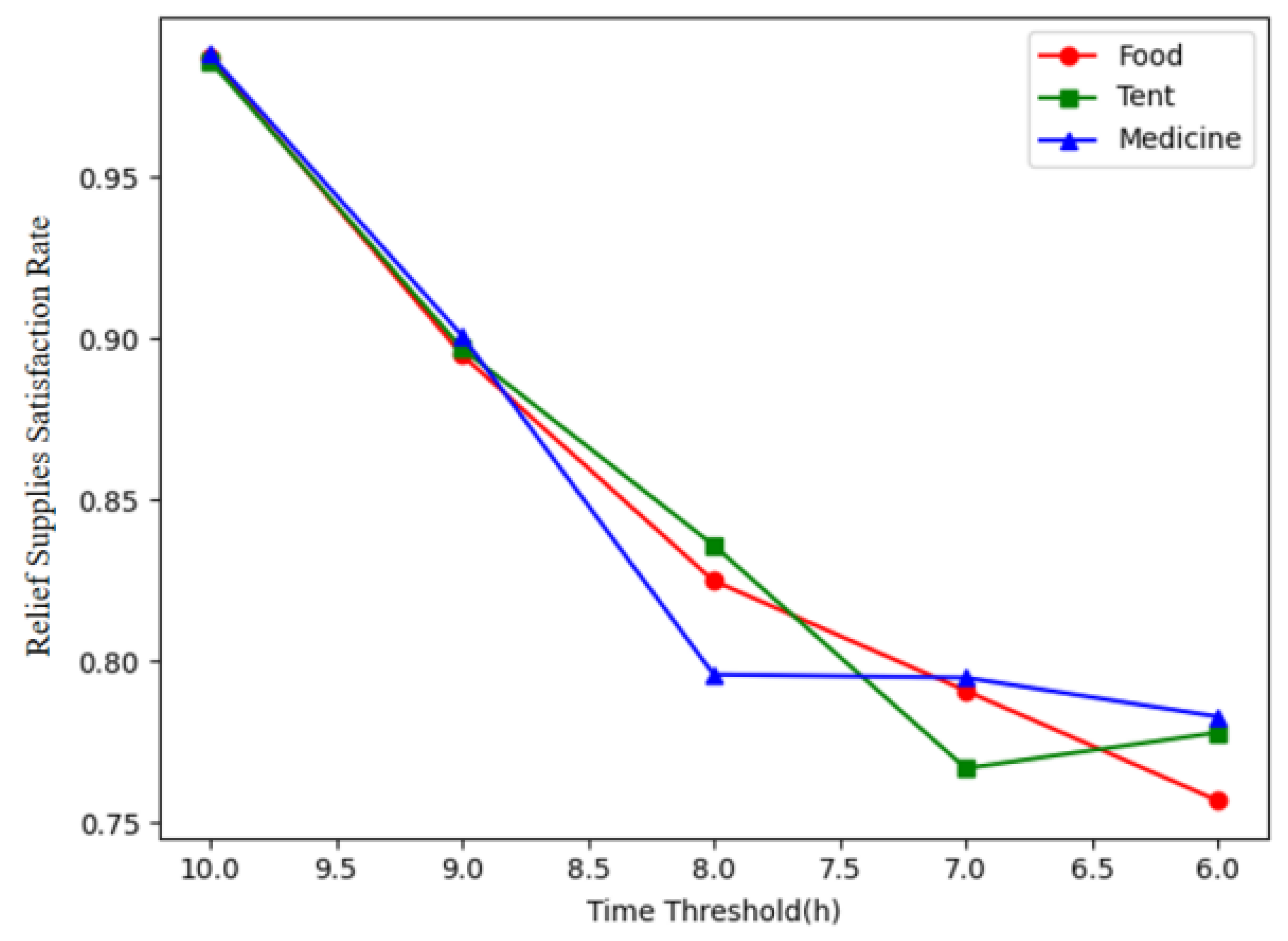
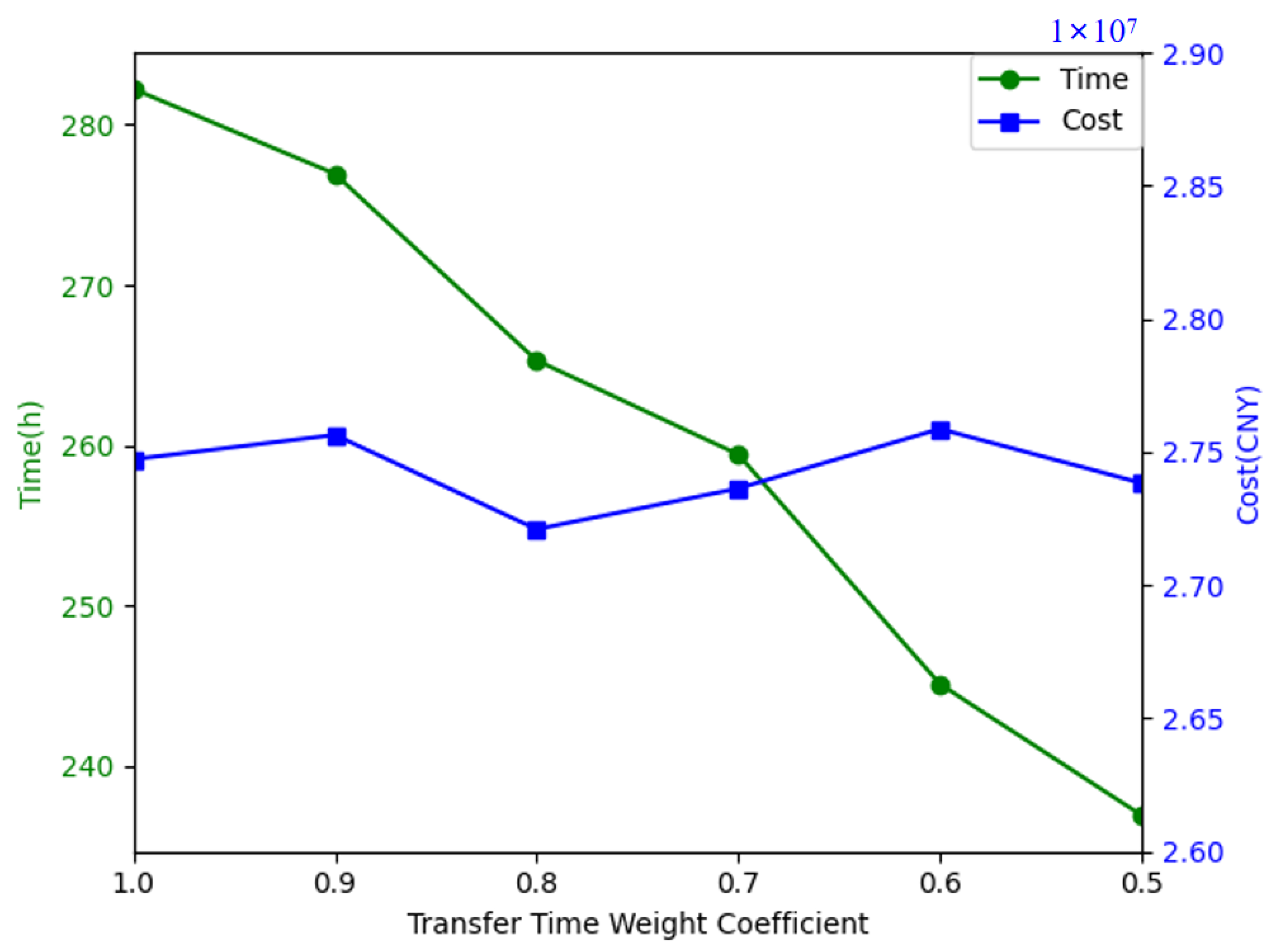
Disclaimer/Publisher’s Note: The statements, opinions and data contained in all publications are solely those of the individual author(s) and contributor(s) and not of MDPI and/or the editor(s). MDPI and/or the editor(s) disclaim responsibility for any injury to people or property resulting from any ideas, methods, instructions or products referred to in the content. |
© 2025 by the authors. Licensee MDPI, Basel, Switzerland. This article is an open access article distributed under the terms and conditions of the Creative Commons Attribution (CC BY) license (https://creativecommons.org/licenses/by/4.0/).