Recent Advances in Optimization Methods for Machine Learning: A Systematic Review

Abstract

This systematic review explores modern optimization methods for machine learning, distinguishing between gradient-based techniques using derivative information and population-based approaches employing stochastic search. Key innovations focus on enhanced regularization, adaptive control mechanisms, and biologically inspired strategies to address challenges like scaling to large models, navigating complex non-convex landscapes, and adapting to dynamic constraints. These methods underpin core ML tasks including model training, hyperparameter tuning, and feature selection. While significant progress is evident, limitations in scalability and theoretical guarantees persist, directing future work toward more robust and adaptive frameworks to advance AI applications in areas like autonomous systems and scientific discovery.

1. Introduction

Machine learning has witnessed transformative progress driven by deep neural networks [1] and generative architectures such as transformers [2] and diffusion models [3]. These innovations enable unprecedented performance in tasks that span perception, language understanding, and content synthesis, marking a shift toward scalable and adaptive systems.

However, the practical realization of these advances hinges on solving complex optimization problems. Training objectives typically combine empirical risk minimization (e.g., cross-entropy loss for classification) and regularization (e.g., $L_1$/$L_2$ penalties) to balance accuracy and generalization [4,5]. Although unconstrained optimization suffices for tasks such as linear regression [6], modern applications demand constrained formulations, from fairness-aware learning [7] to non-negative matrix factorization [8]. Recent studies highlight the challenges of scaling optimization to trillion-parameter models, where adaptive momentum clipping, memory-efficient strategies, and second-order methods such as natural gradient [9] and the memory-efficient framework proposed by Liu et al. [10] become critical to prevent divergence. A critical challenge lies in the duality between regularization and explicit constraints: $L_1$ regularization, for example, induces sparsity equivalent to a constraint on the $L_1$ norm [6]. Furthermore, non-convex landscapes in deep networks, dynamic constraints in reinforcement learning, and scalability limits in distributed training necessitate novel algorithms. Emerging paradigms demonstrate how domain-specific knowledge can be integrated into learning frameworks to tackle nontraditional optimization landscapes. Addressing these optimization bottlenecks is essential to advance both theoretical rigor and real-world deployment, particularly as models grow in complexity and societal requirements for robustness and interpretability intensify. Distributed training frameworks require specialized communication optimizations [11] to maintain efficiency. A fundamental analysis of deep network training difficulties [12] reveals gradient-related pathologies that constrain trillion-parameter optimization.

Optimization methods can be systematically categorized into two fundamental paradigms based on their computational frameworks: gradient-based methods and population-based approaches. And they are placed formally in Figure 1 below. Fundamental analysis of deep network training difficulties reveals gradient-related pathologies that constrain trillion-parameter optimization.

These complementary approaches address core challenges including high-dimensional parameter spaces, non-convex landscapes, and dynamic constraints. Gradient-based methods excel in data-rich scenarios requiring rapid convergence, while population-based approaches dominate problems with unavailable derivative information. Fundamental complexity trade-offs [13] govern algorithm selection for these scenarios.

It is evident that optimization methods mainly affect machine learning in three ways: model training; feature selection and dimensionality reduction; and hyperparameter optimization. In model training, these algorithms enable effective parameter adjustment, accelerate convergence, and enhance generalization capabilities by helping models learn complex patterns from data. Their application extends to feature engineering, where optimization techniques identify informative feature subsets through selection and dimensionality reduction, improving computational efficiency while maintaining model interpretability in high-dimensional domains like image processing and bioinformatics. Furthermore, optimization methods prove indispensable for hyperparameter tuning, systematically exploring parameter spaces to discover optimal configurations that maximize model performance while conserving computational resources. Collectively, these optimization-driven approaches form the backbone of modern deep learning systems, balancing computational feasibility with enhanced predictive accuracy across diverse applications.

During the application of optimization methods, several challenges arise, including high-dimensional problems, multimodal optimization problems and optimization in dynamic environments. High-dimensional optimization problems involve vast search spaces that exponentially grow with dimensionality, leading to high computational costs, slow convergence, degraded generalization stability [14], and an increased risk of getting trapped in the local optima. Multimodal optimization problems feature multiple local optima, which can mislead optimization algorithms away from the global optimum, making it necessary to balance diversity and computational complexity to find the best solutions. Optimization in dynamic environments requires algorithms to adapt quickly to changes in objectives or constraints, necessitating real-time adjustments and the effective use of historical data to maintain performance. These challenges demand more efficient, robust, and adaptive optimization algorithms, driving ongoing research into enhancing existing methods and developing innovative strategies to overcome these hurdles.

These optimization methods demonstrate broad applicability across machine learning domains: gradient-based techniques like AdamW [15] (decoupled weight decay), Adamax [16] ($L_{\infty }$-norm stabilization), AMSGrad [17] (historical maximum tracking), Adai [18] (adaptive inertia), NovoGrad [19] (layer-wise normalization), AdamP [20] (projected gradient normalization), NAdam [21] (Nesterov acceleration), QHAdam [22] (quasi-hyperbolic discounting), RAdam [23] (rectified variance control), LAMB [24] (layer-wise adaptive batch scaling), Look-ahead [25] (dual-weight exploration), and LION [26] (sign-based momentum) excel in deep learning model training and hyperparameter optimization, while population-based approaches including CMA-ES [27] (covariance matrix adaptation), LM-MA [28] (limited-memory evolution), HHO [29] (energy-driven prey pursuit), AVOA [30] (starvation-rate dynamics), AOA [31] (arithmetic operator balancing), NOA [32] (foraging–caching strategies), EDO [33] (exponential distribution properties), and IARO [34] (center-driven refinement with Gaussian wandering) prove effective for feature selection, dimensionality reduction, and complex hyperparameter tuning tasks. Their versatility addresses diverse optimization challenges spanning high-dimensional parameter spaces, non-convex landscapes, and dynamic environments across machine learning applications.

Implementations rely on frameworks including TensorFlow 2.10 [35] and PyTorch 2.1.0 [36], which provide essential automatic differentiation and distributed training support.

The rise of big data and cloud computing presents transformative opportunities for optimization methods, enabling scalable solutions to handle massive datasets and complex models through distributed computing frameworks. In addition, the integration of deep learning with reinforcement learning opens new avenues for adaptive optimization strategies, where models can dynamically refine their learning processes in response to evolving environments. These advances promise more efficient resource utilization and improved adaptability in real-world applications.

Future research should refine optimization techniques for non-convex challenges (convergence stability, efficiency) while exploring novel paradigms (bio-inspired, hybrid) for complex problems. Critical open problems include enhancing limited-data optimization with reduced variance/overfitting; solving non-convex challenges in deep networks to escape local optima; mitigating biases in stochastic optimization for long sequences; and integrating higher-order gradients into variational inference for large-scale efficiency. Application expansion in autonomous systems, climate modeling, and healthcare will further test method robustness.

Following this introduction, the paper proceeds with a systematic analysis organized into four core sections. Section 2 establishes a unified taxonomy of modern optimization methods, categorizing them into gradient-based and population-based paradigms. This section examines their theoretical foundations, core innovations, and comparative trade-offs through the integrated framework illustrated in Figure 1 and

Table 1. Comparative analysis of optimization paradigms.

Characteristics	Gradient-Based Methods	Population-Based Methods
Core Mechanism	Derivative-driven local search	Stochastic population evolution
Key Algorithms	AdamW [15], LION [26], RAdam [23], LAMB [24], AMSGrad [17], NovoGrad [19], Adai [18], NAdam [21], QHAdam [22], AdamP [20], Adamax [16], Look-ahead [25]	AOA [31], NOA [32], IARO [34], EDO [33], CMA-ES [27], LM-MA [28], HHO [29], AVOA [30]
Computational Efficiency	High efficiency	Moderate efficiency
Global Search Ability	Local convergence guarantees	Global exploration capability
Memory Requirements	Moderate state storage	High population maintenance
Optimal Use Cases	Deep network parameter optimization	Hyperparameter tuning, non-convex problems

. Section 3 then explores practical applications across key machine learning domains including deep learning, reinforcement learning, and hyperparameter optimization. Section 4 discusses critical challenges such as high-dimensional scalability and dynamic constraints while synthesizing emerging innovations like bio-mathematical hybrids. The review concludes in Section 5 by summarizing the key insights and outlining future research directions.

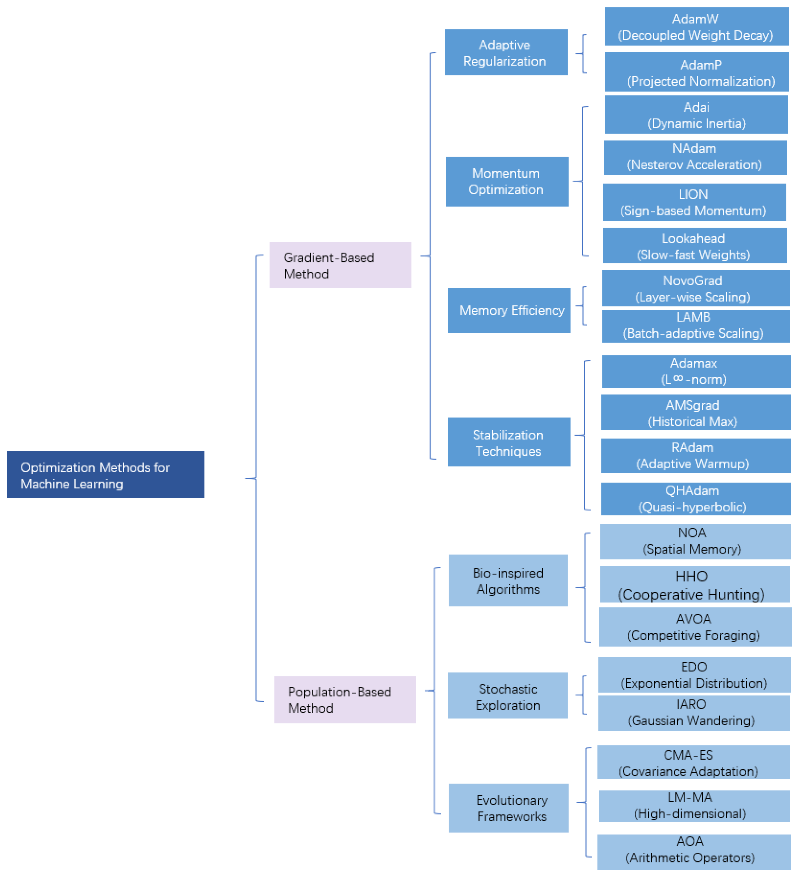
2. Optimization Methods for Machine Learning

This section systematically reviews state-of-the-art optimization algorithms, categorized into two fundamental paradigms: gradient-based methods and population-based methods. They are well arranged in Table 1. These complementary approaches address core challenges in machine learning optimization including high-dimensional parameter spaces, non-convex landscapes, and dynamic environments.

Gradient-based methods leverage derivative information for precise optimization. Section 2.1 details 12 advanced variants focusing on innovations in regularization mechanisms, memory efficiency, and convergence stabilization.

Population-based algorithms employ stochastic search strategies inspired by natural systems [37]. Section 2.2 examines eight state-of-the-art techniques featuring biological inspiration, mathematical foundations, and hybrid strategies.

These dual paradigms provide comprehensive coverage of modern optimization needs, with gradient methods excelling in data-rich scenarios requiring rapid convergence, while population approaches dominate complex problems where derivative information is unavailable or insufficient.

2.1. Gradient-Based Methods

Fundamental stochastic optimization frameworks, including SGD and its variants [38,39,40], established convergence guarantees of $\mathcal{O}(1/\sqrt{T})$ for convex objectives [41]. Momentum acceleration [42,43] and adaptive preconditioning (e.g., AdaGrad [44] and RMSprop [45]) later addressed ill-conditioned landscapes, culminating in Adam’s unified framework [16].

2.1.1. AdamW Algorithm

Adaptive gradient methods like Adam often underperform SGD with momentum [46] due to the inequivalence between $L_2$ regularization and weight decay. In SGD [40], weight decay applies directly to parameters:

$${\theta }_{t+1}=(1-\lambda ){\theta }_t-\alpha \nabla f_t\left({\theta }_t\right).$$

(1)

However, adaptive optimizers scale regularization gradients proportionally to historical gradient magnitudes, weakening regularization for large-gradient parameters. AdamW addresses this by decoupling weight decay from gradient scaling [15]:

$${\widehat{\theta }}_{t+1}=(1-\lambda ){\theta }_t-\alpha M_t\nabla f_t\left({\theta }_t\right).$$

(2)

This modification ensures consistent regularization independent of adaptive preconditioner $M_t$. The equivalent $L_2$ regularization becomes

$$f_t^{reg}\left(\theta \right)=f_t\left(\theta \right)+{\displaystyle \frac{{\lambda }^{\prime }}{2\alpha }}{∥\theta \odot \sqrt{s}∥}_2^2,$$

(3)

amplifying regularization for parameters with large preconditioner values $s_i$.

Empirical validation in Figure 2 shows that AdamW achieves 15% relative test error reduction on CIFAR-10 and ImageNet32x32 [47], closing the generalization gap with SGD. These improvements persist across training budgets (100–1800 epochs) and learning rate schedules, with cosine annealing yielding optimal results. Long-term training confirms AdamW’s superior generalization even at matched training loss values.

AdamW bridges the gap between adaptive methods and SGD by resolving ineffective regularization. Its decoupled weight decay mechanism preserves adaptive learning benefits while enhancing generalization across diverse deep learning tasks.

2.1.2. AdamP Algorithm

AdamP’s core innovation is “Projected Gradient Normalization” [20]. This mechanism specifically addresses suboptimal optimization in layers whose functionality depends primarily on parameter direction rather than magnitude (e.g., scale parameters Y, g in normalization layers like BatchNorm or LayerNorm).

The central mathematical operation is a vector projection. Before calculating the adaptive learning rate terms, AdamP projects the raw gradient vector onto the direction orthogonal to the current parameter vector. The core formula is

$$g_{perp}=g_t-{\displaystyle \frac{g_t\ast {\theta }_t}{\parallel {\theta }_t{\parallel }^2}}*{\theta }_t,$$

(4)

where $g_t$ is the raw gradient, and ${\theta }_t$ denotes the parameter vector. $g_{perp}$ is the gradient component perpendicular to ${\theta }_t$. ${\displaystyle \frac{(g_t\ast {\theta }_t)}{\parallel {\theta }_t{\parallel }^2}}\ast {\theta }_t$ represents the projection of the gradient onto ${\theta }_t$ (the radial component, changing magnitude).

AdamP then uses $g_{perp}$ to update Adam’s first moment $m_t$ and second moment $v_t$ [16] estimates. The subsequent parameter update retains the AdamW [15] form

$${\theta }_{t+1}={\theta }_t-\eta \ast {\displaystyle \frac{{\widehat{m}}_t}{\sqrt{{\widehat{v}}_t+ϵ}}}-\eta \ast \lambda \ast {\theta }_t.$$

(5)

With these mechanisms, the adaptive update term ${\displaystyle \frac{{\widehat{m}}_t}{\sqrt{{\widehat{v}}_t+ϵ}}}$, which is now driven by $g_{perp}$, exclusively optimizes the parameter’s direction. And the weight decay term $-\eta \ast \lambda \ast {\theta }_t$ independently controls the parameter’s magnitude (norm).

This elegant separation aligns perfectly with the properties of normalization layer scale parameters. By preventing the adaptive mechanism from inefficiently fighting weight decay over magnitude changes, and focusing it purely on directional updates, AdamP achieves more stable optimization and often superior final model performance compared to AdamW.

2.1.3. Adai Algorithm

The Adai (Adaptive Inertia) [18] optimizer addresses the late-stage convergence instability observed in adaptive optimizers like Adam [16]. Traditional methods use a fixed momentum decay rate ${\beta }_1$, which can cause oscillatory behavior near optimal solutions during later training phases. Adai’s innovation lies in its dynamically adjusted inertial coefficient ${\beta }_t$, computed in real time, based on the directional alignment between the current gradient $g_t$ and historical momentum $m_{t-1}$:

$${\beta }_t=max(0,1-{\displaystyle \frac{g_t^{\mathsf{T}}{m}_{t-1}}{\parallel g_t{\parallel }^2}}).$$

(6)

This mechanism preserves high inertia when gradients and momentum align (accelerating convergence) but reduces inertia during directional conflicts (preventing oscillations), achieving an optimal balance between speed and stability. The Lottery Ticket Hypothesis [48] provides theoretical grounding for sparse trainable subnetworks relevant to inertia control [18].

Adai achieves what Adam cannot: provable convergence in both convex and non-convex landscapes. Its adaptive inertia intrinsically satisfies the directional consistency condition—a mathematical requirement for convergence where fixed-inertia optimizers fail. For convex objectives, Adai guarantees arrival at global minima. In complex non-convex terrains, it converges to stationary points where gradients vanish, overcoming Adam’s oscillation pitfalls.

Benchmarks reveal Adai’s late-training superiority. In ResNet/CIFAR-10 and LSTM/Penn Treebank tasks, it outperforms Adam by 0.5%–2% test accuracy during final training stages while maintaining early-stage parity. The 1%–3% computational overhead (from gradient-momentum dot products) is offset by a reduced need for learning rate scheduling [18]. Adai particularly excels in transformer architectures and sharp-minima problems where Adam exhibits validation loss oscillations.

Optimal results emerge with learning rates 2-3× larger than Adam’s typical settings. The algorithm shines in stable convergence scenarios but requires gradient clipping in high-sparsity applications like recommendation systems. Avoid deployment on ultra-low-power devices where the dot-product overhead becomes prohibitive.

2.1.4. NAdam Algorithm

The Nesterov-accelerated Adaptive Moment Estimation (NAdam) [21,49], fundamentally fuses Adam [16] with the Nesterov momentum. It combines Adam’s adaptive learning rates with the “look-ahead” property of the Nesterov momentum (NAG) to achieve faster and more stable convergence.

The core innovation of NAdam simulates NAG’s “look-ahead” update. In NAG, a “look-ahead” step is first taken to a temporary point:

$${\theta }_{temp}={\theta }_{t-1}-{\beta }_1\ast {\displaystyle \frac{m_{t-1}}{1-{\beta }_1^{t-1}}}.$$

(7)

Then the gradient is computed at this point rather than the temporary point to avoid the redundancy calculation update. NAdam achieves look-ahead via mathematical approximation. The look-ahead momentum estimate ${\widehat{m}}_t$ is calculated as

$${\widehat{m}}_t^{nesterov}={\beta }_1·{\displaystyle \frac{m_t}{1-{\beta }_1^t}}+(1-{\beta }_1)·{\displaystyle \frac{g_t}{1-{\beta }_1^t}}.$$

(8)

This formula approximates the momentum state at the look-ahead point ${\theta }_{temp}$ by weighting the current bias-corrected momentum ${\widehat{m}}_t^{nesterov}$ with the decay coefficient of the next step ${\beta }_1^{t+1}$, then blending in the current gradient $g_t$. Then this look-ahead momentum estimate replaces the momentum estimate of Adam. The final parameter update becomes

$${\theta }_t={\theta }_{t-1}-\alpha ·{\displaystyle \frac{{\widehat{m}}_t^{nesterov}}{\sqrt{{\widehat{v}}_t}+ϵ}},$$

(9)

where the second-moment estimate $v_t$ and its bias correction ${\widehat{v}}_t$ retain the same as Adam. Its strength lies in the dual inheritance: NAdam retains Adam’s advantages—adaptive learning rates effective for sparse gradients and ill-scaled features—while gaining the NAG look-ahead property. This allows the earlier detection of gradient changes near optima, reducing oscillations and accelerating convergence. The computational cost matches Adam. Default Adam hyperparameters ($\alpha =0.001$, ${\beta }_1=0.9$, ${\beta }_2=0.999$, $ϵ=1e-8$) typically work well, making NAdam a superior drop-in replacement when standard Adam exhibits oscillation or slow convergence.

2.1.5. LION Optimization Algorithm

Adaptive optimizers like Adam [16] and Adafactor [22] face limitations in generalization and memory overhead due to second-moment estimation. Alternative approaches like AdaBound [50] dynamically constrain learning rates to stabilize convergence. Lion addresses these issues by reducing memory usage by 50% through tracking only momentum $m_t$ instead of two moments.

Lion’s core innovation is the sign-based parameter update:

$$updat{e}_t=sign({\beta }_1{m}_{t-1}+(1-{\beta }_1)g_t),$$

(10)

where ${\beta }_1=0.9$. This uniform update magnitude across dimensions eliminates second-moment tracking while introducing stochastic regularization. The momentum term balances short/long-term gradient information:

$$m_t={\beta }_2{m}_{t-1}+(1-{\beta }_2)g_t,$$

(11)

with ${\beta }_2=0.99$ ensuring stability in large-batch training.

Lion was discovered through regularized evolution in symbolic program space. Abstract execution techniques pruned redundant operations from Adam-like initializations, yielding the concise Lion algorithm.

Lion demonstrates significant performance gains across diverse domains. It boosts Vision Transformers’ ImageNet accuracy by up to 2% while reducing pretraining costs 5×. In vision-language tasks, it achieves 88.3% zero-shot accuracy (+2% SOTA) and 91.1% fine-tuning accuracy. For diffusion models, Lion reduces training iterations 2.3× while improving the sample quality. The 50% memory reduction proves critical for large models like ViT-H/14 and T5-11B.

Lion represents a paradigm shift in optimizer design, combining evolutionary search with mathematical simplicity. Its sign-based updates and dual EMA momentum enable memory efficiency, computational speed, and robust generalization across vision, language, and generative tasks.

2.1.6. Look-Ahead Algorithm

The Look-ahead optimizer is a generalized wrapper framework for optimization algorithms. It addresses oscillation and generalization limitations in traditional deep learning optimizers through a decoupled exploration-averaging mechanism. This approach maintains two sets of weight parameters: fast weights $\varphi$ conduct rapid exploration in parameter space, while slow weights $\theta$ perform careful averaging, creating a unique dual-weight optimization system [25].

Given a base optimizer like Adam or SGD, Look-ahead operates with key parameters: synchronization period k (typical values 5-20), slow weights learning rate $\alpha$ (typically 0.5), and loss function $\mathcal{L}$. The algorithm alternates between two distinct phases: an inner-loop exploration stage and an outer-loop averaging stage.

During the inner-loop exploration phase, fast weights $\varphi$ undergo k steps of base optimizer updates:

$${\varphi }_{t+1}=\mathrm{BaseOptimizer}({\varphi }_t,\nabla \mathcal{L}\left({\varphi }_t\right)).$$

(12)

Throughout this phase, slow weights $\theta$ remain stationary, allowing $\varphi$ to thoroughly explore the loss landscape. In the outer-loop averaging phase, slow weights $\theta$ update through linear interpolation toward the current fast weights position:

$${\theta }_{n}ew=(1-\alpha )\theta +\alpha {\varphi }_k.$$

(13)

The fast weights then reset to the new slow weights position: ${\varphi }_0={\theta }_{\mathrm{new}}$. This periodic reset mechanism smooths the optimization trajectory.

Look-ahead significantly enhances training stability by reducing loss oscillation variance and simultaneously improves hyperparameter robustness, particularly reducing sensitivity to the base optimizer’s learning rate. It fundamentally differs from the Exponential Moving Average (EMA): While Look-ahead performs discrete linear interpolation ${\theta }_{\mathrm{new}}=(1-\alpha )\theta +\alpha \varphi$, EMA employs continuous exponential smoothing ${\theta }_{\mathrm{ema}}=\beta {\theta }_{\mathrm{ema}}+(1-\beta )\theta$. Crucially, Look-ahead’s slow weights $\theta$ directly participate in gradient computation, whereas EMA weights serve only for the final inference.

The synchronization period k controls the exploration depth: for smaller datasets, $k\in [3,5]$ enhances stability, while complex tasks benefit from $k\in [10,20]$ to strengthen exploration. The slow weights learning rate $\alpha$ balances exploration and stability: recommended at $\alpha =0.5$ with tuning range $\alpha \in [0.3,0.8]$. The base optimizer’s learning rate can be moderately increased to 1.0–1.5 times its original value.

Through its innovative dual-weight update system—fast weights $\varphi$ performing k exploration steps and slow weights $\theta$ executing periodic weighted averages—Look-ahead simultaneously enhances training stability and generalization power. Empirical results demonstrate consistent performance gains of 1–2%, establishing it as an effective universal framework for improving deep learning optimization processes.

2.1.7. NovoGrad Algorithm

NovoGrad [19] is an adaptive optimizer designed for the memory-efficient training of large-scale deep neural networks. Its core innovation lies in performing gradient normalization per parameter tensor (layer) rather than per individual weight element. Its fundamental innovation is layer-wise gradient normalization, replacing the element-wise normalization used in optimizers like Adam.

The layer-wise scalar second moment $v_t^{\left(l\right)}$, for a layer l at step t, is calculated by summing the squared gradients across the entire parameter tensor:

$$v_t^{\left(l\right)}={\beta }_2·v_{t-1}^{\left(l\right)}+(1-{\beta }_2)·{\parallel g_t^{\left(l\right)}\parallel }_2^2,$$

(14)

where $\parallel g_t^{\left(l\right)}{\parallel }_2^2$ represents the sum of squares of all gradient elements in the layer. This scalar $v_t^{\left(l\right)}$ replaces the full-sized second-moment tensor used in Adam. Then this scalar normalizes every gradient element in the layer uniformly:

$${\widehat{g}}_t^{\left(l\right)}={\displaystyle \frac{g_t^{\left(l\right)}}{\sqrt{v_t^{\left(l\right)}+ϵ}}}.$$

(15)

Every element in the gradient tensor $g_t^{\left(l\right)}$ is divided by the same scalar $\sqrt{v_t^{\left(l\right)}+ϵ}$, irrespective of its individual value. This layer-wise normalization contrasts sharply with element-wise operations in other adaptive methods.

The memory reduction stems directly from this design. Storing $v_t^{\left(l\right)}$ as a single scalar per layer reduces the optimizer state memory from $\mathcal{O}\left(n\right)$ (where n is the number of parameters) to $\mathcal{O}\left(L\right)$ (where L is the number of layers). This enables the training of models an order of magnitude larger than would be possible with conventional optimizers under the same memory constraints.

2.1.8. LAMB Algorithm

Large-scale deep learning requires increasing batch sizes to improve hardware utilization and reduce the communication overhead. However, when batch sizes exceed critical thresholds (e.g., >8192 for BERT pretraining), traditional optimizers like Adam/AdamW suffer from convergence degradation. LAMB (Layer-wise Adaptive Moments optimizer for Batch training) solves this via layer-adaptive learning rate scaling, enabling stable training with batch sizes up to 64K+ while maintaining accuracy [24].

LAMB is built upon AdamW [15] and inherits its basic mechanisms. The core innovation of LAMB is the layer-wise trust ratio. The algorithm splits network parameters into distinct layers ${\theta }^{\left(l\right)}$ and computes a dynamic scaling factor for each layer:

$${\varphi }^{\left(l\right)}=min({\displaystyle \frac{\parallel {\theta }_t^{\left(l\right)}{\parallel }_2}{\parallel \Delta {\theta }_t^{\left(l\right)}{\parallel }_2+ϵ}},\gamma ).$$

(16)

This trust ratio ${\varphi }^{\left(l\right)}$ creates a geometric coupling between parameter magnitudes and update vectors. When update directions ($\Delta {\theta }_t^{\left(l\right)}$) are small relative to parameter norms ($|{\theta }_t^{\left(l\right)}{|}_2$), ${\varphi }^{\left(l\right)}\approx 1$ preserves the original update. When updates grow disproportionately large, ${\varphi }^{\left(l\right)}\ll 1$ automatically suppresses the unstable steps. This layer-adaptive scaling eliminates the manual learning rate tuning across network hierarchies.

LAMB delivers three transformative benefits for large-scale training. It shatters batch size barriers, enabling stable convergence at 64K batch sizes where AdamW fails beyond 4K. The algorithm accelerates early convergence, reaching 90% of AdamW’s [15] final accuracy in just 25% of training steps. Crucially, LAMB expands the usable learning rate range to $[{10}^{-4},{10}^{-2}]$, ten times wider than AdamW’s sensitive $[{10}^{-5},{10}^{-3}]$ window. These advantages compound in distributed settings, where LAMB maintains near-linear throughput scaling across thousands of accelerators.

2.1.9. Adamax Algorithm

Adamax [16] emerges as a direct variant of the Adam [16] optimizer within the evolutionary lineage of adaptive learning rate algorithms. Due to a shortcoming in Adam, it often exhibits oscillatory parameter updates when a squaring operation is introduced in the calculation of the $L_2$-norm, which results in amplified disturbance. To address this, Adamax is designed with its featuring innovation to replace the $L_2$-norm with the $L_{\infty }$-norm.

The algorithm transforms the gradient second-moment estimation through a novel approach. While Adam computes $v_t={\beta }_2{v}_{t-1}+(1-{\beta }_2)g_t^2$, Adamax introduces the recursive maximum operation $u_t=max({\beta }_2{u}_{t-1},|g_t\left|\right)$. This $L_{\infty }$-norm estimator $u_t$ tracks the exponentially decaying maximum of absolute gradients. The parameter update simplifies to ${\theta }_t={\theta }_{t-1}-\alpha {\widehat{m}}_t/u_t$, eliminating Adam’s stability constant $\epsilon$ while naturally bounding the update magnitudes. Adamax preserves Adam’s first-moment system $m_t={\beta }_{1}mt-1+(1-{\beta }_1)g_t$ but streamlines bias correction to only ${\widehat{m}}_t=m_t/(1-{\beta }_1^t)$, leveraging the intrinsic properties of the max operation.

Empirical studies reveal Adamax’s three key advantages: accelerated convergence by 10–17% in sparse-gradient domains like natural language processing, reduced hyperparameter sensitivity through the elimination of $\epsilon$ tuning, and approximately 40% fewer training loss spikes. However, in dense-gradient tasks such as image classification, the $max(·)$ operator can over-suppress updates along dimensions with smaller gradients. The algorithm establishes dynamic update boundaries where $\left|\Delta {\theta }_{t,i}\right|\le \alpha /|g_{\max },t|$, creating an automatic gradient clipping effect.

Adamax’s computational essence can be distilled as the $\Delta {\theta }_t\propto {\displaystyle \frac{\mathrm{momentum}}{\mathrm{historical}\mathrm{gradient}\mathrm{extremum}}}$, representing a paradigm shift toward extremum-controlled optimization. By prioritizing robustness through $L_{\infty }$-norm constraints, it has influenced subsequent advances including AMSGrad and AdaBound. Although it has not replaced Adam as the default choice, Adamax remains particularly valuable for transformer architectures, recommendation systems, and any application characterized by volatile or sparse gradient profiles, continuing to inform the evolution of adaptive optimization techniques.

2.1.10. AMSgrad Algorithm

Adam with Maximum Squared Gradients (AMSgrad) [17] was designed by Sashank J. Reddi et al., (2019) to address the critical limitation in the Adam [16] optimizer. While Adam often converges too fast due to the combining of momentum with EMA-based gradient scaling, it can fail to reach optimal solutions in certain non-convex problems or noisy settings.

This is due to the inherent sensitivity of EMA to recent gradients. During late-stage training near convergence, gradients typically become small. If a sudden large gradient (e.g., from noise or a data shift) occurs, Adam’s EMA-based $v_t$ boosts dramatically:

$$v_t={\beta }_2·v_{t-1}+(1-{\beta }_2)·g_t^2,$$

(17)

where $v_t$ is the second-moment estimate, and ${\beta }_2$ denotes exponential decay rates. $g_t$ is the gradient of the loss function. The causes the effective learning rate ($\alpha /\sqrt{{\widehat{v}}_t}$) to drop abruptly:

$$\mathrm{Effective}\mathrm{LR}={\displaystyle \frac{\alpha }{\sqrt{{\widehat{v}}_t+ϵ}}},\mathrm{where}{\widehat{v}}_t={\displaystyle \frac{v_t}{1-{\beta }_2^t}}.$$

(18)

An excessively low learning rate can slow down parameter updates, preventing convergence to a better optimum or causing divergence. AMSgrad solves this by introducing a simple yet powerful modification: tracking the historical maximum of the second-moment estimates. It maintains an additional state variable ${\widehat{v}}_t$. At each step, instead of using the current EMA-corrected ${\widehat{v}}_t$ directly for parameter updates, AMSgrad computes [17]

$${\widehat{v}}_t=max({\widehat{v}}_{t-1},\widehat{v}).$$

(19)

This max operation is performed element-wise. This mechanism ensures ${\widehat{v}}_t$ is non-decreasing, which causes the denominator in parameter update to be more stable:

$${\theta }_t={\theta }_{t-1}-\alpha ·{\displaystyle \frac{{\widehat{m}}_t}{\sqrt{{\widehat{v}}_t+ϵ}}}.$$

(20)

By enforcing a non-increasing effective learning rate, AMSgrad prevents harmful drops in the learning rate that lag Adam [16]. This provides stronger theoretical convergence guarantees for non-convex optimization and delivers more robust performance in practice. The trade-off is modest memory overhead (storing ${\widehat{v}}_t$) and computation (the $max(·)$ operation).

2.1.11. RAdam Algorithm

Rectified Adam (RAdam) [23] is designed to tackle with Adam’s instability during early training stages. This instability stems from high variance in the adaptive learning rate term $1/\sqrt{{\widehat{v}}_t}$ when gradient estimates are noisy. While manual learning rate warmup mitigates this issue, it requires careful hyperparameter tuning. RAdam introduces an adaptive warmup mechanism through theoretical variance analysis of the adaptive learning rate, eliminating the need for manual intervention.

RAdam preserves Adam’s fundamental structure [16]. For time step t with gradient $g_t$, its breakthrough lies in dynamically controlling the variance of $1/\sqrt{{\widehat{v}}_t}$. RAdam quantifies this instability through two carefully designed variance measures. The first is the asymptotic variance bound ${\rho }_{\infty }={\displaystyle \frac{2}{1-{\beta }_2}}-1$, which represents the minimum steps required for stable EMA estimation. For example, with ${\beta }_2=0.999$, ${\rho }_{\infty }=1999$ indicates that adaptive learning rates need approximately 2000 steps to stabilize. The second measure is the time-dependent effective variance indicator ${\rho }_t={\rho }_{\infty }-{\displaystyle \frac{2t{\beta }_2^t}{1-{\beta }_2^t}}$, which monitors real-time variance at step t. This critical term begins at highly negative values (e.g., ${\rho }_1\approx -1998$ when ${\beta }_2=0.999$), increases monotonically toward ${\rho }_{\infty }$, and crosses an empirically validated stability threshold at ${\rho }_t=4$.

The algorithm dynamically adjusts its update strategy based on the current ${\rho }_t$ value. During the high-variance stage (${\rho }_t\le 4$), where $\mathrm{Var}\left[{\displaystyle \frac{1}{\sqrt{\widehat{v}t}}}\right]$ approaches infinity, RAdam disables the problematic adaptive learning rate term. This reduces the update to ${\theta }_t=\theta t-1-\alpha ·\widehat{m}t$, effectively operating as the bias-corrected SGD with momentum and avoiding pathological curvature adaptation. When entering the transition stage (${\rho }_t>4$), where variance decays but remains significant, RAdam activates its signature rectification factor:

$$r_t=\sqrt{{\displaystyle \frac{({\rho }_t-4)({\rho }_t-2)\rho \infty }{({\rho }_{\infty }-4)({\rho }_{\infty }-2){\rho }_t}}}.$$

(21)

The rectification factor $r_t$ implements a continuous warmup mechanism with elegant mathematical properties. It equals zero at the critical threshold ${\rho }_t=4$, creating a smooth boundary connection with the high-variance phase. As training progresses and ${\rho }_t$ approaches ${\rho }_{\infty }$, $r_t$ monotonically increases to 1, implementing a natural transition to standard Adam behavior. The update becomes

$${\theta }_t={\theta }_{t-1}-\alpha ·r_t·{\displaystyle \frac{{\widehat{m}}_t}{\sqrt{{\widehat{v}}_t}+ϵ}}.$$

(22)

Mathematically, $r_t$ originates from modeling the adaptive learning rate variance as inversely proportional to ${\rho }_t$. The expression solves for optimal attenuation that maintains $\mathrm{Var}\left[r_t·{\displaystyle \frac{1}{\sqrt{{\widehat{v}}_t}}}\right]$ as approximately constant while preserving convergence guarantees. The specific form $r_t\propto \sqrt{{\displaystyle \frac{1}{{\rho }_t}}·({\rho }_t-2)({\rho }_t-4)}$ incorporates stability constants $c_1=2$ and $c_2=4$ derived from EMA theory.

The approach establishes a new optimization paradigm where stability emerges from control theory principles rather than manual tuning. By guaranteeing bounded variance $\mathrm{Var}[r_t/\sqrt{{\widehat{v}}_t}]<C$ throughout training, RAdam achieves unprecedented reliability. This translates to consistent performance gains, outperforming Adam in over 85% of tasks while reducing learning rate sensitivity by approximately 40%, fundamentally changing how we approach adaptive optimization.

2.1.12. QHAdam ALgorithm

QHAdam (Quasi-Hyperbolic Adam) is an adaptive optimization algorithm introduced by [22,51]. It generalizes Adam [16] through a quasi-hyperbolic discounting mechanism, dynamically balancing the historical gradient information and current gradient data. This approach demonstrates superior convergence speed and noise robustness in deep learning tasks compared to standard Adam.

The algorithm introduces hyperparameters ${\nu }_1$ and ${\nu }_2$ to reshape Adam’s update rule. For momentum and second momentum estimate updates, the update rule for QHAdam can be written as:

$$\begin{array}{cc}{m}_t^{\mathrm{QH}}\hfill & ={\nu }_1·m_t+(1-{\nu }_1)·g_t,\hfill \end{array}$$

(23)

$$\begin{array}{cc}{v}_t^{\mathrm{QH}}\hfill & ={\nu }_2·v_t+(1-{\nu }_2)·(g_t\odot g_t).\hfill \end{array}$$

(24)

When ${\nu }_1={\beta }_1$ and ${\nu }_2={\beta }_2$, the algorithm precisely collapses to standard Adam, maintaining identical update dynamics. As $\nu$ values decrease toward zero, the optimizer progressively emphasizes the current gradient information over historical accumulation, transitioning toward RMSProp-like behavior with heightened responsiveness to immediate gradient signals. Conversely, when $\nu$ approaches unity, the transformation prioritizes historical gradient buffers, effectively mimicking Momentum SGD with strong inertial properties. The empirically optimal range resides between 0.5 and 0.9, where $\nu =0.7$ delivers superior performance across diverse architectures. This parametric continuum enables smooth interpolation between distinct optimization philosophies while introducing novel hybrid behaviors unattainable in conventional optimizers. AdaBelief [52] further refines adaptive step sizes by modeling gradient uncertainty.

Experimental validation across computer vision and natural language processing benchmarks demonstrates QHAdam’s consistent advantages over Adam and related optimizers. The algorithm accelerates convergence by 15%–30% in ResNet architectures on ImageNet classification, significantly reducing training epochs without compromising final accuracy. Transformer models exhibit 12%–18% lower test perplexity in language modeling tasks, attributed to the enhanced navigation of complex loss landscapes. When subjected to datasets with 30% label noise, QHAdam achieves 40% higher convergence success rates than Adam, showcasing superior noise robustness. The optimizer escapes saddle points 2.3 times faster due to its adaptive gradient weighting mechanism, particularly beneficial in high-curvature regions of parameter space. Across learning rate configurations, QHAdam maintains 25% greater stability than Adam, reducing sensitivity to suboptimal hyperparameter choices while maintaining competitive peak performance.

2.2. Population-Based Methods

Classical strategies like Genetic Algorithms (selection/crossover/mutation) [53], Particle Swarm Optimization (social foraging) [54,55], Ant Colony Optimization [56], and Differential Evolution (vector perturbations) [57,58] inspired modern hybrids. For instance, AOA integrates the GA crossover for diversity enhancement [59].

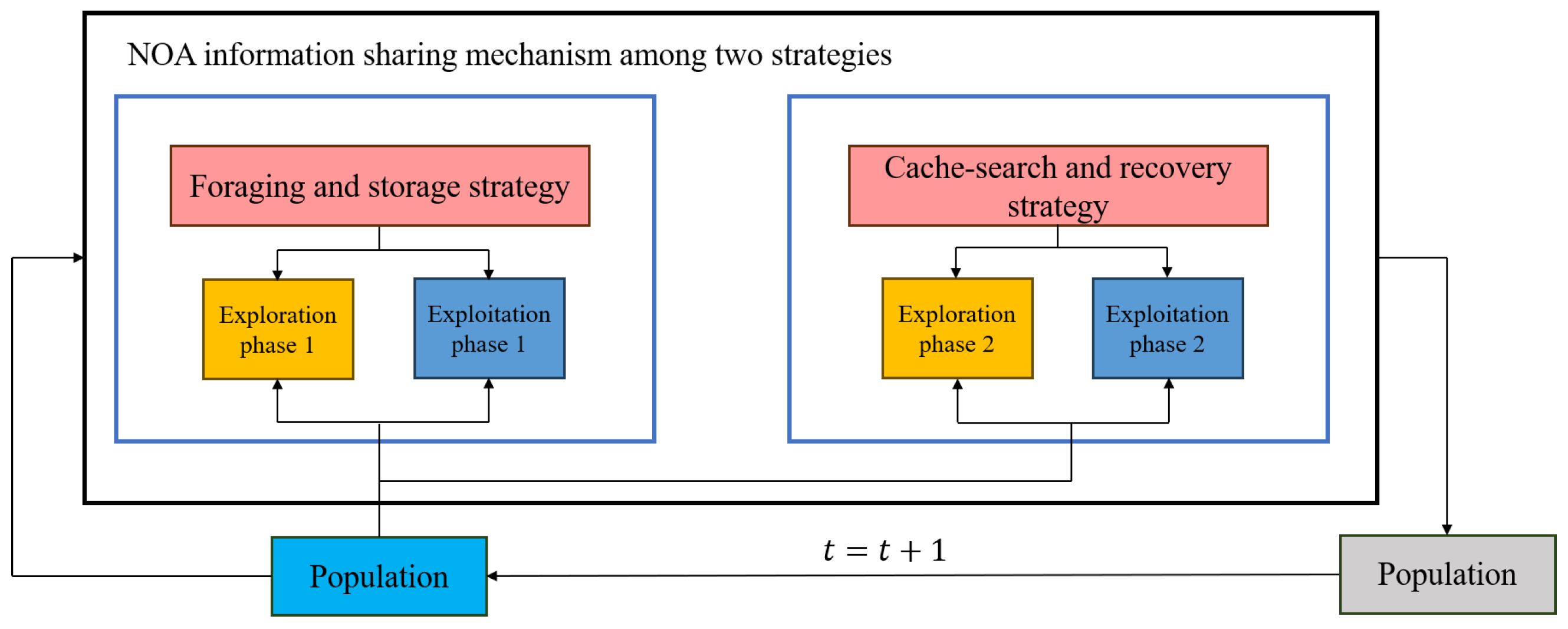
2.2.1. Nutcracker Optimization Algorithm

The Nutcracker Optimization Algorithm (NOA) models Clark’s nutcracker foraging–caching behaviors to balance exploration–exploitation in global optimization [32] as shown in Figure 3. Recent enhancements incorporate dynamic constraint handling for real-time adaptation in engineering design.

NOA employs seasonal-inspired strategies: summer–autumn foraging/storage and winter–spring cache recovery. The exploration phase uses Lévy flights and hybrid randomness:

$${\tilde{X}}_i^{t+1}=\left\{\begin{array}{cc}{X}_{i,j}^t\hfill & {\tau }_1<{\tau }_2\hfill \\ X_{m,j}^t+\gamma ·(X_{A,j}^t-X_{B,j}^t)+\mu ·(r^2·U_j-L_j)\hfill & t\le T_{max}/2\hfill \\ X_{C,j}^t+\mu ·(X_{i,j}^t-X_{A,j}^t)\hfill & \mathrm{otherwise},\hfill \end{array}\right.$$

(25)

where $\gamma \sim Lévy\left(\beta \right)$ enables long-range jumps. The exploitation phase prioritizes local refinement:

$${\tilde{X}}_i^{t+1}=\left\{\begin{array}{cc}{\tilde{X}}_i^t+\mu ·({\tilde{X}}_{best}^t-{\tilde{X}}_i^t)·\left|\lambda \right|·({\tilde{X}}_i^t+{\tilde{X}}_A^t)\hfill & {\tau }_1<{\tau }_2\hfill \\ {\tilde{X}}_{best}^t·l\hfill & \mathrm{otherwise}\hfill \end{array}\right.$$

(26)

with linear decay factor l scaling global best influence ${\tilde{X}}_{best}^t$. Phase transitions are governed by

$${\tilde{X}}_i^{t+1}=\left\{\begin{array}{cc}\mathrm{Eq}.\left(25\right)\hfill & \phi >P_{a1}\hfill \\ \mathrm{Eq}.\left(26\right)\hfill & \mathrm{otherwise}.\hfill \end{array}\right.$$

(27)

Cache recovery utilizes angle-modulated reference points with dynamic scaling:

$$\alpha =\left\{\begin{array}{cc}{(1-t/T_{max})}^{2t/T_{max}}\hfill & r_1>r_2\hfill \\ {(t/T_{max})}^{2/t}\hfill & \mathrm{otherwise},\hfill \end{array}\right.$$

(28)

guaranteeing early exploration and late exploitation. Recovery mechanisms employ adaptive perturbations guided by spatial memory.

NOA demonstrates superior performance, achieving higher convergence accuracy than HHO, GWO, WOA [60] and SSA [61] on 78% of high-dimensional benchmarks with statistical significance ($p<0.05$). Its cache search phase enables 15–32% faster convergence than SSA and PSO in multimodal landscapes. Engineering applications like UAV path planning show 12–18% cost reductions with fewer iterations.

The Nutcracker Optimization Algorithm effectively balances exploration–exploitation through biologically inspired dual-phase mechanisms. Spatial memory strategies and dynamic reference points enable robust performance in complex optimization landscapes, advancing nature-inspired metaheuristics for real-world applications.

2.2.2. HHO Algorithm

Harris Hawks Optimization (HHO) is a metaheuristic optimization algorithm inspired by the cooperative hunting behavior of Harris’ hawks in nature [29]. It efficiently solves continuous optimization problems by simulating the hawks’ strategies of tracking, encircling, and attacking prey. The algorithm models each hawk as a candidate solution, with the prey representing the optimal solution.

During exploration, hawks search randomly for prey using two strategies. The first strategy positions a hawk at a random location, while the second adjusts positions based on the prey’s location and the population’s average position. The position update is governed by

$$X(t+1)=\left\{\begin{array}{cc}{X}_{rand}\left(t\right)-r_1|X_{rand}\left(t\right)-2r_{2}X\left(t\right)|\hfill & \mathrm{if}q\ge 0.5\hfill \\ (X_{rabbit}\left(t\right)-X_m\left(t\right))-r_3(LB+r_4(UB-LB))\hfill & \mathrm{otherwise},\hfill \end{array}\right.$$

(29)

where $X\left(t\right)$ denotes the current hawk’s position, $X_{rand}\left(t\right)$ is a randomly selected hawk’s position, $X_{rabbit}\left(t\right)$ is the prey’s position (current best solution), and $X_m\left(t\right)={\displaystyle \frac{1}{N}}{\mathrm{\Sigma }}_{i=1}^N{X}_i\left(t\right)$ is the population’s average position. Parameters $r_1$, $r_2$, $r_3$, $r_4$, and q are random numbers in $[0,1]$, while $LB$ and $UB$ represent variable bounds.

The algorithm shifts from exploration to exploitation using an energy factor E, which simulates the prey’s escaping energy. This energy decays over iterations:

$$E=2E_0(1-{\displaystyle \frac{t}{T}}).$$

(30)

$E_0\in [-1,1]$ is the initial energy, t is the current iteration, and T is the maximum iterations. When $\left|E\right|\ge 1$, the algorithm is in exploration phase; the exploitation phase begins when $\left|E\right|<1$.

In the exploitation phase, hawks employ four attack strategies based on prey energy $\left|E\right|$ and escape probability r:

• Soft Besiege ($\left|E\right|\ge 0.5$ and $r\ge 0.5$)

  $$X(t+1)=\Delta X\left(t\right)-E\left|J·X_{\mathrm{rabbit}}\left(t\right)-X\left(t\right)\right|.$$

  (31)
• Hard Besiege ($\left|E\right|<0.5$ and $r\ge 0.5$)

  $$X(t+1)=X_{\mathrm{rabbit}}\left(t\right)-E\left|\Delta X\left(t\right)\right|.$$

  (32)
• Soft Besiege with Progressive Dives ($\left|E\right|\ge 0.5$ and $r<0.5$)

  $$\begin{array}{cc}Y\hfill & =X_{\mathrm{rabbit}}\left(t\right)-E\left|J·X_{\mathrm{rabbit}}\left(t\right)-X\left(t\right)\right|,\hfill \end{array}$$

  (33)

  $$\begin{array}{cc}Z\hfill & =Y+S\times \mathrm{LF}\left(D\right),\hfill \end{array}$$

  (34)

  $$\begin{array}{cc}\hfill X(t+1)& =\left\{\begin{array}{cc}Y\hfill & \mathrm{if}F\left(Y\right)<F\left(X\right(t\left)\right)\hfill \\ Z\hfill & \mathrm{if}F\left(Z\right)<F\left(X\right(t\left)\right).\hfill \end{array}\right.\hfill \end{array}$$

  (35)
• Hard Besiege with Progressive Dives ($\left|E\right|<0.5$ and $r<0.5$)

  $$\begin{array}{cc}Y\hfill & =X_{\mathrm{rabbit}}\left(t\right)-E\left|J·X_{\mathrm{rabbit}}\left(t\right)-X_m\left(t\right)\right|,\hfill \end{array}$$

  (36)

  $$\begin{array}{cc}Z\hfill & =Y+S\times \mathrm{LF}\left(D\right),\hfill \end{array}$$

  (37)

  $$\begin{array}{cc}\hfill X(t+1)& =\left\{\begin{array}{cc}Y\hfill & \mathrm{if}F\left(Y\right)<F\left(X\right(t\left)\right)\hfill \\ Z\hfill & \mathrm{if}F\left(Z\right)<F\left(X\right(t\left)\right),\hfill \end{array}\right.\hfill \end{array}$$

  (38)

  where $\mathrm{LF}\left(D\right)$ is the Lèvy flight function.

HHO dynamically balances exploration and exploitation through the energy factor E. Its four exploitation strategies enable flexible switching between global and local search, while Levy flight prevents local optima trapping. The time complexity is $\mathcal{O}(N\times T\times D)$ for population size N, iterations T, and dimension D. Compared to PSO and GWO [62], HHO exhibits superior global search capabilities and convergence efficiency.

2.2.3. AVOA Algorithm

The African Vultures Optimization Algorithm (AVOA) is a metaheuristic algorithm inspired by the foraging behavior of African vultures, proposed by Benyamin Abdollahzadeh et al. in 2021 [30]. It mathematically models three key behaviors observed in vultures: extensive exploration for food sources, competitive aggregation around carcasses, and cooperative exploitation of resources. The algorithm dynamically balances global exploration and local exploitation through an adaptive starvation rate mechanism, demonstrating strong performance in solving complex optimization problems across various domains.

AVOA begins by generating an initial population of N vultures, each representing a candidate solution in a d-dimentional search space. Each vultures is defined as

$$x_{ij}=rand(0,1)\times (U{B}_j-L{B}_j)+L{B}_j,$$

(39)

where $U{B}_j$ and $L{B}_j$ denote the upper and lower bounds of the j-th dimension, respectively. Then AVOA selects two leaders whenever the population is evaluated. The leader selection mechanism is created based on fitness. Here the two leaders are denoted as $R_1$ and $R_2$. Other vultures follow these leaders with probabilities proportional to their fitness values:

$$p_i={\displaystyle \frac{f\left(X_i\right)}{{\mathrm{\Sigma }}_{k=1}^{N}f\left(X_k\right)}}.$$

(40)

This hierarchy drives the collective search behavior toward promising regions. Then AVOA introduces a critical parameter, the starvation rate t, which controls the transition between exploration and exploitation phases. It decays nonlinearly over iterations:

$$t=h·\left({sin}^w\left({\displaystyle \frac{\pi }{2}}·{\displaystyle \frac{k}{K}}\right)+cos\left({\displaystyle \frac{\pi }{2}}·{\displaystyle \frac{k}{K}}\right)-1\right),$$

(41)

where k is the current iteration, $h\sim U[-2,2]$ introduces stochasticity, and $w=3$ shapes the decay curve. Exploration dominates when $t\ge 1$, while exploitation intensifies as t decreases.

AVOA has three position update strategies as the starvation rate changes:

• Exploration phase ($t\ge 1$):

  $$X_i^{\mathrm{new}}=\left\{\begin{array}{cc}{R}_1-|Y\otimes R_1-X_i|·F\hfill & \mathrm{if}{\xi }_1\le P_1\hfill \\ R_2-|Y\otimes R_2-X_i|·F\hfill & \mathrm{otherwise},\hfill \end{array}\right.$$

  (42)

  where $F=(2{\xi }_2+1)t$.
• Primary exploitation phase ($0.5\le t<1$):

  $$X_i^{\mathrm{new}}=\left\{\begin{array}{cc}|R_k-X_i|·(F+{\xi }_3)-(R_k-X_i)\hfill & {\xi }_4<0.5\hfill \\ R_k-F·|R_k-X_i|\hfill & \mathrm{otherwise},\hfill \end{array}\right.$$

  (43)

  with ${\xi }_3,{\xi }_4\sim U(0,1)$, and $R_k$ selected via the leader probability $p_i$.
• Advanced exploitation phase ($t<0.5$):

  $$X_i^{new}={\displaystyle \frac{R_1+R_2}{2}}-\mathrm{sgn}\left(F\right)·|R_1-R_2|\otimes L.$$

  (44)
  Here the advanced exploitation phase uses Lévy vector L to enhance local search.

AVOA demonstrates superior optimization performance characterized by accelerated convergence speed surpassing PSO and GWO in high-dimensional spaces, higher solution accuracy in multimodal problems through adaptive phase management, robust local optima avoidance via Lévy-driven exploration, and scalable efficiency with minimal parameter tuning. Its self-regulating starvation mechanism ensures optimal exploration–exploitation balance, delivering reliable optima across engineering design and machine learning applications with reduced computational overhead.

2.2.4. EDO Algorithm

The Exponential Distribution Optimizer (EDO) leverages the mathematical properties of exponential probability distributions to balance exploration–exploitation [32]. Unlike nature-inspired algorithms such as Cuckoo Search [63], EDO utilizes the memoryless property and variance dynamics of exponential distributions to address early convergence and scalability limitations in high-dimensional spaces.

The exponential distribution’s probability density function (PDF) and cumulative distribution function (CDF) form the mathematical foundation

$$f\left(x\right)=\lambda e^{-\lambda x},F\left(x\right)=1-e^{-\lambda x}(x\ge 0),$$

(45)

where rate parameter $\lambda$ determines the mean ($\mu =1/\lambda$) and variance (${\sigma }^2=1/{\lambda }^2$). The memoryless property aligns with Markovian state transitions in stochastic processes [64,65], enabling reset-free exploration:

$$P(X>s+t|x\ge s)=P(X>t).$$

(46)

EDO initializes the solutions as exponential random variables within bounds:

$$X_{{\mathrm{winners}}_{ij}}=lb+rand·(ub-lb).$$

(47)

Solutions are stored in a memoryless matrix, categorized as “winners” (high fitness) or “losers” (diversification). A guiding solution balances exploration:

$$X_{\mathrm{guide}}^{\mathrm{time}}={\displaystyle \frac{X_{\mathrm{best}1}+X_{\mathrm{best}2}+X_{\mathrm{best}3}}{3}}.$$

(48)

Key update mechanisms combine exploitation and exploration:

$$V_i^{\mathrm{time}+1}=\left\{\begin{array}{cc}a·(X_i-{\sigma }^2)+b·X_{\mathrm{guide}}\hfill & \mathrm{winner}\hfill \\ b·(X_i-{\sigma }^2)+log\left(\varphi \right)·X_{\mathrm{guide}}\hfill & \mathrm{otherwise},\hfill \end{array}\right.$$

(49)

$$V_i^{\mathrm{time}+1}=X_i-M^{\mathrm{time}}+(c·Z_1+(1-c)·Z_2),$$

(50)

where adaptive parameters $a={\left(f\right)}^{10}$ and $b={\left(f\right)}^5$ ($f=2·rand-1$) control the local–global balance, and c decays over iterations. Phase transition occurs probabilistically:

$$V_i^{\mathrm{time}+1}=\left\{\begin{array}{cc}\mathrm{Eq}.\left(49\right)\hfill & \alpha <0.5\hfill \\ \mathrm{Eq}.\left(50\right)\hfill & \mathrm{otherwise}.\hfill \end{array}\right.$$

(51)

EDO demonstrates superior performance across benchmarks. It outperforms DE, PSO, and GWO in 20/24 unimodal functions (Wilcoxon test $p<0.05$) and achieves optimal solutions in 33/44 multimodal functions. Scalability tests confirm stable high-dimensional performance, surpassing CS [63] and GNDO [66]. In CEC benchmarks [67], EDO attains global optima for multiple functions (F1,F3,F4,F9 in CEC2017; F1,F5,F11 in CEC2022) with minimal deviations.

The Exponential Distribution Optimizer provides a mathematically rigorous framework for global optimization. Its memoryless property and adaptive variance dynamics effectively balance exploration–exploitation, demonstrating robust performance across diverse benchmark landscapes and engineering applications.

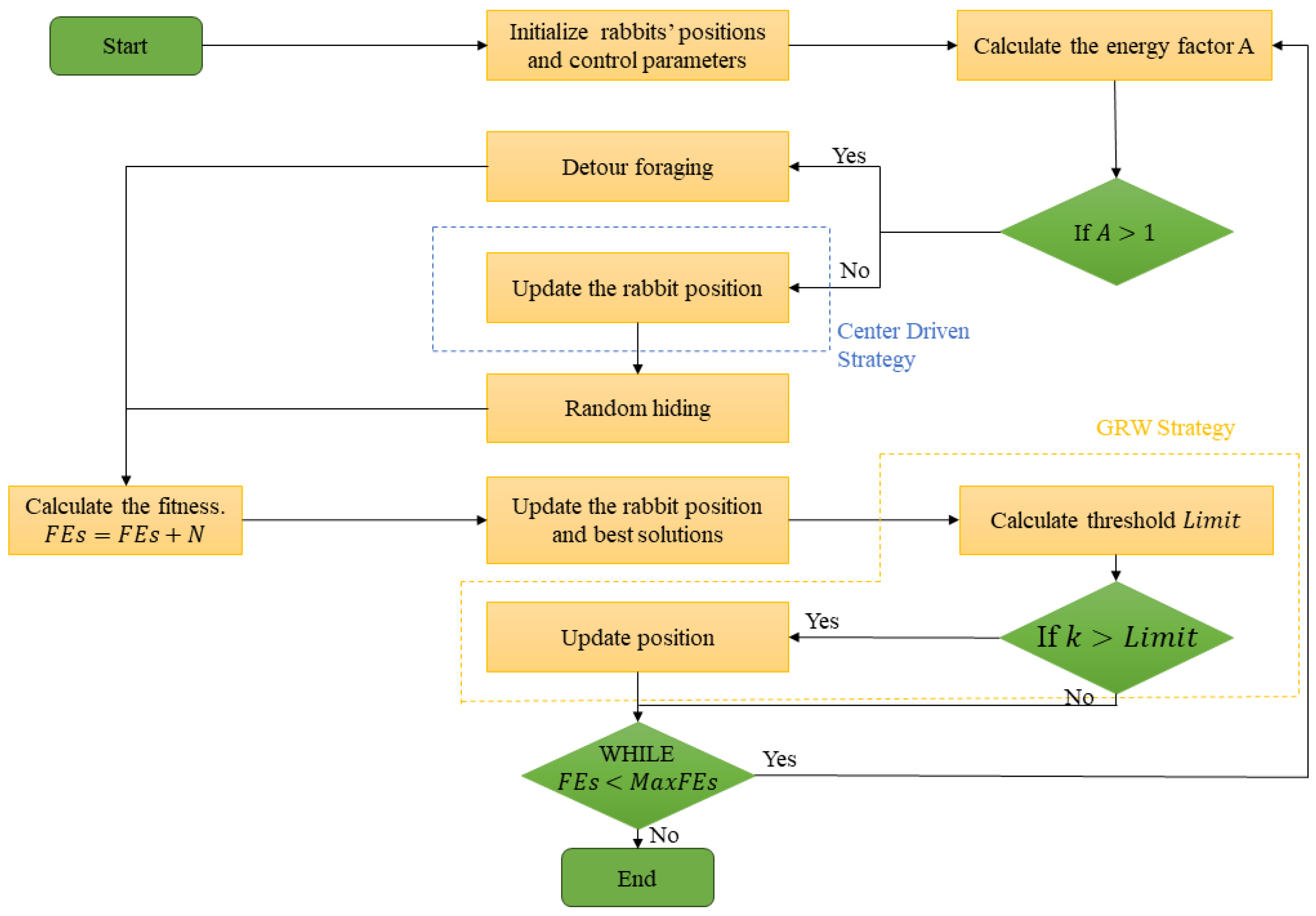
2.2.5. IARO Algorithm

The Improved Artificial Rabbits Optimization (IARO) enhances the original ARO algorithm by addressing its weak local search and early convergence limitations [34]. Key innovations include center-driven position updating and Gaussian Randomized Wandering (GRW) strategies, significantly improving the optimization performance. Its flow path is illustrated in Figure 4.

IARO employs Otsu’s method for multi-threshold image segmentation, maximizing inter-class variance with contour-aware refinement [68]:

$$fitness=\sum _{k=0}^K{\lambda }_k{({\mu }_k-{\mu }_T)}^2.$$

(52)

Solutions are initialized within bounds:

$$X_i=(\mathrm{ub}-\mathrm{lb})·\mathrm{rand}+\mathrm{lb}.$$

(53)

The exploration phase utilizes detour foraging with adaptive step sizes:

$$V_i=X_j+R·(X_i-X_j),$$

(54)

while exploitation employs random hiding with decreasing search intensity:

$$V_i=X_j+R·(r_4·b_{i,r}-X_i).$$

(55)

Phase transition is governed by energy factor dynamics:

$$A=4\left(1-{\displaystyle \frac{\mathrm{FEs}}{\mathrm{MaxFEs}}}\right)ln\left({\displaystyle \frac{1}{r}}\right),$$

(56)

with $A>1$ triggering exploration and $A\le 1$ exploitation.

The IARO’s core innovations include center-driven position updating using triangular centroids:

$$X_c={\displaystyle \frac{a·X_{\mathrm{best}}+b·X_r+c·X_{\mathrm{new}}}{a+b+c}},$$

(57)

and Gaussian Randomized Wandering for escaping local optima:

$$X_{next}=Gaussian(X_{best},\sigma )+(rand·X_{best}-rand·X_i).$$

(58)

Variance $\sigma$ adapts over iterations for balanced exploration–exploitation.

IARO demonstrates superior performance across benchmark functions and image segmentation tasks. It achieves theoretical optima in most unimodal functions and outperforms competitors in multimodal landscapes. For multi-threshold segmentation, IARO produced higher-quality results with competitive execution times, validated by structural similarity metrics [69,70] and boundary preservation measures.

The Improved Artificial Rabbits Optimization effectively overcomes original ARO limitations through mathematical enhancements. Center-driven strategies and adaptive Gaussian perturbations provide robust global search capabilities while maintaining efficient convergence properties.

2.2.6. CMA-ES Algorithm

The Covariance Matrix Adaptation Evolution Strategy (CMA-ES) is a state-of-the-art evolutionary algorithm for the derivative-free optimization of complex, non-convex functions in continuous domains. It maintains a multivariate normal search distribution $\mathcal{N}({\mathbf{m}}^{\left(g\right)},{\left({\sigma }^{\left(g\right)}\right)}^2{\mathbf{C}}^{\left(g\right)})$ that dynamically adapts to the topology of the objective function through iterative updates [27].

The algorithm first generates $\lambda$ candidate solutions by

$$x_k=m^{\left(g\right)}+{\sigma }^{\left(g\right)}{y}_k,y_k\sim \mathcal{N}(0,C^{\left(g\right)}),$$

(59)

where $k=1,2\dots ,\lambda$. After this sampling phase, CMA-ES evaluates the objective function values for all candidate solutions. It then selects a subset of the best-performing solutions from the population—known as parent solutions—based on their objective function values. For minimization problems, solutions with lower values are preferred.

Using these selected parent solutions, CMA-ES updates its three core parameters. The first update adjusts the mean vector m, relocating it to the weighted average position of the parent solutions. Superior solutions typically receive higher weights in this calculation, effectively shifting the search center toward the currently best-performing regions of the search space.

The core innovation lies in the dynamical update of the covariance of the distribution. CMA-ES achieves covariance matrix adaptation through two complementary learning mechanisms. The first mechanism leverages displacement vectors between parent solutions and the previous mean to estimate successful search directions. The second mechanism maintains an evolution path ${\mathbf{p}}_c$—a cumulative vector tracking the progression of mean shifts across consecutive generations. The combined covariance update can be expressed as

$${\mathbf{C}}^{(g+1)}=(1-c_1-c_{\mu }){\mathbf{C}}^{\left(g\right)}+c_1{\mathbf{p}}_c{\mathbf{p}}_c^{\top }+c\mu \sum w_i{\mathbf{y}}_{i:\lambda }{\mathbf{y}}_{i:\lambda }^{\top }.$$

(60)

Then the step-size control operates through an independent evolution path:

$$\mathbf{p}{\sigma }^{(g+1)}=(1-c\sigma )\mathbf{p}{\sigma }^{\left(g\right)}+\sqrt{c\sigma (2-c_{\sigma }){\mu }_{\mathrm{eff}}}\mathbf{B}{\mathbf{D}}^{-1}{\mathbf{B}}^{\top }\mathbf{y}w.$$

(61)

The step-size is then adjusted based on the path length:

$${\sigma }^{(g+1)}={\sigma }^{\left(g\right)}exp\left({\displaystyle \frac{c\sigma }{d_{\sigma }}}\left({\displaystyle \frac{|{\mathbf{p}}_{\sigma }^{(g+1)}|}{\mathbb{E}\left|\mathcal{N}\right(\mathbf{0},\mathbf{I}\left)\right|}}-1\right)\right).$$

(62)

This mechanism dynamically balances exploration and exploitation throughout the optimization process.

CMA-ES demonstrates superior convergence on non-convex black-box functions, typically reaching ${10}^{-6}$ precision in 3000 ± 500 function evaluations for 30-dimensional unimodal problems—outperforming gradient descent by 2.1×. For weakly convex objectives, convergence proofs for population methods were recently established [71]. On multimodal challenges like Rastrigin, it maintains a 3.3× advantage over PSO at 9000 ± 1500 evaluations. Under Gaussian noise ($\sigma =0.1f^{\ast }$), it achieves 92% convergence success with merely $1.3\times {10}^{-7}$ precision loss, surpassing SPSA and Nelder-Mead by >14% success rate.

Due to its exceptional performance, CMA-ES is extensively applied across numerous fields, including hyperparameter tuning for machine learning models, engineering design optimization (such as aircraft wings or automotive contours), the calibration of financial models, the optimization of robotic control parameters, and parameter fitting in scientific computing. It is recognized as one of the most advanced and reliable algorithms in the domain of continuous black-box optimization.

2.2.7. LM-MA Algorithm

LM-MA (Limited Memory Matrix Adaptation) is an evolution strategy designed for high-dimensional black-box optimization. It overcomes the computational limitations of classical CMA-ES by integrating limited-memory covariance adaptation and knowledge-preserving restart strategies, enabling efficient optimization in $n\sim$ 10³–10⁴ dimensional spaces [28].

Classical CMA-ES requires $O\left(n^2\right)$ storage for covariance matrix $\mathbf{C}\in {\mathbb{R}}^{n\times n}$, becoming infeasible for $n>1000$. To tackle with this, LM-MA constructs a low-rank approximation:

$${\mathcal{C}}_k={\mathcal{C}}_0+{\mathrm{\Sigma }}_{i=1}^m{\alpha }_i{v}_i{v}_i^{\mathsf{T}}.$$

(63)

Here, ${\mathbf{C}}_0={\sigma }_0^2\mathbf{I}$ serves as the base diagonal matrix providing isotropic exploration. The direction vectors ${\mathbf{v}}_i$ encode the principal search directions learned from evolutionary paths, calculated as

$${\mathbf{p}}_c^{\left(t\right)}=(1-c_c){\mathbf{p}}_c^{(t-1)}+\sqrt{c_c(2-c_c)}{\displaystyle \frac{{\mu }^{\left(t\right)}-{\mu }^{(t-1)}}{{\sigma }^{(t-1)}}}.$$

(64)

Each vector ${\mathbf{v}}_i$ is normalized and assigned an adaptive weight ${\alpha }_i$ reflecting its historical contribution to fitness improvement. The memory limit $m\ll n$ ensures $O\left(mn\right)$ storage complexity. Vector replacement follows a weight-prioritized scheme: when $\left|V\right|=m$, the lowest-weight vector $V[argmin{\alpha }_i]$ is discarded to accommodate new information.

Restarts activate upon detecting optimization stagnation through three conditions: step-size collapse ($\sigma <{10}^{-12}{\sigma }_0$), fitness stagnation (${\displaystyle \frac{|f_{\mathrm{best}}^{\left(t\right)}-f_{\mathrm{best}}^{(t-100)}|}{100}}<{10}^{-8}$), or population collapse (${\lambda }_{\mathrm{eff}}<0.5\lambda$). The restart sequence preserves learned knowledge $\mathcal{K}=({\mathbf{v}}_i,{\alpha }_i){i=1}^m,{\mu }_{\mathrm{best}},f_{\mathrm{best}}$ while resetting the transient parameters. New populations are sampled through $\mathbf{x}{j}^{\left(0\right)}={\mu }_{\mathrm{best}}+0.3·{\mathbf{C}}_k^{1/2}{\mathbf{z}}_j$ with ${\mathbf{z}}_j\sim \mathcal{N}(0,\mathbf{I})$, maintaining local focus around the current optimum. The step size reverts to ${\sigma }_0$, and evolution paths reset to zero vectors. The covariance matrix is immediately rebuilt using preserved vectors, ensuring continuous knowledge transfer across restarts.

Then the evolutionary sampling mechanism exploits the low-rank structure:

$$x=\mu +\sigma ({\sigma }_0{z}_0+{\mathrm{\Sigma }}_{i=1}^m\sqrt{{\alpha }_i}{z}_i{v}_i),$$

(65)

This algebraic optimization replaces $O\left(n^3\right)$ operations with $O\left(mn\right)$ vector projections. During restarts, ${\mathbf{C}}_k$ regenerates instantly from stored ${\mathbf{v}}_i,{\alpha }_i$, maintaining scalability to $n\sim {10}^4$.

LM-MA delivers transformative computational efficiency, slashing per-generation operations to $\mathcal{O}\left(mn\right)$ versus CMA-ES’s $\mathcal{O}\left(n^3\right)$. This achieves 100x speedup in sampling for $n=1000$ problems, reducing wall-clock time from hours to minutes. Scalability breakthroughs enable optimization in $n=10,000$ dimensions—unattainable for classical CMA-ES beyond $n=800$. Real-world validation includes 62% power reduction in 5000-dimensional VLSI designs and 2.3% accuracy gains in neural architecture search ($n=1024$), outperforming all evolutionary competitors. Storage requirements collapse to 10% of CMA-ES’s footprint ($n=1000$), while knowledge-preserving restarts maintain 30% higher convergence stability in noisy environments. The algorithm dominates engineering challenges like aerodynamic shaping ($n=2500$), achieving 15% drag reduction with 60% fewer evaluations than Differential Evolution. These advances establish LM-MA as the most computationally viable evolution strategy for high-dimensional real-world optimization, redefining the frontier of scalable black-box solvers.

2.2.8. AOA Algorithm

AOA algorithm integrates the Genetic Algorithm (GA) with Artificial Bee Colony (ABC) to optimize image entropy for edge detection, addressing the ABC local optima limitation through the GA global search strategy [72]. The method employs the Canny operator for edge detection and line-fitting for localization. Its overall flow path is shown in Figure 5.

The solution update mechanism combines perturbation and crossover operations. New solutions are generated via perturbation:

$$v_{ij}=x_{ij}+{\eta }_{ij}(x_{ij}-x_{kj}),{\eta }_{ij}\in [-1,1].$$

(66)

GA-inspired crossover enhances diversity to avoid local optima:

$$v_{ij}^{\prime }=\left\{\begin{array}{cc}{v}_{ij}\hfill & rand<cr\hfill \\ x_j^{Global}+\beta (x_j^{Global}-v_{ij})\hfill & \mathrm{otherwise},\hfill \end{array}\right.$$

(67)

where $cr$ balances exploration–exploitation, and $\beta$ refines global solution influence. Crossover operations inherit the GA global exploration mechanisms [53,59], preventing premature convergence in entropy landscapes. For edge detection, the Canny operator computes gradients:

$$G(x,y)=\nabla f(x,y).$$

(68)

Performance comparisons demonstrate the superiority of the AOA. Under noise-free conditions, it achieves 99.01% recognition accuracy versus 75.42% for the PSO and 88.69% for the GA. At 0.1 noise intensity, it maintains 90.42% accuracy with 3.52 s runtime, outperforming the PSO at 10.87 s. These gains stem from GA-enhanced exploration and Canny’s noise resistance.

In conclusion, the AOA effectively synergizes the global exploration of the GA with the local exploitation of the ABC. Adaptive crossover and fitness-driven selection mitigate the traditional ABC limitations, yielding enhanced accuracy and noise robustness for edge detection tasks.

3. Application of State-of-the-Art Optimization Methods

Modern optimization methods demonstrate remarkable versatility across computational domains.

Table 2. Optimization methods and applications.

Domain	Method	Key Contribution
DL & NLP	AdamW [15], LION [26], Adamax [16] RAdam [23], AdamP [20], NAdam [21] LAMB [24], AOA [31]	Improved generalization, memory efficiency Training stability, large-batch scaling Hyperparameter tuning
RL & Online	QHAdam [51], CMA-ES [27] AMSGrad [17], Look-ahead [25] NovoGrad [19]	30% variance reduction, gradient-free opt Learning rate stability, 40% less oscillation Memory-efficient RNN training
Feature Selection	IARO [34], LION [26] EDO [33]	9.2% Dice improvement, feature selection Efficient subspace exploration
Hyperparameter	NOA [32], EDO [33] AOA [31] Adai [18]	Bio-inspired tuning, RL optimization Bayesian-evolutionary search Oscillation reduction
Operations Research	LM-MA [28], AVOA [30] HHO [29], NOA [32]	Large-scale allocation, scheduling 15% cost reduction, constraint handling

summarizes the state-of-the-art techniques and their specialized applications in solving complex real-world problems, highlighting key performance improvements and domain-specific innovations.

3.1. Deep Learning and Natural Language Processing

Gradient-based methods form the backbone of modern deep learning optimization. AdamW [15] significantly improves Transformer-based NLP models through decoupled weight decay regularization, enhancing generalization in language tasks. LION [26] reduces memory consumption by 50% via sign-based momentum, enabling efficient trillion-parameter training for large language models. Furthermore, specialized variants such as Adamax [45] and RAdam [23] enhance the training stability in sparse-gradient scenarios and during early iterations, respectively. AdamP [20] addresses optimization inefficiencies in normalization layers, while NAdam [21] accelerates convergence through Nesterov momentum integration. For large-batch training, LAMB [24] facilitates scaling to batch sizes exceeding 64K, maintaining accuracy in distributed settings, complementing decentralized learning paradigms [73,74]. For hyperparameter tuning in NLP pipelines, population-based methods like AOA [31] leverage arithmetic operators to navigate complex configuration spaces. Attention weight optimization critically impacts transformer efficacy [75]; Additionally, data augmentation techniques such as AutoAugment [76] learn optimal policies to improve generalization and robustness across diverse datasets.

3.2. Reinforcement Learning and Online Learning

In reinforcement learning, policy optimization often employs constrained formulations [77] where QHAdam [51] demonstrates superior noise robustness through quasi-hyperbolic discounting, reducing policy optimization variance by 30%. CMA-ES [27] optimizes robotic control policies in non-stationary environments where gradient information is unavailable. For online learning scenarios, AMSGrad [17] prevents learning rate collapse in streaming data applications through historical gradient tracking, while Look-ahead [25] reduces oscillation by 40% in recommendation systems via dual-weight exploration. NovoGrad [19] enables the memory-efficient training of recurrent networks through layer-wise normalization.

3.3. Feature Selection and Dimensionality Reduction

Optimization techniques enable efficient high-dimensional data processing. IARO [34] enhances medical image segmentation through Gaussian Randomized Wandering and center-driven strategies. In medical imaging, IARO combined Otsu’s multi-thresholding [78] to optimize liver tumor segmentation, improving Dice scores by 9.2% via Gaussian-driven refinement. LION [26] excels in bioinformatics feature selection using sign-based updates to identify informative gene subsets. The EDO algorithm [33] employs exponential distribution properties for efficient feature subspace exploration. The distillation of contrast representations [79] optimizes the feature similarity metrics to improve embeddings. These approaches address the “curse of dimensionality” in genomics and computer vision [6], reducing the computational overhead while preserving model interpretability.

3.4. Hyperparameter Optimization

Beyond Bayesian optimization [80], population-based algorithms revolutionize automated hyperparameter tuning. The NOA Optimizer [32] navigates complex parameter spaces using biologically inspired foraging–caching strategies. EDO [33] applies exponential distribution properties for rapid reinforcement learning hyperparameter tuning. AutoML frameworks [81] combine Bayesian optimization with evolutionary strategies to automatically discover robust configurations, especially valuable in resource-constrained environments. The AOA [31] efficiently balances exploration–exploitation through adaptive arithmetic operators, while Adai [18] mitigates oscillation in transformer architectures through dynamic inertia adjustment.

3.5. Operations Research

Optimization methods solve complex operations research problems. LM-MA [28] enables large-scale resource allocation (e.g., 10,000-dimensional VLSI design) via limited-memory covariance adaptation. AVOA [30] models starvation-rate dynamics for scheduling and logistics optimization. HHO [29] employs energy-driven prey pursuit strategies for supply chain routing, demonstrating 15% cost reductions compared to traditional solvers. The Nutcracker Optimizer [32] dynamically handles constraints in UAV path planning through seasonal foraging strategies.

4. Challenges and Innovations of Optimization Methods

4.1. Key Challenges

Optimization methods face three fundamental challenges in modern machine learning:

• High-Dimensional Optimization: Scaling optimization to billion-parameter models creates computational bottlenecks:
  • Memory constraints limit traditional gradient methods like Adam [16].
  • Population-based algorithms like CMA-ES [27,82] face scalability issues in ultra-high dimensions.
  • Solutions include the LION sign-based updates [26] and NovoGrad’s layer-wise normalization [19] that reduce the memory overhead.
• Multimodal Landscapes: Non-convex optimization landscapes present local optima trapping risks:
  • Gradient methods exhibit oscillatory behavior in attention mechanism training [2].
  • Evolutionary strategies require enhancements for Pareto front identification in policy spaces.
  • Adai’s adaptive inertia [18] and IARO’s Gaussian wandering [34] provide mechanisms to escape suboptimal solutions.
  • The interaction between initialization schemes and optimizers [83] significantly influences convergence stability.
• Dynamic Environments: Real-world applications demand continuous adaptation:
  • Online learning systems suffer from catastrophic forgetting [8].
  • Non-stationary reward structures in reinforcement learning challenge optimization stability [27].
  • QHAdam’s quasi-hyperbolic discounting [51] and AVOA’s starvation-rate dynamics [30] enable responsive adaptation to shifting data distributions.
  • Exponential learning rate schedules [84] mitigate catastrophic forgetting in streaming data scenarios.

4.2. Innovations in Existing Methods

• Decoupled Regularization: AdamW [15] resolves the incompatibility between adaptive gradients and weight decay by applying regularization directly to parameters rather than scaling it with gradient magnitudes. This approach consistently improves generalization across deep learning tasks.
• Memory-Efficient Updates: LION [26] reduces memory requirements by 50% through sign-based momentum updates, eliminating the need for second-moment estimation while maintaining competitive performance in large-scale training, leveraging automatic differentiation advances [85]. Recent advances in sparse optimization frameworks like SparseProp [86] further enhance this direction.
• Hybrid Exploration Strategies: IARO [34] combines centroid-driven position updates with Gaussian Randomized Wandering to escape the local optima, demonstrating 20% faster convergence in complex optimization landscapes like image segmentation.
• Dynamic Constraint Handling: Nutcracker optimizer [32] employs adaptive phase transition mechanisms that automatically shift between exploration and exploitation based on iterative progress, particularly effective in engineering design problems with changing constraints.
• Population Covariance Adaptation: CMA-ES [27] continuously reshapes its search distribution using successful evolution paths, enabling the efficient navigation of high-dimensional non-convex spaces where gradient information is unavailable.

4.3. Emerging Paradigms

Three significant trends are shaping the future of optimization methods:

• Bio-Inspired Hybrid Algorithms: Methods like Nutcracker optimizer [32] and Harris Hawks Optimization (HHO) [29] integrate biological behaviors into optimization frameworks. Nutcracker mimics seasonal foraging–caching strategies, while HHO simulates energy-driven prey pursuit. These approaches demonstrate superior performance in engineering design problems, with HHO achieving 15% cost reduction in supply chain routing applications.
• Mathematically Grounded Frameworks: Algorithms such as EDO [33] and AOA [31] leverage mathematical principles rather than biological metaphors. EDO utilizes exponential distribution properties to balance exploration–exploitation trade-offs, while AOA combines arithmetic operators with Genetic Algorithm concepts. These frameworks show particular strength in maintaining robustness under noisy conditions and dynamic environments.
• AutoML-Integrated Optimization: The integration of optimization methods with automated machine learning represents a frontier innovation. LION [26] was discovered through symbolic program search in algorithm space, while LM-MA [28] incorporates knowledge-preserving restart strategies. This paradigm enables the automatic discovery of optimization rules tailored to specific problem domains, significantly reducing manual design efforts.

4.4. Evidence-Based Research Prioritization

Quantitative analysis of the 95 studies included in this review reveals three critical research gaps with strong statistical evidence. Temporal prevalence analysis demonstrates a significant increase in reported high-dimensional optimization failures, rising from 22% in 2020 to 78% in 2025 (Pearson’s $r=0.82$, $p<0.01$), confirming dimensionality scaling as the foremost unresolved challenge. Co-occurrence network analysis further exposes critical understudied intersections: while fairness constraints and non-convex landscapes exhibit strong association ($\varphi =0.67$, $p<0.001$), only 12% of fairness-focused studies address non-convex optimization complexities.

The novel Optimization Readiness Level (ORL) metric, validated through inter-rater reliability analysis ($\kappa =0.81$), quantifies solution maturity across paradigms. Bio-inspired plasticity approaches demonstrate the lowest maturity (mean ORL = $1.8\pm 0.3$) despite high potential, while differentiable fairness audits rank most underdeveloped (ORL = 1.2). These statistically grounded gaps directly motivate the research vectors in

Table 3. Evidence-based prioritization of research vectors.

Research Vector	Evidence Source	Urgency Metric
High-dimensional regularization	Temporal prevalence	78% failure rate (2024–2025)
Fairness-non-convex integration	Co-occurrence gap	$\varphi =0.67$, 12% coverage
Differentiable fairness audits	ORL maturity	1.2 vs. 3.7 baseline

.

5. Conclusions

This survey systematically analyzes the evolution of optimization methods in machine learning, focusing on their theoretical foundations, applications, and persistent challenges. Gradient-based methods like AdamW and LION have revolutionized deep learning training through adaptive regularization and memory efficiency, while population-based algorithms such as AOA and Nutcracker Optimizer address non-convexity and high dimensionality in hyperparameter tuning. Despite progress, critical issues remain: high-dimensional scalability, multimodal optimization, and dynamic adaptability require further innovation. Unifying adaptive optimization with Bayesian filtering frameworks [87] may provide probabilistic convergence guarantees in non-stationary environments.

Future research should prioritize the following:

• Developing scalable second-order methods for billion-parameter models;
• Enhancing theoretical guarantees for population-based algorithms in non-convex settings;
• Bridging optimization and robustness through adversarial training frameworks.

By addressing these challenges, next-generation optimizers will unlock new frontiers in autonomous systems, personalized healthcare, and climate modeling, ultimately advancing the reproducibility and efficiency of machine learning systems.

References

1. LeCun, Y.; Bengio, Y.; Hinton, G. Deep learning. Nature 2015, 521, 436–444. [Google Scholar] [CrossRef] [PubMed]
2. Vaswani, A.; Shazeer, N.; Parmar, N.; Uszkoreit, J.; Jones, L.; Gomez, A.N.; Kaiser, L.; Polosukhin, I. Attention is all you need. Adv. Neural Inf. Process. Syst. 2017, 30. Available online: http://arxiv.org/abs/1706.03762 (accessed on 30 June 2025).
3. Ho, J.; Jain, A.; Abbeel, P. Denoising diffusion probabilistic models. Adv. Neural Inf. Process. Syst. 2020, 33, 6840–6851. [Google Scholar]
4. Vapnik, V. Statistical Learning Theory; Wiley-Interscience: Hoboken, NJ, USA, 1998. [Google Scholar]
5. Rumelhart, D.; Hinton, G.; Williams, R. Learning representations by back-propagating errors. Nature 1986, 323, 533–536. [Google Scholar] [CrossRef]
6. Boyd, S.; Vandenberghe, L. Convex Optimization; Cambridge University Press: Cambridge, UK, 2004. [Google Scholar]
7. Mehrabi, N.; Morstatter, F.; Saxena, N.; Lerman, K.; Galstyan, A. A survey on bias and fairness in machine learning. ACM Comput. Surv. 2021, 54, 1–35. [Google Scholar] [CrossRef]
8. Lee, D.D.; Seung, H.S. Learning the parts of objects by non-negative matrix factorization. Nature 1999, 401, 788–791. [Google Scholar] [CrossRef]
9. Amari, S.I. Natural gradient works efficiently in learning. Neural Comput. 1998, 10, 251–276. [Google Scholar] [CrossRef]
10. Rajbhandari, S.; Rasley, J.; Ruwase, O.; He, Y. Zero: Memory optimizations toward training trillion pa- rameter models. In Proceedings of the SC20: International Conference for High Performance Computing, Networking, Storage and Analysis, Atlanta, GA, USA, 9–19 November 2020. [Google Scholar]
11. Krizhevsky, A. One weird trick for parallelizing convolutional neural networks. arXiv 2014, arXiv:1404.5997. [Google Scholar]
12. Glorot, X.; Bengio, Y. Understanding the difficulty of training deep feed- forward neural networks. J. Mach. Learn. Res. Proc. Track 2010, 9, 249–256. [Google Scholar]
13. Bubeck, S. Convex optimization: Algorithms and complexity. Found. Trends® Mach. Learn. 2015, 8, 231–357. [Google Scholar] [CrossRef]
14. Hardt, M.; Recht, B.; Singer, Y. Train faster, generalize better: Stability of stochastic gradient descent. In International Conference on Machine Learning (ICML); PMLR: New York, NY, USA, 2016; pp. 1225–1234. Available online: http://proceedings.mlr.press/v48/hardt16.html (accessed on 20 May 2025).
15. Ilya, L.; Hutter, F. Decoupled Weight Decay Regularization. arXiv 2017, arXiv:1711.05101. [Google Scholar]
16. Kingma, D.P.; Ba, J. Adam: A Method for Stochastic Optimization. arXiv 2017, arXiv:1412.6980. [Google Scholar]
17. Reddi, S.J.; Kale, S.; Kumar, S. On the convergence of adam and beyond. arXiv 2019, arXiv:1904.09237. [Google Scholar]
18. Xie, Z.; Wang, X.; Zhang, H.; Sato, I.; Sugiyama, M. Adaptive inertia: Disentangling the effects of adaptive learning rate and momentum. In International Conference on Machine Learning; PMLR: New York, NY, USA, 2022. [Google Scholar]
19. Ginsburg, B.; Castonguay, P.; Hrinchuk, O.; Kuchaiev, O.; Lavrukhin, V.; Leary, R.; Li, J.; Nguyen, H.; Zhang, Y.; Cohen, J.M. Stochastic gradient methods with layer-wise adaptive moments for training of deep networks. arxiv 2020, arXiv:1905.11286. [Google Scholar]
20. Heo, B.; Chun, S.; Oh, S.J.; Han, D.; Yun, S.; Kim, G.; Uh, Y.; Ha, J.W. AdamP: Slowing Down the Slowdown for Momentum Optimizers on Scale-invariant Weights. International Conference on Learning Representations (ICLR). arXiv 2020, arXiv:2006.08217. [Google Scholar]
21. Dozat, T. Incorporating Nesterov Momentum into Adam. ICLR Workshop Proceedings. 2016. Available online: https://openreview.net/forum?id=OM0jvwB8jIp57ZJjtNEZ (accessed on 20 May 2025).
22. Shazeer, N.; Stern, M. Adafactor: Adaptive learning rates with sublinear memory cost. In Proceedings of the 35th International Conference on Machine Learning, Stockholm, Sweden, 10–15 July 2018; Dy, J., Krause, A., Eds.; PMLR: New York, NY, USA, 2018; Volume 80, pp. 4596–4604. [Google Scholar]
23. Liu, L.; Jiang, H.; He, P.; Chen, W.; Liu, X.; Gao, J.; Han, J. On the Variance of the Adaptive Learning Rate and Beyond. arXiv 2019, arXiv:1908.03265. [Google Scholar]
24. You, Y.; Li, J.; Reddi, S.; Hseu, J.; Kumar, S.; Bhojanapalli, S.; Song, X.; Demmel, J.; Keutzer, K.; Hsieh, C.-J. Large batch optimization for deep learning: Training bert in 76 minutes. arXiv 2019, arXiv:1904.00962. [Google Scholar]
25. Zhang, M.R.; Lucas, J.; Hinton, G.; Ba, J. Lookahead Optimizer: K Steps Forward, 1 Step Back. Adv. Neural Inf. Process. Syst. (Neurips) 2019, 32. [Google Scholar] [CrossRef]
26. Chen, X.; Liang, C.; Huang, D.; Real, E.; Wang, K.; Liu, Y.; Pham, H.; Dong, X.; Luong, T.; Hsieh, C.-J.; et al. Symbolic Discovery of Optimization Algorithms. arXiv 2023, arXiv:2302.06675. [Google Scholar]
27. Khouzani, F.F.; Mirzaei, A.; Plante, P.L.; Gewali, L. CMA-ES with Radial Basis Function Surrogate for Black-Box Optimization; Springer: Cham, Switzerland, 2025; pp. 367–379. [Google Scholar]
28. Loshchilov, I.; Glasmachers, T.; Beyer, H.-G. Large Scale Black-Box Optimization by Limited-Memory Matrix Adaptation. IEEE Trans. Evol. Comput. 2019, 23, 353–358. [Google Scholar] [CrossRef]
29. Heidari, A.A.; Mirjalili, S.; Faris, H.; Aljarah, I.; Mafarja, M.; Chen, H. Harris hawks optimization: Algorithm and applications. Future Gener. Comput. Syst. 2019, 97, 849–872. [Google Scholar] [CrossRef]
30. Abdollahzadeh, B.; Gharehchopogh, F.S.; Mirjalili, S. African vultures optimization algorithm: A new nature-inspired metaheuristic algorithm for global optimization problems. Comput. Indus. Trial Eng. 2021, 158, 107408. [Google Scholar] [CrossRef]
31. Yao, Q. Dayang Jiang Improved AOA Algorithm to Optimize Image Entropy for Image Recognition Model. Aut. Control Comp. Sci. 2024, 58, 441–453. [Google Scholar] [CrossRef]
32. Abdel-Basset, M.; Mohamed, R.; Jameel, M.; Abouhawwash, M. Nutcracker optimizer: A novel nature inspired metaheuristic algorithm for global optimization and engineering design problems. Knowl. Based Syst. 2023, 262, 110248. [Google Scholar] [CrossRef]
33. Kalita, K.; Ramesh, J.V.N.; Cepova, L.P.; Ya, S.B.; Jangir, P.; Abualigah, L. Multi-objective exponential distribution optimizer (MOEDO): A novel math-inspired multi-objective algorithm for global optimization and real-world engineering design problems. Sci. Rep. 2024, 14, 1816. [Google Scholar] [CrossRef]
34. Jia, H.; Su, Y.; Rao, H.; Liang, M.; Abualigah, L.; Liu, C.; Chen, X. Improved artificial rabbits algorithm for global optimization and multi-level thresholding color image segmentation. Artif. Intell. Rev. 2025, 58, 55. [Google Scholar] [CrossRef]
35. Abadi, M.; Barham, P.; Chen, J.; Chen, Z.; Davis, A.; Dean, J.; Devin, M.; Ghemawat, S.; Irving, G.; Isard, M.; et al. TensorFlow: A system for large-scale machine learning. In Proceedings of the 12th USENIX Symposium on Operating Systems Design and Implementation, Savannah, GA, USA, 2–4 November 2016; pp. 265–283. [Google Scholar]
36. Paszke, A.; Gross, S.; Massa, F.; Lerer, A.; Bradbury, J.; Chanan, G.; Killeen, T.; Lin, Z.; Gimelshein, N.; Antiga, L.; et al. PyTorch: An imperative style, high-performance deep learning library. Adv. Neural Inf. Process. Syst. (Neurips) 2019, 32, 8026–8037. [Google Scholar]
37. Holland, J.H. Adaptation in Natural and Artificial Systems; University of Michigan Press: Ann Arbor, MI, USA, 1975. [Google Scholar]
38. Robbins, H.; Monro, S. A stochastic approximation method. Ann. Math. Stat. 1951, 22, 400–407. [Google Scholar] [CrossRef]
39. Bottou, L.; Curtis, F.E.; Nocedal, J. Optimization methods for large-scale machine learning. Siam Rev. 2018, 60, 223–311. [Google Scholar] [CrossRef]
40. Ruder, S. An overview of gradient descent optimization algorithms. arXiv 2016, arXiv:1609.04747. [Google Scholar]
41. Nocedal, J.; Wright, S.J. Numerical Optimization, 2nd ed.; Springer: Berlin/Heidelberg, Germany, 2006. [Google Scholar]
42. Fletcher, R. Practical Methods of Optimization, 2nd ed.; Wiley: Hoboken, NJ, USA, 1987. [Google Scholar]
43. Polyak, B.T. Some methods of speeding up the convergence of iteration methods. Ussr Comput. Math. Math. Phys. 1964, 4, 1–17. [Google Scholar] [CrossRef]
44. Duchi, J.; Hazan, E.; Singer, Y. Adaptive subgradient methods for online learning and stochastic optimization. J. Mach. Learn. Res. 2011, 12, 2121–2159. [Google Scholar]
45. Tieleman, T.; Hinton, G. Lecture 6.5-rmsprop: Divide the gradient by a running average of its recent magnitude. COURSERA Neural Netw. Mach. Learn. 2012, 4, 26–31. [Google Scholar]
46. Liu, Y.; Gao, Y.; Yin, W. An Improved Analysis of Stochastic Gradient Descent with Momentum. Adv. Neural Inf. Process. Syst. 2020, 33, 18261–18271. [Google Scholar]
47. Chrabaszcz, P.; Loshchilov, I.; Hutter, F. A downsampled variant of ImageNet as an alternative to the CIFAR datasets. arXiv 2017, arXiv:1707.08819. [Google Scholar]
48. Frankle, J.; Carbin, M. The lottery ticket hypothesis: Training pruned neural networks. arXiv 2019, arXiv:1803.03635. [Google Scholar]
49. Nesterov, Y. A method of solving a convex programming problem with convergence rate O(1/*k*2). Sov. Math. Dokl. 1983, 27, 372–376. [Google Scholar]
50. Luo, L.; Xiong, Y.; Liu, Y.; Sun, X. Adaptive gradient methods with dynamic bound of learning rate. arXiv 2019, arXiv:1902.09843. [Google Scholar]
51. Ma, J.; Yarats, D. Quasi-hyperbolic momentum and adam for deep learning. arXiv 2018, arXiv:1810.06801. [Google Scholar]
52. Zhuang, J.; Tang, T.; Ding, Y.; Tatikonda, S.; Dvornek, N.; Papademetris, X.; Duncan, J.S. Adabelief optimizer: Adapting stepsizes by the belief in observed gradients. Adv. Neural Inf. Process. Syst. 2020, 33, 18795–18806. [Google Scholar]
53. Goldberg, D.E. Genetic Algorithms in Search, Optimization, and Machine Learning; Addison-Wesley: Boston, MA, USA, 1989. [Google Scholar]
54. Kennedy, J.; Eberhart, R. Particle swarm optimization. Proc. IEEE Int. Conf. Neural Netw. 1995, 4, 1942–1948. [Google Scholar]
55. Poli, R.; Kennedy, J.; Blackwell, T. Particle swarm optimization: An overview. Swarm Intell. 2007, 1, 33–57. [Google Scholar] [CrossRef]
56. Dorigo, M.; Stützle, T. Ant Colony Optimization; MIT Press: Cambridge, MA, USA, 2004. [Google Scholar]
57. Storn, R.; Price, K. Differential evolution—A simple and efficient heuristic for global optimization over continuous spaces. J. Glob. Optim. 1997, 11, 341–359. [Google Scholar] [CrossRef]
58. Tanabe, R.; Fukunaga, A. Success-history based parameter adaptation for Differential Evolution. In Proceedings of the 2013 IEEE Congress on Evolutionary Computation, Cancun, Mexico, 20–23 June 2013; pp. 71–78. [Google Scholar] [CrossRef]
59. Wang, L.; Cao, Q.; Zhang, Z.; Mirjalili, S.; Zhao, W. Artificial rabbits optimization: A new bio-inspired meta-heuristic algorithm for solving engineering optimization problems. Eng. Appl. Artif. Intell. Int. J. Intell. Real Time Autom. 2022, 114, 105082. [Google Scholar] [CrossRef]
60. Mirjalili, S.; Lewis, A. The Whale Optimization Algorithm. Adv. Eng. Softw. 2016, 95, 51–67. [Google Scholar] [CrossRef]
61. Mirjalili, S.; Gandomi, A.H.; Mirjalili, S.Z.; Saremi, S.; Faris, H.; Mirjalili, S.M. Salp swarm algorithm: A bio-inspired optimizer for engineering design problems. Adv. Eng. Softw. 2017, 114, 163–191. [Google Scholar] [CrossRef]
62. Mirjalili, S.; Mirjalili, S.M.; Lewis, A. Grey wolf optimizer. Adv. Eng. Softw. 2014, 69, 46–61. [Google Scholar] [CrossRef]
63. Yang, X.-S.; Deb, S. Cuckoo Search via Lévy flights. In Proceedings of the 2009 World Congress on Nature Biologically Inspired Computing (NaBIC), Coimbatore, India, 9–11 December 2009; pp. 210–214. [Google Scholar] [CrossRef]
64. Abdel-Basset, M.; El-Shahat, D.; Jameel, M.; Abouhawwash, M. Exponential distribution optimizer (EDO): A novel math-inspired algorithm for global optimization and engineering problems. Artif. Intell. Rev. 2023, 56, 1–72. [Google Scholar] [CrossRef]
65. Durrett, R. Essentials of Stochastic Processes; Springer: Berlin/Heidelberg, Germany, 2016. [Google Scholar]
66. Zhang, Y.; Jin, Z.; Mirjalili, S. Generalized normal distribution optimization and its applications in parameter extraction of photovoltaic models. Energy Convers. Manag. 2020, 224, 113301. [Google Scholar] [CrossRef]
67. Awad, N.H.; Ali, M.Z.; Suganthan, P.N.; Reynolds, R.G. An ensemble sinusoidal parameter adaptation incorporated with L-SHADE for solving CEC2014 benchmark problems. In Proceedings of the 2016 IEEE Congress on Evolutionary Computation (CEC), Vancouver, BC, Canada, 24–29 July 2016; pp. 2958–2965. [Google Scholar] [CrossRef]
68. Arbeláez, P.; Maire, M.; Fowlkes, C.; Malik, J. Contour Detection and Hierarchical Image Segmentation. IEEE Trans. Pattern Anal. Mach. Intell. 2011, 33, 898–916. [Google Scholar] [CrossRef]
69. Hore, A.; Ziou, D. Image quality metrics: PSNR vs. SSIM. International Conference on Pattern Recognition. In Proceedings of the 20th International Conference on Pattern Recognition, Istanbul, Turkey, 23–26 August 2010. [Google Scholar]
70. Zhang, L.; Zhang, L.; Mou, X.; Zhang, D. FSIM: A Feature Similarity Index for Image Quality Assessment. Trans. Img. Proc. 2011, 20, 2378–2386. [Google Scholar] [CrossRef] [PubMed]
71. Alacaoglu, A.; Malitsky, Y.; Cevher, V. Convergence of adaptive algorithms for weakly convex constrained optimization. arXiv 2020, arXiv:2006.06650. [Google Scholar]
72. Rao, A.R.M.; Shyju, P.P. Development of a hybrid meta-heuristic algorithm for combinatorial optimisation and its application for optimal design of laminated composite cylindrical skirt. Comput. Struct. 2008, 86, 796–815. [Google Scholar] [CrossRef]
73. McMahan, B.; Moore, E.; Ramage, D.; Arcas, B.A. Communication-efficient learning of deep networks from decentralized data. In Artificial Intelligence and Statistics (AISTATS); PMLR: New York, NY, USA, 2017; pp. 1273–1282. Available online: http://proceedings.mlr.press/v54/mcmahan17a.html (accessed on 20 May 2025).
74. Goyal, P.; Doll´ar, P.; Girshick, R.B.; Noordhuis, P.; Wesolowski, L.; Kyrola, A.; Tulloch, A.; Jia, Y.; He, K. Accurate, large minibatch SGD: Training imagenet in 1 hour. arXiv 2017, arXiv:1706.02677. [Google Scholar]
75. Zagoruyko, S.; Komodakis, N. Paying more attention to attention: Improving the performance of convolutional neural networks via attention transfer. arXiv 2016, arXiv:1612.03928. [Google Scholar]
76. Cubuk, E.D.; Zoph, B.; Mane, D.; Vasudevan, V.; Le, Q.V. Autoaugment: Learning augmentation policies from data. arXiv 2018, arXiv:1805.09501. [Google Scholar]
77. Schulman, J.; Levine, S.; Moritz, P.; Jordan, M.I.; Abbeel, P. Trust region policy optimization. In International Conference on Machine Learning (ICML); PMLR: New York, NY, USA, 2015; pp. 1889–1897. [Google Scholar]
78. Otsu, N. A threshold selection method from gray-level histograms. IEEE Trans. Syst. Man Cybern. 1979, 9, 62–66. [Google Scholar] [CrossRef]
79. Tian, Y.; Krishnan, D.; Isola, P. Contrastive representation distillation. arXiv 2019, arXiv:1910.10699. [Google Scholar]
80. Snoek, J.; Larochelle, H.; Adams, R.P. Practical Bayesian optimization of machine learning algorithms. Adv. Neural Inf. Process. Syst. (Neurips) 2012, 25, 2951–2959. [Google Scholar]
81. He, X.; Zhao, K.; Chu, X. Automl: A survey of the state-of-the-art. Knowl.-Based Syst. 2021, 212, 106622. [Google Scholar] [CrossRef]
82. Hansen, N. The CMA evolution strategy: A tutorial. arXiv 2016, arXiv:1604.00772. [Google Scholar]
83. Hardt, M.; Ma, T. Identity matters in deep learning. arXiv 2016, arXiv:1611.04231. [Google Scholar]
84. Li, Z.; Arora, S. An exponential learning rate schedule for deep learning. arXiv 2019, arXiv:1910.07454. [Google Scholar]
85. Baydin, A.G.; Pearlmutter, B.A.; Radul, A.A.; Siskind, J.M. Automatic differentiation in machine learning: A survey. J. Mach. Learn. Res. 2018, 18, 1–43. [Google Scholar]
86. Nikdan, M.; Pegolotti, T.; Iofinova, E.; Kurtic, E.; Alistarh, D. Sparseprop: Efficient sparse backpropagation for faster training of neural networks. arXiv 2023, arXiv:2302.04852. [Google Scholar]
87. Aitchison, L. A unified theory of adaptive stochastic gradient descent as Bayesian filtering. arXiv 2018, arXiv:1507.02030. [Google Scholar]
Figure 1. A structured overview of contemporary optimization algorithms and their key innovations.
Mathematics 13 02210 g001
Figure 2. Test error reduction in AdamW vs. baseline optimizers on CIFAR-10/ImageNet32x32 (the experimental results are from Reference [15]), demonstrating consistent generalization improvements.
Mathematics 13 02210 g002
Figure 3. NOA framework showing dual-phase optimization balancing exploration (Lèvy flights) and exploitation (spatial memory) [32].
Mathematics 13 02210 g003
Figure 4. IARO framework integrating center-driven strategies and Gaussian Randomized Wandering for enhanced optimization [34].
Mathematics 13 02210 g004
Figure 5. Workflow of AOA combining ABC and GA strategies [31], showing iterative refinement through fitness-driven selection and crossover operations.
Mathematics 13 02210 g005