Applications of the Calculus by the Transfer Matrix Method for Long Rectangular Plates Under Uniform Vertical Loads

Abstract

The aim of this work is to present an original, relatively simple, and elegant approach to the analysis of long rectangular plates subjected to uniformly distributed vertical loads acting on various surfaces. Plate analysis is important in many fields, especially where components are either rectangular plates or can be approximated as such. The Transfer Matrix Method is increasingly used in research, as evidenced by the references cited. The advantages of this method lie in the simplicity of its algorithm, the ease of implementation in programming, and its straightforward integration into optimization software. The approach consists of discretizing the rectangular plate by sectioning it with planes parallel to the short sides—i.e., perpendicular to the two long edges. This results in a set of beams, each with a length equal to the width of the plate, a height equal to the plate’s thickness, and a unit width. Each unit beam has support at its ends that replicate the edge conditions of the plate along its long sides. In the study presented, the rectangular plate is embedded along its two long edges, meaning the unit beam is considered embedded at both ends. The Transfer Matrix Method is particularly valuable because it lends itself well to iterative calculations, making it easy to develop software capable of analyzing long rectangular plates quickly. This makes it especially useful for shape optimization applications, which we intend and hope to pursue in future studies.

1. Introduction

This work presents plate calculus, which plays a significant role in various fields, particularly in industry, engineering, construction, and medicine, especially in orthodontics. The Transfer Matrix Method (TMM) offers an effective and appropriate approach for iterative calculations, which are essential for solving shape optimization problems. The approach presented in this work is original. The TMM is a mathematical technique used to analyze structures that can be discretized into elements, using an iterative process as described in [1], which outlines the fundamentals of structural analysis.

The classic calculus of Strength of Materials can be found in [2,3]. The calculus of long rectangular plates embedded at long borders with a uniform vertical load on a line parallel to the long borders through the TMM with applications in vehicle industry is given in [4]. The TMM calculus for a long cylinder tube with industrial applications can be seen in [5]. Applications of the TMM in other fields, for example, in Odontology, are presented in [6,7]. A triangular shell element for geometrically nonlinear analysis can be seen in [8]. The calculus of a long rectangle plate articulated on both long borders charged with a linear load uniformly distributed on a line parallel to the long borders through the TMM is given in [9]. A simple triangular finite element for nonlinear thin shells in statics, dynamics, and anisotropy is presented in [10], and a simple geometrically exact finite element for thin shells in statics can be shown in [11].

A meshless analysis of shear deformable shells with boundary and interface constraints is given in [12]. The Finite Elements Method (FEM) for calculus of rectangular plates is presented in [13,14]. The bending of rectangular plates with each arbitrary edge point supported under a concentrated load can be shown in [15]. An analysis of folded plate structures by a combined boundary element and TMM is given in [16]. An FEM and TMM for the dynamic analysis of frame structures is presented in [17]. An elastic analysis and application tables of rectangular plates with unilateral contact support conditions can be seen in [18]. Theoretical aspects for the time-harmonic analysis of acoustic pulsation in gas pipeline systems using the FEM and TMM are presented in [19].

An integrated TMM for multiply connected mufflers is given in [20]. The determination of the stress–strain state in thin orthotropic plates on Winkler’s elastic foundations is given in [21]. An evaluation of a hybrid underwater sound-absorbing meta-structure by using the TMM is presented in [22]. Some theoretical and experimental extensions based on the properties of the intrinsic transfer matrix can be found in [23]. The TMM applied to the parallel assembly of sound-absorbing materials is presented in [24]. The past, the present, and the future multibody system with the TMM is presented in [25]. The TMM for multibody systems (Rui method) and its applications are presented in [26]. Muffler modeling by the TMM and the experimental verification can be seen in [27].

The development of a two-dimensional theory of thick plates bending on the basis of the general solution of the Lamé equations is given in [28]. The coupling of the TMM with FEM for analyzing the acoustics of complex hollow body networks is presented in [29]. Equivalent systems for the analysis of rectangular plates of varying thickness can be seen in [30]. Elements of the classical theory of plates are presented in [31]. A study about the bending of clamped rectangular plates is given in [32]. The determination of plane stress–strain states of the plates on the basis of the three-dimensional theory of elasticity is given in [33]. An analysis of the hypotheses used when constructing the theory of beams and plates can be found in [34].

The calculus of plates by the series representation of the deflection function is presented in [35]. The solution of non-rectangular plates with the macro-element method is given in [36]. The stress state of a compound polygonal plate can be found in [37]. The solution to thin rectangular plates with various boundary conditions is given in [38]. An exact solution for the deflection of a clamped rectangular plate under a uniform load is given in [39]. The stress and strain state in the corner points of a clamped plate under a uniformly distributed normal load can be seen in [40]. A static analysis of an orthotropic plate is presented in [41]. The theory of plates and shells can be found in [42]. The stress and strain analysis of rectangular plates with a variable thickness and constant weight is presented in [43]. An analysis of homogeneous and non-homogeneous plates can be found in [44]. A theoretical and comparative study regarding the mechanical response under the static loading for different rectangular plates is presented in [45]. Approximate analytical solutions in the analysis of thin elastic plates can be shown in [46]. Some aspects of the implementation of the boundary elements method in plate theory are presented in [47].

A convergence analysis of the finite element approach to the classical approach for the analysis of plates in bending is given in [48]. The method of matched sections as a beam, like the approach for plate analysis, is given in [49]. The application of numerical methods in solving a phenomenon of the theory of thin plates can be seen in [50]. A review of a few selected theories of plates in bending is presented in [51]. The calculus of plate-beam systems by the method of boundary elements is given in [52]. Analytical solutions of the mechanical answer of thin orthotropic plates are given in [53]. An optimized transfer matrix approach for a global buckling analysis by bypassing zero-matrix inversion is presented in [54].

The standard test method for the measurement of the normal incidence sound transmission of acoustical materials based on the TMM from the American Society for Testing and Materials can be found in [55]. A thorough investigation about the behavior of long thin rectangular plates under normal pressure is presented in [56]. An analytic solution for the buckling problem of rectangular thin plates, supported by four corners with four free edges, based on the symplectic superposition method is given in [57]. A non-linear experimental and numerical study for multiwall rectangular plates under transverse pressure can be found in [58].

This work proposes a straightforward and refined approach for analyzing long rectangular plates subjected to uniformly distributed vertical loads on various surfaces.

The proposed approach involves discretizing the rectangular plate by slicing it with planes parallel to its short sides—that is, perpendicular to the long borders. This yields a series of beams, each having a length equal to the plate’s width, a height corresponding to its thickness, and a unit width. Each unit beam is supported at its ends in a manner that reflects the boundary conditions along the long edges of the plate.

The rectangular plate is embedded along its two long edges, which implies that the corresponding unit beam is considered embedded at both ends. Depending on the loading applied to the plate, the unit beam is subjected to an equivalent uniformly distributed load. The unit beam is then discretized into n segments, each defined by two faces: a left face and a right face.

Dirac and Heaviside functions and operators apply in conjunction with the TMM, and a matrix equation can be established that relates the state vector at an arbitrary face x to the state vector at face 0, the transfer matrix of segment x, and the external load vector corresponding to that segment.

In the matrix relation, by setting x = l, an expression is obtained that defines the state vector at the final face in terms of the state vector at face 0. This relation enables the application of boundary conditions at both ends to determine the unknown components of the state vector at face 0. Once this is established, the state vectors for all discretized sections of the beam can be computed by assigning different values to x along its length.

This generalization provides distributions of displacements, rotations, bending moments, and shear forces throughout the entire long rectangular plate, from which the internal stresses can be subsequently calculated.

This original work presents the analysis of a long rectangular plate, embedded along its two long edges and subjected to a uniformly distributed load on various surfaces, using the TMM, focusing on the applications that will be presented in Section 3.

2. Analysis of Long Rectangular Plates Using TMM: A Brief Overview

The fundamental principles of analysis using the TMM, along with the application of Dirac and Heaviside functions and operators, are thoroughly presented in [1]. The classical plate analysis methods are detailed in [2,3]. A comprehensive TMM-based calculation algorithm for long rectangular plates is provided in [4]. In this paragraph, a simplified version of the algorithm is presented to have a unified perspective on the issues that will be addressed in this work.

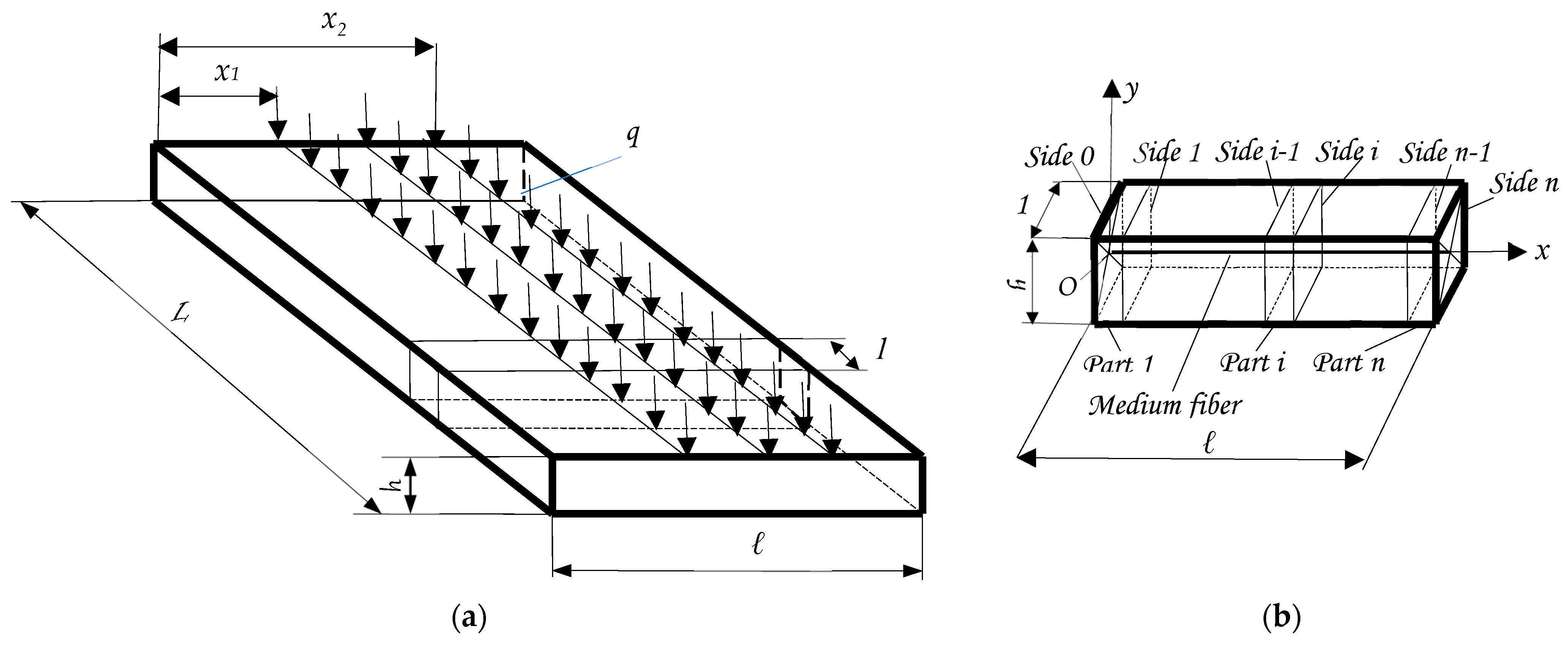
2.1. Analytical Approach for a Long Rectangular Plate

For a long rectangular plate, a uniform vertical load is considered, acting over a surface area [(x₂ − x₁) × L], with a load density q(x) as shown in Figure 1a.

It is considered that the plate is subjected to a force F, illustrated in Figure 2b [4].

The bending moment resulting from a single external load is denoted by m(x). The load density q(x) is defined per unit length. Expression (1) [4] gives the total moment M(x):

$$M\left(x\right)=m\left(x\right)+Ff\left(x\right),$$

(1)

When f(x) represents the arrow corresponding to section x, the bending moment m(x) can be expressed as shown in Equation (2) [4]:

$${\displaystyle \frac{d^{2}m\left(x\right)}{d{x}^2}}=q\left(x\right),$$

(2)

For the average deformed fiber, the differential equation can be written as (3) [4]:

$${\displaystyle \frac{d^{4}m\left(x\right)}{d{x}^4}}-{\displaystyle \frac{12\left(1-{\nu }^2\right)}{E{h}^3}}·{\displaystyle \frac{d^{2}f\left(x\right)}{d{x}^2}}F={\displaystyle \frac{12\left(1-{\nu }^2\right)}{E{h}^3}}q\left(x\right),$$

(3)

where R denotes the bending stiffness of a plate with thickness h as (4) [4]:

$$R={\displaystyle \frac{E{h}^3}{12\left(1-{\nu }^2\right)}},$$

(4)

When E is the Young’s modulus, h is the thickness of the plate, ν is the Poisson’s coefficient, expression (4) becomes (5) [4]:

$${\displaystyle \frac{d^{4}m\left(x\right)}{d{x}^4}}-{\displaystyle \frac{1}{R}}{\displaystyle \frac{d^{2}f\left(x\right)}{d{x}^2}}F={\displaystyle \frac{1}{R}}q\left(x\right),$$

(5)

The following is noted by (6) [4]:

$${\beta }^2={\displaystyle \frac{1}{R}}F,$$

(6)

and the differential Equation (5) becomes as (7) [4]:

$${\displaystyle \frac{d^{4}m\left(x\right)}{d{x}^4}}-{\beta }^2{\displaystyle \frac{d^{2}f\left(x\right)}{d{x}^2}}={\displaystyle \frac{1}{R}}q\left(x\right),$$

(7)

The solution of the differential Equation (7) without the second term is as (8):

$$f_1\left(x\right)=D_1 ch\left(\beta x\right)+D_2 sh\left(\beta x\right)+D_{3}x+D_4,$$

(8)

the particular solution is (9) [4]:

$$f^{*}\left(x\right)={\displaystyle \frac{1}{R{\beta }^3}}\underset{0}{\overset{x}{\int }}\left[sh\left(\beta \left(x-t\right)\right)-\beta \left(x-t\right)\right]q\left(t\right)dt,$$

(9)

and must verify the conditions in (10) [4]:

$$f^{*}\left(0\right)=f^{*\prime }\left(0\right)=f^{*″}\left(0\right)=f^{*‴}\left(0\right),$$

(10)

For x = 0 (11), it can be written as follows [4]:

$$\left\{\begin{array}{c}f\left(0\right)=f_0\\ \omega \left(0\right)={\omega }_0\\ M\left(0\right)=M_0 \\ T\left(0\right)=T_0\end{array}\right.,$$

(11)

The integration constants D_i, i = 1, 4 are as in (12) [4]:

$$\left\{\begin{array}{c}{f}_0=D_1+D_4\\ {\omega }_0=\beta D_2+D_3\\ M_0={\beta }^2{D}_1{D}_4\\ T_0=-{\beta }^3{D}_2{D}_4\end{array}\right.,$$

(12)

The four integration constants depending on efforts and deformations are as in (13) [4]:

$$\left\{\begin{array}{c}{D}_1={\displaystyle \frac{1}{{\beta }^{2}R}}{M}_0\\ D_2=-{\displaystyle \frac{1}{{\beta }^{3}R}}{T}_0\\ D_3={\omega }_0+{\displaystyle \frac{1}{{\beta }^{3}R}}{T}_0\\ D_4=f_0-{\displaystyle \frac{1}{{\beta }^{2}R}}{M}_0\end{array}\right.,$$

(13)

The mathematical expression of the deformation is as (14), [4]:

$$\begin{gathered} f\left(x\right)=f_0+{\omega }_{0}x+{\displaystyle \frac{ch\left(\beta x\right)-1}{{\beta }^{2}R}}{M}_0+{\displaystyle \frac{\beta x-sh\left(\beta x\right)}{{\beta }^{3}R}}{T}_0 \\ \hspace{1em}\hspace{1em}\hspace{1em}\hspace{1em}\hspace{1em}\hspace{1em}\hspace{1em}\hspace{1em} +{\displaystyle \frac{1}{{\beta }^{3}R}}\underset{0}{\overset{x}{\int }}\left[sh\left(\beta \left(x-t\right)\right)-\beta \left(x-t\right)\right]q\left(t\right)dt, \end{gathered}$$

(14)

2.2. TMM-Based Calculation Algorithm for Long Rectangular Plates

The long rectangular plate is discretized in its lengths into unit beams, as in Figure 1a,b [4]. The beam, with a unit width, is discretized into parts perpendicular to the Ox axis. Each part possesses a left and a right side, with a state vector assigned to each side.

Each segment of the unit-width beam has an associated transfer matrix, as shown in Figure 2a, and undergoes deformation as illustrated in Figure 2b [4]. The first part, located on the left of the beam, has its left side labeled 0 and its right side labeled 1. The final part, on the right side of the beam, the last side n, is labeled n, resulting in a total of n parts and n + 1 sides [4]. A state vector is associated with each side. This state vector consists of four components: the arrow f, the rotation ω, the bending moment M, and the shear force T. For a given side x, the state vector can be written as in Equation (15) [4], with the state vector and each of its components consistently indexed according to the side they are associated with:

$$\left\{U\left(x\right)\right\}={{\left\{U\right\}}_x=\left\{f\left(x\right), \omega \left(x\right), M\left(x\right),T\left(x\right)\right\}}^{-1}={\left\{f_x,{\omega }_x,M_x,T_x\right\}}^{-1},$$

(15)

For the side 0, for x = 0, it can be written as in (16) [4]:

$$\left\{U\left(0\right)\right\}={{\left\{U\right\}}_0=\left\{f\left(0\right), \omega \left(0\right), M\left(0\right),T\left(0\right)\right\}}^{-1}={\left\{f_0,{\omega }_0,M_0,T_0\right\}}^{-1},$$

(16)

For the last part n, at the right end of the beam—corresponding to the final side n, where x = l—the state vector is given by (17) [4]:

$$\left\{U\left(l\right)\right\}={{\left\{U\right\}}_l=\left\{f\left(l\right), \omega \left(l\right), M\left(l\right),T\left(l\right)\right\}}^{-1}={\left\{f_l,{\omega }_l,M_l,T_l\right\}}^{-1},$$

(17)

A transfer matrix [TM]_x is associated with each part x of the beam, linking the two consecutive sides of that part. For part 1, this relationship is defined by the matrix Equation (18) [4]:

$${{\left\{U\right\}}_1=\left[TM\right]}_1{\left\{U\right\}}_0+{\left\{U_e\right\}}_1,$$

(18)

where {Ue}₁ is the state vector corresponding to the external forces on part 1 [4]. The matrix relation for a given part x can be written as in (19) [4]:

$${{\left\{U\right\}}_x=\left[TM\right]}_x{\left\{U\right\}}_0+{\left\{U_e\right\}}_x,$$

(19)

At the end of the unit beam, where x = l, Equation (19) becomes Equation (20) [4]:

$${{\left\{U\right\}}_l=\left[TM\right]}_l{\left\{U\right\}}_0+{\left\{U_e\right\}}_l,$$

(20)

In matrix relation (20), the state vector at the origin is determined based on the end conditions. Once this is known, the remaining unknown components at face n, on the right end of the beam, can be computed. Returning to the matrix relation (19), by assigning different values to xxx, all the state vectors for a unit beam can be calculated. By extrapolation, this process allows the calculation of all the state vectors for the entire long rectangular plate.

3. Applications of the TMM for the Calculation of Long Rectangular Plates Under Uniform Loads Acting on Different Surfaces

For the unit beam embedded at both ends and subjected to uniform loads, the following loading cases will be presented:

• A uniform vertical load q, acting over a length (x₂ − x₁) of the unit beam, as shown in Figure 3;
• A uniform vertical load q, acting from section x₁ to the right end of the unit beam, over a length of (l − x₁), as shown in Figure 4;
• A uniform vertical load q, acting along the length x₁, as shown in Figure 5;
• A uniform vertical load q, acting along the entire length l of the unit beam, as shown in Figure 6;
• Two uniform vertical loads: q₁ acts over a length (x₂ − x₁) of the unit beam, and q₂ acts over a length (x₄ − x₃) of the same unit beam, as shown in Figure 7a; and two uniform vertical loads: q₁ acts over a length (x₂ − x₁), and q₂ over (x₄ − x₃), as shown in Figure 7b.

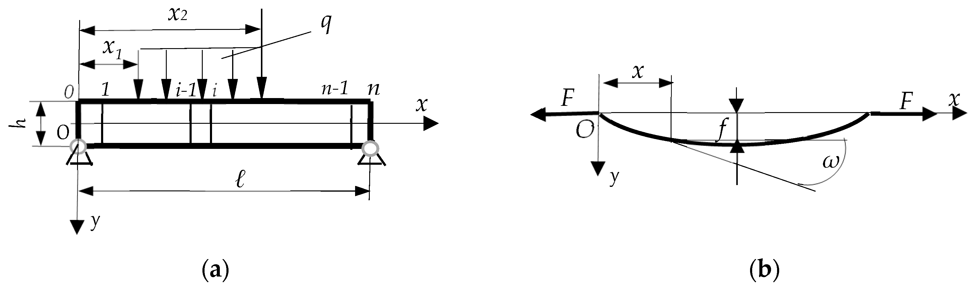
3.1. Unit Beam Embedded at Both Ends, Subjected to a Uniform Vertical Load q Acting over a Length (x₂ − x₁) of the Beam, as Shown in Figure 3

To begin, the unit beam was considered, embedded at the two edges, charged with a uniform distributed load along the length (x₂ – x₁), as in Figure 3.

The charge density, in this case, can be written as (21):

$$q\left(x\right)=-q\left[Y\left(x-x_1\right)-Y\left(x-x_2\right)\right]$$

(21)

Y being Heaviside’s function. With Dirac’s and Heaviside’s functions and operators, the state vector {U_e}_x corresponding at exterior load is as (22):

$${\left\{U_e\right\}}_x=\left\{\begin{array}{c}-{\displaystyle \frac{1}{{\beta }^{3}R}}q\left[Y\left(x-x_1\right){\displaystyle \frac{ch\left(\beta \left(x-x_1\right)\right)-1}{\beta }}-{\displaystyle \frac{\beta }{2}}{\left(x-x_1\right)}^2-Y\left(x-x_2\right){\displaystyle \frac{ch \left(\beta \left(x-x_2\right)\right)-1}{\beta }}+{\displaystyle \frac{\beta }{2}}{\left(x-x_2\right)}^2\right]\\ -{\displaystyle \frac{1}{{\beta }^{2}R}}q\left[Y\left(x-x_1\right)sh\left(\beta \left(x-x_1\right)\right)-\beta \left(x-x_1\right)-Y\left(x-x_2\right)sh \left(\beta \left(x-x_2\right)\right)+\beta \left(x-x_2\right)\right]\\ -{\displaystyle \frac{1}{{\beta }^2}}q\left[Y\left(x-x_1\right)ch\left(\beta \left(x-x_1\right)\right)-Y\left(x-x_2\right)ch\left(\beta \left(x-x_2\right)\right)\right]\\ {\displaystyle \frac{1}{\beta }}q\left[Y\left(x-x_1\right) sh \left(\beta \left(x-x_1\right)\right)-Y\left(x-x_2\right) sh\left(\beta \left(x-x_2\right)\right)\right]\end{array}\right\},$$

(22)

The matrix relation is as in (23):

$$\begin{gathered} \left\{\begin{array}{c}f\left(x\right)\\ \omega \left(x\right)\\ M\left(x\right)\\ T\left(x\right)\end{array}\right\}=\left[\begin{array}{cccc}1& x& {\displaystyle \frac{ch\left(\beta x\right)-1}{{\beta }^{2}R}}& {\displaystyle \frac{\beta x-sh\left(\beta x\right)}{{\beta }^{3}R}}\\ 0& 1& {\displaystyle \frac{sh\left(\beta x\right)}{\beta R}}& -{\displaystyle \frac{ch\left(\beta x\right)-1}{{\beta }^{2}R}}\\ 0& 0& ch\left(\beta x\right)& -{\displaystyle \frac{sh\left(\beta x\right)}{\beta }}\\ 0& 0& -\beta sh\left(\beta x\right)& ch\left(\beta x\right)\end{array}\right]\left\{\begin{array}{c}{f}_0\\ {\omega }_0\\ M_0\\ T_0\end{array}\right\}+ \\ +\left\{\begin{array}{c}-{\displaystyle \frac{1}{{\beta }^{3}R}}q\left[Y\left(x-x_1\right){\displaystyle \frac{ch\left(\beta \left(x-x_1\right)\right)-1}{\beta }}-{\displaystyle \frac{\beta }{2}}{\left(x-x_1\right)}^2-Y\left(x-x_2\right){\displaystyle \frac{ch \left(\beta \left(x-x_2\right)\right)-1}{\beta }}+{\displaystyle \frac{\beta }{2}}{\left(x-x_2\right)}^2\right]\\ -{\displaystyle \frac{1}{{\beta }^{2}R}}q\left[Y\left(x-x_1\right)sh\left(\beta \left(x-x_1\right)\right)-\beta \left(x-x_1\right)-Y\left(x-x_2\right)sh\left(\beta \left(x-x_2\right)\right)+\beta \left(x-x_2\right)\right]\\ -{\displaystyle \frac{1}{{\beta }^2}}q\left[Y\left(x-x_1\right)ch\left(\beta \left(x-x_1\right)\right)-Y\left(x-x_2\right)ch\left(\beta \left(x-x_2\right)\right)\right]\\ {\displaystyle \frac{1}{\beta }}q\left[Y\left(x-x_1\right) sh\left(\beta \left(x-x_1\right)\right)-Y\left(x-x_2\right) sh\left(\beta \left(x-x_2\right)\right)\right]\end{array}\right\}, \end{gathered}$$

(23)

or, with Dirac’s and Heaviside’s functions and operators, (23) becomes (24):

$$\begin{gathered} \left\{\begin{array}{c}f\left(x\right)\\ \omega \left(x\right)\\ M\left(x\right)\\ T\left(x\right)\end{array}\right\}=\left[\begin{array}{cccc}1& x& {\displaystyle \frac{ch\left(\beta x\right)-1}{{\beta }^{2}R}}& {\displaystyle \frac{\beta x-sh\left(\beta x\right)}{{\beta }^{3}R}}\\ 0& 1& {\displaystyle \frac{sh\left(\beta x\right)}{\beta R}}& -{\displaystyle \frac{ch\left(\beta x\right)-1}{{\beta }^{2}R}}\\ 0& 0& ch\left(\beta x\right)& -{\displaystyle \frac{sh\left(\beta x\right)}{\beta }}\\ 0& 0& -\beta sh\left(\beta x\right)& ch\left(\beta x\right)\end{array}\right]\left\{\begin{array}{c}{f}_0\\ {\omega }_0\\ M_0\\ T_0\end{array}\right\}+ \\ \hspace{1em}\hspace{1em}\hspace{1em}\hspace{1em}\hspace{1em}\hspace{1em}+\left\{\begin{array}{c}-{\displaystyle \frac{1}{{\beta }^{3}R}}q\left[{\displaystyle \frac{ch\left(\beta \left(x-x_1\right)\right)-1}{\beta }}-{\displaystyle \frac{\beta }{2}}{\left(x-x_1\right)}^2-{\displaystyle \frac{ch\left(\beta \left(x-x_2\right)\right)-1}{\beta }}+{\displaystyle \frac{\beta }{2}}{\left(x-x_2\right)}^2\right]\\ -{\displaystyle \frac{1}{{\beta }^{2}R}}q\left[sh\left(\beta \left(x-x_1\right)\right)-\beta \left(x-x_1\right)-sh\left(\beta \left(x-x_2\right)\right)+\beta \left(x-x_2\right)\right]\\ -{\displaystyle \frac{1}{{\beta }^2}}q\left[ch\left(\beta \left(x-x_1\right)\right)-ch\left(\beta \left(x-x_2\right)\right)\right]\\ {\displaystyle \frac{1}{\beta }}q\left[ sh\left(\beta \left(x-x_1\right)\right)-sh\left(\beta \left(x-x_2\right)\right)\right]\end{array}\right\}, \end{gathered}$$

(24)

For x = l, (25) is obtained:

$$\begin{gathered} \left\{\begin{array}{c}f\left(l\right)\\ \omega \left(l\right)\\ M\left(l\right)\\ T\left(l\right)\end{array}\right\}=\left[\begin{array}{cccc}1& l& {\displaystyle \frac{ch\left(\beta l\right)-1}{{\beta }^{2}R}}& {\displaystyle \frac{\beta l-sh\left(\beta l\right)}{{\beta }^{3}R}}\\ 0& 1& {\displaystyle \frac{sh\left(\beta l\right)}{\beta R}}& -{\displaystyle \frac{ch\left(\beta l\right)-1}{{\beta }^{2}R}}\\ 0& 0& ch\left(\beta l\right)& -{\displaystyle \frac{sh\left(\beta l\right)}{\beta }}\\ 0& 0& -\beta sh\left(\beta l\right)& ch\left(\beta l\right)\end{array}\right]\left\{\begin{array}{c}{f}_0\\ {\omega }_0\\ M_0\\ T_0\end{array}\right\}+ \\ \hspace{1em}\hspace{1em}\hspace{1em}\hspace{1em}\hspace{1em}\hspace{1em}+\left\{\begin{array}{c}-{\displaystyle \frac{1}{{\beta }^{3}R}}q\left[{\displaystyle \frac{ch\left(\beta \left(l-x_1\right)\right)-1}{\beta }}-{\displaystyle \frac{\beta }{2}}{\left(l-x_1\right)}^2-{\displaystyle \frac{ch\left(\beta \left(l-x_2\right)\right)-1}{\beta }}+{\displaystyle \frac{\beta }{2}}{\left(l-x_2\right)}^2\right]\\ -{\displaystyle \frac{1}{{\beta }^{2}R}}q\left[sh\left(\beta \left(l-x_1\right)\right)-\beta \left(l-x_1\right)-sh\left(\beta \left(l-x_2\right)\right)+\beta \left(l-x_2\right)\right]\\ -{\displaystyle \frac{1}{{\beta }^2}}q\left[ch\left(\beta \left(l-x_1\right)\right)-ch\left(\beta \left(l-x_2\right)\right)\right]\\ {\displaystyle \frac{1}{\beta }}q\left[sh\left(\beta \left(l-x_1\right)\right)-sh\left(\beta \left(l-x_2\right)\right)\right]\end{array}\right\}, \end{gathered}$$

(25)

The conditions for the two embedded ends of the beam are as in (26):

$$\left\{\begin{array}{c}{f}_0=0\\ {\omega }_0=0\\ f\left(l\right)=0 \\ \omega \left(l\right)=0\end{array}\right.,$$

(26)

With (26), the matrix relation (25) becomes (27):

$$\begin{gathered} \left\{\begin{array}{c}0\\ 0\\ M\left(l\right)\\ T\left(l\right)\end{array}\right\}=\left[\begin{array}{cccc}1& l& {\displaystyle \frac{ch\left(\beta l\right)-1}{{\beta }^{2}R}}& {\displaystyle \frac{\beta l-sh\left(\beta l\right)}{{\beta }^{3}R}}\\ 0& 1& {\displaystyle \frac{sh\left(\beta l\right)}{\beta R}}& -{\displaystyle \frac{ch\left(\beta l\right)-1}{{\beta }^{2}R}}\\ 0& 0& ch\left(\beta l\right)& -{\displaystyle \frac{sh\left(\beta l\right)}{\beta }}\\ 0& 0& -\beta sh\left(\beta l\right)& ch\left(\beta l\right)\end{array}\right]\left\{\begin{array}{c}0\\ 0\\ M_0\\ T_0\end{array}\right\}+ \\ \hspace{1em}\hspace{1em}\hspace{1em}\hspace{1em}\hspace{1em}\hspace{1em}+\left\{\begin{array}{c}-{\displaystyle \frac{1}{{\beta }^{3}R}}q\left[{\displaystyle \frac{ch\left(\beta \left(l-x_1\right)\right)-1}{\beta }}-{\displaystyle \frac{\beta }{2}}{\left(l-x_1\right)}^2-{\displaystyle \frac{ch\left(\beta \left(l-x_2\right)\right)-1}{\beta }}+{\displaystyle \frac{\beta }{2}}{\left(l-x_2\right)}^2\right]\\ -{\displaystyle \frac{1}{{\beta }^{2}R}}q\left[sh\left(\beta \left(l-x_1\right)\right)-\beta \left(l-x_1\right)-sh\left(\beta \left(l-x_2\right)\right)+\beta \left(l-x_2\right)\right]\\ -{\displaystyle \frac{1}{{\beta }^2}}q\left[ch\left(\beta \left(l-x_1\right)\right)-ch\left(\beta \left(l-x_2\right)\right)\right]\\ {\displaystyle \frac{1}{\beta }}q\left[sh\left(\beta \left(l-x_1\right)\right)-sh\left(\beta \left(l-x_2\right)\right)\right]\end{array}\right\}, \end{gathered}$$

(27)

3.2. Unit Beam Embedded at the Two Edges Charged with Uniform Load q Which Acts from Section x₁ to the Right End of the Beam, Along a Length (l − x₁), as in Figure 4

The unit beam was considered, embedded at the two edges, charged with a uniform distributed load along the length (l − x₁), as in Figure 4.

The charge density can be written as (28):

$$q\left(x\right)=-qY\left(x-x_1\right),$$

(28)

Y being Heaviside’s function. The vector of exterior loads corresponding to section x is as in (29):

$${\left\{U_e\right\}}_x=\left\{\begin{array}{c}-{\displaystyle \frac{1}{{\beta }^{3}R}}qY\left(x-x_1\right)\left[{\displaystyle \frac{ch\left(\beta \left(x-x_1\right)\right)-1}{\beta }}-{\displaystyle \frac{\beta }{2}}{\left(x-x_1\right)}^2\right]\\ -{\displaystyle \frac{1}{{\beta }^{2}R}}qY\left(x-x_1\right)\left[sh\left(\beta \left(x-x_1\right)\right)-\beta \left(x-x_1\right)\right]\\ -{\displaystyle \frac{1}{{\beta }^2}}qY\left(x-x_1\right)\left[ch\left(\beta \left(x-x_1\right)\right)-1\right]\\ {\displaystyle \frac{1}{\beta }}qY\left(x-x_1\right) sh\left(\beta \left(x-x_1\right)\right)\end{array}\right\},$$

(29)

The matrix relation is as in (30):

$$\left\{\begin{array}{c}f\left(x\right)\\ \omega \left(x\right)\\ M\left(x\right)\\ T\left(x\right)\end{array}\right\}=\left[\begin{array}{cccc}1& x& {\displaystyle \frac{ch\left(\beta x\right)-1}{{\beta }^{2}R}}& {\displaystyle \frac{\beta x-sh\left(\beta x\right)}{{\beta }^{3}R}}\\ 0& 1& {\displaystyle \frac{sh\left(\beta x\right)}{\beta R}}& -{\displaystyle \frac{ch\left(\beta x\right)-1}{{\beta }^{2}R}}\\ 0& 0& ch\left(\beta x\right)& -{\displaystyle \frac{sh\left(\beta x\right)}{\beta }}\\ 0& 0& -\beta sh\left(\beta x\right)& ch\left(\beta x\right)\end{array}\right]\left\{\begin{array}{c}{f}_0\\ {\omega }_0\\ M_0\\ T_0\end{array}\right\}+\left\{\begin{array}{c}-{\displaystyle \frac{1}{{\beta }^{3}R}}qY\left(x-x_1\right)\left[{\displaystyle \frac{ch\left(\beta \left(x-x_1\right)\right)-1}{\beta }}-{\displaystyle \frac{\beta }{2}}{\left(x-x_1\right)}^2\right]\\ -{\displaystyle \frac{1}{{\beta }^{2}R}}qY\left(x-x_1\right)\left[sh\left(\beta \left(x-x_1\right)\right)-\beta \left(x-x_1\right)\right]\\ -{\displaystyle \frac{1}{{\beta }^2}}qY\left(x-x_1\right)\left[ch\left(\beta \left(x-x_1\right)\right)-1\right]\\ {\displaystyle \frac{1}{\beta }}qY\left(x-x_1\right) sh\left(\beta \left(x-x_1\right)\right)\end{array}\right\}$$

(30)

or, with Dirac’s and Heaviside’s functions and operators, (30) becomes (31):

$$\left\{\begin{array}{c}f\left(x\right)\\ \omega \left(x\right)\\ M\left(x\right)\\ T\left(x\right)\end{array}\right\}=\left[\begin{array}{cccc}1& x& {\displaystyle \frac{ch\left(\beta x\right)-1}{{\beta }^{2}R}}& {\displaystyle \frac{\beta x-sh\left(\beta x\right)}{{\beta }^{3}R}}\\ 0& 1& {\displaystyle \frac{sh\left(\beta x\right)}{\beta R}}& -{\displaystyle \frac{ch\left(\beta x\right)-1}{{\beta }^{2}R}}\\ 0& 0& ch\left(\beta x\right)& -{\displaystyle \frac{sh\left(\beta x\right)}{\beta }}\\ 0& 0& -\beta sh\left(\beta x\right)& ch\left(\beta x\right)\end{array}\right]\left\{\begin{array}{c}{f}_0\\ {\omega }_0\\ M_0\\ T_0\end{array}\right\}+\left\{\begin{array}{c}-{\displaystyle \frac{1}{{\beta }^{3}R}}q\left[{\displaystyle \frac{ch\left(\beta \left(x-x_1\right)\right)-1}{\beta }}-{\displaystyle \frac{\beta }{2}}{\left(x-x_1\right)}^2\right]\\ -{\displaystyle \frac{1}{{\beta }^{3}R}}q\left[sh\left(\beta \left(x-x_1\right)\right)-\beta \left(x-x_1\right)\right]\\ -{\displaystyle \frac{1}{{\beta }^2}}q\left[ch\left(\beta \left(x-x_1\right)\right)-1\right]\\ {\displaystyle \frac{1}{\beta }}q sh\left(\beta \left(x-x_1\right)\right)\end{array}\right\}$$

(31)

For x = l, (32) can be obtained:

$$\left\{\begin{array}{c}f\left(l\right)\\ \omega \left(l\right)\\ M\left(l\right)\\ T\left(l\right)\end{array}\right\}=\left[\begin{array}{cccc}1& l& {\displaystyle \frac{ch\left(\beta l\right)-1}{{\beta }^{2}R}}& {\displaystyle \frac{\beta l-sh\left(\beta l\right)}{{\beta }^{3}R}}\\ 0& 1& {\displaystyle \frac{sh\left(\beta l\right)}{\beta R}}& -{\displaystyle \frac{ch\left(\beta l\right)-1}{{\beta }^{2}R}}\\ 0& 0& ch\left(\beta l\right)& -{\displaystyle \frac{sh\left(\beta l\right)}{\beta }}\\ 0& 0& -\beta sh\left(\beta l\right)& ch\left(\beta l\right)\end{array}\right]\left\{\begin{array}{c}{f}_0\\ {\omega }_0\\ M_0\\ T_0\end{array}\right\}+\left\{\begin{array}{c}-{\displaystyle \frac{1}{{\beta }^{3}R}}q\left[{\displaystyle \frac{ch\left(\beta \left(l-x_1\right)\right)-1}{\beta }}-{\displaystyle \frac{\beta }{2}}{\left(l-x_1\right)}^2\right]\\ -{\displaystyle \frac{1}{{\beta }^{3}R}}q\left[sh\left(\beta \left(l-x_1\right)\right)-\beta \left(l-x_1\right)\right]\\ -{\displaystyle \frac{1}{{\beta }^2}}q\left[ch\left(\beta \left(l-x_1\right)\right)-1\right]\\ {\displaystyle \frac{1}{\beta }}q sh\left(\beta \left(l-x_1\right)\right)\end{array}\right\}$$

(32)

The conditions for the two embedded ends of the beam are as in (26):

$$\left\{\begin{array}{c}{f}_0=0\\ {\omega }_0=0\\ f\left(l\right)=0 \\ \omega \left(l\right)=0\end{array}\right.,$$

With (26), the matrix relation (32) becomes (33):

$$\left\{\begin{array}{c}0\\ 0\\ M\left(l\right)\\ T\left(l\right)\end{array}\right\}=\left[\begin{array}{cccc}1& l& {\displaystyle \frac{ch\left(\beta l\right)-1}{{\beta }^{2}R}}& {\displaystyle \frac{\beta l-sh\left(\beta l\right)}{{\beta }^{3}R}}\\ 0& 1& {\displaystyle \frac{sh\left(\beta l\right)}{\beta R}}& -{\displaystyle \frac{ch\left(\beta l\right)-1}{{\beta }^{2}R}}\\ 0& 0& ch\left(\beta l\right)& -{\displaystyle \frac{sh\left(\beta l\right)}{\beta }}\\ 0& 0& -\beta sh\left(\beta l\right)& ch\left(\beta l\right)\end{array}\right]\left\{\begin{array}{c}0\\ 0\\ M_0\\ T_0\end{array}\right\}+\left\{\begin{array}{c}-{\displaystyle \frac{1}{{\beta }^{3}R}}q\left[{\displaystyle \frac{ch\left(\beta \left(l-x_1\right)\right)-1}{\beta }}-{\displaystyle \frac{\beta }{2}}{\left(l-x_1\right)}^2\right]\\ -{\displaystyle \frac{1}{{\beta }^{3}R}}q \left[sh\left(\beta \left(l-x_1\right)\right)-\beta \left(l-x_1\right)\right]\\ -{\displaystyle \frac{1}{{\beta }^2}}q \left[ch\left(\beta \left(l-x_1\right)\right)-1\right]\\ {\displaystyle \frac{1}{\beta }}q sh\left(\beta \left(l-x_1\right)\right)\end{array}\right\}$$

(33)

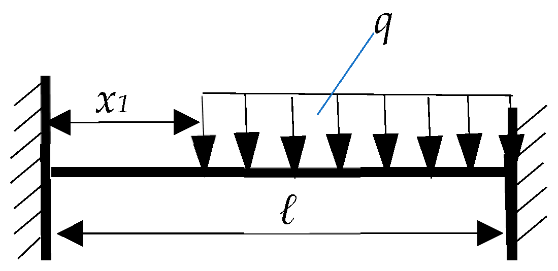
3.3. Unit Beam Embedded at the Two Edges Charged with Uniform Load q Which Acts Along the Length x₁, as in Figure 5

This case can be treated in the same way as the case presented in Section 3.1, putting the following conditions (34):

$$\left\{\begin{array}{c}{x}_1=0\\ x_2=x_1\end{array}\right.$$

(34)

The charge density, in this case, can be written as in (35):

$$q\left(x\right)=-q\left[Y\left(x\right)-Y\left(x-x_1\right)\right]$$

(35)

Y being Heaviside’s function. With Dirac’s and Heaviside’s functions and operators, the state vector {U_e}_x corresponding at an exterior load is as in (36):

$${\left\{U_e\right\}}_x=\left\{\begin{array}{c}-{\displaystyle \frac{1}{{\beta }^{3}R}}q\left[Y\left(x\right){\displaystyle \frac{ch\left(\beta x\right)-1}{\beta }}-{\displaystyle \frac{\beta }{2}}{x}^2-Y\left(x-x_1\right){\displaystyle \frac{ch\left(\beta \left(x-x_1\right)\right)-1}{\beta }}+{\displaystyle \frac{\beta }{2}}{\left(x-x_1\right)}^2\right]\\ -{\displaystyle \frac{1}{{\beta }^{2}R}}q\left[Y\left(x\right)sh\left(\beta x\right)-\beta x-Y\left(x-x_1\right)sh\left(\beta \left(x-x_1\right)\right)+\beta \left(x-x_1\right)\right]\\ -{\displaystyle \frac{1}{{\beta }^2}}q\left[Y\left(x\right)ch\left(\beta x\right)-Y\left(x-x_1\right)ch\left(\beta \left(x-x_1\right)\right)\right]\\ {\displaystyle \frac{1}{\beta }}q\left[Y\left(x\right)sh\left(\beta x\right)-Y\left(x-x_1\right)sh\left(\beta \left(x-x_1\right)\right)\right]\end{array}\right\},$$

(36)

The matrix relation is as in (37):

$$\begin{gathered} \left\{\begin{array}{c}f\left(x\right)\\ \omega \left(x\right)\\ M\left(x\right)\\ T\left(x\right)\end{array}\right\}=\left[\begin{array}{cccc}1& x& {\displaystyle \frac{ch\left(\beta x\right)-1}{{\beta }^{2}R}}& {\displaystyle \frac{\beta x-sh\left(\beta x\right)}{{\beta }^{3}R}}\\ 0& 1& {\displaystyle \frac{sh\left(\beta x\right)}{\beta R}}& -{\displaystyle \frac{ch\left(\beta x\right)-1}{{\beta }^{2}R}}\\ 0& 0& ch\left(\beta x\right)& -{\displaystyle \frac{sh\left(\beta x\right)}{\beta }}\\ 0& 0& -\beta sh\left(\beta x\right)& ch\left(\beta x\right)\end{array}\right]\left\{\begin{array}{c}{f}_0\\ {\omega }_0\\ M_0\\ T_0\end{array}\right\}+ \\ \hspace{1em}\hspace{1em}\hspace{1em}\hspace{1em}\hspace{1em}\hspace{1em}+\left\{\begin{array}{c}-{\displaystyle \frac{1}{{\beta }^{3}R}}q\left[Y\left(x\right){\displaystyle \frac{ch\left(\beta x\right)-1}{\beta }}-{\displaystyle \frac{\beta }{2}}{x}^2-Y\left(x-x_1\right){\displaystyle \frac{ch\left(\beta \left(x-x_1\right)\right)-1}{\beta }}+{\displaystyle \frac{\beta }{2}}{\left(x-x_1\right)}^2\right]\\ -{\displaystyle \frac{1}{{\beta }^{2}R}}q\left[Y\left(x\right)sh\left(\beta x\right)-\beta x-Y\left(x-x_1\right)sh\left(\beta \left(x-x_1\right)\right)+\beta \left(x-x_1\right)\right]\\ -{\displaystyle \frac{1}{{\beta }^2}}q\left[Y\left(x\right)ch\left(\beta x\right)-Y\left(x-x_1\right)ch\left(\beta \left(x-x_1\right)\right)\right]\\ {\displaystyle \frac{1}{\beta }}q\left[Y\left(x\right)sh\left(\beta x\right)-Y\left(x-x_1\right)sh\left(\beta \left(x-x_1\right)\right)\right]\end{array}\right\}, \end{gathered}$$

(37)

With Dirac’s and Heaviside’s functions and operators, the matrix relation (37) becomes (38):

$$\begin{gathered} \left\{\begin{array}{c}f\left(x\right)\\ \omega \left(x\right)\\ M\left(x\right)\\ T\left(x\right)\end{array}\right\}=\left[\begin{array}{cccc}1& x& {\displaystyle \frac{ch\left(\beta x\right)-1}{{\beta }^{2}R}}& {\displaystyle \frac{\beta x-sh\left(\beta x\right)}{{\beta }^{3}R}}\\ 0& 1& {\displaystyle \frac{sh\left(\beta x\right)}{\beta R}}& -{\displaystyle \frac{ch\left(\beta x\right)-1}{{\beta }^{2}R}}\\ 0& 0& ch\left(\beta x\right)& -{\displaystyle \frac{sh \left(\beta x\right)}{\beta }}\\ 0& 0& -\beta sh\left(\beta x\right)& ch\left(\beta x\right)\end{array}\right]\left\{\begin{array}{c}{f}_0\\ {\omega }_0\\ M_0\\ T_0\end{array}\right\}+ \\ \hspace{1em}\hspace{1em}\hspace{1em}\hspace{1em}\hspace{1em}\hspace{1em}+\left\{\begin{array}{c}-{\displaystyle \frac{1}{{\beta }^{3}R}}q\left[{\displaystyle \frac{ch\left(\beta x\right)-1}{\beta }}-{\displaystyle \frac{\beta }{2}}{x}^2-{\displaystyle \frac{ch\left(\beta \left(x-x_1\right)\right)-1}{\beta }}+{\displaystyle \frac{\beta }{2}}{\left(x-x_1\right)}^2\right]\\ -{\displaystyle \frac{1}{{\beta }^{2}R}}q\left[sh\left(\beta x\right)-\beta x-sh\left(\beta \left(x-x_1\right)\right)+\beta \left(x-x_1\right)\right]\\ -{\displaystyle \frac{1}{{\beta }^2}}q \left[ch\left(\beta x\right)-ch\left(\beta \left(x-x_1\right)\right)\right]\\ {\displaystyle \frac{1}{\beta }}q \left[sh\left(\beta x\right)-sh\left(\beta \left(x-x_1\right)\right)\right]\end{array}\right\}, \end{gathered}$$

(38)

For x = l, (39) is obtained:

$$\begin{gathered} \left\{\begin{array}{c}f\left(l\right)\\ \omega \left(l\right)\\ M\left(l\right)\\ T\left(l\right)\end{array}\right\}=\left[\begin{array}{cccc}1& l& {\displaystyle \frac{ch\left(\beta l\right)-1}{{\beta }^{2}R}}& {\displaystyle \frac{\beta l-sh\left(\beta l\right)}{{\beta }^{3}R}}\\ 0& 1& {\displaystyle \frac{sh\left(\beta l\right)}{\beta R}}& -{\displaystyle \frac{ch\left(\beta l\right)-1}{{\beta }^{2}R}}\\ 0& 0& ch\left(\beta l\right)& -{\displaystyle \frac{sh\left(\beta l\right)}{\beta }}\\ 0& 0& -\beta sh\left(\beta l\right)& ch\left(\beta l\right)\end{array}\right]\left\{\begin{array}{c}{f}_0\\ {\omega }_0\\ M_0\\ T_0\end{array}\right\}+ \\ \hspace{1em}\hspace{1em}\hspace{1em}\hspace{1em}\hspace{1em}\hspace{1em}+\left\{\begin{array}{c}-{\displaystyle \frac{1}{{\beta }^{3}R}}q\left[{\displaystyle \frac{ch\left(\beta l\right)-1}{\beta }}-{\displaystyle \frac{\beta }{2}}{l}^2-{\displaystyle \frac{ch\left(\beta \left(l-x_1\right)\right)-1}{\beta }}+{\displaystyle \frac{\beta }{2}}{\left(l-x_1\right)}^2\right]\\ -{\displaystyle \frac{1}{{\beta }^{2}R}}q \left[sh\left(\beta l\right)-\beta l-sh\left(\beta \left(l-x_1\right)\right)+\beta \left(l-x_1\right)\right]\\ -{\displaystyle \frac{1}{{\beta }^2}}q \left[ch\left(\beta l\right)-ch\left(\beta \left(l-x_1\right)\right)\right]\\ {\displaystyle \frac{1}{\beta }}q \left[sh\left(\beta l\right)-sh\left(\beta \left(l-x_1\right)\right)\right]\end{array}\right\}, \end{gathered}$$

(39)

The conditions for the two embedded ends of the beam are as in (26):

$$\left\{\begin{array}{c}{f}_0=0\\ {\omega }_0=0\\ f\left(l\right)=0 \\ \omega \left(l\right)=0\end{array}\right.,$$

With (26), the matrix relation (39) becomes (40):

$$\begin{gathered} \left\{\begin{array}{c}0\\ 0\\ M\left(l\right)\\ T\left(l\right)\end{array}\right\}=\left[\begin{array}{cccc}1& l& {\displaystyle \frac{ch\left(\beta l\right)-1}{{\beta }^{2}R}}& {\displaystyle \frac{\beta l-sh\left(\beta l\right)}{{\beta }^{3}R}}\\ 0& 1& {\displaystyle \frac{sh\left(\beta l\right)}{\beta R}}& -{\displaystyle \frac{ch\left(\beta l\right)-1}{{\beta }^{2}R}}\\ 0& 0& ch\left(\beta l\right)& -{\displaystyle \frac{sh \left(\beta l\right)}{\beta }}\\ 0& 0& -\beta sh\left(\beta l\right)& ch\left(\beta l\right)\end{array}\right]\left\{\begin{array}{c}0\\ 0\\ M_0\\ T_0\end{array}\right\}+ \\ \hspace{1em}\hspace{1em}\hspace{1em}\hspace{1em}\hspace{1em}\hspace{1em}+\left\{\begin{array}{c}-{\displaystyle \frac{1}{{\beta }^{3}R}}q\left[{\displaystyle \frac{ch\left(\beta l\right)-1}{\beta }}-{\displaystyle \frac{\beta }{2}}{l}^2-{\displaystyle \frac{ch\left(\beta \left(l-x_1\right)\right)-1}{\beta }}+{\displaystyle \frac{\beta }{2}}{\left(l-x_1\right)}^2\right]\\ -{\displaystyle \frac{1}{{\beta }^{2}R}}q \left[sh\left(\beta l\right)-\beta l-sh\left(\beta \left(l-x_1\right)\right)+\beta \left(l-x_1\right)\right]\\ -{\displaystyle \frac{1}{{\beta }^2}}q \left[ch\left(\beta l\right)-ch\left(\beta \left(l-x_1\right)\right)\right]\\ {\displaystyle \frac{1}{\beta }}q \left[sh\left(\beta l\right)-sh\left(\beta \left(l-x_1\right)\right)\right]\end{array}\right\}, \end{gathered}$$

(40)

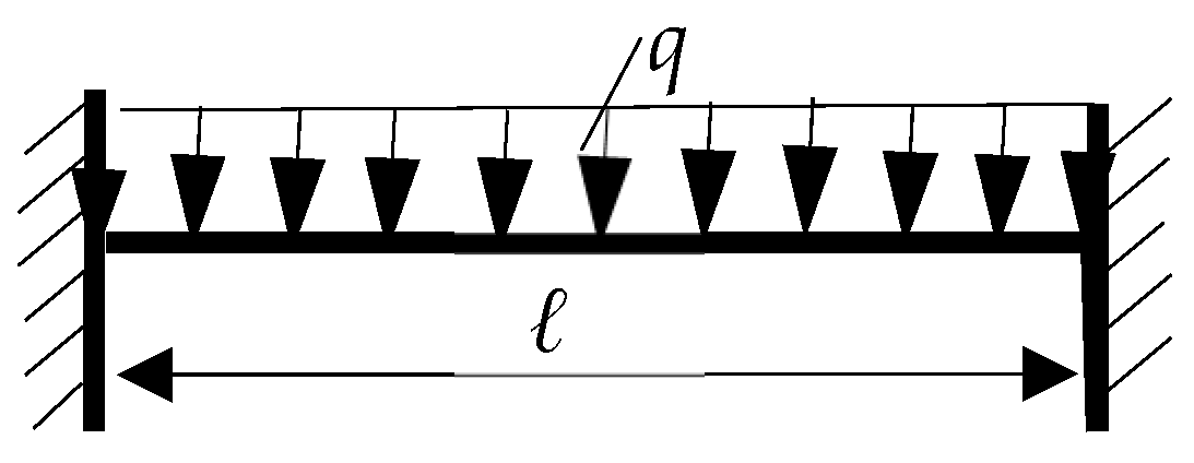
3.4. Unit Beam Embedded at the Two Edges Charged with Uniform Load q Which Acts Along the Entire Length l of the Beam, as in Figure 6

The unit beam was considered, embedded at the two edges, charged with a uniformly distributed load along the entire length l of the beam, as in Figure 6.

The charge density can be written as in (41):

$$q\left(x\right)=-qY\left(x\right),$$

(41)

Y being Heaviside’s function. The vector of exterior loads corresponding to section x is as in (42):

$${\left\{U_e\right\}}_x=\left\{\begin{array}{c}-{\displaystyle \frac{1}{{\beta }^{3}R}}qY\left(x\right)\left[{\displaystyle \frac{ch\left(\beta x\right)-1}{\beta }}-{\displaystyle \frac{\beta }{2}}{x}^2\right]\\ -{\displaystyle \frac{1}{{\beta }^{2}R}}qY\left(x\right)\left[sh\left(\beta x\right)-\beta x\right]\\ -{\displaystyle \frac{1}{{\beta }^2}}qY\left(x\right)\left[ch\left(\beta x\right)-1\right]\\ {\displaystyle \frac{1}{\beta }}qY\left(x\right) sh\left(\beta x\right)\end{array}\right\},$$

(42)

The matrix relation is as in (43):

$$\left\{\begin{array}{c}f\left(x\right)\\ \omega \left(x\right)\\ M\left(x\right)\\ T\left(x\right)\end{array}\right\}=\left[\begin{array}{cccc}1& x& {\displaystyle \frac{ch\left(\beta x\right)-1}{{\beta }^{2}R}}& {\displaystyle \frac{\beta x-sh\left(\beta x\right)}{{\beta }^{3}R}}\\ 0& 1& {\displaystyle \frac{sh\left(\beta x\right)}{\beta R}}& -{\displaystyle \frac{ch\left(\beta x\right)-1}{{\beta }^{2}R}}\\ 0& 0& ch\left(\beta x\right)& -{\displaystyle \frac{sh\left(\beta x\right)}{\beta }}\\ 0& 0& -\beta sh\left(\beta x\right)& ch\left(\beta x\right)\end{array}\right]\left\{\begin{array}{c}{f}_0\\ {\omega }_0\\ M_0\\ T_0\end{array}\right\}+\left\{\begin{array}{c}-{\displaystyle \frac{1}{{\beta }^{3}R}}qY\left(x\right)\left[{\displaystyle \frac{ch\left(\beta x\right)-1}{\beta }}-{\displaystyle \frac{\beta }{2}}{x}^2\right]\\ -{\displaystyle \frac{1}{{\beta }^{2}R}}qY\left(x\right)\left[sh\left(\beta x\right)-\beta x\right]\\ -{\displaystyle \frac{1}{{\beta }^2}}qY\left(x\right)\left[ch\left(\beta x\right)-1\right]\\ {\displaystyle \frac{1}{\beta }}qY\left(x\right)sh\left(\beta x\right)\end{array}\right\}$$

(43)

or, with Dirac’s and Heaviside’s functions and operators, (43) becomes (44):

$$\left\{\begin{array}{c}f\left(x\right)\\ \omega \left(x\right)\\ M\left(x\right)\\ T\left(x\right)\end{array}\right\}=\left[\begin{array}{cccc}1& x& {\displaystyle \frac{ch\left(\beta x\right)-1}{{\beta }^{2}R}}& {\displaystyle \frac{\beta x-sh\left(\beta x\right)}{{\beta }^{3}R}}\\ 0& 1& {\displaystyle \frac{sh\left(\beta x\right)}{\beta R}}& -{\displaystyle \frac{ch\left(\beta x\right)-1}{{\beta }^{2}R}}\\ 0& 0& ch\left(\beta x\right)& -{\displaystyle \frac{sh\left(\beta x\right)}{\beta }}\\ 0& 0& -\beta sh\left(\beta x\right)& ch\left(\beta x\right)\end{array}\right]\left\{\begin{array}{c}{f}_0\\ {\omega }_0\\ M_0\\ T_0\end{array}\right\}+\left\{\begin{array}{c}-{\displaystyle \frac{1}{{\beta }^{3}R}}q\left[{\displaystyle \frac{ch\left(\beta x\right)-1}{\beta }}-{\displaystyle \frac{\beta }{2}}{x}^2\right]\\ -{\displaystyle \frac{1}{{\beta }^{2}R}}q\left[sh\left(\beta x\right)-\beta x\right]\\ -{\displaystyle \frac{1}{{\beta }^2}}q \left[ch\left(\beta x\right)-1\right]\\ {\displaystyle \frac{1}{\beta }}q sh\left(\beta x\right)\end{array}\right\}$$

(44)

For x = l, (45) can be obtained:

$$\left\{\begin{array}{c}f\left(l\right)\\ \omega \left(l\right)\\ M\left(l\right)\\ T\left(l\right)\end{array}\right\}=\left[\begin{array}{cccc}1& l& {\displaystyle \frac{ch\left(\beta l\right)-1}{{\beta }^{2}R}}& {\displaystyle \frac{\beta l-sh\left(\beta l\right)}{{\beta }^{3}R}}\\ 0& 1& {\displaystyle \frac{sh\left(\beta l\right)}{\beta R}}& -{\displaystyle \frac{ch\left(\beta l\right)-1}{{\beta }^{2}R}}\\ 0& 0& ch\left(\beta l\right)& -{\displaystyle \frac{sh\left(\beta l\right)}{\beta }}\\ 0& 0& -\beta sh\left(\beta l\right)& ch\left(\beta l\right)\end{array}\right]\left\{\begin{array}{c}{f}_0\\ {\omega }_0\\ M_0\\ T_0\end{array}\right\}+\left\{\begin{array}{c}-{\displaystyle \frac{1}{{\beta }^{3}R}}q\left[{\displaystyle \frac{ch\left(\beta l\right)-1}{\beta }}-{\displaystyle \frac{\beta }{2}}{l}^2\right]\\ -{\displaystyle \frac{1}{{\beta }^{2}R}}q \left[sh\left(\beta l\right)-\beta l\right]\\ -{\displaystyle \frac{1}{{\beta }^2}}q \left[ch\left(\beta l\right)-1\right]\\ {\displaystyle \frac{1}{\beta }}q sh\left(\beta l\right)\end{array}\right\}$$

(45)

The conditions for the two embedded ends of the beam are as in (26):

$$\left\{\begin{array}{c}{f}_0=0\\ {\omega }_0=0\\ f\left(l\right)=0 \\ \omega \left(l\right)=0\end{array}\right.,$$

With (26), the matrix relation (45) becomes (46):

$$\left\{\begin{array}{c}0\\ 0\\ M\left(l\right)\\ T\left(l\right)\end{array}\right\}=\left[\begin{array}{cccc}1& l& {\displaystyle \frac{ch\left(\beta l\right)-1}{{\beta }^{2}R}}& {\displaystyle \frac{\beta l-sh\left(\beta l\right)}{{\beta }^{3}R}}\\ 0& 1& {\displaystyle \frac{sh\left(\beta l\right)}{\beta R}}& -{\displaystyle \frac{ch\left(\beta l\right)-1}{{\beta }^{2}R}}\\ 0& 0& ch\left(\beta l\right)& -{\displaystyle \frac{sh\left(\beta l\right)}{\beta }}\\ 0& 0& -\beta sh\left(\beta l\right)& ch\left(\beta l\right)\end{array}\right]\left\{\begin{array}{c}0\\ 0\\ M_0\\ T_0\end{array}\right\}+\left\{\begin{array}{c}-{\displaystyle \frac{1}{{\beta }^{3}R}}q\left[{\displaystyle \frac{ch\left(\beta l\right)-1}{\beta }}-{\displaystyle \frac{\beta }{2}}{l}^2\right]\\ -{\displaystyle \frac{1}{{\beta }^{2}R}}q\left[sh\left(\beta l\right)-\beta l\right]\\ -{\displaystyle \frac{1}{{\beta }^2}}q\left[ch\left(\beta l\right)-1\right]\\ {\displaystyle \frac{1}{\beta }}q sh\left(\beta l\right)\end{array}\right\}$$

(46)

3.5. Unit Beam Embedded at the Two Edges Charged with Uniform Load q Which Acts Along the Length x₁, as in Figure 7a,b

To begin, the unit beam was considered, embedded at the two edges, charged with a uniform distributed load q₁ along the length (x₂ − x₁), and q₂ along the length (x₄ − x₃), as in Figure 7a,b, but of different intensities.

The charge density, in this case, can be written as (47):

$$q\left(x\right)=-q_1\left[Y\left(x-x_1\right)-Y\left(x-x_2\right)\right]-q_2\left[Y\left(x-x_3\right)-Y\left(x-x_4\right)\right]$$

(47)

Y being Heaviside’s function. With Dirac’s and Heaviside’s functions and operators, the state vector {U_e}_x corresponding at exterior load is as in (48):

$${\left\{U_e\right\}}_x=\left\{\begin{array}{c}-{\displaystyle \frac{1}{{\beta }^{3}R}}{q}_1\left[Y\left(x-x_1\right){\displaystyle \frac{ch\left(\beta \left(x-x_1\right)\right)-1}{\beta }}-{\displaystyle \frac{\beta }{2}}{\left(x-x_1\right)}^2\right]-{\displaystyle \frac{1}{{\beta }^{3}R}}{q}_1\left[Y\left(x-x_2\right){\displaystyle \frac{ch\left(\beta \left(x-x_2\right)\right)-1}{\beta }}+{\displaystyle \frac{\beta }{2}}{\left(x-x_2\right)}^2\right]-\\ -{\displaystyle \frac{1}{{\beta }^{3}R}}{q}_2\left[Y\left(x-x_3\right){\displaystyle \frac{ch\left(\beta \left(x-x_3\right)\right)-1}{\beta }}-{\displaystyle \frac{\beta }{2}}{\left(x-x_3\right)}^2\right]-{\displaystyle \frac{1}{{\beta }^{3}R}}{q}_2\left[Y\left(x-x_4\right){\displaystyle \frac{ch\left(\beta \left(x-x_4\right)\right)-1}{\beta }}+{\displaystyle \frac{\beta }{2}}{\left(x-x_4\right)}^2\right]\\ \\ -{\displaystyle \frac{1}{{\beta }^{2}R}}{q}_1\left[Y\left(x-x_1\right)sh\left(\beta \left(x-x_1\right)\right)-\beta \left(x-x_1\right)\right]-{\displaystyle \frac{1}{{\beta }^{3}R}}{q}_1\left[Y\left(x-x_2\right)sh\left(\beta \left(x-x_2\right)\right)+\beta \left(x-x_2\right)\right]-\\ -{\displaystyle \frac{1}{{\beta }^{2}R}}{q}_2\left[Y\left(x-x_3\right)sh\left(\beta \left(x-x_3\right)\right)-\beta \left(x-x_3\right)\right]-{\displaystyle \frac{1}{{\beta }^{2}R}}{q}_2\left[Y\left(x-x_4\right)sh\left(\beta \left(x-x_4\right)\right)+\beta \left(x-x_4\right)\right]\\ \\ -{\displaystyle \frac{1}{{\beta }^2}}{q}_1\left[Y\left(x-x_1\right)ch\left(\beta \left(x-x_1\right)\right)\right]-{\displaystyle \frac{1}{{\beta }^2}}{q}_1\left[Y\left(x-x_2\right)ch\left(\beta \left(x-x_2\right)\right)\right]-\\ -{\displaystyle \frac{1}{{\beta }^2}}{q}_2\left[Y\left(x-x_3\right)ch\left(\beta \left(x-x_3\right)\right)\right]-{\displaystyle \frac{1}{{\beta }^2}}{q}_2\left[Y\left(x-x_4\right)ch\left(\beta \left(x-x_4\right)\right)\right]\\ \\ {\displaystyle \frac{1}{\beta }}{q}_1\left[Y\left(x-x_1\right)sh\left(\beta \left(x-x_1\right)\right)\right]+{\displaystyle \frac{1}{\beta }}{q}_1\left[Y\left(x-x_2\right)sh\left(\beta \left(x-x_2\right)\right)\right]+\\ +{\displaystyle \frac{1}{\beta }}{q}_2\left[Y\left(x-x_3\right)sh\left(\beta \left(x-x_3\right)\right)\right]+{\displaystyle \frac{1}{\beta }}{q}_2\left[Y\left(x-x_4\right)sh\left(\beta \left(x-x_4\right)\right)\right]\end{array}\right\},$$

(48)

The matrix relation is as in (49):

$$\begin{gathered} \left\{\begin{array}{c}f\left(x\right)\\ \omega \left(x\right)\\ M\left(x\right)\\ T\left(x\right)\end{array}\right\}=\left[\begin{array}{cccc}1& x& {\displaystyle \frac{ch\left(\beta x\right)-1}{{\beta }^{2}R}}& {\displaystyle \frac{\beta x-sh\left(\beta x\right)}{{\beta }^{3}R}}\\ 0& 1& {\displaystyle \frac{sh\left(\beta x\right)}{\beta R}}& -{\displaystyle \frac{ch\left(\beta x\right)-1}{{\beta }^{2}R}}\\ 0& 0& ch\left(\beta x\right)& -{\displaystyle \frac{sh\left(\beta x\right)}{\beta }}\\ 0& 0& -\beta sh\left(\beta x\right)& ch\left(\beta x\right)\end{array}\right]\left\{\begin{array}{c}{f}_0\\ {\omega }_0\\ M_0\\ T_0\end{array}\right\}+ \\ +\left\{\begin{array}{c}-{\displaystyle \frac{1}{{\beta }^{3}R}}{q}_1\left[Y\left(x-x_1\right){\displaystyle \frac{ch\left(\beta \left(x-x_1\right)\right)-1}{\beta }}-{\displaystyle \frac{\beta }{2}}{\left(x-x_1\right)}^2\right]-{\displaystyle \frac{1}{{\beta }^{3}R}}{q}_1\left[Y\left(x-x_2\right){\displaystyle \frac{ch\left(\beta \left(x-x_2\right)\right)-1}{\beta }}+{\displaystyle \frac{\beta }{2}}{\left(x-x_2\right)}^2\right]-\\ -{\displaystyle \frac{1}{{\beta }^{3}R}}{q}_2\left[Y\left(x-x_3\right){\displaystyle \frac{ch\left(\beta \left(x-x_3\right)\right)-1}{\beta }}-{\displaystyle \frac{\beta }{2}}{\left(x-x_3\right)}^2\right]-{\displaystyle \frac{1}{{\beta }^{3}R}}{q}_2\left[Y\left(x-x_4\right){\displaystyle \frac{ch\left(\beta \left(x-x_4\right)\right)-1}{\beta }}+{\displaystyle \frac{\beta }{2}}{\left(x-x_4\right)}^2\right]\\ \\ -{\displaystyle \frac{1}{{\beta }^{2}R}}{q}_1\left[Y\left(x-x_1\right)sh\left(\beta \left(x-x_1\right)\right)-\beta \left(x-x_1\right)\right]-{\displaystyle \frac{1}{{\beta }^{3}R}}{q}_1\left[Y\left(x-x_2\right)sh\left(\beta \left(x-x_2\right)\right)+\beta \left(x-x_2\right)\right]-\\ -{\displaystyle \frac{1}{{\beta }^{2}R}}{q}_2\left[Y\left(x-x_3\right)sh\left(\beta \left(x-x_3\right)\right)-\beta \left(x-x_3\right)\right]-{\displaystyle \frac{1}{{\beta }^{2}R}}{q}_2\left[Y\left(x-x_4\right)sh\left(\beta \left(x-x_4\right)\right)+\beta \left(x-x_4\right)\right]\\ \\ -{\displaystyle \frac{1}{{\beta }^2}}{q}_1\left[Y\left(x-x_1\right)ch\left(\beta \left(x-x_1\right)\right)\right]-{\displaystyle \frac{1}{{\beta }^2}}{q}_1\left[Y\left(x-x_2\right)ch\left(\beta \left(x-x_2\right)\right)\right]-\\ -{\displaystyle \frac{1}{{\beta }^2}}{q}_2\left[Y\left(x-x_3\right)ch\left(\beta \left(x-x_3\right)\right)\right]-{\displaystyle \frac{1}{{\beta }^2}}{q}_2\left[Y\left(x-x_4\right)ch\left(\beta \left(x-x_4\right)\right)\right]\\ \\ {\displaystyle \frac{1}{\beta }}{q}_1\left[Y\left(x-x_1\right)sh\left(\beta \left(x-x_1\right)\right)\right]+{\displaystyle \frac{1}{\beta }}{q}_1\left[Y\left(x-x_2\right)sh\left(\beta \left(x-x_2\right)\right)\right]+\\ +{\displaystyle \frac{1}{\beta }}{q}_2\left[Y\left(x-x_3\right)sh\left(\beta \left(x-x_3\right)\right)\right]+{\displaystyle \frac{1}{\beta }}{q}_2\left[Y\left(x-x_4\right)sh\left(\beta \left(x-x_4\right)\right)\right]\end{array}\right\}, \end{gathered}$$

(49)

With Dirac’s and Heaviside’s functions and operators, (49) becomes (50):

$$\begin{gathered} \left\{\begin{array}{c}f\left(x\right)\\ \omega \left(x\right)\\ M\left(x\right)\\ T\left(x\right)\end{array}\right\}=\left[\begin{array}{cccc}1& x& {\displaystyle \frac{ch\left(\beta x\right)-1}{{\beta }^{2}R}}& {\displaystyle \frac{\beta x-sh\left(\beta x\right)}{{\beta }^{3}R}}\\ 0& 1& {\displaystyle \frac{sh\left(\beta x\right)}{\beta R}}& -{\displaystyle \frac{ch\left(\beta x\right)-1}{{\beta }^{2}R}}\\ 0& 0& ch\left(\beta x\right)& -{\displaystyle \frac{sh\left(\beta x\right)}{\beta }}\\ 0& 0& -\beta sh\left(\beta x\right)& ch\left(\beta x\right)\end{array}\right]\left\{\begin{array}{c}{f}_0\\ {\omega }_0\\ M_0\\ T_0\end{array}\right\}+ \\ \hspace{1em}\hspace{1em}\hspace{1em}\hspace{1em}\hspace{1em}\hspace{1em}\hspace{1em}+\left\{\begin{array}{c}-{\displaystyle \frac{1}{{\beta }^{3}R}}{q}_1\left[{\displaystyle \frac{ch\left(\beta \left(x-x_1\right)\right)-1}{\beta }}-{\displaystyle \frac{\beta }{2}}{\left(x-x_1\right)}^2\right]-{\displaystyle \frac{1}{{\beta }^{3}R}}{q}_1\left[{\displaystyle \frac{ch\left(\beta \left(x-x_2\right)\right)-1}{\beta }}+{\displaystyle \frac{\beta }{2}}{\left(x-x_2\right)}^2\right]-\\ -{\displaystyle \frac{1}{{\beta }^{3}R}}{q}_2\left[{\displaystyle \frac{ch\left(\beta \left(x-x_3\right)\right)-1}{\beta }}-{\displaystyle \frac{\beta }{2}}{\left(x-x_3\right)}^2\right]-{\displaystyle \frac{1}{{\beta }^{3}R}}{q}_2\left[{\displaystyle \frac{ch\left(\beta \left(x-x_4\right)\right)-1}{\beta }}+{\displaystyle \frac{\beta }{2}}{\left(x-x_4\right)}^2\right]\\ \\ -{\displaystyle \frac{1}{{\beta }^{2}R}}{q}_1\left[sh\left(\beta \left(x-x_1\right)\right)-\beta \left(x-x_1\right)\right]-{\displaystyle \frac{1}{{\beta }^{3}R}}{q}_1\left[sh\left(\beta \left(x-x_2\right)\right)+\beta \left(x-x_2\right)\right]-\\ -{\displaystyle \frac{1}{{\beta }^{2}R}}{q}_2\left[sh\left(\beta \left(x-x_3\right)\right)-\beta \left(x-x_3\right)\right]-{\displaystyle \frac{1}{{\beta }^{2}R}}{q}_2\left[sh\left(\beta \left(x-x_4\right)\right)+\beta \left(x-x_4\right)\right]\\ \\ -{\displaystyle \frac{1}{{\beta }^2}}{q}_1\left[ch\left(\beta \left(x-x_1\right)\right)\right]-{\displaystyle \frac{1}{{\beta }^2}}{q}_1\left[ch\left(\beta \left(x-x_2\right)\right)\right]-\\ -{\displaystyle \frac{1}{{\beta }^2}}{q}_2\left[ch\left(\beta \left(x-x_3\right)\right)\right]-{\displaystyle \frac{1}{{\beta }^2}}{q}_2\left[ch\left(\beta \left(x-x_4\right)\right)\right]\\ \\ {\displaystyle \frac{1}{\beta }}{q}_1\left[sh\left(\beta \left(x-x_1\right)\right)\right]+{\displaystyle \frac{1}{\beta }}{q}_1\left[ sh\left(\beta \left(x-x_2\right)\right)\right]+\\ +{\displaystyle \frac{1}{\beta }}{q}_2\left[sh\left(\beta \left(x-x_3\right)\right)\right]+{\displaystyle \frac{1}{\beta }}{q}_2\left[sh\left(\beta \left(x-x_4\right)\right)\right]\end{array}\right\}, \end{gathered}$$

(50)

For x = l, (51) is obtained:

$$\begin{gathered} \left\{\begin{array}{c}f\left(l\right)\\ \omega \left(l\right)\\ M\left(l\right)\\ T\left(l\right)\end{array}\right\}=\left[\begin{array}{cccc}1& l& {\displaystyle \frac{ch\left(\beta l\right)-1}{{\beta }^{2}R}}& {\displaystyle \frac{\beta l-sh\left(\beta l\right)}{{\beta }^{3}R}}\\ 0& 1& {\displaystyle \frac{sh\left(\beta l\right)}{\beta R}}& -{\displaystyle \frac{ch\left(\beta l\right)-1}{{\beta }^{2}R}}\\ 0& 0& ch\left(\beta l\right)& -{\displaystyle \frac{sh\left(\beta l\right)}{\beta }}\\ 0& 0& -\beta sh\left(\beta l\right)& ch\left(\beta l\right)\end{array}\right]\left\{\begin{array}{c}{f}_0\\ {\omega }_0\\ M_0\\ T_0\end{array}\right\}+ \\ \hspace{1em}\hspace{1em}\hspace{1em}\hspace{1em}\hspace{1em}\hspace{1em}\hspace{1em}+\left\{\begin{array}{c}-{\displaystyle \frac{1}{{\beta }^{3}R}}{q}_1\left[{\displaystyle \frac{ch\left(\beta \left(l-x_1\right)\right)-1}{\beta }}-{\displaystyle \frac{\beta }{2}}{\left(l-x_1\right)}^2\right]-{\displaystyle \frac{1}{{\beta }^{3}R}}{q}_1\left[{\displaystyle \frac{ch\left(\beta \left(l-x_2\right)\right)-1}{\beta }}+{\displaystyle \frac{\beta }{2}}{\left(l-x_2\right)}^2\right]-\\ -{\displaystyle \frac{1}{{\beta }^{3}R}}{q}_2\left[{\displaystyle \frac{ch\left(\beta \left(l-x_3\right)\right)-1}{\beta }}-{\displaystyle \frac{\beta }{2}}{\left(l-x_3\right)}^2\right]-{\displaystyle \frac{1}{{\beta }^{3}R}}{q}_2\left[{\displaystyle \frac{ch\left(\beta \left(l-x_4\right)\right)-1}{\beta }}+{\displaystyle \frac{\beta }{2}}{\left(l-x_4\right)}^2\right]\\ \\ -{\displaystyle \frac{1}{{\beta }^{2}R}}{q}_1\left[sh\left(\beta \left(l-x_1\right)\right)-\beta \left(l-x_1\right)\right]-{\displaystyle \frac{1}{{\beta }^{3}R}}{q}_1\left[sh\left(\beta \left(l-x_2\right)\right)+\beta \left(l-x_2\right)\right]-\\ -{\displaystyle \frac{1}{{\beta }^{2}R}}{q}_2\left[sh\left(\beta \left(l-x_3\right)\right)-\beta \left(l-x_3\right)\right]-{\displaystyle \frac{1}{{\beta }^{2}R}}{q}_2\left[sh\left(\beta \left(l-x_4\right)\right)+\beta \left(l-x_4\right)\right]\\ \\ -{\displaystyle \frac{1}{{\beta }^2}}{q}_1\left[ch\left(\beta \left(l-x_1\right)\right)\right]-{\displaystyle \frac{1}{{\beta }^2}}{q}_1\left[ch\left(\beta \left(l-x_2\right)\right)\right]-\\ -{\displaystyle \frac{1}{{\beta }^2}}{q}_2\left[ch\left(\beta \left(l-x_3\right)\right)\right]-{\displaystyle \frac{1}{{\beta }^2}}{q}_2\left[ch\left(\beta \left(l-x_4\right)\right)\right]\\ \\ {\displaystyle \frac{1}{\beta }}{q}_1\left[sh\left(\beta \left(l-x_1\right)\right)\right]+{\displaystyle \frac{1}{\beta }}{q}_1\left[sh\left(\beta \left(l-x_2\right)\right)\right]+\\ +{\displaystyle \frac{1}{\beta }}{q}_2\left[sh\left(\beta \left(l-x_3\right)\right)\right]+{\displaystyle \frac{1}{\beta }}{q}_2\left[sh\left(\beta \left(l-x_4\right)\right)\right]\end{array}\right\}, \end{gathered}$$

(51)

The conditions for the two embedded ends of the beam are as in (26):

$$\left\{\begin{array}{c}{f}_0=0\\ {\omega }_0=0\\ f\left(l\right)=0 \\ \omega \left(l\right)=0\end{array}\right.,$$

With (26), the matrix relation (51) becomes (52):

$$\begin{gathered} \left\{\begin{array}{c}0\\ 0\\ M\left(l\right)\\ T\left(l\right)\end{array}\right\}=\left[\begin{array}{cccc}1& l& {\displaystyle \frac{ch\left(\beta l\right)-1}{{\beta }^{2}R}}& {\displaystyle \frac{\beta l-sh\left(\beta l\right)}{{\beta }^{3}R}}\\ 0& 1& {\displaystyle \frac{sh\left(\beta l\right)}{\beta R}}& -{\displaystyle \frac{ch\left(\beta l\right)-1}{{\beta }^{2}R}}\\ 0& 0& ch\left(\beta l\right)& -{\displaystyle \frac{sh\left(\beta l\right)}{\beta }}\\ 0& 0& -\beta sh\left(\beta l\right)& ch\left(\beta l\right)\end{array}\right]\left\{\begin{array}{c}0\\ 0\\ M_0\\ T_0\end{array}\right\}+ \\ \hspace{1em}\hspace{1em}\hspace{1em}\hspace{1em}\hspace{1em}\hspace{1em}\hspace{1em}+\left\{\begin{array}{c}-{\displaystyle \frac{1}{{\beta }^{3}R}}{q}_1\left[{\displaystyle \frac{ch\left(\beta \left(l-x_1\right)\right)-1}{\beta }}-{\displaystyle \frac{\beta }{2}}{\left(l-x_1\right)}^2\right]-{\displaystyle \frac{1}{{\beta }^{3}R}}{q}_1\left[{\displaystyle \frac{ch\left(\beta \left(l-x_2\right)\right)-1}{\beta }}+{\displaystyle \frac{\beta }{2}}{\left(l-x_2\right)}^2\right]-\\ -{\displaystyle \frac{1}{{\beta }^{3}R}}{q}_2\left[{\displaystyle \frac{ch\left(\beta \left(l-x_3\right)\right)-1}{\beta }}-{\displaystyle \frac{\beta }{2}}{\left(l-x_3\right)}^2\right]-{\displaystyle \frac{1}{{\beta }^{3}R}}{q}_2\left[{\displaystyle \frac{ch\left(\beta \left(l-x_4\right)\right)-1}{\beta }}+{\displaystyle \frac{\beta }{2}}{\left(l-x_4\right)}^2\right]\\ \\ -{\displaystyle \frac{1}{{\beta }^{2}R}}{q}_1\left[sh\left(\beta \left(l-x_1\right)\right)-\beta \left(l-x_1\right)\right]-{\displaystyle \frac{1}{{\beta }^{3}R}}{q}_1\left[sh\left(\beta \left(l-x_2\right)\right)+\beta \left(l-x_2\right)\right]-\\ -{\displaystyle \frac{1}{{\beta }^{2}R}}{q}_2\left[sh\left(\beta \left(l-x_3\right)\right)-\beta \left(l-x_3\right)\right]-{\displaystyle \frac{1}{{\beta }^{2}R}}{q}_2\left[sh\left(\beta \left(l-x_4\right)\right)+\beta \left(l-x_4\right)\right]\\ \\ -{\displaystyle \frac{1}{{\beta }^2}}{q}_1\left[ch\left(\beta \left(l-x_1\right)\right)\right]-{\displaystyle \frac{1}{{\beta }^2}}{q}_1\left[ch\left(\beta \left(l-x_2\right)\right)\right]-\\ -{\displaystyle \frac{1}{{\beta }^2}}{q}_2\left[ch\left(\beta \left(l-x_3\right)\right)\right]-{\displaystyle \frac{1}{{\beta }^2}}{q}_2\left[ch\left(\beta \left(l-x_4\right)\right)\right]\\ \\ {\displaystyle \frac{1}{\beta }}{q}_1\left[sh\left(\beta \left(l-x_1\right)\right)\right]+{\displaystyle \frac{1}{\beta }}{q}_1\left[sh\left(\beta \left(l-x_2\right)\right)\right]+\\ +{\displaystyle \frac{1}{\beta }}{q}_2\left[sh\left(\beta \left(l-x_3\right)\right)\right]+{\displaystyle \frac{1}{\beta }}{q}_2\left[sh\left(\beta \left(l-x_4\right)\right)\right]\end{array}\right\}, \end{gathered}$$

(52)

4. Results and Discussion

The matrix relations corresponding to the load cases presented in Section 3, i.e., the matrix relations (27), (33), (40), (46), and (52), can be written in general form as shown in (53):

$$\left\{\begin{array}{c}0\\ 0\\ M\left(l\right)\\ T\left(l\right)\end{array}\right\}=\left[\begin{array}{cccc}{tm}_{11}& {tm}_{12}& {tm}_{13}& {tm}_{14}\\ {tm}_{21}& {tm}_{22}& {tm}_{23}& {tm}_{24}\\ {tm}_{31}& {tm}_{32}& {tm}_{33}& {tm}_{34}\\ {tm}_{41}& {tm}_{42}& {tm}_{43}& {tm}_{44}\end{array}\right]\left\{\begin{array}{c}0\\ 0\\ M_0\\ T_0\end{array}\right\}+\left\{\begin{array}{c}{u}_{e1}\\ u_{e2}\\ u_{e3}\\ u_{e4}\end{array}\right\},$$

(53)

or (54):

$$\left\{\begin{array}{c}0\\ 0\\ M\left(l\right)\\ T\left(l\right)\end{array}\right\}=\left[\begin{array}{cccc}1& l& {tm}_{13}& {tm}_{14}\\ 0& 1& {tm}_{23}& {tm}_{24}\\ 0& 0& {tm}_{33}& {tm}_{34}\\ 0& 0& {tm}_{43}& {tm}_{44}\end{array}\right]\left\{\begin{array}{c}0\\ 0\\ M_0\\ T_0\end{array}\right\}+\left\{\begin{array}{c}{u}_{e1}\\ u_{e2}\\ u_{e3}\\ u_{e4}\end{array}\right\},$$

(54)

The matrix relation (54) can be developed as shown in (55):

$$\left\{\begin{array}{c}0={tm}_{13}{M}_0+{tm}_{14}{T}_0+u_{e1}\\ 0={tm}_{23}{M}_0+{tm}_{24}{T}_0+u_{e2}\\ M\left(l\right)={tm}_{33}{M}_0+{tm}_{34}{T}_0+u_{e3}\\ T\left(l\right)={tm}_{43}{M}_0+{tm}_{44}{T}_0+u_{e4}\end{array}\right.,$$

(55)

The first two equations of the system (55), as shown in (56), are used to calculate the two unknowns of the vector at the origin M₀ and T₀:

$$\left\{\begin{array}{c}{tm}_{13}{M}_0+{tm}_{14}{T}_0=-u_{e1}\\ {tm}_{23}{M}_0+{tm}_{24}{T}_0=-u_{e2}\end{array}\right.,$$

(56)

The system in (56) has the solution given by (57):

$$\left\{\begin{array}{c}{M}_0={\displaystyle \frac{{tm}_{14}{u}_{e2}-{tm}_{24}{u}_{e1}}{{tm}_{13}{tm}_{24}-{tm}_{14}{tm}_{23}}}\\ T_0={\displaystyle \frac{{tm}_{13}{u}_{e2}-{tm}_{23}{u}_{e1}}{{tm}_{14}{tm}_{23}-{tm}_{13}{tm}_{24}}}\end{array}\right. ,$$

(57)

Having the values of M₀ and T₀ from Equation (57), the last two equations of the system (55) can be written as (58), from which the two unknowns of the state vector, M(l) and T(l), at x = l, can be calculated as follows:

$$\left\{\begin{array}{c}M\left(l\right)={tm}_{33}{M}_0+{tm}_{34}{T}_0+u_{e3}\\ T\left(l\right)={tm}_{43}{M}_0+{tm}_{44}{T}_0+u_{e4}\end{array}\right.,$$

(58)

Afterward, all elements of the state vector for each side can be calculated for all segments into which the unit beam has been discretized.

5. Conclusions

The aim of this work is to present an original, relatively simple, and elegant approach to the analysis of long rectangular plates subjected to uniformly distributed vertical loads acting on various surfaces. Plate analysis is important in many fields, especially where components are either rectangular plates or can be approximated as such.

The approach consists of discretizing the rectangular plate by sectioning it with planes parallel to the short sides—i.e., perpendicular to the two long edges. This results in a set of beams, each with a length equal to the width of the plate, a height equal to the plate’s thickness, and a unit width. Each unit beam has support at its ends that replicate the edges conditions of the plate along its long sides. In the study presented, the rectangular plate is embedded along its two long edges, meaning the unit beam is considered embedded at both ends.

Depending on the loading of the rectangular plate, the unit beam is correspondingly loaded with uniformly distributed loads. The unit beam is discretized into n parts, each with two faces: a left face and a right face. A state vector with four elements is associated with each face.

By applying the TMM, along with Dirac and Heaviside functions and operators, a matrix relation can be formulated that links the state vector of any face x to the state vector of face 0, the transfer matrix of part x, and the external load vector of part x.

By setting x = l in this matrix relation, a new expression is obtained that gives the state vector at the last face as a function of the state vector at face 0. Using this relation, edge conditions at the two ends can be imposed to determine the unknown elements of the state vector at face 0. Then, by assigning different values to x along the beam, the state vectors of all the sections into which the beam was discretized can be calculated.

By generalization, this provides the arrows, rotations, bending moments, and shear forces throughout the entire long rectangular plate. From these, the stresses occurring in the plate can be calculated.

The TMM is particularly valuable because it lends itself well to iterative calculations, making it easy to develop software capable of analyzing long rectangular plates quickly. This makes it especially useful for shape optimization applications, which we intend and hope to pursue in future studies.

As part of our future research plans, we intend to undertake the following steps: develop a computational program based on the TMM algorithm presented in this paper; use the TMM-based code to perform theoretical modeling on real components; perform FEM modeling on the same components and under the same loading conditions as in the TMM modeling; compare the results obtained using the two numerical methods (TMM and FEM); conduct experimental testing on the same real components; compare and validate the experimental results with those obtained from both numerical methods (TMM and FEM); draw pertinent conclusions regarding the efficiency of the TMM approach; and integrate the TMM-based program with a structural optimization tool to improve the geometric shape of real components, aiming to find the optimal design adapted to specific requirements. Once the efficiency of the TMM-based method is confirmed, we plan to explore the generalization of this approach for broader applications.

We hope to publish the results obtained throughout the various stages of our research, and we also hope that researchers in this field will benefit from the simplifications offered by using the TMM in the analysis of long rectangular plates under different loading conditions.

References

1. Gery, P.-M.; Calgaro, J.-A. Les Matrices-Transfert dans le Calcul des Structures; Éditions Eyrolles: Paris, France, 1973. [Google Scholar]
2. Suciu, M.; Tripa, M.-S. Strength of Materials; UT Press: Cluj-Napoca, Romania, 2024. [Google Scholar]
3. Warren, C.Y. Roark’s Formulas for Stress & Strain, 6th ed.; McGraw Hill Book Company: New York, NY, USA, 1989. [Google Scholar]
4. Opruţa, D.; Tripa, M.-S.; Codrea, L.; Boldor, C.; Dumea, D.; Gyorbiro, R.; Brisc, C.; Bărăian, I.; Opriţoiu, P.; Chereches, A.; et al. Calculus of Long Rectangular Plates Embedded in Long Borders with Uniform Vertical Load on a Line Parallel to the Long Borders. Mathematics 2025, 13, 993. [Google Scholar] [CrossRef]
5. Codrea, L.; Tripa, M.-S.; Opruţa, D.; Gyorbiro, R.; Suciu, M. Transfer-Matrix Method for Calculus of Long Cylinder Tube with Industrial Applications. Mathematics 2023, 11, 3756. [Google Scholar] [CrossRef]
6. Suciu, M. An Approach Using the Transfer Matrix Method (TMM) for Mandible Body Bone Calculus. Mathematics 2023, 11, 450. [Google Scholar] [CrossRef]
7. Cojocariu-Oltean, O.; Tripa, M.-S.; Baraian, I.; Rotaru, D.-I.; SUCIU, M. About Calculus Through the Transfer Matrix Method of a Beam with Intermediate Support with Applications in Dental Restorations. Mathematics 2024, 12, 3861. [Google Scholar] [CrossRef]
8. Rezaiee-Pajand, M.; Arabi, E.; Masoodi, A.R. A triangular shell element for geometrically nonlinear analysis. Acta Mech. 2018, 229, 323–342. [Google Scholar] [CrossRef]
9. Suciu, M. Calculus of Long Rectangle Plate Articulated on Both Long Sides Charged with a Linear Load Uniformly Distributed on a Line Parallel to the Long Borders through the Transfer-Matrix Method. EMSJ 2024, 8, 157–167. [Google Scholar] [CrossRef]
10. Viebahn, N.; Pimenta, P.M.; Schröder, J. A simple triangular finite element for nonlinear thin shells: Statics, dynamics and anisotropy. Comput. Mech. 2017, 59, 281–297. [Google Scholar] [CrossRef]
11. Sanchez, M.L.; Pimenta, P.M.; Ibrahimbegovic, A. A simple geometrically exact finite element for thin shells—Part 1: Statics. Comput. Mech. 2023, 72, 1119–1139. [Google Scholar] [CrossRef]
12. Costa, J.C.; Pimenta, P.M.; Wriggers, P. Meshless analysis of shear deformable shells: Boundary and interface constraints. Comput. Mech. 2016, 57, 679–700. [Google Scholar] [CrossRef]
13. Yessenbayeva, G.A.; Yesbayeva, D.N.; Syzdykova, N.K. On the finite element method for calculation of rectangular plates. Bull. Karaganda Univ. Math. Ser. 2019, 95, 128–135. [Google Scholar] [CrossRef]
14. Yessenbayeva, G.A.; Yesbayeva, D.N.; Makazhanova, T.K. On the calculation of the rectangular finite element of the plate. Bull. Karaganda Univ. Math. Ser. 2018, 90, 150–156. [Google Scholar] [CrossRef]
15. Yuhong, B. Bending of Rectangular Plate with Each Edges Arbitrary a Point Supported under a Concentrated Load. Appl. Math. Mech. 2000, 21, 591–596. [Google Scholar] [CrossRef]
16. Ohga, M.; Shigematsu, T.; Kohigashi, S. Analysis of folded plate structures by a combined boundary element-transfer matrix method. Comput. Struct. 1991, 41, 739–744. [Google Scholar] [CrossRef]
17. Ohga, M.; Shigematsu, T.; Hara, T. A Finite Element-Transfer Matrix Method for Dynamic Analysis of Frame Structures. J. Sound Vib. 1993, 167, 401–411. [Google Scholar] [CrossRef]
18. Papanikolaou, V.K.; Doudoumis, I.N. Elastic analysis and application tables of rectangular plates with unilateral contact support conditions. Comput. Struct. 2001, 79, 2559–2578. [Google Scholar] [CrossRef]
19. Tuozzo, D.M.; Silva, O.M.; Kulakauskas, L.V.Q.; Vargas, J.G.; Lenzi, A. Time-harmonic analysis of acoustic pulsation in gas pipeline systems using the Finite Element Transfer Matrix Method: Theoretical aspects. Mech. Syst. Signal Process. 2023, 186, 109824. [Google Scholar] [CrossRef]
20. Vijayasree, N.K.; Munjal, M.L. On an Integrated Transfer Matrix method for multiply connected mufflers. J. Sound Vib. 2012, 331, 1926–1938. [Google Scholar] [CrossRef]
21. Delyavs’kyi, M.V.; Zdolbits’ka, N.V.; Onyshko, L.I.; Zdolbits’kyi, A.P. Determination of the stress-strain state in thin orthotropic plates on Winkler’s elastic foundations. Mater. Sci. 2015, 50, 782–791. [Google Scholar] [CrossRef]
22. Lin, H.-C.; Lu, S.-C.; Huang, H.-H. Evaluation of a Hybrid Underwater Sound-Absorbing Metastructure by Using the Transfer Matrix Method. Materials 2023, 16, 1718. [Google Scholar] [CrossRef]
23. Cretu, N.; Pop, M.-I.; Andia Prado, H.S. Some Theoretical and Experimental Extensions Based on the Properties of the Intrinsic Transfer Matrix. Materials 2022, 15, 519. [Google Scholar] [CrossRef]
24. Verdière, K.; Panneton, R.; Elkoun, S.; Dupon, T.; Leclaire, P. Transfer matrix method applied to the parallel assembly of sound absorbing materials. J. Acoust. Soc. Am. 2013, 134, 4648–4658. [Google Scholar] [CrossRef]
25. Rui, X.T.; Zhang, J.S.; Wang, X.; Rong, B.; He, B.; Jin, Z. Multibody system transfer matrix method: The past, the present, and the future. Int. J. Mech. Syst. Dyn. 2022, 2, 3–26. [Google Scholar] [CrossRef]
26. Roi, X.T.; Wang, X.; Zhou, Q.B.; Zhang, J.S. Transfer matrix method for multibody systems (Rui method) and its applications. China Technol. Sci. 2019, 62, 712–720. [Google Scholar] [CrossRef]
27. Gerges, S.N.Y.; Jordan, R.; Thieme, F.A.; Bento Coelho, J.L.; Arenas, J.P. Muffler Modeling by Transfer Matrix Method and Experimental Verification. J. Braz. Soc. Mech. Sci. Eng. 2005, 27, 132–140. [Google Scholar] [CrossRef]
28. Revenko, V. Development of two-dimensional theory of thick plates bending on the basis of general solution of Lamé equations. Sci. J. Ternopil Natl. Tech. Univ. 2018, 89, 33–39. [Google Scholar] [CrossRef]
29. Chevillotte, F.; Panneton, R. Coupling transfer matrix method to finite element method for analyzing the acoustics of complex hollow body networks. Appl. Acoust. 2011, 72, 962–968. [Google Scholar] [CrossRef]
30. Fertis, D.; Lee, C. Equivalent systems for the analysis of rectangular plates of varying thickness. Dev. Theor. Appl. Mech. 1990, 15, 627–637. [Google Scholar]
31. Volokh, K.Y. On the classical theory of plates. J. Appl. Math. Mech. 1994, 58, 1101–1110. [Google Scholar] [CrossRef]
32. Meleshko, V.V.; Gomilko, A.M. On the bending of clamped rectangular plates. Mech. Res. Commun. 1994, 21, 19–24. [Google Scholar] [CrossRef]
33. Revenko, V.P.; Revenko, A.V. Determination of Plane Stress-Strain States of the Plates on the Basis of the Three-Dimensional Theory of Elasticity. Mater. Sci. 2017, 52, 811–818. [Google Scholar] [CrossRef]
34. Zveryayev, Y.M. Analysis of the hypotheses used when constructing the theory of beams and plates. J. Appl. Math. Mech. 2003, 67, 425–434. [Google Scholar] [CrossRef]
35. Ahanova, A.S.; Yessenbayeva, G.A.; Tursyngaliev, N.K. On the calculation of plates by the series representation of the deflection function. Bull. Karaganda Univ. Math. Ser. 2016, 82, 15–22. [Google Scholar]
36. Delyavskyy, M.; Rosinski, K. Solution of non-rectangular plates with macroelement method. AIP Conf. Proc. 2017, 1822, 020005. [Google Scholar]
37. Kuliyev, S. Stress state of compound polygonal plate. Mech. Res. Commun. 2003, 30, 519–530. [Google Scholar] [CrossRef]
38. Delyavskyy, M.; Sobczak-Piąstka, J.; Rosinski, K.; Buchaniec, D.; Famulyak, Y. Solution of thin rectangular plates with various boundary conditions. AIP Conf. Proc. 2023, 2949, 020023. [Google Scholar]
39. Imrak, C.E.; Gerdemeli, I. An exact solution for the deflection of a clamped rectangular plate under uniform load. Appl. Math. Sci. 2007, 1, 2129–2137. [Google Scholar]
40. Matrosov, A.V.; Suratov, V.A. Stress-strain state in the corner points of a clamped plate under uniformly distributed normal load. Mater. Phys. Mech. 2018, 36, 124–146. [Google Scholar]
41. Moubayed, N.; Wahab, A.; Bernard, M.; El-Khatib, H.; Sayegh, A.; Alsaleh, F.; Dachouwaly, Y.; Chehadeh, N. Static analysis of an orthotropic plate. Phys. Procedia 2014, 55, 367–372. [Google Scholar] [CrossRef]
42. Bhavikatti, S.S. Theory of Plates and Shells; New Age International Publishers: New Delhi, India, 2024; ISBN 978-81-224-3492-7. [Google Scholar]
43. Grigorenko, Y.M.; Rozhok, L.S. Stress–strain analysis of rectangular plates with a variable thickness and constant weight. Int. Appl. Mech. 2002, 38, 167–173. [Google Scholar] [CrossRef]
44. Altenbach, H. Analysis of homogeneous and non-homogeneous plates. In Lecture Notes on Composite Materials: Current Topics and Achievements; Springer: Berlin/Heidelberg, Germany, 2009; pp. 1–36. [Google Scholar]
45. Fetea, M.S. Theoretical and comparative study regarding the mechanical response under the static loading for different rectangular plates. Ann. Univ. Oradea Fascicle Environ. Prot. 2018, 31, 141–146. [Google Scholar]
46. Goloskokov, D.P.; Matrosov, A.V. Approximate analytical solutions in the analysis of thin elastic plates. AIP Conf. Proc. 2018, 1959, 070012. [Google Scholar]
47. Kutsenko, A.; Kutsenko, O.; Yaremenko, V.V. On some aspects of implementation of boundary elements method in plate theory. Mach. Energetics 2021, 12, 107–111. [Google Scholar] [CrossRef]
48. Niyonyungu, F.; Karangwa, J. Convergence analysis of finite element approach to classical approach for analysis of plates in bending. Adv. Sci. Technology. Res. J. 2019, 13, 170–180. [Google Scholar] [CrossRef]
49. Orynyak, I.; Danylenko, K. Method of matched sections as a beam-like approach for plate analysis. Finite Elem. Anal. Des. 2024, 230, 104103. [Google Scholar] [CrossRef]
50. Nikolić Stanojević, V.; Dolićanin, Ć.; Radojković, M. Application of Numerical methods in Solving a Phenomenon of the Theory of thin Plates. Sci. Tech. Rev. 2010, 60, 61–65. [Google Scholar]
51. Vijayakumar, K. Review of a few selected theories of plates in bending. Int. Sch. Res. Not. 2014, 2014, 291478. [Google Scholar] [CrossRef]
52. Surianinov, M.; Shyliaiev, O. Calculation of plate-beam systems by method of boundary elements. Int. J. Eng. Technol. 2018, 7, 238–241. [Google Scholar] [CrossRef]
53. Sprinţu, I.; Fuiorea, I. Analytical solutions of the mechanical answer of thin orthotropic plates. Proc. Rom. Acad. Ser. A 2013, 14, 343–350. [Google Scholar]
54. Pinto-Cruz, M.C. Optimized Transfer Matrix Approach for Global Buckling Analysis: Bypassing Zero Matrix Inversion. Period. Polytech. Civ. Eng. 2024, 69, 28–44. [Google Scholar] [CrossRef]
55. ASTM E2611-09; Standard Test Method for Measurement of Normal Incidence Sound Transmission of Acoustical Materials Based on the Transfer Matrix Method. American Society for Testing and Materials: West Conshohocken, PA, USA, 2009. Available online: https://webstore.ansi.org/standards/astm/astme261109?srsltid=AfmBOopQ-dF-nYZAadkDHf4iJO5UNQICSyTG4_h7E3qEdeXFiXAN8MsP (accessed on 8 November 2024).
56. Hakim, G.; Abramovich, H. The Behavior of Long Thin Rectangular Plates under Normal Pressure—A Thorough Investigation. Materials 2024, 17, 2902. [Google Scholar] [CrossRef]
57. Yang, Y.; Xu, D.; Chu, J.; Li, R. Analytic Solution for Buckling Problem of Rectangular Thin Plates Supported by Four Corners with Four Edges Free Based on the Symplectic Superposition Method. Mathematics 2024, 12, 249. [Google Scholar] [CrossRef]
58. Hakim, G.; Abramovich, H. Multiwall Rectangular Plates under Transverse Pressure—A Non-Linear Experimental and Numerical Study. Materials 2023, 16, 2041. [Google Scholar] [CrossRef] [PubMed]
Figure 1. Long rectangular plate and its discretization: (a) a long rectangular plate divided into beams, each beam with a unit width; (b) a single unit beam, further discretized into n elements, resulting in n + 1 nodes [4].
Mathematics 13 02181 g001
Figure 2. A unit beam: (a) the unit beam and the xOy reference system; (b) the average deformed fiber of the unit beam [4].
Mathematics 13 02181 g002
Figure 3. Unit beam embedded at both ends subjected to a uniform vertical load q: uniform vertical load q which acts along a length (x2x1) of the beam.
Mathematics 13 02181 g003
Figure 4. Unit beam embedded at both ends with uniform vertical load q which acts from the section x1 to the right end of the beam, along a length (lx1).
Mathematics 13 02181 g004
Figure 5. Unit beam embedded at both ends with uniform vertical load q: uniform vertical load q which acts along the length x1.
Mathematics 13 02181 g005
Figure 6. Unit beam embedded at both ends with uniform vertical load q which acts along the entire length of the beam.
Mathematics 13 02181 g006
Figure 7. Unit beam embedded at both ends with two uniform vertical loads: (a) q1 acts along a length (x2x1) and q2 acts along a length (x4x3) of the beam; (b) q1 acts along a length (x2x1) and q2 acts along a length (x4x3) of the beam.
Mathematics 13 02181 g007
Disclaimer/Publisher’s Note: The statements, opinions and data contained in all publications are solely those of the individual author(s) and contributor(s) and not of MDPI and/or the editor(s). MDPI and/or the editor(s) disclaim responsibility for any injury to people or property resulting from any ideas, methods, instructions or products referred to in the content.