On the Study of Solutions for a Class of Third-Order Semilinear Nonhomogeneous Delay Differential Equations

Abstract

This paper mainly investigates a class of third-order semilinear delay differential equations with a nonhomogeneous term ${\left({\left[x^{″}\left(t\right)\right]}^{\alpha }\right)}^{\prime }+q\left(t\right)x^{\alpha }\left(\sigma \left(t\right)\right)+f\left(t\right)=0,t\ge t_0.$ Under the oscillation criteria, we propose a sufficient condition to ensure that all solutions for the equation exhibit oscillatory behavior when $\alpha$ is the quotient of two positive odd integers, supported by concrete examples to verify the accuracy of these conditions. Furthermore, for the case $\alpha =1,$ a sufficient condition is established to guarantee that the solutions either oscillate or asymptotically converge to zero. Moreover, under these criteria, we demonstrate that the global oscillatory behavior of solutions remains unaffected by time-delay functions, nonhomogeneous terms, or nonlinear perturbations when $\alpha =1.$ Finally, numerical simulations are provided to validate the effectiveness of the derived conclusions.

1. Introduction

Delay differential equations form a category of mathematical frameworks that characterize systems whose current state depends on both present inputs and prior states of a distinct historical moment. This characteristic enables delay differential equations to more accurately describe the lag effects present in many practical problems. These equations demonstrate widespread utility across multiple disciplines, encompassing engineering control systems, biological processes, economic modeling, and physical phenomena research [1,2,3,4]. For example, in control systems, time delays model the latency between sensor responses and actuator actions [5]. In biology, the reproductive cycles of the dynamics of predator–prey populations can be modeled using delays [6]. In economics, the delays of investment decisions and policy implementation are often characterized by delay models [7]. However, the introduction of delays creates historical dependence and the complexity of nonlinear terms, posing significant challenges for both analytical solutions and numerical computations of delay differential equations. This inherent complexity and diversity has established delay differential equations as a critical research focus in mathematics, computer science, and engineering disciplines.

Third-order semilinear DDEs are a class of complex dynamical equations that combine higher-order derivatives, nonlinear terms, and time-delay characteristics. They are used to describe the interaction between the current state and past states in dynamic systems [8,9]. Due to the historical dependence introduced by higher-order nonlinear terms and delays, third-order semilinear delay differential equations exhibit rich dynamic behaviors, including oscillations, bifurcations, asymptotic stability, and divergence [10,11,12]. This mathematical complexity makes them a focal point of research in theoretical analysis and practical applications. In real-world scenarios, third-order delay differential equations are widely employed to model complex systems with delayed feedback [13]. Therefore, studying the solutions of third-order DDEs holds significant practical importance.

In recent years, researchers have achieved significant progress in advancing oscillation theory within differential equations and expanding its practical applications across scientific domains [14,15,16]. In 1993, Zafer and Dahiya [17] conducted a pioneering investigation into solutions of third-order delay differential equations with nonhomogeneous terms:

$${\left(a_2\left(t\right){\left(a_1\left(t\right)x^{\prime }\left(t\right)\right)}^{\prime }\right)}^{\prime }+q\left(t\right)f\left(x\left(g\left(t\right)\right)\right)=h\left(t\right),$$

(1)

where, $f,a_1,a_2,q,h\ge 0$, $g\left(t\right)$ is a delay function, ${lim}_{t\to \infty }g\left(t\right)=\infty$. This study established a novel oscillation criterion for Equation (1) and further discussed the asymptotic behavior of solutions under condition $r_1\left(t\right)=r_2\left(t\right)=1$. Several key conclusions were derived, providing a theoretical foundation for subsequent research on the properties of solutions to third-order DDEs.

This paper primarily investigates third-order semilinear nonhomogeneous delay differential equations

$${\left({\left[x^{″}\left(t\right)\right]}^{\alpha }\right)}^{\prime }+q\left(t\right)x^{\alpha }\left(\sigma \left(t\right)\right)+f\left(t\right)=0,t\ge t_0.$$

(2)

For Equation (2), we impose the following assumptions:

Hypothesis 1.

$x\left(t\right)\in C^3([t_0,\infty ),\mathbb{R})$ is the unknown function, which satisfies the third-order differentiability condition.

Hypothesis 2.

$\sigma \left(t\right)\in C^1([t_0,\infty ),\mathbb{R})$ is a delay function, which satisfies the constraint $0<\sigma \left(t\right)\le t$ and $\sigma \left(t\right)$ is differentiable.

Hypothesis 3.

$\alpha >0$ is the quotient of two positive odd numbers, that is $\alpha =p/q$($p,q\in {\mathbb{N}}^{+}$ and is an odd integer).

Hypothesis 4.

$q\left(t\right)\in C^1([t_0,\infty ),{\mathbb{R}}^{+})$ is a continuous positive definite function, $q\left(t\right)>0$.

Hypothesis 5.

$f\left(t\right)\in C^1([t_0,\infty ),{\mathbb{R}}_{\ge 0})$ is the nonhomogeneous term, $f\left(t\right)\ge 0$.

For a solution $x\left(t\right)$ for Equation (2), the following definition is given:

(a) For any arbitrarily large $\mathrm{T}$, a solution $x\left(t\right)$ for Equation (2) is classified as oscillatory if $x\left(t\right)=0$ occurs at some $t>T$; otherwise, it is referred to as non-oscillatory.

(b) If Equation (2) has at least one oscillatory solution, it is termed an oscillatory equation.

(c) A solution $x\left(t\right)$ for Equation (2) is termed eventually positive if there exists $\mathrm{T}$, such that $x\left(t\right)>0$ holds for all $t>T$; A solution $x\left(t\right)$ for Equation (2) is classified as eventually negative if there exists $\mathrm{T}$, such that $x\left(t\right)<0$ holds for all $t>T$.

Hanan [18] conducted in-depth research on third-order linear homogeneous differential equations.

$$x^{‴}\left(t\right)+q\left(t\right)x\left(t\right)=0,t\ge t_0$$

(3)

and the following oscillation criteria are presented.

Theorem 1

([18]). Let

$$li{m}_{t\to \infty }inf{t}^{3}q\left(t\right)>{\displaystyle \frac{2}{3\sqrt{3}}},$$

(4)

then Equation (3) is oscillatory. If

$$li{m}_{t\to \infty }inf{t}^{3}q\left(t\right)<{\displaystyle \frac{2}{3\sqrt{3}}},$$

then Equation (3) is non-oscillatory.

The following question arises: Is it feasible to generalize the oscillation criteria established for the third-order linear homogeneous Equation (3) to the semilinear nonhomogeneous delay differential Equation (2) of the same order? This paper provides an affirmative answer. In Theorem 1, establish a new oscillation criterion of Equation (2) to ensure that every solution oscillates. In Theorem 2, we discuss the nature of the solutions to equation $x^{‴}\left(t\right)+q\left(t\right)x\left(\sigma \left(t\right)\right)+f\left(t\right)=0$, when $\alpha =1$, and establish a sufficient condition under which the solutions of such equations exhibit oscillatory behavior or converge to zero. This conclusion remains valid even in cases where the nonhomogeneous term is zero or when time delays are absent. To illustrate the main results, numerical simulations were conducted.

2. Basic Lemmas

To examine the oscillation characteristics of Equation (2), it is necessary to prove several lemmas. If $x\left(t\right)$ is a solution for Equation (2), then the function $-x\left(t\right)$ simultaneously satisfies the equation. Therefore, it suffices to consider only the eventually positive solutions for Equation (2). Here, we do not consider extreme special cases, such as the trivial solution represented by $f\left(t\right)=x\left(t\right)=0$.

Lemma 1.

If $x\left(t\right)$ is an ultimately positive solution for Equation (2), then there exists $t_1\ge t_0$, such that whenever the relation $t\ge t_1$ holds, the following inequalities are satisfied.

$$\begin{array}{c}\hfill \left(d\right)x\left(t\right)>0,x^{\prime }\left(t\right)>0,x^{″}\left(t\right)>0,\\ \hfill \left(e\right)x\left(t\right)>0,x^{\prime }\left(t\right)<0,x^{″}\left(t\right)>0,\\ \hfill \left(f\right)x\left(t\right)isoscillatory.\end{array}$$

Proof. 

Since $x\left(t\right)$ constitutes an eventually positive solution for Equation (2), there exists a sufficiently large constant $t_1\ge t_0$, such that under the condition $t\ge t_1$,

$$x\left(t\right)>0,x\left(\sigma \right(t\left)\right)>0.$$

Moreover, Equation (2) yields:

$${\left({\left[x^{″}\left(t\right)\right]}^{\alpha }\right)}^{\prime }+f\left(t\right)=-q\left(t\right)x^{\alpha }\left(\sigma \left(t\right)\right)\le 0,t\ge t_1$$

(5)

Therefore, ${\left[x^{″}\left(t\right)\right]}^{\alpha }$ is sign-definite and monotonically decreasing, meaning that when $t\ge t_1$ occurs, either $x^{″}\left(t\right)>0$ or $x^{″}\left(t\right)<0$ holds. Now, we can confirm that $x^{″}\left(t\right)>0$ holds universally.

Assume that $x^{″}\left(t\right)<0$ holds. Because ${\left[x^{″}\left(t\right)\right]}^{\alpha }$ is monotonically decreasing, there exists a positive constant m, such that

$${\left[x^{″}\left(t\right)\right]}^{\alpha }\le -m<0.$$

(6)

Integrate the above equation from $t_1$ to t, thus we obtain

$$x^{\prime }\left(t\right)-x^{\prime }\left(t_1\right)\le m^{{\displaystyle \frac{1}{\alpha }}}(t-t_1).$$

(7)

Let $t\to \infty$, then $x^{\prime }\left(t\right)\to -\infty$. Given $x^{″}\left(t\right)<0$, there exists a positive constant $m_1$ such that $x^{\prime }\left(t\right)<-m_1$. Integrating from $t_1$ to t, we obtain

$$x\left(t\right)\le x\left(t_1\right)+m_1(t-t_1).$$

(8)

Let $t\to \infty$, then $x\left(t\right)\to -\infty$, which contradicts $x\left(t\right)$. Therefore, $x^{″}\left(t\right)>0$ and $x^{\prime }\left(t\right)$ are monotonically increasing and numbered. If $x\left(t\right)$ is neither the eventually negative solution nor the eventually positive solution, then $x\left(t\right)$ is obviously oscillatory. □

Lemma 2.

Assume that $x\left(t\right)$ denotes an eventually positive solution to Equation (2) under condition (e). If

$${\int }_{t_0}^{\infty }{\int }_{\nu }^{\infty }{\left({\int }_u^{\infty }[q\left(s\right)+f\left(s\right)]ds\right)}^{{\displaystyle \frac{1}{\alpha }}}dudv=\infty ,$$

(9)

then $x\left(t\right)$ is an oscillation. If $f\left(t\right)=0$, then $x\left(t\right)$ is an oscillation or ${lim}_{t\to \infty }x\left(t\right)=0$.

Proof. 

Let $x\left(t\right)$ be the ultimately uniformly positive solutions for Equation (2) satisfying (e), and ${lim}_{t\to \infty }x\left(t\right)=\eta =0.$

We now proceed to prove $\eta =0$. If $\eta >0$, then there exists a constant $t_1\ge t_0$, such that

$$x\left(\sigma \left(t\right)\right)\ge \eta ,t\ge t_1.$$

Integrate Equation (2) over the interval from t to ∞

$${\left[x^{″}\left(s\right)\right]}^{\alpha }{|}_t^{\infty }-{\int }_{\infty }^t[q\left(s\right)x^{\alpha }\left(\sigma \left(s\right)\right)+f\left(s\right)]ds=0$$

$$\begin{array}{cc}\hfill {\left[x^{″}\left(t\right)\right]}^{\alpha }& ={\int }_t^{\infty }\left[q\left(s\right)x^{\alpha }\left(\sigma \left(s\right)\right)+f\left(s\right)\right]ds\hfill \\ & ={\int }_t^{\infty }q\left(s\right)x^{\alpha }\left(\sigma \left(s\right)\right)ds+{\int }_t^{\infty }f\left(s\right)ds\hfill \\ & \ge {\eta }^{\alpha }{\int }_t^{\infty }q\left(s\right)ds+{\int }_t^{\infty }f\left(s\right)ds.\hfill \end{array}$$

Owing to $f\left(t\right)$ being a nonhomogeneous term, ${\eta }^{\alpha }f\left(t\right)$ does not affect the final result, so we obtain

$$x^{″}\left(t\right)\ge \eta {\left({\int }_t^{\infty }[q\left(s\right)+f\left(s\right)]ds\right)}^{{\displaystyle \frac{1}{\alpha }}},$$

The double integral of the above expression from $t$ to ∞ and then from $t_1$ to ∞

$$\left(\left[x^{″}\left(t\right)\right]{|}_t^{\infty }\right){|}_{t_1}^{\infty }\ge \eta {\int }_{t_1}^{\infty }{\int }_{\nu }^{\infty }{\left({\int }_u^{\infty }\left[q\left(s\right)+f\left(s\right)\right]ds\right)}^{{\displaystyle \frac{1}{\alpha }}}dudv,$$

Simplifies to

$$x\left(t_1\right)\ge \eta {\int }_{t_1}^{\infty }{\int }_{\nu }^{\infty }{\left({\int }_u^{\infty }\left[q\left(s\right)+f\left(s\right)\right]ds\right)}^{{\displaystyle \frac{1}{\alpha }}}dudv.$$

This contradicts (9). Thus, when $f\left(t\right)=0,$$\eta =0.$ If $x\left(t\right)$ is neither the eventually negative solution nor the eventually positive solution, then $x\left(t\right)$ is obviousily oscillatory. □

Lemma 3.

First-order nonhomogeneous delay differential equation

$$y^{\prime }\left(t\right)+W_1\left(t\right)y\left(\sigma \left(t\right)\right)+g\left(t\right)=0$$

(10)

is oscillatory, where $y\left(t\right)$ is a delay function, $g\left(t\right)\ge 0$ is a nonhomogeneous term,

$$W_1\left(t\right)={\int }_t^{\lambda \left(t\right)}{\left({\int }_s^{\lambda \left(s\right)}q\left(u\right)du\right)}^{{\displaystyle \frac{1}{\alpha }}}ds,$$

and $\lambda \left(t\right)\in C^1\left([t_0,+\infty )\right)$ satisfies these three basic conditions: $\lambda \left(t\right)>t,{\lambda }^{\prime }>0$ and $\sigma \left(\lambda \right(t\left)\right)<t$. Therefore, Equation (2) does not possess an eventual positive solution that satisfies condition (e) of Lemma 1.

Proof. 

Integrating Equation (2) from $t$ to $\lambda \left(t\right)$, we obtain

$${\left[x^{″}\left(t\right)\right]}^{\alpha }{|}_t^{\lambda \left(t\right)}+{\int }_t^{\lambda \left(t\right)}\left[q\left(s\right)x^{\alpha }\left(\sigma \left(s\right)\right)+f\left(s\right)\right]ds=0,$$

owing to

$${\int }_t^{\lambda \left(t\right)}f\left(s\right)ds\ge 0.$$

Therefore, we obtain

$$\begin{array}{cc}\hfill {\left[x^{″}\left(t\right)\right]}^{\alpha }& \ge {\int }_t^{\lambda \left(t\right)}q\left(s\right)x^{\alpha }\left(\sigma \left(s\right)\right)ds+{\int }_t^{\lambda \left(t\right)}f\left(s\right)ds\hfill \\ & \ge {\int }_t^{\lambda \left(t\right)}q\left(s\right)x^{\alpha }\left(\sigma \left(s\right)\right)ds\hfill \\ & \ge {\int }_t^{\lambda \left(t\right)}q\left(s\right)x^{\alpha }\left(\sigma \left[\lambda \left(s\right)\right]\right)ds\hfill \\ & =x^{\alpha }\left(\sigma \left[\lambda \left(t\right)\right]\right){\int }_t^{\lambda \left(t\right)}q\left(s\right)ds.\hfill \end{array}$$

Take the square root of both sides and ultimately obtain

$$x^{″}\left(t\right)\ge x\left(\sigma \left[\lambda \left(t\right)\right]\right){\left({\int }_t^{\lambda \left(t\right)}q\left(s\right)ds\right)}^{{\displaystyle \frac{1}{\alpha }}}.$$

Integrate the above expression from $t$ to $\lambda \left(t\right)$ and then take the double integral from $t$ to ∞; thus we obtain

$$\begin{array}{cc}\hfill {\left(\left[x^{\prime \prime }\left(s\right)\right]\right|}_t^{\lambda \left(s\right)}{\left)\right|}_t^{\infty }& \ge {\int }_t^{\infty }{\int }_t^{\lambda \left(t\right)}x\left(\sigma \left[\lambda \left(u\right)\right]\right){\left({\int }_t^{\lambda \left(t\right)}q\left(s\right)ds\right)}^{{\displaystyle \frac{1}{\alpha }}}du\hfill \\ & \ge {\int }_t^{\infty }x\left(\sigma \left(\nu \right)\right){\int }_s^{\lambda \left(s\right)}{\left({\int }_v^{\lambda \left(\nu \right)}q\left(u\right)du\right)}^{{\displaystyle \frac{1}{\alpha }}}d\nu ds.\hfill \end{array}$$

Let $y\left(t\right)$ denote the integral at the right end of the above equation, then $y\left(t\right)>0$. Moreover, it can be easily verified that $y\left(t\right)$ is a solution to the following integral inequality.

$$y^{\prime }\left(t\right)+y\left(\lambda \left(t\right)\right)\left[\int {\left({\int }_V^{\lambda \left(v\right)}q\left(s\right)ds\right)}^{{\displaystyle \frac{1}{\alpha }}}dv\right]\le 0$$

The Philos theorem (The literature [19], Theorem 1) shows that $y\left(t\right)$ is the positive solution of the corresponding differential Equation (10). This contradicts the hypothesis. □

Lemma 4.

Let $x\left(t\right)$ be the final positive solution for Equation (2) that satisfies condition (d). Then, there exists $T\ge t_0$, such that

$${\displaystyle \frac{x\left(t\right)}{x^{\prime }\left(t\right)}}\ge {\displaystyle \frac{1}{2}}(t-T),t\ge T.$$

(11)

Proof. 

According to Lemmas 1 and 3, there exists $T\ge t_0$, such that

$$x\left(\sigma \left(t\right)\right)>0,\mathrm{x}\left(\sigma \left(t\right)\right)x^{\prime }\left(t\right)>0,x^{″}\left(t\right)>0,t\ge T.$$

Then, there exists $\xi \le 0$, such that $x^{‴}\left(t\right)<\xi \le 0.$ Next, we perform a Taylor expansion of $x\left(t\right)$ at $t=T$ to obtain

$$x\left(t\right)-x\left(T\right)>(t-T)x^{\prime }\left(t\right)+{\displaystyle \frac{1}{2}}{(t-T)}^2{x}^{″}\left(t\right).$$

(12)

Let

$$y\left(t\right)=(t-T)x\left(t\right)-{\displaystyle \frac{1}{2}}{(t-T)}^2{x}^{\prime }\left(t\right),$$

Then, $y\left(T\right)=0$, and taking the derivative of $y\left(t\right)$, we obtain

$$y^{\prime }\left(t\right)=x\left(t\right)-{\displaystyle \frac{1}{2}}{(t-T)}^2{x}^{″}\left(t\right)$$

(13)

Substitute (12) into (13)

$$y^{\prime }\left(t\right)>x\left(T\right)+(t-T)x^{\prime }\left(t\right)>0,t\ge T,$$

Furthermore, since $y\left(T\right)=0$, when $t>T$ holds, $y\left(t\right)>0$ follows; in other words

$${\displaystyle \frac{x\left(t\right)}{x^{\prime }\left(t\right)}}\ge {\displaystyle \frac{t-T}{2}}.$$

□

Lemma 5

([20]). Let $\nu \left(t\right)>0,{\nu }^{\prime }\left(t\right)>0,{\nu }^{″}\left(t\right)<0,0<\sigma \left(t\right)\le t,t\ge T$, then for every constant $k\in [0,1],$ there exists $T_k\ge T,$ such that

$$\nu \left(\sigma \left(t\right)\right)\ge k{\displaystyle \frac{\sigma \left(t\right)}{t}}\nu \left(t\right),t\ge T_{k.}$$

(14)

Proof. 

By Lagrange’s mean value theorem and the monotonicity of ${\nu }^{\prime }\left(t\right)$, when $T\le \sigma \left(t\right)<t$, there exists

$$\nu \left(t\right)-\nu \left(\sigma \left(t\right)\right)\le {\nu }^{\prime }\left(\sigma \left(t\right)\right)(t-\sigma \left(t\right)),$$

Furthermore, $\nu \left(\sigma \left(t\right)\right)\ge \nu \left(T\right)+{\nu }^{\prime }\left(\sigma \left(t\right)\right)(\sigma \left(t\right)-T)$; therefore, for every $k\in [0,1]$, there exists $T_k\ge T$, such that

$${\displaystyle \frac{\nu \left(\sigma \right(t\left)\right)}{{\nu }^{\prime }\left(\sigma \left(t\right)\right)}}\ge k\sigma \left(t\right)t\ge T_k.$$

By combining the two equations above, we can obtain

$${\displaystyle \frac{\nu \left(t\right)}{\nu \left(\sigma \right(t\left)\right)}}\le {\displaystyle \frac{t+(k-1)\sigma \left(t\right)}{k\sigma \left(t\right)}}\le {\displaystyle \frac{t}{k\sigma \left(t\right)}}t\ge T_k,$$

that is $\nu \left(\sigma \left(t\right)\right)\ge k{\displaystyle \frac{\sigma \left(t\right)}{t}}\nu \left(t\right).$ □

Now, let us introduce the notation

$$Q_1=\underset{t\to \infty }{lim}inf{t}^{\alpha }{\int }_t^{\infty }Q\left(s\right)ds,$$

$$Q_2=\underset{t\to \infty }{lim}inf{\displaystyle \frac{1}{t}}{\int }_{t_0}^t{s}^{\alpha +1}Q\left(s\right)ds,$$

where

$$Q\left(t\right)=q\left(t\right){\left[{\displaystyle \frac{k\sigma \left(t\right)}{t}}\right]}^{\alpha }{\left[{\displaystyle \frac{\sigma \left(t\right)-T}{2}}\right]}^{\alpha }.$$

(15)

Let $x\left(t\right)$ be the solution of (2) satisfying (d). Due to the high complexity of directly analyzing higher-order derivatives ${\left({\left[x^{″}\left(t\right)\right]}^{\alpha }\right)}^{\prime }$, to transform it into a ratio relationship between lower-order derivatives $x^{\prime }\left(t\right)$ and $x^{″}\left(t\right)$ for better quantification of the oscillatory or convergent behavior of the solution, we define:

$$P\left(t\right)={\left[{\displaystyle \frac{x^{″}\left(t\right)}{x^{\prime }\left(t\right)}}\right]}^{\alpha },$$

(16)

$$P_1=\underset{t\to \infty }{lim}inf{t}^{\alpha }P\left(t\right),P_2=\underset{t\to \infty }{lim}sup{t}^{\alpha }P\left(t\right).$$

(17)

Lemma 6.

Let $x\left(t\right)$ be the ultimately positive definite solution of Equation (2) satisfying condition (d), then

$$Q_1\le P_1-P_1^{1+{\displaystyle \frac{1}{\alpha }}},$$

(18)

and

$$Q_2\le \alpha P_2(1-P_1^{{\displaystyle \frac{1}{\alpha }}}).$$

(19)

Proof. 

Let $P\left(t\right)={\left[{\displaystyle \frac{x^{″}\left(t\right)}{x^{\prime }\left(t\right)}}\right]}^{\alpha }$, from condition (d), we know that $x^{\prime }\left(t\right)>0,x^{″}\left(t\right)>0$, hence $P\left(t\right)>0$. By differentiating $P\left(t\right)>0$, we obtain

$$P^{\prime }\left(t\right)=\alpha {\left[{\displaystyle \frac{x^{″}\left(t\right)}{x^{\prime }\left(t\right)}}\right]}^{\alpha -1}·{\displaystyle \frac{x^{‴}\left(t\right)x^{\prime }\left(t\right)-{\left(x^{″}\left(t\right)\right)}^2}{{\left(x^{\prime }\left(t\right)\right)}^2}}.$$

Substituting into (2) and simplifying, we obtain

$$P^{\prime }\left(t\right)=-q\left(t\right){\displaystyle \frac{x^{\alpha }\left(\sigma \left(t\right)\right)}{{\left(x^{\prime }\left(t\right)\right)}^{\alpha }}}-\alpha P^{1+{\displaystyle \frac{1}{\alpha }}}\left(t\right)-f\left(t\right){\displaystyle \frac{1}{{\left(x^{\prime }\left(t\right)\right)}^{\alpha }}}.$$

By Lemma 4 and Lemma 5, we have

$$x\left(\sigma \left(t\right)\right)\ge {\displaystyle \frac{1}{2}}[\sigma \left(t\right)-T]x^{\prime }\left(\sigma \left(t\right)\right),$$

and

$${\left[\begin{array}{c}{x}^{\prime }\left(t\right)\end{array}\right]}^{-\alpha }\ge {\left({\displaystyle \frac{k\sigma \left(t\right)}{t{x}^{\prime }\left(\sigma \left(t\right)\right)}}\right)}^{\alpha },$$

Substituting the above inequality into the expression $P^{\prime }\left(t\right)$

$$P^{\prime }\left(t\right)+Q\left(t\right)+\alpha P^{1+{\displaystyle \frac{1}{\alpha }}}\left(t\right)+f\left(t\right){\left[x^{\prime }\left(t\right)\right]}^{-\alpha }\le 0,$$

From $f\left(t\right)\ge 0$, $x^{\prime }\left(t\right)>0$, and $Q\left(t\right)>0$, we have

$$P^{\prime }\left(t\right)+Q\left(t\right)+\alpha P^{1+{\displaystyle \frac{1}{\alpha }}}\left(t\right)<0.$$

(20)

i.e.,

$$\left({\displaystyle \frac{P^{\prime }\left(t\right)}{\alpha P^{1+\frac{1}{\alpha }}\left(t\right)}}\right)=-{\left({\displaystyle \frac{1}{P^{\frac{1}{\alpha }}\left(t\right)}}\right)}^{\prime }<-1,t\ge T.$$

(21)

By integrating from T to t

$${(t-T)}^{\alpha }P\left(t\right)<1.$$

(22)

Since $P\left(t\right)>0$, for any $\alpha$, ${lim}_{t\to \infty }{(t-T)}^{\alpha }=\infty$. Therefore, ${lim}_{t\to \infty }P\left(t\right)=0$. Integrating Equation (20) from $t$ to ∞

$$P\left(t\right)\ge \alpha {\int }_t^{\infty }{P}^{1+{\displaystyle \frac{1}{\alpha }}}\left(s\right)ds+{\int }_t^{\infty }Q\left(s\right)ds.$$

(23)

Therefore,

$$P_1=\underset{t\to \infty }{lim}inf{t}^{\alpha }P\left(t\right)\ge Q_1.$$

According to (17) and the definition of the lower limit, for any arbitrarily small $ϵ>0$, there exists $T_1\ge T$, such that

$$P_1-\epsilon <inf{t}^{\alpha }P\left(t\right)\le t^{\alpha }P\left(t\right),Q_1-\epsilon \le inf{t}^{\alpha }{\int }_t^{\infty }Q\left(s\right)ds,t\ge T_1.$$

(24)

In view of

$$\begin{array}{cc}\hfill \alpha t^{\alpha }{\int }_t^{\infty }{P}^{1+{\displaystyle \frac{1}{\alpha }}}\left(s\right)ds& =t^{\alpha }{\int }_t^{\infty }\alpha {\displaystyle \frac{s^{\alpha +1}{P}^{1+\frac{1}{\alpha }}\left(s\right)}{s^{\alpha +1}}}ds\ge t^{\alpha }{\int }_t^{\infty }{\displaystyle \frac{\alpha {(P_1-\epsilon )}^{1+\frac{1}{\alpha }}}{s^{\alpha +1}}}ds\hfill \\ & ={(P_1-\epsilon )}^{1+{\displaystyle \frac{1}{\alpha }}}{t}^{\alpha }{\int }_t^{\infty }(-s^{-\alpha })ds={(P_1-\epsilon )}^{1+{\displaystyle \frac{1}{\alpha }}}.\hfill \end{array}$$

(25)

Substitute into Equation (23)

$$t^{\alpha }P\left(t\right)\ge {(P_1-\epsilon )}^{1+{\displaystyle \frac{1}{\alpha }}}+t^{\alpha }{\int }_t^{\infty }Q\left(s\right)ds\ge {(P_1-\epsilon )}^{1+{\displaystyle \frac{1}{\alpha }}}+(Q_1-\epsilon ).$$

As $\epsilon$ is an arbitrarily small number, it follows that $P_1\ge P_1^{1+{\displaystyle \frac{1}{\alpha }}}+Q_1$. Consequently, Equation (18) holds.

The following proves that (19) holds. By multiplying $t^{\alpha +1}$ with Equation (20) and performing the integration from T to t

$$\begin{array}{cc}& {\int }_T^t{s}^{\alpha +1}dP\left(s\right)+{\int }_T^t{s}^{\alpha +1}Q\left(s\right)ds+\alpha {\int }_T^t{s}^{\alpha +1}{P}^{1+{\displaystyle \frac{1}{\alpha }}}\left(s\right)ds\hfill \\ & =s^{\alpha +1}{P\left(s\right)|}_T^t-(\alpha +1){\int }_T^t{s}^{\alpha }P\left(s\right)ds+{\int }_T^t{s}^{\alpha +1}Q\left(s\right)ds+\alpha {\int }_T^t{s}^{\alpha +1}{P}^{1+{\displaystyle \frac{1}{\alpha }}}\left(s\right)ds\hfill \\ & =t^{\alpha +1}P\left(t\right)-T^{\alpha +1}P\left(T\right)+{\int }_T^t{s}^{\alpha +1}Q\left(s\right)ds+{\int }_T^t[\alpha s{P}^{{\displaystyle \frac{1}{\alpha }}}\left(s\right)-\alpha -1][s{P}^{{\displaystyle \frac{1}{\alpha }}}\left(s\right){]}^{\alpha }ds\le 0.\hfill \end{array}$$

(26)

or

$$t^{\alpha }P\left(t\right)\le {\displaystyle \frac{1}{t}}\left(T^{\alpha +1}P\left(T\right)\right)-{\displaystyle \frac{1}{t}}{\int }_T^t{s}^{\alpha +1}Q\left(s\right)ds+{\displaystyle \frac{1}{t}}{\int }_T^t\left[s^{\alpha }P\left(s\right)\right][\alpha +1-\alpha s{P}^{{\displaystyle \frac{1}{\alpha }}}\left(s\right)]ds.$$

(27)

Now, find the maximum value of ${\int }_T^t\left[s^{\alpha }P\left(s\right)\right][\alpha +1-\alpha s{P}^{{\displaystyle \frac{1}{\alpha }}}\left(s\right)]ds$, let $X=s^{\alpha }P\left(s\right)$, then

$$\left[s^{\alpha }P\left(s\right)\right][\alpha +1-\alpha s{P}^{\alpha }\left(s\right)]=(\alpha +1)X-\alpha X^{1+{\displaystyle \frac{1}{\alpha }}}=F\left(X\right).$$

Let $F^{\prime }\left(X\right)=0$. It is straightforward to verify that $X=1$ is the maximum point of this function; therefore, $F{\left(X\right)}_{max}=1$, i.e.,

$${\int }_T^t\left[s^{\alpha }P\left(s\right)\right][\alpha +1-\alpha s{P}^{{\displaystyle \frac{1}{\alpha }}}\left(s\right)]ds\le t-T.$$

(28)

By jointly analyzing Equations (27) and (28) and computing the upper and lower limits on both sides of the inequality, we can obtain

$$\underset{t\to \infty }{lim}{t}^{\alpha }P\left(t\right)\le 1+\underset{t\to \infty }{lim}{\displaystyle \frac{(T^{\alpha }-1)P\left(T\right)}{t}}-\underset{t\to \infty }{lim}{\displaystyle \frac{1}{t}}{\int }_T^t{s}^{\alpha +1}Q\left(s\right)ds.$$

Therefore,

$$P_2\le 1-Q_2.$$

Furthermore, from (17) and the definition of the upper limit, for any arbitrarily small $ϵ>0$, there exists $T_1\ge T$, such that

$$t^{\alpha }P\left(t\right)\le sup{t}^{\alpha }P\left(t\right)<P_2+\epsilon ,$$

$$Q_2-\epsilon \le inf{\displaystyle \frac{1}{t}}{\int }_{T_1}^t{s}^{\alpha +1}Q\left(s\right)ds\le inf{\displaystyle \frac{1}{t}}{\int }_{T_1}^t{s}^{\alpha +1}Q\left(s\right)ds,t\ge T_1.$$

Substitute into (27)

$$Q_2\le -P_2+\epsilon +(P_2+\epsilon )[(\alpha +1)-\alpha {(P_1+\epsilon )}^{-\alpha }].$$

(29)

Since $\epsilon$ is an arbitrarily small number, it follows that $Q_2\le \alpha P_2(1-P_1^{{\displaystyle \frac{1}{\alpha }}})$. Consequently, Equation (19) holds. □

A new oscillation criterion for Equation (2) is presented below.

3. Main Results

Theorem 2.

Assume that (9) holds, and $x\left(t\right)$ is a non-eventually negative solution for Equation (2), if

$$\underset{t\to \infty }{lim}t{x}^{″}\left(t\right)\ne {\displaystyle \frac{\alpha }{1+\alpha }}{x}^{\prime }\left(t\right),$$

(30)

then $x\left(t\right)$ oscillation.

Proof. 

By Lemma 1, $x\left(t\right)$ satisfies conditions (d), (e), and (f). First, assume that $x\left(t\right)$ denotes an eventually positive solution to Equation (2) under condition (d). Then, by Lemma 6, we obtain

$$Q_1\le P_1-P_1^{1+{\displaystyle \frac{1}{\alpha }}},Q_2\le \alpha P_2-\alpha P_2{P}_1^{{\displaystyle \frac{1}{\alpha }}}\le \alpha (P_2-P_2^{1+{\displaystyle \frac{1}{\alpha }}})$$

Let $G\left(X\right)=X-X^{1+{\displaystyle \frac{1}{\alpha }}}$, and let $G^{\prime }\left(X\right)=1-{(1+{\displaystyle \frac{1}{\alpha }})}^{{\displaystyle \frac{1}{\alpha }}}=0$. It is straightforward to verify that $X={\left({\displaystyle \frac{\alpha }{1+\alpha }}\right)}^{\alpha }$ is the maximum point of $G\left(X\right)$, and $G{\left(X\right)}_{max}={\displaystyle \frac{{\alpha }^{\alpha }}{{\left(\alpha +1\right)}^{\alpha +1}}}$, that is, when $P_1=P_2={\left({\displaystyle \frac{\alpha }{1+\alpha }}\right)}^{\alpha }$ holds, the above two equations are valid. Where

$$P_1=\underset{t\to \infty }{lim}inf{t}^{\alpha }P\left(t\right)=\underset{t\to \infty }{lim}{t}^{\alpha }{\left[{\displaystyle \frac{x^{″}\left(t\right)}{x^{\prime }\left(t\right)}}\right]}^{\alpha }={\left({\displaystyle \frac{\alpha }{1+\alpha }}\right)}^{\alpha },$$

$$P_2=\underset{t\to \infty }{lim}sup{t}^{\alpha }P\left(t\right)=\underset{t\to \infty }{lim}sup{t}^{\alpha }{\left[{\displaystyle \frac{x^{″}\left(t\right)}{x^{\prime }\left(t\right)}}\right]}^{\alpha }={\left({\displaystyle \frac{\alpha }{1+\alpha }}\right)}^{\alpha },$$

i.e.,

$$\underset{t\to \infty }{lim}{t}^{\alpha }{\left[{\displaystyle \frac{x^{″}\left(t\right)}{x^{\prime }\left(t\right)}}\right]}^{\alpha }={\displaystyle \frac{{\alpha }^{\alpha }}{{\left(1+\alpha \right)}^{\alpha }}},$$

contradicts Equation (30). □

Because $x^{\prime }\left(t\right)$ and $x^{″}\left(t\right)$ in Theorem 1 are unknown terms, direct verification of solution oscillations remains unattainable for this equation. Therefore, two corollaries of Theorem 1 are given below.

Corollary 1.

Let $x\left(t\right)$ be a non-eventually negative solution of Equation (2), because the maximum value of $G\left(X\right)$ is ${\displaystyle \frac{{\alpha }^{\alpha }}{{\left(\alpha +1\right)}^{\alpha +1}}}$, the following holds when one of the two formulas below is satisfied

$$Q_1>{\displaystyle \frac{{\alpha }^{\alpha }}{{\left(\alpha +1\right)}^{\alpha +1}}},Q_2>{\left({\displaystyle \frac{\alpha }{\alpha +1}}\right)}^{\alpha +1},$$

$x\left(t\right)$ oscillation.

Corollary 2.

Let

$${\int }_{t_0}^{\infty }{\int }_{\nu }^{\infty }{\int }_u^{\infty }f\left(s\right)+q\left(s\right)dsdud\nu =\infty$$

If either of the following two conditions holds for $T\ge t_0$

$$\underset{t\to \infty }{lim}inft{\int }_t^{\infty }q\left(s\right)\left[{\displaystyle \frac{s-T}{2}}\right]ds>{\displaystyle \frac{1}{4}},$$

(31)

$$\underset{t\to \infty }{lim}inf{\displaystyle \frac{1}{t}}{\int }_t^{\infty }{s}^{2}q\left(s\right)\left[{\displaystyle \frac{s-T}{2}}\right]ds>{\displaystyle \frac{1}{4}},$$

(32)

then $x\left(t\right)$ is an oscillation.

Example 1.

Consider the final positive solution for a third-order semilinear nonhomogeneous differential equation.

$${\left({\left[x^{″}\left(t\right)\right]}^5\right)}^{\prime }+{\displaystyle \frac{40}{t^{11}}}{x}^5\left(t\right)+t=0,t\ge 1$$

Under the condition $\sigma \left(t\right)=t,k=1$, Lemma 5 implies that

$$\begin{array}{cc}& \underset{t\to \infty }{lim}inf{t}^5{\int }_t^{\infty }q\left(s\right){\left({\displaystyle \frac{\sigma \left(s\right)}{s}}\right)}^5{\left({\displaystyle \frac{\sigma \left(s\right)-T}{2}}\right)}^{5}ds\hfill \\ & =\underset{t\to \infty }{lim}inf{t}^5{\int }_t^{\infty }{\displaystyle \frac{40}{s^{11}}}{\left({\displaystyle \frac{s-T}{2}}\right)}^{5}ds\hfill \\ & =\underset{t\to \infty }{lim}{\displaystyle \frac{5}{4}}\sum _{k=0}^5{C}_5^K{(-T)}^k{\displaystyle \frac{t^{-k}}{5+k}}={\displaystyle \frac{1}{4}}>{\displaystyle \frac{5^5}{6^6}}.\hfill \end{array}$$

Therefore, it follows from Inference 1 that the equation possesses oscillatory solutions.

Now, consider (2) with $\alpha =1$, let $k=1$ in Lemma 5, i.e., third-order nonhomogeneous delay differential equations

$$x^{‴}\left(t\right)+q\left(t\right)x\left(\sigma \left(t\right)\right)+f\left(t\right)=0,t\ge t_0.$$

(33)

Theorem 3.

Assume that (9) holds, and $x\left(t\right)$ is a non-eventually negative solution for Equation (33), if

$$\underset{t\to \infty }{lim}inf{\sigma }^2\left(t\right)tq\left(t\right)>{\displaystyle \frac{2}{3\sqrt{3}}},$$

(34)

then $x\left(t\right)$ is an oscillation. If $f\left(t\right)=0$, then $x\left(t\right)$ is an oscillation or ${lim}_{t\to \infty }x\left(t\right)=0$.

Proof. 

Assume that there exists a non-oscillatory solution $x\left(t\right)$ to the Equation (33), then, by Lemma 1, we know $x^{″}\left(t\right)>0$ and $x^{‴}\left(t\right)<0,t\ge t_1$. However, $x^{\prime }\left(t\right)$ can result in either $x^{\prime }\left(t\right)>0$ or $x^{\prime }\left(t\right)<0$, the two situations. In fact, only $x^{\prime }\left(t\right)<0$ holds, otherwise, assume that $x^{\prime }\left(t\right)>0$ holds for any $t\ge t_1$. Let

$$u\left(t\right)={\displaystyle \frac{t{x}^{\prime }\left(t\right)}{x\left(t\right)}}>0.$$

(35)

From Equation (33), it can be derived that $u\left(t\right)$ satisfies a second-order differential equation

$${\left[{\displaystyle \frac{3}{2}}{u}^2+{\left(tu\right)}^{\prime }-4u\right]}^{\prime }+{\displaystyle \frac{1}{t}}\left[t^3{\displaystyle \frac{f\left(t\right)+x\left(q\right(t\left)\sigma \right(t\left)\right)}{x\left(t\right)}}+u^3-3u^2+2u\right]=0.$$

(36)

Define a function

$$h\left(u\right)=t^3{\displaystyle \frac{f\left(t\right)+x\left(q\right(t\left)\sigma \right(t\left)\right)}{x\left(t\right)}}+u^3-3u^2+2u$$

(37)

then, $p\left(u\right)$ has a minimum value at $u=1+{\displaystyle \frac{\sqrt{3}}{3}}$, and

$$h\left(u\right)\ge t^3\left[{\displaystyle \frac{q\left(t\right)x\left(\sigma \right(t\left)\right)}{x\left(t\right)}}+{\displaystyle \frac{f\left(t\right)}{x\left(t\right)}}\right]-{\displaystyle \frac{2}{3\sqrt{3}}}.$$

(38)

Combining (36)–(38), we can obtain

$$\begin{array}{cc}\hfill {\left[{\displaystyle \frac{3}{2}}{u}^2+{\left(tu\right)}^{\prime }-4u\right]}^{\prime }& \le -{\displaystyle \frac{1}{t}}\left[t^3\left({\displaystyle \frac{q\left(t\right)x\left(\sigma \right(t\left)\right)}{x\left(t\right)}}+{\displaystyle \frac{f\left(t\right)}{x\left(t\right)}}\right)-{\displaystyle \frac{2}{3\sqrt{3}}}\right]\hfill \\ & \le -{\displaystyle \frac{1}{t}}\left(t^3{\displaystyle \frac{q\left(t\right)x\left(\sigma \right(t\left)\right)}{x\left(t\right)}}-{\displaystyle \frac{2}{3\sqrt{3}}}\right).\hfill \end{array}$$

(39)

It is pointed out by the Kiguradze Lemma [21] that if $x\left(t\right)$ satisfies $x^{\left(k\right)}\left(t\right)>0,k=0,1,···,n$, $x^{(n+1)}<0$, then

$${\displaystyle \frac{n}{(n-1)}}\ge {\displaystyle \frac{t{x}^{\prime }\left(t\right)}{x\left(t\right)}}.$$

Let $n=2$, so we obtain

$${\displaystyle \frac{x\left(t\right)}{t}}\ge {\displaystyle \frac{x^{\prime }\left(t\right)}{2}},t\ge t_1.$$

Integrate the above expression from $\sigma \left(t\right)$ to t

$$\begin{array}{cc}& \left[lnx\left(s\right)\right]{{|}_{\sigma \left(t\right)}^t\le 2lns|}_{\sigma \left(t\right)}^t\hfill \\ & {\displaystyle \frac{{\sigma }^2\left(t\right)}{t^2}}x\left(t\right)\le x\left(\sigma \left(t\right)\right).\hfill \end{array}$$

(40)

Substitute (40) into (39), we obtain

$${\left[{\displaystyle \frac{3}{2}}{u}^2+{\left(tu\right)}^{\prime }-4u\right]}^{\prime }\le -\left(q\left(t\right){\sigma }^2\left(t\right)-{\displaystyle \frac{2}{3\sqrt{3}t}}\right).$$

Integrate the above expression from $t_1$ to t

$${\displaystyle \frac{3}{2}}{u}^2+{\left(tu\right)}^{\prime }-4u\le M_0-{\int }_{t_1}^t\left(q\left(t\right){\sigma }^2\left(t\right)-{\displaystyle \frac{2}{3\sqrt{3}t}}\right)ds,$$

where $M_0$ is constant. Note that ${\displaystyle \frac{3}{2}}{u}^2-4u\ge -{\displaystyle \frac{8}{3}}$, then

$${\left(tu\right)}^{\prime }\le M_1-{\int }_{t_1}^t\left(q\left(s\right){\sigma }^2\left(s\right)-{\displaystyle \frac{2}{3\sqrt{3}s}}\right)ds,$$

where $M_1=M_0+{\displaystyle \frac{8}{3}}.$ Integrate the above expression from $t_1$ to t

$$tu\le M_2+M_{1}t-{\int }_{t_1}^t{\int }_{t_1}^s\left(q\left(v\right){\sigma }^2\left(v\right)-{\displaystyle \frac{2}{3\sqrt{3}v}}\right)dvds$$

where $M_2$ is constant. From condition (34), it follows that when $t$ is sufficiently large, we can obtain $u\left(t\right)<0$, which contradicts (35). Therefore, only $x^{\prime }\left(t\right)<0$ holds. Because $x\left(t\right)>0,x^{\prime }\left(t\right)<0,$ so $x\left(t\right)$ is monotonically decreasing and has an infimum. If there exists a limit $\xi >0$, such that when $t\ge t_1$ holds, then $x\left(\sigma \left(t\right)\right)\ge {\displaystyle \frac{1}{2}}$ occurs. By condition (34), we obtain

$${\int }_{t_0}^{\infty }{s}^{2}q\left(s\right)ds\ge {\int }_{t_0}^{\infty }{\sigma }^2\left(s\right)q\left(s\right)ds=\infty .$$

Multiply the Equation (33) by $t^2$ and integrate the above expression from $t_1$ to t

$$t^2{x}^{″}\left(t\right)\le 2t{x}^{\prime }\left(t\right)+M-{\int }_{t_1}^t{\displaystyle \frac{\xi }{2}}{s}^{2}q\left(s\right)+f\left(s\right)ds$$

where M is constant. According to $f\left(t\right)=0,x^{\prime }\left(t\right)<0$, it follows that when t is sufficiently large, we can obtain $u^{″}\left(t\right)<0$, which contradicts (36). Thus, $\xi =0$.

In summary, if Equation (33) satisfies condition (34), then the solutions are oscillatory. Furthermore, when $f\left(t\right)=0$, the solution may either oscillate or converge to zero. □

Theorem 2 studies a third-order delay differential equation with nonlinear and nonhomogeneous terms. Nonlinear terms may induce oscillations, limit cycles, or chaos, which complicates the oscillatory behavior of solutions. The interaction between the time-delay and non-linearity could lead to bifurcation phenomena. The nonhomogeneous term might alter the asymptotic behavior of solutions or modify their oscillation frequency or amplitude. To effectively demonstrate this, under condition (34), the solutions for Equation (33) still exhibit an oscillatory behavior or converge to zero globally, and numerical simulations for the conclusions of Theorem 2 must be performed.

4. Numerical Simulations

This section mainly conducts four numerical simulations on the key conclusions of Theorem 2.

Case 1.

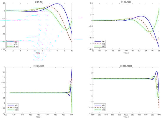
When the nonhomogeneous terms are $f\left(t\right)\ne 0$, $\sigma \left(t\right)<t$, let $\sigma \left(t\right)=t-0.2,q\left(t\right)={\displaystyle \frac{8}{3\sqrt{3}}},$ $f\left(t\right)={\displaystyle \frac{1}{t}}\ge 0$ or $f\left(t\right)=1+sint\ge 0$, where, the nonhomogeneous terms possess monotonicity and periodicity, respectively. Now, consider the following two equations

$$x^{‴}\left(t\right)+{\displaystyle \frac{8}{3\sqrt{3}}}x(t-0.2)+{\displaystyle \frac{1}{t}}=0,t\ge 1$$

(41)

$$x^{‴}\left(t\right)+{\displaystyle \frac{8}{3\sqrt{3}}}x(t-0.2)+1+sint=0,t\ge 1$$

(42)

Due to ${lim}_{t\to \infty }inf{\displaystyle \frac{8}{3\sqrt{3}}}{(t-0.2)}^{2}t>{\displaystyle \frac{2}{3\sqrt{3}}}$, both Equations (41) and (42) satisfy Theorem 2. Therefore, the solutions for these two equations exhibit an oscillatory behavior. The following plots the solutions of the two equations separately in different time intervals, as shown in Figure 1 and Figure 2.

Figure 1. Time series plot of the solution for Equation (41).

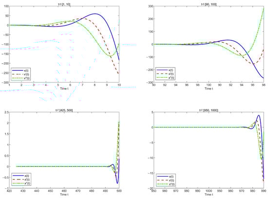
Figure 2. Time series plot of the solution to Equation (42).

Figure 1 and Figure 2 illustrate that as t gradually increases, the solutions $x\left(t\right)$ for the two equations always exhibit the behavior of crossing the zero point. And, $x^{\prime }\left(t\right),x^{″}\left(t\right)$ satisfies condition (e); this indicates that the solutions exhibit oscillatory behavior, thus verifying Theorem 2. By comparing the vertical axes of the two images, we observe that when both the nonlinear term and the delay term are identical, different types of nonhomogeneous terms exert a certain influence on the oscillation frequency and amplitude of the equation solutions. However, they do not alter the global oscillatory nature of the solutions.

Case 2.

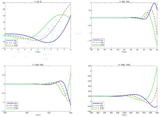
When the nonhomogeneous terms are $f\left(t\right)=0$, $\sigma \left(t\right)<t$, let $\sigma \left(t\right)=t-0.1,q\left(t\right)=2+sint\ge 0.$ i.e.,

$$x^{‴}\left(t\right)+(2+sint)x(t-0.1)=0,t\ge 0$$

(43)

Due to ${lim}_{t\to \infty }inf(2+sint){(t-0.1)}^{2}t>{\displaystyle \frac{2}{3\sqrt{3}}}$, Equation (43) satisfies Theorem 2. The solutions of the equation over different time intervals will be plotted below, as shown in Figure 3.

Figure 3. Time series plot of the solution to Equation (43).

Figure 3 illustrates that when t is sufficiently large, $x\left(t\right)$ still exhibits the behavior of crossing zero. This indicates that the solution of the equation possesses an oscillatory nature. This case demonstrates that Theorem 2 remains valid even when the nonhomogeneous term is zero.

Case 3.

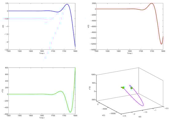
When the nonhomogeneous terms are $f\left(t\right)\ne 0$, $\sigma \left(t\right)=t$, let $f\left(t\right)=e^{-t},q\left(t\right)={\displaystyle \frac{1}{t}}.$ i.e.,

$$x^{‴}\left(t\right)+{\displaystyle \frac{1}{t}}x\left(t\right)+e^{-t}=0,t\ge 0.1$$

(44)

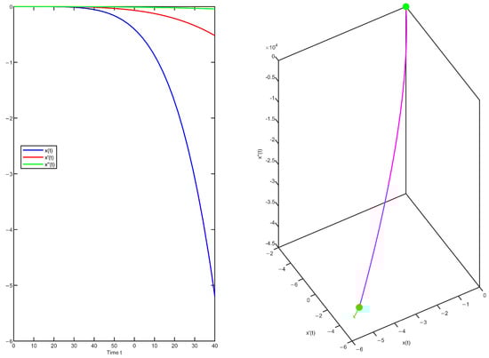
Due to ${lim}_{t\to \infty }inf{\displaystyle \frac{1}{t}}{t}^3>{\displaystyle \frac{2}{3\sqrt{3}}}$, Equation (44) satisfies Theorem 2. When the equation does not include a delay term, it suffices to analyze the behavior of the solution for a sufficiently large t, as shown in Figure 4.

Figure 4. Time series plot and phase portrait of the solution to Equation (44).

The three-dimensional phase diagram illustrates that the trajectory exhibits a spiraling upward trend. When t is sufficiently large, $x\left(t\right)$ still exhibits the behavior of crossing zero, and $x^{\prime }\left(t\right)<0,x^{″}\left(t\right)>0$ satisfies condition (e); therefore, the solutions for the equation are oscillatory. This case illustrates that Theorem 2 still holds when the delay term is absent.

Next, we present a counter example.

Case 4.

Let $q\left(t\right)={\displaystyle \frac{2}{t^4}},f\left(t\right)=t^2$, i.e.,

$$x^{‴}\left(t\right)+{\displaystyle \frac{2}{t^4}}x\left(t\right)+t^2=0,t\ge 0.1$$

(45)

Due to ${lim}_{t\to \infty }inf{\displaystyle \frac{2}{t^4}}{t}^3<{\displaystyle \frac{2}{3\sqrt{3}}}$, the equation does not satisfy Theorem 2. Since condition (34) guarantees the oscillation of Equation (33) sufficiently but not necessarily, it cannot be determined whether the solutions of Equation (45) are oscillatory. Next, we plot the solutions for this equation as shown in Figure 5.

Figure 5. Time series plot and phase portrait of the solution for Equation (45).

Figure 5 illustrates that $x\left(t\right)$ is monotonically decreasing, $x^{\prime }\left(t\right),x^{″}\left(t\right)<0$ does not satisfy condition (e); therefore, this equation does not have oscillatory solutions. This case, to some extent, verifies Theorem 2.

Collectively, under the premise of $\alpha =1$, the oscillation criterion of Equation (2) was verified through Case 1. This criterion remains valid when the nonhomogeneous term is zero or in the absence of time-delay, as demonstrated in Case 2 and Case 3. Finally, a counterexample is provided. These examples collectively validate the conclusions of Theorem 2.

References

- Glass, D.S.; Jin, X.; Riedel-Kruse, I.H. Nonlinear delay differential equations and their application to modeling biological network motifs. Nat. Commun. 2021, 1, 1788. [Google Scholar] [CrossRef] [PubMed]
- Ruzgas, T.; Jankauskienė, I.; Zajančkauskas, A.; Lukauskas, M.; Bazilevičius, M.; Kaluževičiūtė, R.; Arnastauskaitė, J. Solving Linear and Nonlinear Delayed Differential Equations Using the Lambert W Function for Economic and Biological Problems. Mathematics 2024, 17, 2760. [Google Scholar] [CrossRef]
- Alrebdi, R.; Al-Jeaid, H.K. Accurate solution for the Pantograph delay differential equation via Laplace transform. Mathematics 2023, 9, 2031. [Google Scholar] [CrossRef]
- Yan, J.; Yang, X.; Luo, X.; Guan, X. Dynamic gain control of teleoperating cyber-physical system with time-varying delay. Nonlinear. Dyn. 2019, 95, 3049–3062. [Google Scholar] [CrossRef]
- Fu, J.; Dai, Z.; Yang, Z.; Lai, J.; Yu, M. Time delay analysis and constant time-delay compensation control for MRE vibration control system with multiple-frequency excitation. Smart. Mater. Struct. 2019, 1, 014001. [Google Scholar] [CrossRef]
- Zhou, W.; Huang, C.; Xiao, M.; Cao, J. Hybrid tactics for bifurcation control in a fractional-order delayed predator–prey model. Phys. A 2019, 515, 183–191. [Google Scholar] [CrossRef]
- Guerrini, L.; Krawiec, A.; Szydłowski, M. Bifurcations in an economic growth model with a distributed time delay transformed to ODE. Nonlinear. Dyn. 2020, 2, 1263–1279. [Google Scholar] [CrossRef]
- Li, T.; Han, Z.; Sun, Y.; Zhao, Y. Asymptotic behavior of solutions for third-order half-linear delay dynamic equations on time scales. J. Appl. Math. Comput. 2011, 1, 333–346. [Google Scholar] [CrossRef]
- Chatzarakis, G.E.; Džurina, J.; Jadlovská, I. Oscillatory and asymptotic properties of third-order quasilinear delay differential equations. J. Inequal. Appl. 2019, 2019, 23. [Google Scholar] [CrossRef]
- Rakkiyappan, R.; Udhayakumar, K.; Velmurugan, G.; Cao, J.; Alsaedi, A. Stability and Hopf bifurcation analysis of fractional-order complex-valued neural networks with time delays. Adv. Differ. Equ.-Ny. 2017, 2017, 225. [Google Scholar] [CrossRef]
- Huang, X.; Deng, X.H. Properties of third-order nonlinear delay dynamic equations with positive and negative coefficients. Adv. Differ. Equ.-Ny. 2019, 2019, 292. [Google Scholar] [CrossRef]
- Shi, Y.; Han, Z.; Hou, C. Oscillation criteria for third order neutral Emden–Fowler delay dynamic equations on time scales. J. Appl. Math. Comput. 2017, 55, 175–190. [Google Scholar] [CrossRef]
- Domoshnitsky, A.; Shemesh, S.; Sitkin, A.; Yakovi, E.; Yavich, R. Stabilization of third-order differential equation by delay distributed feedback control. J. Inequal. Appl. 2018, 2018, 341. [Google Scholar] [CrossRef] [PubMed]
- Gao, L.; Zhang, Q.; Liu, S. Oscillatory behavior of third-order nonlinear delay dynamic equations on time scales. J. Comput. Appl. Math. 2014, 256, 104–113. [Google Scholar] [CrossRef]
- Yang, H.; Chen, Y. Positive periodic solutions for third-order ordinary differential equations with delay. Adv. Differ. Equ.-Ny. 2018, 2018, 270. [Google Scholar] [CrossRef]
- Zhang, Q.; Gao, L.; Yu, Y. Oscillation criteria for third-order neutral differential equations with continuously distributed delay. Appl. Math. Lett. 2012, 10, 1514–1519. [Google Scholar] [CrossRef]
- Zafer, A.; Dahiya, R.S. Oscillatory and asymptotic behavior of solutions of third order delay differential equations with forcing terms. Differ. Equ. Dyn. Syst. 1993, 2, 123–136. [Google Scholar]
- Hanan, M. Oscillation criteria for third order differential equations. Pacific J. Math. 1961, 11, 919–944. [Google Scholar] [CrossRef]
- Philos ch, G. On the existence of non-oscillatory solutions tending to zero at ∞ for differential equation with positive delay. Arch. Math. 1981, 1, 168–178. [Google Scholar] [CrossRef]
- Erbe, L. Oscillation criteria forbsecond order nonlinear delay equations. Canad. Math. Bull. 1973, 16, 49–56. [Google Scholar] [CrossRef]
- Kiguradze, I.T. On the oscilation of solutions of the equation . Math. Sb. 1964, 2, 172–187. [Google Scholar]
Disclaimer/Publisher’s Note: The statements, opinions and data contained in all publications are solely those of the individual author(s) and contributor(s) and not of MDPI and/or the editor(s). MDPI and/or the editor(s) disclaim responsibility for any injury to people or property resulting from any ideas, methods, instructions or products referred to in the content. |
© 2025 by the authors. Licensee MDPI, Basel, Switzerland. This article is an open access article distributed under the terms and conditions of the Creative Commons Attribution (CC BY) license (https://creativecommons.org/licenses/by/4.0/).