A New Class of Probability Distributions via Half-Elliptical Functions

Abstract

In this paper, we develop a new family of distributions supported on a bounded interval with a probability density function that is constructed from two elliptical arcs. The distribution can take on a variety of shapes and has three basic parameters: minimum, maximum, and mode. Compared to classical bounded distributions such as the beta and triangular distributions, the proposed semi-elliptical family offers greater flexibility in capturing diverse shapes of distributions, in symmetric and asymmetric settings. Its construction from elliptical arcs enables smoother transitions and more natural tail behaviors, making it suitable for applications where classical models may exhibit rigidity or over-simplicity. We give general expression for the density and distribution function of the new distribution. Properties of this distribution are studied and parameter estimation is discussed. Monte Carlo simulation results show the performance of our estimators under many sets of situations. Furthermore, we show the advantages of our distribution over the commonly used triangular distribution in approximating beta distributions.

1. Introduction

The topic of continuous distributions on a bounded interval is an important aspect of statistical theory and applications. In recent years, many researchers have focused their attention on developing such distributions and their applications [1,2,3,4,5,6,7]. Beta distribution is one of the most popular bounded distributions and is useful in many areas of application because it provides a rich family of distributional shapes over some finite interval [8,9,10]. Researchers developed suitable substitutes of the beta distribution over the years. For instance, the triangular distribution has been investigated by [11] as a proxy for the beta distribution in risk analysis. Many extensions have been proposed over the years. The trapezoidal distribution was constructed by adding an additional horizontal line segment in the middle and thus provides a more flexible distribution. It was used to model the duration and the form of a phenomenon which may be represented by three stages, a growth stage, a stable stage, and a decline stage, in [12]. Ref. [13] developed a new family of distributions named the two-sided power distribution and discussed its parameter estimation. Ref. [14] introduced another class of distributions called the polygonal distributions constructed from finite mixtures of the triangular distributions. Ref. [15] proposed the general segmented distributions constructed from a finite number of line segments. Ref. [16] introduced the unit-Birnbaum–Saunders distributions, which arose from the Birnbaum–Saunders distribution by the logarithmic transformation. This distribution can be considered an alternative to the beta distribution, as it exhibited decreasing, upside-down bathtub, and then bathtub-shaped density. Ref. [6] proposed the unit-half-normal distribution, which represents a power alternative to the beta distribution.

Two landmark references that comprehensively reviewed and classified bounded distributions were [1,10]. Ref. [10] provided an extensive treatment of the beta distribution and its generalizations, highlighting its probabilistic structure, estimation methods, and applications. While the beta family was shown to be flexible, the monograph noted its limitations in the complexity of some generalizations and a lack of connection to geometrically interpretable shapes. On the other hand, Ref. [1] extended the conversation by presenting a rich variety of alternative bounded distributions beyond the beta, including triangular, two-sided power, and generalized trapezoidal distributions. However, while this survey provided broad coverage, it emphasized analytical tractability and did not focus on the smoothness or visual interpretability of these shapes, often relying on piecewise linear components. Moreover, their discussion of estimation was primarily theoretical, with little exploration of fit quality compared to simpler or more natural geometric alternatives.

Motivated by these gaps in existing literature and applications, this paper introduces a new class of distributions using two elliptical arcs joined over a bounded interval. We term this the bi-elliptic distribution. Similar to the triangular distribution, it is a unimodal distribution with three parameters: the minimal value a, the maximal value b, and the mode m. However, unlike many distributions surveyed in [1,10], our proposed family aims to combine flexibility, smoothness, and interpretability in a single framework.

While the beta and triangular distributions are commonly used to model data on a bounded interval, they may lack the geometric smoothness and tail flexibility required in certain applications. For instance, the triangular distribution imposes linear density segments, which may not adequately reflect smooth real-world phenomena. The beta distribution is more flexible but requires careful parameter tuning to control skewness and modality, and its density may not always resemble familiar geometric shapes. In contrast, our proposed semi-elliptical distributions are constructed from two joined elliptical arcs, allowing for naturally smooth, symmetric (or asymmetric) densities with intuitive geometric interpretations. This structure facilitates better modeling of data with semi-elliptical characteristics and improves interpretability in applied contexts such as reliability analysis or physical measurements with inherent bounds.

The proposed distribution has several advantages in probability modeling. First, it is differentiable at all points over its support. Unlike the triangular distribution and other similar truncated distributions, the density function of the bi-elliptic distribution is differentiable everywhere in its domain, making it a better choice analytically. Second, the proposed distribution has a flatter shape around its mode, making it a better modeling choice for certain physical and social science phenomena of interest. For instance, small businesses usually experience slow growth, plateau, and decline when they reach the stage of maturity [17]. Third, the three parameters in the distribution provide large flexibility in modeling. Particularly, the distribution can be negatively skewed, positively skewed, or symmetric. Finally, similar to the triangular distribution, the bi-elliptic distribution is based on a knowledge of the minimum, maximum, and most common modal value, enabling it to work when data are limited. For example, it can be used in quantitatively analyzing the uncertainty of three-point-estimate problems [18].

This paper is organized as follows. Section 2 presents the bi-elliptic distribution and its basic properties. In Section 3, the maximum likelihood estimation (MLE) procedure for bi-elliptic distributions is discussed. Section 4 presents a wide range of Monte Carlo simulation results for parameter estimation. Section 5 compares the triangular distribution and the proposed bi-elliptic distribution in fitting data drawn from a range of beta distributions. Finally, we provide some concluding remarks in Section 6.

2. The Bi-Elliptic Distribution

2.1. Definition

We define a bi-elliptic probability density function (PDF) over a finite interval $[a,b]$ with mode at m, where $a\le m\le b$. The PDF is constructed by smoothly joining two quarter-elliptical arcs—each representing half of the upper half of an ellipse—on either side of the mode.

Let X be a random variable with a probability density function given by

$$f(x;a,b,m)=\left\{\begin{array}{cc}k·\sqrt{1-{\left({\displaystyle \frac{x-m}{m-a}}\right)}^2},\hfill & \mathrm{if}a\le x\le m,\hfill \\ k·\sqrt{1-{\left({\displaystyle \frac{x-m}{b-m}}\right)}^2},\hfill & \mathrm{if}m<x\le b,\hfill \end{array}\right.$$

(1)

where $k>0$ is a normalizing constant. This function is shaped by two quarter-elliptical curves centered at the mode m, with horizontal stretches over $[a,m]$ and $[m,b]$, respectively.

Normalization Condition

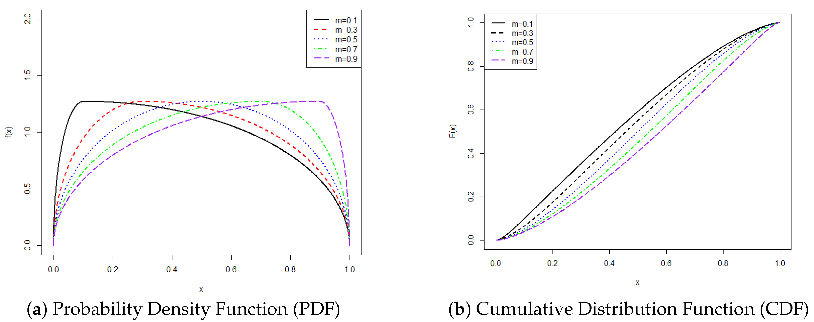
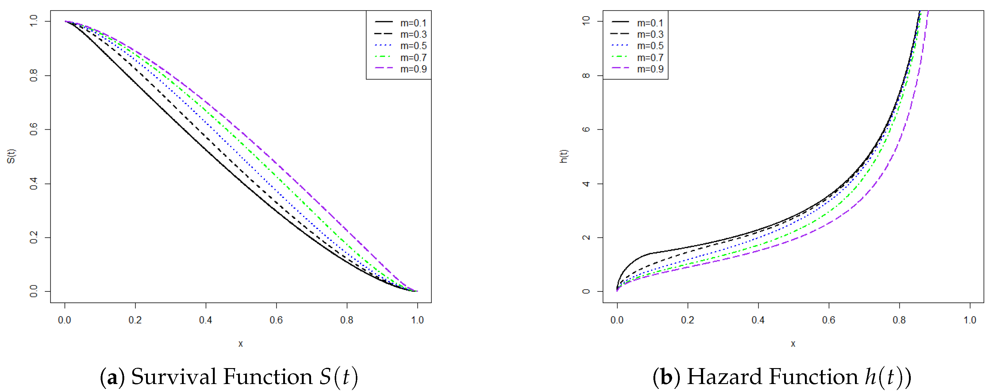
To ensure that $f\left(x\right)$ is a valid PDF, we require:

$${\int }_a^{b}f\left(x\right)dx=1.$$

We compute the integral in two parts:

$${\int }_a^{b}f\left(x\right)dx={\int }_a^{m}k·\sqrt{1-{\left({\displaystyle \frac{x-m}{m-a}}\right)}^2}dx+{\int }_m^{b}k·\sqrt{1-{\left({\displaystyle \frac{x-m}{b-m}}\right)}^2}dx.$$

For the first part, let $u={\displaystyle \frac{x-m}{m-a}}\Rightarrow dx=(m-a)du$, and as x goes from a to m, u goes from $-1$ to 0:

$${\int }_a^{m}k·\sqrt{1-{\left({\displaystyle \frac{x-m}{m-a}}\right)}^2}dx=k(m-a){\int }_{-1}^0\sqrt{1-u^2}du.$$

For the second part, let $v={\displaystyle \frac{x-m}{b-m}}\Rightarrow dx=(b-m)dv$, and as x goes from m to b, v goes from 0 to 1:

$${\int }_m^{b}k·\sqrt{1-{\left({\displaystyle \frac{x-m}{b-m}}\right)}^2}dx=k(b-m){\int }_0^1\sqrt{1-v^2}dv.$$

Note that:

$${\int }_{-1}^0\sqrt{1-u^2}du={\int }_0^1\sqrt{1-v^2}dv={\displaystyle \frac{\pi }{4}}.$$

Therefore,

$$\begin{array}{cc}\hfill {\int }_a^{b}f\left(x\right)dx& =k(m-a)·{\displaystyle \frac{\pi }{4}}+k(b-m)·{\displaystyle \frac{\pi }{4}}\hfill \\ \hfill & =k·{\displaystyle \frac{\pi }{4}}·\left[(m-a)+(b-m)\right]\hfill \\ \hfill & =k·{\displaystyle \frac{\pi }{4}}·(b-a).\hfill \end{array}$$

To normalize $f\left(x\right)$, set:

$$k·{\displaystyle \frac{\pi }{4}}·(b-a)=1\Rightarrow k={\displaystyle \frac{4}{\pi (b-a)}}.$$

The normalized bi-elliptic distribution is:

$$f\left(x\right)=\left\{\begin{array}{cc}{\displaystyle \frac{4}{\pi (b-a)}}·\sqrt{1-{\left({\displaystyle \frac{x-m}{m-a}}\right)}^2},\hfill & \mathrm{if}a\le x\le m,\hfill \\ {\displaystyle \frac{4}{\pi (b-a)}}·\sqrt{1-{\left({\displaystyle \frac{x-m}{b-m}}\right)}^2},\hfill & \mathrm{if}m<x\le b.\hfill \end{array}\right.$$

(2)

This function consists of two quarter-elliptical arcs joined at the mode m, continuous and differentiable on $(a,b)$, symmetric about the mode if $m={\displaystyle \frac{a+b}{2}}$, and integrates to 1. It thus satisfies the conditions for a valid probability density function.

The random variable X is said to have a bi-elliptic distribution, $E(a,b,m)$, $a<m<b$. Here, a is the lower limit, b is the upper limit, and m is the mode. In addition, bi-elliptic distributions also include two extreme cases when $m=a$ or $m=b$:

$$\begin{array}{cc}\hfill f(x;a,b,m)& ={\displaystyle \frac{4}{\pi (b-a)}}·\sqrt{1-{\left({\displaystyle \frac{x-b}{b-a}}\right)}^2},a\le x\le b,ifm=b,\hfill \end{array}$$

(3)

$$\begin{array}{cc}\hfill f(x;a,b,m)& ={\displaystyle \frac{4}{\pi (b-a)}}·\sqrt{1-{\left({\displaystyle \frac{x-a}{b-a}}\right)}^2},a\le x\le b,ifm=a.\hfill \end{array}$$

(4)

We call the bi-elliptic distribution with $a=0$ and $b=1$ the standard bi-elliptic distribution. The PDF of a standard elliptic distribution with mode m is

$$f(x;0,1,m)=\left\{\begin{array}{cc}{\displaystyle \frac{4}{\pi }}·\sqrt{1-{\left({\displaystyle \frac{x-m}{m}}\right)}^2},\hfill & \mathrm{if}0\le x\le m,\hfill \\ {\displaystyle \frac{4}{\pi }}·\sqrt{1-{\left({\displaystyle \frac{x-m}{1-m}}\right)}^2},\hfill & \mathrm{if}m<x\le 1.\hfill \end{array}\right.$$

(5)

For any bi-elliptic distribution $X\sim E(a,b,m)$, the following property holds:

$$Y={\displaystyle \frac{X-a}{b-a}}\sim E\left(0,1,{\displaystyle \frac{m-a}{b-a}}\right).$$

(6)

This property can be easily proven using the change-of-variable technique.

Figure 1a provides the density plots of examples of symmetric, positively and negatively skewed $E(0,1,m)$ distributions for different choices of m values. As we can see, the distribution is right-skewed if $m<0.5$; it is left-skewed if $m>0.5$; the distribution is symmetric if $m=0.5$.

The cumulative distribution function of an $E(a,b,m)$ distribution can be derived from Equation (1) and is given below:

$$F\left(x\right)=\left\{\begin{array}{cc}0,\hfill & x<a,\hfill \\ {\displaystyle \frac{2}{\pi (b-a)}}\left[(x-m)\sqrt{1-{\left({\displaystyle \frac{x-m}{m-a}}\right)}^2}+(m-a){sin}^{-1}\left({\displaystyle \frac{x-m}{m-a}}\right)\right]+{\displaystyle \frac{m-a}{b-a}},\hfill & a\le x\le m,\hfill \\ {\displaystyle \frac{2}{\pi (b-a)}}\left[(x-m)\sqrt{1-{\left({\displaystyle \frac{x-m}{b-m}}\right)}^2}+(b-m){sin}^{-1}\left({\displaystyle \frac{x-m}{b-m}}\right)\right]+{\displaystyle \frac{m-a}{b-a}},\hfill & m<x\le b,\hfill \\ 1,\hfill & x>b.\hfill \end{array}\right.$$

(7)

Figure 1b provides plots of the distribution function for examples of symmetric, positively and negatively skewed $E(0,1,m)$ distributions for different choices of m values.

2.2. Properties

The survival function $S\left(t\right)$ of the bi-elliptic distribution is defined as $S\left(t\right)=1-F\left(t\right)$, where $F\left(t\right)$ is the cumulative distribution function (CDF). For parameters $a<m<b$:

$$S\left(t\right)=\left\{\begin{array}{cc}1,\hfill & t<a,\hfill \\ {\displaystyle \frac{b-m}{b-a}}-{\displaystyle \frac{2}{\pi (b-a)}}\left[(t-m)\sqrt{1-{\left({\displaystyle \frac{t-m}{m-a}}\right)}^2}+(m-a){sin}^{-1}\left({\displaystyle \frac{t-m}{m-a}}\right)\right],\hfill & a\le t\le m,\hfill \\ {\displaystyle \frac{b-m}{b-a}}-{\displaystyle \frac{2}{\pi (b-a)}}\left[(t-m)\sqrt{1-{\left({\displaystyle \frac{t-m}{b-m}}\right)}^2}+(b-m){sin}^{-1}\left({\displaystyle \frac{t-m}{b-m}}\right)\right],\hfill & m\le t\le b,\hfill \\ 0,\hfill & t>b.\hfill \end{array}\right.$$

(8)

The survival function $S\left(t\right)$ decreases smoothly from 1 (at $t=a$) to 0 (at $t=b$).

The hazard rate function $h\left(t\right)$ is defined as $h\left(t\right)={\displaystyle \frac{f\left(t\right)}{S\left(t\right)}}$, where $f\left(t\right)$ is the probability density function (PDF):

$$h\left(t\right)=\left\{\begin{array}{cc}0,\hfill & t<a\mathrm{or}t>b,\hfill \\ {\displaystyle \frac{\frac{4}{\pi (b-a)}\sqrt{1-{\left(\frac{m-t}{m-a}\right)}^2}}{\frac{b-m}{b-a}-\frac{2}{\pi (b-a)}\left[(t-m)\sqrt{1-{\left(\frac{t-m}{m-a}\right)}^2}+(m-a){sin}^{-1}\left(\frac{t-m}{m-a}\right)\right]}},\hfill & a\le t\le m,\hfill \\ {\displaystyle \frac{\frac{4}{\pi (b-a)}\sqrt{1-{\left(\frac{t-m}{b-m}\right)}^2}}{\frac{b-m}{b-a}-\frac{2}{\pi (b-a)}\left[(t-m)\sqrt{1-{\left(\frac{t-m}{b-m}\right)}^2}+(b-m){sin}^{-1}\left(\frac{t-m}{b-m}\right)\right]}},\hfill & m\le t\le b.\hfill \end{array}\right.$$

(9)

Figure 2a provides plots of the survival function for examples of symmetric, positively and negatively skewed $E(0,1,m)$ distributions for different choices of m values. Figure 2b provides plots of the corresponding hazard functions.

For any bi-elliptic distribution, m is the mode and the $\alpha$-quantile $Q_{\alpha }\left(x\right)$ with $\alpha ={\displaystyle \frac{m-a}{b-a}}$. The median of a bi-elliptic distribution $E(a,b,m)$ is the unique real value x for which $F\left(x\right)=0.5$. There is no general closed-form expression for the median. However, for symmetric cases when $m=(a+b)/2$, the median is the mode m.

The moment generating function (MGF) is given by:

$$M_X\left(t\right)=\mathbb{E}\left[e^{tX}\right]={\displaystyle \frac{4}{\pi (b-a)}}\left[{\int }_a^m{e}^{tx}\sqrt{1-{\left({\displaystyle \frac{x-a}{m-a}}\right)}^2}dx+{\int }_m^b{e}^{tx}\sqrt{1-{\left({\displaystyle \frac{x-b}{b-m}}\right)}^2}dx\right],$$

which can be computed using the following substitutions:

• For $x\in [a,m]$: let $x=a+(m-a)sin\theta$, so $dx=(m-a)cos\theta d\theta$, $\theta \in [0,{\displaystyle \frac{\pi }{2}}]$.
• For $x\in [m,b]$: let $x=b+(m-b)sin\varphi$, so $dx=(b-m)cos\varphi d\varphi$, $\varphi \in \left[-{\displaystyle \frac{\pi }{2}},0\right]$.

We obtain

$$\begin{array}{cc}\hfill M_X\left(t\right)& ={\displaystyle \frac{4}{\pi (b-a)}}\left[{\int }_0^{{\displaystyle \frac{\pi }{2}}}{e}^{t(a+(m-a)sin\theta )}(m-a){cos}^2\theta d\theta +{\int }_{-{\displaystyle \frac{\pi }{2}}}^0{e}^{t(b+(m-b)sin\varphi )}(b-m){cos}^2\varphi d\varphi \right]\hfill \\ \hfill & ={\displaystyle \frac{4(m-a)}{\pi (b-a)}}{\int }_0^{{\displaystyle \frac{\pi }{2}}}{e}^{t(a+(m-a)sin\theta )}{cos}^2\theta d\theta +{\displaystyle \frac{4(b-m)}{\pi (b-a)}}{\int }_{-{\displaystyle \frac{\pi }{2}}}^0{e}^{t(b+(m-b)sin\varphi )}{cos}^2\varphi d\varphi .\hfill \end{array}$$

(10)

The first four moments and the variance of $E(a,b,m)$ can be obtained from the density function (1) and simplified as follows:

$$\begin{array}{cc}\hfill E\left(X\right)& =\mu =m+{\displaystyle \frac{4(a+b-2m)}{3\pi }},\hfill \end{array}$$

(11)

$$\begin{array}{cc}\hfill E\left(X^2\right)& =m^2+{\displaystyle \frac{8m(a+b-2m)}{3\pi }}+{\displaystyle \frac{{(a-m)}^2+{(b-m)}^2}{4}},\hfill \end{array}$$

(12)

$$\begin{array}{cc}\hfill E\left(X^3\right)& ={\displaystyle \frac{4}{\pi }}\left[{\displaystyle \frac{\pi m^3}{4}}+m^2(a+b-2m)+{\displaystyle \frac{3\pi m[{(a-m)}^2+{(b-m)}^2]}{16}}+{\displaystyle \frac{2[{(b-m)}^3-{(m-a)}^3]}{15}}\right],\hfill \end{array}$$

(13)

$$\begin{array}{cc}E\left(X^4\right)\hfill & ={\displaystyle \frac{4}{\pi (b-a)}}\left\{{\displaystyle \frac{\pi m^4}{4}}(b-a)+{\displaystyle \frac{4m^3}{3}}\left[{(b-m)}^2-{(m-a)}^2\right]+{\displaystyle \frac{3\pi m^2}{8}}\left[{(b-m)}^3-{(m-a)}^3\right]\right.\hfill \\ \hfill & \left.+{\displaystyle \frac{8m}{15}}\left[{(b-m)}^4-{(m-a)}^4\right]+{\displaystyle \frac{\pi }{32}}\left[{(b-m)}^5+{(m-a)}^5\right]\right\}.\hfill \end{array}$$

(14)

Higher-order moments $E\left(X^r\right)$ are guaranteed to exist since the support $[a,b]$ is bounded. However, closed-form expression for $r>4$ is very complicated.

The variance is given by

$$Var\left(X\right)={\sigma }^2={\displaystyle \frac{{(a-m)}^2+{(b-m)}^2}{4}}-{\displaystyle \frac{16}{9{\pi }^2}}{(a+b-2m)}^2.$$

(15)

The detailed calculations of the moments and variance are provided in Appendix A.

The explicit expressions for the skewness and the kurtosis are very complicated. We present them in terms of the moments and note the complexity:

$$\begin{array}{c}\hfill {\gamma }_1={\displaystyle \frac{E{(X-\mu )}^3}{{\sigma }^3}}={\displaystyle \frac{E(X^3-3\mu E\left(X^2\right)+2{\mu }^3}{{\sigma }^3}},\end{array}$$

(16)

$$\begin{array}{c}\hfill {\gamma }_2={\displaystyle \frac{E{(X-\mu )}^4}{{\sigma }^4}}={\displaystyle \frac{E\left(X^4\right)-4\mu E\left(X^3\right)+6{\mu }^{2}E\left(X^2\right)-3{\mu }^4}{{\sigma }^4}}.\end{array}$$

(17)

The Rényi entropy of order $\alpha$,

$$H_{\alpha }={\displaystyle \frac{1}{1-\alpha }}log\left({\int }_a^{b}f{\left(x\right)}^{\alpha }dx\right),$$

for the bi-elliptic distribution is

$$\begin{array}{cc}\hfill H_{\alpha }& ={\displaystyle \frac{1}{1-\alpha }}log\left({\left({\displaystyle \frac{4}{\pi (b-a)}}\right)}^{\alpha }(b-a)·{\displaystyle \frac{\sqrt{\pi }}{2}}{\displaystyle \frac{\Gamma \left(\frac{\alpha +1}{2}\right)}{\Gamma \left(\frac{\alpha +3}{2}\right)}}\right).\hfill \end{array}$$

(18)

Further simplification gives:

$$\begin{array}{c}\hfill H_{\alpha }={\displaystyle \frac{1}{1-\alpha }}\left[(2\alpha -1)log2+\left({\displaystyle \frac{1}{2}}-\alpha \right)log\pi +(1-\alpha )log(b-a)+log{\displaystyle \frac{\Gamma \left(\frac{\alpha +1}{2}\right)}{\Gamma \left(\frac{\alpha +3}{2}\right)}}\right].\end{array}$$

(19)

Surprisingly, the Rényi entropy of order $\alpha$ does not depend on the mode m and only depends on the interval length $b-a$ and the parameter $\alpha$. A step-by-step derivation is provided in Appendix A.

The mean residual life at time t is defined as

$$MRL\left(t\right)={\displaystyle \frac{1}{S\left(t\right)}}{\int }_a^b(x-t)f\left(x\right)dx,$$

(20)

where $S\left(t\right)$ is the survival function. The integral involves elliptic integrals and does not simplify to elementary functions.

The r-th incomplete moment up to $c\in [a,b]$ is

$${\mu }_r\left(c\right)={\int }_a^c{x}^{r}f\left(x\right)dx=\left\{\begin{array}{cc}{\displaystyle \frac{4}{\pi (b-a)}}{\int }_a^c{x}^r\sqrt{1-{\left({\displaystyle \frac{m-x}{m-a}}\right)}^2}dx,\hfill & a\le c<m,\hfill \\ {\mu }_r\left(m\right)+{\displaystyle \frac{4}{\pi (b-a)}}{\int }_m^c{x}^r\sqrt{1-{\left({\displaystyle \frac{x-m}{b-m}}\right)}^2}dx,\hfill & m\le c\le b.\hfill \end{array}\right.$$

(21)

These integrals resemble moments of a semicircular distribution. However, closed-form expressions for general r and c require special functions and are not elementary.

Let $X_1,X_2,\dots ,X_n$ be a random sample from the bi-elliptic distribution with parameters a, m, and b. The k-th order statistic, denoted $X_{\left(k\right)}$, has a probability density function (PDF) given by:

$$f_{X_{\left(k\right)}}\left(x\right)={\displaystyle \frac{n!}{(k-1)!(n-k)!}}{\left[F\left(x\right)\right]}^{k-1}{\left[1-F\left(x\right)\right]}^{n-k}f\left(x\right),$$

where:

• $F\left(x\right)$ is the cumulative distribution function (CDF) of the bi-elliptic distribution;
• $f\left(x\right)$ is the probability density function (PDF) of the bi-elliptic distribution;
• $k\in \{1,2,\dots ,n\}$ denotes the position of the ordered statistic.

For the bi-elliptic distribution with support $[a,b]$ and mode m, the PDF of $X_{\left(k\right)}$ is piecewise-defined due to the piecewise nature of $F\left(x\right)$ and $f\left(x\right)$:

• For $x\in [a,m]$:

  $$\begin{array}{cc}\hfill f_{X_{\left(k\right)}}\left(x\right)& ={\displaystyle \frac{n!}{(k-1)!(n-k)!}}\hfill \\ \hfill & \times {\left[{\displaystyle \frac{2}{\pi }}·{\displaystyle \frac{m-a}{b-a}}\left({\displaystyle \frac{\pi }{2}}-{sin}^{-1}\left({\displaystyle \frac{m-x}{m-a}}\right)-{\displaystyle \frac{m-x}{m-a}}\sqrt{1-{\left({\displaystyle \frac{m-x}{m-a}}\right)}^2}\right)\right]}^{k-1}\hfill \\ \hfill & \times {\left[1-F\left(x\right)\right]}^{n-k}·{\displaystyle \frac{4}{\pi (b-a)}}\sqrt{1-{\left({\displaystyle \frac{m-x}{m-a}}\right)}^2}.\hfill \end{array}$$
• For $x\in [m,b]$:

  $$\begin{array}{cc}\hfill f_{X_{\left(k\right)}}\left(x\right)& ={\displaystyle \frac{n!}{(k-1)!(n-k)!}}{\left[F\left(x\right)\right]}^{k-1}\hfill \\ \hfill & \times {\left[{\displaystyle \frac{2}{\pi }}·{\displaystyle \frac{b-m}{b-a}}\left({\displaystyle \frac{\pi }{2}}-arcsin\left({\displaystyle \frac{x-m}{b-m}}\right)-{\displaystyle \frac{x-m}{b-m}}\sqrt{1-{\left({\displaystyle \frac{x-m}{b-m}}\right)}^2}\right)\right]}^{n-k}\hfill \\ \hfill & \times {\displaystyle \frac{4}{\pi (b-a)}}\sqrt{1-{\left({\displaystyle \frac{x-m}{b-m}}\right)}^2}.\hfill \end{array}$$

Closed-form expressions for $f_{X_{\left(k\right)}}\left(x\right)$ are intractable due to the nonlinearity of $F\left(x\right)$ and $f\left(x\right)$. Numerical methods or Monte Carlo simulations are recommended for evaluation.

3. Parameter Estimation

3.1. Maximum Likelihood Estimation

For a random sample $\mathbf{X}=(X_1,\dots ,X_n)$ of size n from an $E(a,b,m)$ distribution, let the order statistics be $X_{\left(1\right)}<X_{\left(2\right)}<\dots <X_{\left(n\right)}$. Using expression (1), the likelihood function for $\mathbf{X}$ can be obtained as follows:

$$L(\mathbf{X};a,b,m)={\left[{\displaystyle \frac{4}{\pi (b-a)}}\right]}^{n}H(\mathbf{X};a,b,m),$$

(22)

where

$$H(\mathbf{X};a,b,m)=\prod _{i=1}^s\sqrt{1-{\left({\displaystyle \frac{X_{\left(i\right)}-m}{m-a}}\right)}^2}·\prod _{i=s+1}^n\sqrt{1-{\left({\displaystyle \frac{X_{\left(i\right)}-m}{b-m}}\right)}^2},$$

(23)

$X_{\left(0\right)}\equiv a,X_{(n+1)}\equiv b$ and s is implicitly defined by $X_{\left(s\right)}\le m\le X_{(s+1)}.$

From Equation (22), the log-likelihood function can be written as:

$$\begin{array}{cc}\hfill logL(\mathbf{X};a,b,m)& =nlog\left({\displaystyle \frac{4}{\pi (b-a)}}\right)+{\displaystyle \frac{1}{2}}\sum _{i=1}^{s}log\left(1-{\left({\displaystyle \frac{X_{\left(i\right)}-m}{m-a}}\right)}^2\right)\hfill \\ \hfill & +{\displaystyle \frac{1}{2}}\sum _{i=s+1}^{n}log\left(1-{\left({\displaystyle \frac{X_{\left(i\right)}-m}{b-m}}\right)}^2\right),\hfill \end{array}$$

(24)

which is equivalent to:

$$\begin{array}{cc}\hfill logL(\mathbf{X};a,b,m)& =nlog{\displaystyle \frac{4}{\pi }}-nlog(b-a)\hfill \\ \hfill & +{\displaystyle \frac{1}{2}}\sum _{i=1}^s\left[log\left(X_{\left(i\right)}-a\right)+log\left(2m-a-X_{\left(i\right)}\right)-2log(m-a)\right]\hfill \\ \hfill & +{\displaystyle \frac{1}{2}}\sum _{i=s+1}^n\left[log\left(b-X_{\left(i\right)}\right)+log\left(b+X_{\left(i\right)}-2m\right)-2log(b-m)\right].\hfill \end{array}$$

(25)

We have the following partial derivatives:

$$\begin{array}{cc}\hfill {\displaystyle \frac{\partial logL}{\partial a}}& ={\displaystyle \frac{n}{b-a}}+{\displaystyle \frac{1}{2}}\sum _{i=1}^s\left[{\displaystyle \frac{1}{a-X_{\left(i\right)}}}+{\displaystyle \frac{1}{a+X_{\left(i\right)}-2m}}-{\displaystyle \frac{2}{a-m}}\right],\hfill \end{array}$$

(26)

$$\begin{array}{cc}\hfill {\displaystyle \frac{\partial logL}{\partial b}}& =-{\displaystyle \frac{n}{b-a}}+{\displaystyle \frac{1}{2}}\sum _{i=s+1}^n\left[{\displaystyle \frac{1}{b-X_{\left(i\right)}}}+{\displaystyle \frac{1}{b+X_{\left(i\right)}-2m}}-{\displaystyle \frac{2}{b-m}}\right],\hfill \end{array}$$

(27)

$$\begin{array}{cc}\hfill {\displaystyle \frac{\partial logL}{\partial m}}& =-\sum _{i=1}^s\left[{\displaystyle \frac{1}{a+X_{\left(i\right)}-2m}}-{\displaystyle \frac{1}{a-m}}\right]-\sum _{i=s+1}^n\left[{\displaystyle \frac{1}{b+X_{\left(i\right)}-2m}}-{\displaystyle \frac{1}{b-m}}\right].\hfill \end{array}$$

(28)

Because the log-likelihood leads to a set of nonlinear and interdependent score equations in terms of the parameters a, b, and m, analytical solutions are intractable and numerical methods are required.

Due to the complexity of the bi-elliptic density function, the log-likelihood function is non-concave in general with respect to all three parameters, especially when all three are treated as free parameters. However, the uniqueness of the MLE can be investigated in constrained settings. If a and b are known, the log-likelihood becomes a function of a single parameter m. In this one-parameter case, the log-likelihood function is typically unimodal with respect to m and exhibits a unique maximum, provided the data are not degenerate. When a, b, and m are all estimated jointly, the parameter space is more complex. However, by enforcing the natural order constraints $a<m<b$ and bounding the support, the optimization problem becomes well posed. The likelihood surface may contain local optima, but in practice, the global maximum is typically identifiable when the sample is sufficiently large and the data cover the full support.

3.2. One-Parameter Maximum Likelihood Estimation

The one-parameter case is of special interest because in some applications, there exist natural lower and upper bounds for random variables of interests. For instance, in hydrology, the reservoir yield and storage distribution has a natural upper bound, being its capacity, and a lower bound, being zero [19].

When $a=a_0$ and $b=b_0$ are fixed and known, taking the partial derivative of the log-likelihood function $logL$ with respect to m yields Equation (28), whose critical point(s) do not have an explicit form. The one-parameter maximum likelihood estimation is an optimization problem, as shown below:

$$\underset{a_0<m<b_0}{max}\left\{L(\mathbf{X};a_0,b_0,m)\right\}$$

(29)

or, equivalently,

$$\underset{a_0<m<b_0}{max}\left\{logL(\mathbf{X};a_0,b_0,m)\right\}$$

(30)

where $L(\mathbf{X};a_0,b_0,m)$ and $logL(\mathbf{X};a_0,b_0,m)$ are given by Equations (22) and (24), respectively, with a and b being replaced by $a_0$ and $b_0$. This optimization problem can be solved using numerical methods. For instance, we use Brent’s algorithm for the numerical computations, which combines linear interpolation and inverse quadratic interpolation with bisection for one-dimensional optimization problems. Interested readers may refer to [20] for more details.

3.3. Three-Parameter Maximum Likelihood Estimation

There are many cases where we have no information about the values of a, b, and m, and in such cases, we need to estimate the values of the three parameters simultaneously. The partial derivatives of the log likelihood function $logL(\mathbf{X};a,b,m)$ are derived and given in Equations (26)–(28), respectively. Again, we cannot find explicit forms for their critical values and we resort to numerical methods for finding the MLE via the log likelihood function. We have

$$\underset{S(a,b,m)}{max}\left\{logL(\mathbf{X};a,b,m)\right\}$$

(31)

where $S(a,b,m)=\{(a,m,b):a<X_{\left(1\right)},b>X_{\left(n\right)},a<m<b\}$ and $logL(\mathbf{X};a,b,m)$ is given by Equation (24). A linearly constrained optimization algorithm can be used for the numerical computation. Given a random sample, we can calculate gradients (vector of the partial derivatives with respect to a, b, and m) of the log likelihood function $logL(\mathbf{X};a,b,m)$. For a random sample $\mathbf{X}=(X_1,\dots ,X_n)$ with order statistics, $X_{\left(1\right)}<X_{\left(2\right)}<\dots <X_{\left(n\right)}$. The linear constraints on the parameters a, b, and m can be formulated as follows:

$$a<X_{\left(1\right)},b>X_{\left(n\right)},m>a,m<b.$$

Interested readers may refer to [21] for details of the linearly constrained optimization algorithm.

3.4. Numerical Implementation and Computational Considerations

This section outlines the computational framework for maximum likelihood estimation (MLE) of the bi-elliptic distribution parameters. The implementation leverages R’s core optimization tools, emphasizing reproducibility, efficiency, and robustness to address concerns about convergence, computational effort, and methodological transparency.

3.4.1. One-Parameter MLE for m

When a and b are known, the mode m is estimated by maximizing the log-likelihood function (24) over $m\in (a,b)$. This univariate optimization problem is solved using the Brent method [20], which is a robust algorithm combining parabolic interpolation and golden-section search. The Brent method is computationally efficient for univariate problems. It requires $O\left(log\right({ϵ}^{-1}$)) iterations for tolerance $ϵ$ and guarantees convergence to a local maximum within $(a,b)$.

3.4.2. Three-Parameter MLE for a, b, and m

For the joint estimation of a, b, and m, the constrOptim function with the L-BFGS-B algorithm [22] is employed, which handles box constraints via projected gradients. L-BFGS-B is a quasi-Newton method that efficiently handles bound constraints. This choice is motivated by L-BFGS-B’s ability to approximate the Hessian matrix implicitly, thus reducing computational overhead while maintaining superlinear convergence rates.

3.4.3. Comparison with Alternative Methods

The proposed MLE framework outperforms alternative approaches in both robustness and efficiency. The method of moment estimates parameters by solving $E\left(X^k\right]={\displaystyle \frac{1}{n}}\sum x_i^k$. This method faces critical limitations for bi-elliptic distribution such as intractable integrals, nonlinear equation systems, and constraint violations. The Bayesian method faces challenges for the bi-elliptic distribution since it requires specifying priors and is more computationally inefficient. In addition, it also has convergence issues.

For the bi-elliptic distribution, MLE outperforms alternative methods in accuracy, speed, and robustness while natively handling parameter constraints. Its theoretical guarantees and practical efficiency make it the unequivocal choice for parameter estimation.

4. Monte Carlo Simulations

In this section, we illustrate some previous results on one-parameter MLE and three-parameter MLE using Monte Carlo simulations. All computations are performed using the open source statistical software R-4.5.0.

For all simulations in this section, we use the Inverse Transform Sampling method to generate random samples from the bi-elliptic distribution. Here is a step-by-step overview:

• Generate uniform random numbers $u_i,u_2,\dots ,u_N$ from a uniform distribution on [0,1].
• Compute quantiles via numerical inversion: For each $u_i$, solve $F_X\left(x\right)=u_i$ numerically to find $x_i=F_X^{-1}\left(u_i\right)$, where $F{(}_X\left(x\right)$ is the bi-elliptic CDF. We used the R function uniroot() in R package: stat for implementation.
• Output samples: Collect all $x_i$ values to form the random sample $(x_1,x_2,\dots ,x_N)$.

4.1. One-Parameter MLE

For one-parameter MLE, we consider the bi-elliptic distributions where m is the only unknown parameter. For our simulation, we set $a=0$ and $b=1$.

The values of m and n used in the simulation are $m=0.1,0.3,0.5,0.7,0.9$; $n=200,400,600,$$800,1000$. This gives a total of 25 different combinations of m and n. For each fixed pair of m and n, 10,000 random samples were drawn from the corresponding bi-elliptic distribution $f(x;0,1,m)$. For each of the 10,000 random samples, we calculate the estimates of the maximum likelihood estimator using the numerical method described in the previous section. The initial value is set at 0.5. These estimates are denoted by ${\widehat{m}}_1,\dots ,{\widehat{m}}_{10,000}$. Four performance measures are used to evaluate how our method estimates the value of the parameter m: the bias, the empirical standard error (Empirical SE), the mean square error (MSE), and the root mean square error (RMSE).

Table 1. Performance measures of parameter estimation. Here, $\theta$ is the true parameter and $\widehat{\theta }$ is the estimator and ${\widehat{\theta }}_1,\dots ,{\widehat{\theta }}_k$ are the estimates. Here, ${\displaystyle \overline{\widehat{\theta }}=\frac{1}{k}\sum _{i=1}^k{\widehat{\theta }}_i}$.

Measure	Definition	Estimate
Bias	${\displaystyle E\left(\widehat{\theta }\right)-\theta }$	${\displaystyle \overline{\widehat{\theta }}-\theta }$
Empirical Standard Error (Empirical SE)	${\displaystyle E{\left[\widehat{\theta }-E\left(\widehat{\theta }\right)\right]}^2}$	${\displaystyle \sqrt{\frac{1}{k-1}\sum _{i=1}^k{\left({\widehat{\theta }}_i-\overline{\widehat{\theta }}\right)}^2}}$
Mean Square Error (MSE)	$E{(\widehat{\theta }-\theta )}^2$	${\displaystyle \frac{1}{k}\sum _{i=1}^k{({\widehat{\theta }}_i-\theta )}^2}$
Root Mean Square Error (RMSE)	$\sqrt{E{(\widehat{\theta }-\theta )}^2}$	${\displaystyle \sqrt{\frac{1}{k}\sum _{i=1}^k{({\widehat{\theta }}_i-\theta )}^2}}$

summarizes these measures.

Table 2. One-parameter estimation.

	Size	Bias	Empirical SE	MSE	RMSE
m = 0.1	200	0.0159	0.0792	0.0065	0.0808
	400	0.0088	0.0563	0.0032	0.0569
	600	0.0061	0.0514	0.0027	0.0517
	800	0.0044	0.0479	0.0023	0.0481
	1000	−0.0037	0.0451	0.0020	0.0453
m = 0.3	200	0.0072	0.1105	0.0123	0.1107
	400	0.0045	0.0785	0.0062	0.0786
	600	0.0032	0.0632	0.0040	0.0633
	800	−0.0021	0.0561	0.0031	0.0561
	1000	0.0025	0.0540	0.0029	0.0540
m = 0.5	200	0.0013	0.1179	0.0139	0.1179
	400	−0.0012	0.0838	0.0070	0.0838
	600	0.0009	0.0686	0.0047	0.0686
	800	0.0010	0.0607	0.0037	0.0607
	1000	0.0007	0.0547	0.0030	0.0547
m = 0.7	200	−0.0065	0.1097	0.0121	0.1099
	400	−0.0022	0.0761	0.0058	0.0761
	600	0.0009	0.0620	0.0038	0.0620
	800	−0.0022	0.0544	0.0030	0.0544
	1000	−0.0017	0.0487	0.0024	0.0487
m = 0.9	200	−0.0168	0.0771	0.0062	0.0789
	400	0.0078	0.0529	0.0029	0.0534
	600	−0.0044	0.0425	0.0018	0.0427
	800	0.0031	0.0371	0.0014	0.0372
	1000	−0.0026	0.0327	0.0011	0.0328

presents the simulation results for the one-parameter MLE. We have two conclusions. First, for each selected value of m, the absolute values of the biases associated with the estimator $\widehat{m}$ in estimating m have a decreasing trend as the sample size increases from 200 to 1000. The Empirical SE, MSE, and RMSE for $\widehat{m}$ in estimating m are also given and they all decrease as the sample size increases. Second, for each selected sample size n, the values of the four performance measures for different values of m are, in general, close to each other. This implies that our estimator $\widehat{m}$ has a uniform effect in estimating m for different choices of m.

4.2. Three-Parameter MLE

In the three-parameter MLE, all three parameters a, b, and m in the bi-elliptic distribution are unknown. For our simulation, we set $a=-1$, $b=5$, and $m=0.3$. The sample sizes used are $n=200,400,600,800,1000$. A total of 1000 random samples were drawn from the bi-elliptic distribution $f(x;-1,5,0.3)$. For each sample, we calculate the estimates $\widehat{a}$, $\widehat{b}$, and $\widehat{m}$ numerically. The initial values are set at $a_0=a-(b-a)/4=-2.5,b_0=b+(b-a)/4=6.5,$ and $m_0$ is one random value between −2.5 and 6.5 drawn from the uniform distribution $U(-2.5,6.5)$.

These estimates are denoted by ${\{{\widehat{a}}_i,{\widehat{b}}_i,{\widehat{m}}_i\}}_{i=1}^{1000}$. Similar to the one-parameter MLE, we use the same four performance measures listed in Table 1.

Table 3. Three-parameter estimation.

	Size	Bias	Empirical SE	MSE	RMSE
a = −1	200	0.0416	0.0601	0.0041	0.0641
	400	0.0268	0.0375	0.0016	0.0405
	600	0.0192	0.0288	0.0009	0.0304
	800	0.0148	0.0238	0.0006	0.0246
	1000	0.0127	0.0184	0.0004	0.0196
b = 5	200	−0.0540	0.0807	0.0072	0.0851
	400	−0.0343	0.0543	0.0032	0.0563
	600	−0.0216	0.0373	0.0014	0.0378
	800	−0.0172	0.0331	0.0011	0.0327
	1000	−0.0165	0.0289	0.0009	0.0292
m = 0.3	200	0.0425	0.6818	0.3573	0.5978
	400	−0.0378	0.4645	0.1669	0.4085
	600	−0.0383	0.3841	0.1145	0.3384
	800	−0.0318	0.3139	0.0765	0.2766
	1000	−0.0279	0.2783	0.0601	0.2452

presents the simulation results for the three-parameter MLE. The absolute values of the biases have a decreasing trend as the sample size increases. The Empirical SE, MSE, and RMSE for $\widehat{m}$ in estimating m are also given and they all decrease as the sample size increases as well. The values of the performance measures for different samples are close for $\widehat{a}$ and $\widehat{b}$. However, the values for these four performance measure for $\widehat{m}$ are in general significantly larger than those for $\widehat{a}$ and $\widehat{b}$.

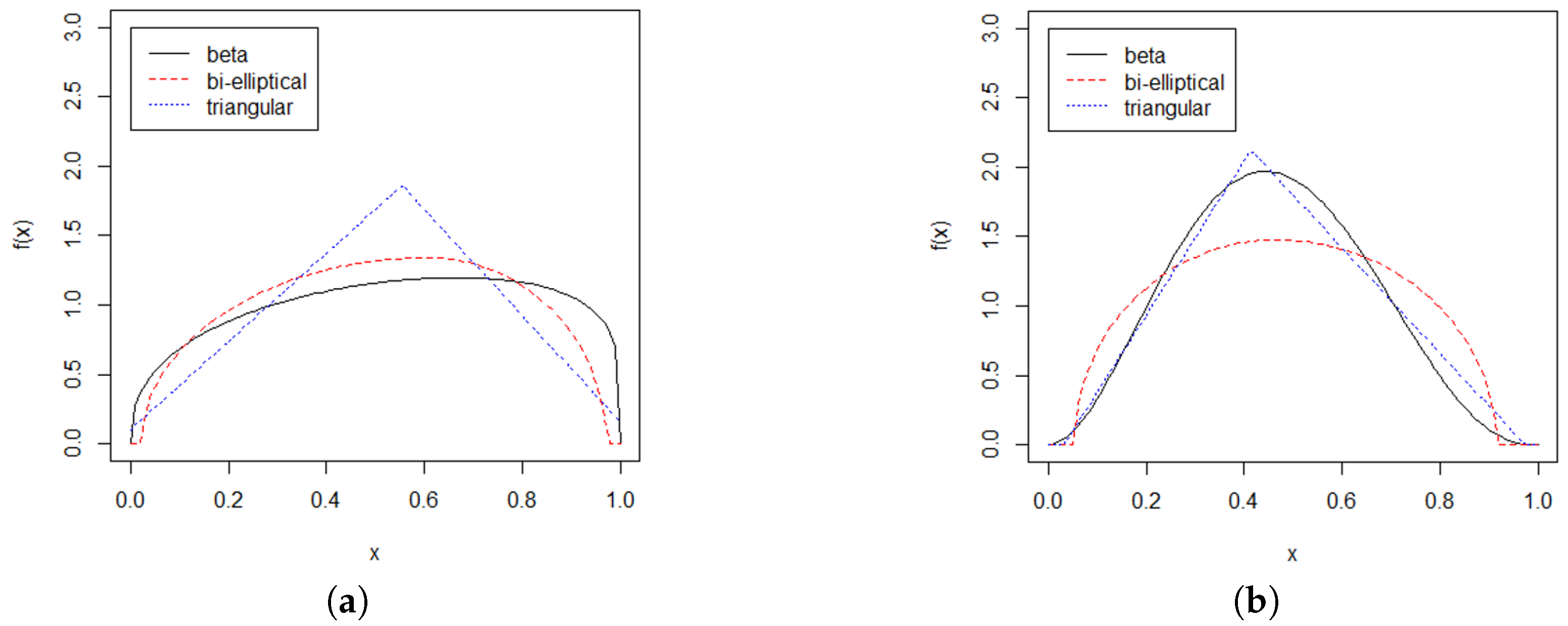
5. Comparing the Bi-Elliptic Distribution and the Triangular Distribution as a Proxy for the Beta Distribution

In the literature, one application of the triangular distribution is to serve as a proxy for the beta distribution. Ref. [11] noted that “the differences between the two distribution functions are seldom significant”. In this section, we present empirical results comparing the bi-elliptic distribution and the triangular distribution as a proxy for the beta distribution. We consider 81 beta distributions resulting from combinations of nine different values of the two shape parameters $\alpha$ and $\beta$. For each selected beta distribution, we draw 1000 samples of size 100, fit the data with the bi-elliptic distribution and the triangular distribution. Based on the MLE estimates, we compute the corresponding AICs and the Akaike weights of the two models. To obtain the Akaike weights, we first compute, for each model, the differences in AIC with respect to the AIC of the best candidate model [23]:

$${\Delta }_i\left(AIC\right)=AI{C}_i-min\left(AIC\right),$$

(32)

where i is either “bi-elliptic” or “triangular”. Then, the Akaike weights are computed:

$$w_i\left(AIC\right)={\displaystyle \frac{exp\{-\frac{1}{2}{\Delta }_i\left(AIC\right)\}}{\sum exp\{-\frac{1}{2}{\Delta }_k\left(AIC\right)\}}}.$$

(33)

Weight $w_i\left(AIC\right)$ can be interpreted as the probability that $M_i$ is the best model (in the AIC sense that it minimizes the Kullback–Leibler discrepancy), given the data and the set of candidate models [23].

To compare the bi-elliptic model and the triangular model, we compute the ratio

$$r={\displaystyle \frac{w_{bi-elliptic}}{w_{bi-elliptic}+w_{triangular}}},$$

(34)

which gives the normalized probability that the bi-elliptic model is to be preferred over the triangular model.

Table 4. Comparing the bi-elliptic and triangular distribution as a proxy for the beta distribution.

	$\mathit{\alpha }$	1	1.2	1.4	1.6	1.8	2	2.5	3	3.5
$\beta =1$	$AI{C}_{be}$	10.066	1.918	−6.733	−14.623	−22.296	−29.908	−45.229	−61.163	−74.815
	$AI{C}_t$	23.765	13.193	0.262	−11.879	−23.828	−35.026	−57.999	−79.103	−96.519
	%	99%	99%	92%	68%	39%	20%	4%	0.70%	0.50%
	r	99%	97%	87%	65%	41%	23%	5%	2%	0.90%
$\beta =1.2$	$AI{C}_{be}$	6.173	3.081	−2.514	−10.034	−16.564	−23.794	−39.446	−54.045	−67.704
	$AI{C}_t$	17.767	14.166	7.386	−3.13	−12.592	−22.43	−44.675	−64.882	−82.487
	%	95%	96%	99%	91%	77%	61%	22%	8%	4%
	r	94%	97%	96%	87%	73%	58%	24%	9%	4%
$\beta =1.4$	$AI{C}_{be}$	−1.700	−1.610	−3.815	−8.597	−14.277	−19.959	−34.647	−48.833	−62.024
	$AI{C}_t$	4.162	7.042	4.775	−1.359	−8.858	−16.679	−36.352	−54.951	−71.696
	%	84%	96%	97%	94%	85%	72%	38%	18%	10%
	r	81%	93%	93%	90%	81%	70%	40%	21%	12%
$\beta =1.6$	$AI{C}_{be}$	−8.647	−7.736	−8.192	−10.410	−14.568	−19.127	−31.892	−44.586	−57.418
	$AI{C}_t$	−6.283	−2.150	−1.422	−4.286	−9.734	−15.477	−32.175	−48.420	−64.392
	%	66%	88%	93%	91%	86%	78%	49%	28%	16%
	r	62%	82%	88%	86%	80%	73%	49%	30%	19%
$\beta =1.8$	$AI{C}_{be}$	−17.017	−14.320	−13.379	−14.247	−16.075	−20.384	−30.409	−42.249	−53.422
	$AI{C}_t$	−18.339	−11.950	−8.839	−9.589	−11.858	−17.318	−30.354	−44.83	−58.678
	%	40%	70%	82%	85%	82%	74%	50%	33%	21%
	r	42%	67%	78%	79%	77%	70%	50%	36%	24%
$\beta =2$	$AI{C}_{be}$	−24.240	−21.475	−19.367	−18.221	−20.012	−22.113	−31.092	−41.352	−51.936
	$AI{C}_t$	−27.151	−21.733	−16.687	−14.860	−17.067	−19.831	−30.899	−43.639	−56.88
	%	24%	52%	71%	77%	72%	68%	53%	35%	21%
	r	28%	51%	67%	73%	69%	65%	52%	37%	25%
$\beta =3$	$AI{C}_{be}$	−61.550	−53.756	−47.594	−44.105	−41.357	−40.748	−42.803	−47.288	−53.401
	$AI{C}_t$	−76.637	−65.648	−55.050	−48.96	−45.003	−43.972	−45.472	−50.903	−58.258
	%	6%	7%	14%	22%	26%	31%	30%	25%	21%
	r	7%	9%	17%	25%	31%	32%	34%	29%	24%
$\beta =3.5$	$AI{C}_{be}$	−75.059	−68.325	−60.512	−55.512	−53.495	−50.528	−50.604	−53.617	−57.843
	$AI{C}_t$	−88.337	−84.029	−72.241	−64.083	−60.338	−56.246	−55.619	−58.229	−63.477
	%	1.50%	4%	7%	13%	14%	20%	22%	22%	20%
	r	1.50%	6%	10%	15%	17%	22%	25%	25%	22%
$\beta =4$	$AI{C}_{be}$	−89.653	−82.796	−72.130	−67.252	−63.540	−60.938	−59.210	−60.364	−62.992
	$AI{C}_t$	−114.394	−101.53	−88.022	−78.783	−72.639	−68.977	−65.661	−66.351	−69.603
	%	0.20%	6%	5%	8%	10%	12%	17%	17%	15%
	r	0.70%	7%	6%	10%	12%	16%	19%	20%	18%

reports the mean AIC, the percentage of times that the AIC value corresponding to the bi-elliptic distribution ($AI{C}_{be}$) is smaller than that of the triangular distribution ($AI{C}_t$) in 1000 simulations, and the ratio r for different combinations of the shape parameters $\alpha$ and $\beta$. Compared to triangular distributions, bi-elliptic distributions offer a significantly better proxy for the beta distributions with different combinations of $\alpha$ and $\beta$ between 1 and 2. For instance, when $\alpha =1$, there is a probability between 81% and 99% that the bi-elliptic proxy is superior compared to the triangular proxy for $\beta$ between 1 and 1.4. As $\alpha$ increases, the range for “acceptable” $\beta$ (in terms of providing a high probability r of at least 70%) broadens, but never exceeds $\beta =2$. Due to the mirror-image symmetry of the beta densities, similar behavior of the probability r can be observed when $\beta$ is fixed and $\alpha$ varies. Figure 3a shows the density of the beta distribution with $\alpha =1.4$ and $\beta =1.2$ with the fitted curves using the bi-elliptical distribution and the triangular distribution. When the beta density resembles the bi-elliptical distribution, the later proves to be a much better proxy compared to the triangular distribution.

On the other hand, when either $\alpha$ or $\beta$ is greater than 2, the triangular distribution appears to be a better proxy for the beta distribution. For example, when $\beta =1$, there is a probability between 0.5% and 20% that the bi-elliptic proxy is superior compared to the triangular proxy for $\alpha$ between 2 and 3.5. Or equivalently, there is a probability between 80% and 99.5% that the triangular proxy is more preferable to the bi-elliptic one for $\alpha$ between 2 and 3.5 and $\beta =1$. As seen in Figure 3b, where the beta density with $\alpha =3$ and $\beta =3.5$ plotted together with the bi-elliptical and triangular fits, the triangular fit appears to be a better fit.

6. Conclusions

In this paper, we proposed a new family of bi-elliptic distributions supported on a bounded interval, constructed from elliptical arcs. We analyzed their theoretical properties, including the probability density function, cumulative distribution function, and moments, and compared their behavior to well-known bounded distributions such as the beta and triangular distributions. Simulation results show that in certain parameter settings, the bi-elliptic distributions can serve as a more flexible or accurate proxy to beta distributions than the triangular alternative.

While our results demonstrate the theoretical advantages of the proposed distributions, we did not claim universal superiority over existing distributions across all practical settings. One potential limitation of this study is the absence of a real-world application. We chose to omit such a case study in this initial work to maintain a clear focus on the theoretical framework. Moreover, application to a specific dataset may introduce domain-dependent assumptions and confounding factors, which could obscure the generality of the distribution’s utility.

As part of future research, we plan to explore applications of the bi-elliptic distribution in real-world contexts, such as risk analysis or reliability engineering. This will enable us to further validate its practical relevance and provide comparative performance analysis with triangular and beta distributions in applied settings.

References

1. Kotz, S.; van Dorp, J.R. Beyond Beta: Other Continuous Families of Distributions with Bounded Support and Applications; World Scientific: Singapore, 2004. [Google Scholar]
2. García, C.B.; García Pérez, J.; van Dorp, J.R. Modeling heavy-tailed, skewed and peaked uncertainty phenomena with bounded support. Stat. Methods Appl. 2011, 20, 463–486. [Google Scholar] [CrossRef]
3. Condino, F.; Domma, F. A new distribution function with bounded support: The reflected generalized Topp-Leone power series distribution. Metron 2017, 75, 51–68. [Google Scholar] [CrossRef]
4. Mazucheli, J.; Menezes, A.F.; Dey, S. Unit-Gompertz distribution with applications. Statistica 2019, 79, 25–43. [Google Scholar]
5. Ghitany, M.E.; Mazucheli, J.; Menezes, A.F.B.; Alqallaf, F. The unit-inverse Gaussian distribution: A new alternative to two-parameter distributions on the unit interval. Commun. Stat. Theory Methods 2018, 48, 3423–3438. [Google Scholar] [CrossRef]
6. Bakouch, H.S.; Nik, A.S.; Asgharzadeh, A.; Salinas, H.S. A flexible probability model for proportion data: Unit-half-normal distribution. Commun. Stat. Case Stud. Data Anal. Appl. 2021, 7, 271–288. [Google Scholar] [CrossRef]
7. Gemeay, A.M.; Sapkota, P.L.; Tashkandy, Y.A.; Bark, M.E.; Balogun, O.S.; Hussam, E. New bounded probability model: Properties, estimation, and applications. Heliyon 2024, 10, e38965. [Google Scholar] [CrossRef] [PubMed]
8. Goel, N.S.; Strebel, D.E. Simple beta distribution representation of leaf orientation in vegetation canopies. Agron. J. 1984, 76, 800–802. [Google Scholar] [CrossRef]
9. McDonald, J.B.; Xu, Y.J. A generalization of the beta distribution with applications. J. Econom. 1995, 66, 133–152. [Google Scholar] [CrossRef]
10. Gupta, A.K.; Nadarajah, S. Handbook of Beta Distribution and Its Applications; CRC Press: Boca Raton, FL, USA, 2004. [Google Scholar]
11. Johnson, D. The triangular distribution as a proxy for the beta distribution in risk analysis. J. R. Stat. Soc. Ser. D 1997, 46, 387–398. [Google Scholar] [CrossRef]
12. Dorp, J.; Kotz, S. Generalized trapezoidal distributions. Metrika 2003, 58, 85–97. [Google Scholar] [CrossRef]
13. Dorp, J.; Kotz, S. A novel extension of the triangular distribution and its parameter estimation. J. R. Stat. Soc. Ser. D 2002, 51, 63–79. [Google Scholar]
14. Karlis, D.; Xekalaki, E. The Polygonal Distribution. In Advances in Mathematical and Statistical Modeling in Honor of Enrique Castillo; Arnold, B.C., Balakrishnan, N., Minués, M., Sarabia, J.M., Eds.; Birkhäuser: Boston, MA, USA, 2008; pp. 21–33. [Google Scholar]
15. Vander Wielen, M.; Vander Wielen, R. The general segmented distribution. Commun. Stat. Theory Methods 2015, 44, 1994–2009. [Google Scholar] [CrossRef]
16. Mazucheli, J.; Menezes, A.F.B.; Dey, S. The unit-Birnbaum-Saunders distribution with applications. Chil. J. Stat. 2018, 9, 47–57. [Google Scholar]
17. Coad, A. The Growth of Firms: A Survey of Theories and Empirical Evidence; Edward Elgar Publishing Ltd.: Cheltenham, UK, 2009. [Google Scholar]
18. Mulligan, D.W. Improved Modeling of Three-Point Estimates for Decision Making: Going Beyond the Triangle; Naval Postgraduate School: Monterey, CA, USA, 2016. [Google Scholar]
19. Fletcher, S.G.; Ponnambalam, K. Stochastic control of reservoir systems using indicator functions: New enhancements. Water Resour. Res. 2008, 44. [Google Scholar] [CrossRef]
20. Brent, R.P. An algorithm with guaranteed convergence for finding a zero of a function. Comput. J. 1971, 14, 422–425. [Google Scholar] [CrossRef]
21. Lange, K. MM Optimization Algorithms; Society for Industrial and Applied Mathematics: Philadelphia, PA, USA, 2016. [Google Scholar]
22. Byrd, R.H.; Lu, P.; Nocedal, J.; Zhu, C. A limited memory algorithm for bound constrained optimization. SIAM J. Sci. Comput. 1995, 16, 1190–1208. [Google Scholar] [CrossRef]
23. Burnman, K.P.; Anderson, D.R. Model Selection and Multimodel Inference, A Practical Information-Theoretic Approach; Springer: New York, NY, USA, 2002. [Google Scholar]
Figure 1. PDF and CDF of E ( 0 , 1 , m ) distributions for different choices of m: m = 0.1 , 0.3 , 0.5 , 0.7 , 0.9 .
Mathematics 13 01811 g001
Figure 2. Survival and hazard functions of E ( 0 , 1 , m ) distributions for different choices of m: m = 0.1 , 0.3 , 0.5 , 0.7 , 0.9 .
Mathematics 13 01811 g002
Figure 3. Density plots of true beta distribution with the bi-elliptical fit and triangular fit: (a) α = 1.4 , β = 1.2 and (b) α = 3 ,   β = 3.5 .
Mathematics 13 01811 g003