Mixed-Order Fuzzy Time Series Forecast

Abstract

Fuzzy time series forecasting has gained significant attention for its accuracy, robustness, and interpretability, making it widely applicable in practical prediction tasks. In classical fuzzy time series models, the lag order plays a crucial role, with variations in order often leading to markedly different forecasting results. To obtain the best performance, we propose a mixed-order fuzzy time series model, which incorporates fuzzy logical relationships (FLRs) of different orders into its rule system. This approach mitigates the uncertainty in fuzzy forecasting caused by empty FLRs and FLR groups while fully exploiting the fitting advantages of different-order FLRs. Theoretical analysis is provided to establish the mathematical foundation of the mixed-order model, and its superiority over fixed-order models is demonstrated. Simulation studies reveal that the proposed model outperforms several classical time series models in specific scenarios. Furthermore, applications to real-world datasets, including a COVID-19 case study and a TAIEX financial dataset, validate the effectiveness and applicability of the proposed methodology.

1. Introduction

It is well known that fuzzy sets are somewhat like sets whose elements have degrees of membership. Since Lotfi A. Zadeh [1] introduced the concept of a fuzzy set as an extension of the classical notion of a set, it has been established as an important and practical modeling tool. For time series analysis, Song and Chissom [2,3,4] first transformed the observed time series to a fuzzy time series (FTS) and built FLRs for forecasting. Now, FTS forecasting is not only an extension of the time series approach applied to fuzzy sets but also a representative combination of intelligent algorithms and econometric methods [5,6,7,8,9,10,11]. Although FTS forecasting is a multidisciplinary approach, its core primarily involves the identification of FLRs and forecasting [12,13,14]. The process consists of three fundamental steps: fuzzification, identification of FLRs, and defuzzification.

In the fuzzification step, how to determine the length of the interval is a key issue. Relevant research in this direction can be divided into three categories. The first one is to take the length as a statistic parameter, including the data range [2,3,4], the data average [15], and other distribution-based parameters [16]. The second category is to construct an optimization problem for obtaining the length of the fuzzy intervals. The minimization of mean squared errors (MSE) is the goal of this kind of research. The quadratic optimization algorithms [17,18], intelligent algorithms [19,20], and information entropy methods [21], among others, are often used to optimize interval segmentation. The third category is to use clustering methods to realize the division of the variable universe, which includes Gath–Geva clustering [22], automatic clustering [23], affinity propagation clustering [24], etc. For illustration, in this paper we employ fuzzy c-means (FCM) clustering [25] to produce the interval segmentation, even though others are applicable. This method can effectively describe the memberships of data and form interpretable fuzzy intervals.

In the step of the identification of FLRs, a fixed-order [15,16,17] or high-order FLR [26,27] is employed. Typically, one chooses an optimal fixed-order FLR model to minimize the MSE [21,28,29]. There are also other attempts; for example, Ye et al. [30] used the weighted values of predictions from first-, second-, and third-order models. However, there still exist unsatisfactorily fitting segments in the application of different-order models. Naturally, one asks whether or not different-order FLRs can be combined for a better forecast. This motivates us to propose a mixed-order FLR model, which integrates different-order FLRs. The model seeks to find a unique best-matching FLR in the rule base, which avoids the confusion caused by FLR groups (FLRGs) and empty FLRs. To demonstrate the advantages of our method, we not only prove some of its properties but also compare it with classic ones in the literature [31,32,33,34,35,36]. Theoretically and practically, we show that the performance of the mixed-order FLRs is better than the fixed-order ones.

In the defuzzification step, one needs to transform the predicted fuzzy sets into the most representative real number. Usually, the center of the observations is used as a representative of the predicted fuzzy set [6,7,37]. Despite the intention of mixed-order FLRs to mitigate confusion stemming from FLRGs and empty FLRs, situations may still arise where empty FLRs and FLRGs unavoidably occur. For the completeness of the defuzzification rules, the classical methods, including the master voting scheme [20] and the mean method, are used to defuzzify the fuzzy set from empty FLRs and FLRGs.

Applying the above three steps, we obtain an FTS forecast procedure built upon a mixed-order FLR model. In practice, for a given sample, one needs to specify the order of the model as in classic time series analysis. We develop the well-known K-fold cross-validation criterion [38,39,40] to select the best mixed-order models for the sample. This furnishes us a data-driven FTS forecast approach.

To theoretically demonstrate the superiority of the mixed-order model over fixed-order models, we define the completeness and redundancy to characterize the set of empty FLRs and FLR groups, respectively. To explore the predictive relationships among different-order models, we introduce the sub-FLR and extended FLR to describe the relationships between FLRs with different orders that share the same components. Several favorable properties of the mixed-order model are identified: the first-order model has the greatest probability of generating a complete FLR set among all orders, and high-order redundant sets can always be derived from low-order redundant sets. To further validate the effectiveness of the mixed-order model, we conduct comparisons with other models using both synthetic and real-world datasets, providing additional insights into the applicability of the mixed-order model.

The remainder of this paper is organized as follows. In Section 2, we give a brief review of FTS, introduce the mixed-order FLRs, and develop the related mathematical theory. In Section 3, we introduce our FTS forecast method and the corresponding algorithm. In Section 4, we conduct numerical experiments to compare different methods. Finally, we conclude this paper. All proofs of theorems are postponed to the Appendix A.

2. FTS and Mixed-Order FLR Models

To motivate our mixed-order FLR models, let us first review the FTS.

2.1. Review of Fuzzy Time Series

For convenience of exposition, let us first introduce some definitions.

Definition 1

(Fuzzy Set [1]). Let the universe of discourse be $U=\left\{u_1,u_2,\dots ,u_n\right\}$, and a fuzzy set A of U is characterized by a membership function ${\mu }_A:U\to [0,1]$, expressed as

$$A={\mu }_A\left(u_1\right)/u_1+{\mu }_A\left(u_2\right)/u_2+\dots +{\mu }_A\left(u_n\right)/u_n$$

(1)

where ${\mu }_A\left(u_i\right)\in [0,1]$ represents the grade of membership of $u_i$ in A, the symbol “/” separates the membership grades from the elements in U, and the symbol “+” means “union” rather than the algebraic symbol of summation.

Definition 2

(FTS [3]). Let $X\left(t\right),t=\dots ,0,1,2,\dots$, a subset of $\mathbb{R}$, be the universe of discourse in which fuzzy sets $f_i\left(t\right)$, $i=1,2,\dots$, are defined, and $F\left(t\right)$ is the collection of $f_i\left(t\right)$, $i=1,2,\dots$. Then, $F\left(t\right)$ is called a fuzzy time series on $X\left(t\right),t=\dots ,0,1,2,\dots$.

Here, $F\left(t\right)$ can be viewed as a linguistic variable, and $f_i\left(t\right)$ can be regarded as possible linguistic values of $F\left(t\right)$. If the maximum degree of membership of $F(t-i)$ belongs to fuzzy set $A_{t_i}$, $i=0,\dots ,m$, then the m-order FLR between $F(t-m),\dots ,F(t-1)$ and $F\left(t\right)$ can be represented as

$$A_{t_m},\dots ,A_{t_1}\to A_{t_0}.$$

(2)

FLRs with the same left-hand side can be grouped together and are called an FLR group.

On one hand, it is worth noting that using the collection of all FLRs based on the fuzzy sample is not enough for fuzzy forecasting in all possible situations, since there may not exist a forecast. In general, if there is no fuzzy forecast based on a fuzzy set series “$A_{i_m},\dots ,A_{i_1}$”, then we use

$$A_{i_m},\dots ,A_{i_1}\to \#$$

(3)

to denote such an FLR. We call it an empty m-order FLR. That is, the one-step fuzzy forecast based on $A_{i_m},\dots ,A_{i_1}$ is not available.

On the other hand, if there is an m-order FLRG, then there are multiple fuzzy forecasts, and thus it is confusing to determine which to choose for the forecast. This motivates us to introduce the mixed-order FLRs to solve these problems.

2.2. Mixed-Order FLRs

To develop the mixed-order FLRs, we first define complete FLR sets and redundant FLR sets. The ideas of completeness and redundancy are similar to those of the rule-based system [41].

Definition 3

(Completeness). A set of m-order FLRs is complete if there is no empty m-order FLR in the set; otherwise, it is incomplete.

Definition 4

(Redundancy). A set of m-order FLRs is non-redundant if it contains no m-order FLRG; otherwise, it is redundant.

Let A be an FTS, $F_m\left(A\right)$ be the set consisting of all m-order FLRs derived from A, $E_m\left(A\right)$ be the incomplete FLR set composed of all empty m-order FLRs, and $R_m\left(A\right)$ be the redundant complete FLR set composed of all m-order FLRGs. Let $C_m\left(A\right)=F_m\left(A\right)\setminus (E_m\left(A\right)\cup R_m\left(A\right)),$ that is, $C_m\left(A\right)$ is a complete and non-redundant FLR set composed of m-order FLRs which are not empty and not in any FLRGs. Then, for a given m, we have

$$F_m\left(A\right)=E_m\left(A\right)\cup C_m\left(A\right)\cup R_m\left(A\right)$$

(4)

Due to the randomness of A, the FLR set $F_m\left(A\right)$ is random, and thus $E_m\left(A\right)$, $C_m\left(A\right)$ and $R_m\left(A\right)$ are, too. $F_m\left(A\right),E_m\left(A\right),R_m\left(A\right)$ and $C_m\left(A\right)$ are abbreviated as $F_m,E_m,R_m$ and $C_m$. If $E_m$ and $R_m$ are empty sets, then $F_m=C_m$, which is an ideal case and does not hold in general.

Our idea for the mixed-order FLR model is to construct as close to a one-to-one relationship between the left-hand fuzzy series and the right-hand fuzzy set as possible. Ideally, if the m-order model ($F_m$) is used for prediction, we hope it is complete and non-redundant, because a fuzzy forecast cannot be obtained from the empty FLR in $E_m$ and is confronted with multiple predictions from the FLRGs in $R_m$. Our mixed-order model attempts to achieve this goal. To this end, we begin with a simple set which has the greatest probability of being a complete FLR set, and then shrink the redundancy step by step. The following theorem suggests that $F_1$ is the desired set with which we should start.

Theorem 1.

For every FTS, $F_1$ has the greatest probability of being a complete FLR set among all $F_m$, $m=1,2,\dots$.

According to Theorem 1, we begin with $F_1=E_1\cup C_1\cup R_1$ for constructing the mixed-order FLRs. Since $E_1$ (as well as $E_k$, $k>1$) cannot provide any information for forecasting the next state, if $R_1$ is empty, then $F_1$ is a desired model for the fuzzy forecast. Otherwise, we need to deal with $R_1$, which is complete but redundant. To this end, we introduce the concepts of “sub-FLR” and “extended-FLR” in the following.

Definition 5

(Sub-FLR/Extended FLR). Given a j-order FLR

$$A_{k_j}{A}_{k_{j-1}}\dots A_{k_{i+1}}{A}_{k_i}\dots A_{k_1}\to A_{k_0},$$

(5)

for $i\le j$, the i-order FLR $\{A_{k_i}\dots A_{k_1}\to A_{k_0}\}$ is called the sub-FLR of the FLR (5), and, conversely, the FLR (5) is called the extended FLR of the i-order FLR.

Obviously, a sub-FLR shares the same one-step fuzzy forecast with the original FLR. For any i-order FLR set $B_i\subseteq F_i$ and $(i+1)$-order FLR set $D_{i+1}\subseteq F_{i+1}$, we define

$$D_{i+1}\left(B_i\right)=\{T_{i+1}:\begin{array}{c}{T}_{i+1}\in D_{i+1}\mathrm{and}\mathrm{there}\mathrm{exists}\mathrm{a}{T}_i\in B_i\\ \mathrm{such}\mathrm{that}{T}_{i+1}\mathrm{is}\mathrm{an}\mathrm{extended}\mathrm{FLR}\mathrm{of}{T}_i\end{array}\}.$$

(6)

The redundancy of $F_1$ (or $R_1$) can be shrunk by replacing all first-order FLRGs in $R_1$ with their extended FLRs. Based on the Occam’s razor principle, it is natural to extend them to the second-order FLRs, which are simplest among all higher-order FLRs. Hence, we replace $R_1$ with $F_2\left(R_1\right)$. By Equation (4), we have

$$F_2\left(R_1\right)=E_2\left(R_1\right)\cup C_2\left(R_1\right)\cup R_2\left(R_1\right).$$

(7)

It is obvious that $R_2\left(R_1\right)=R_2$. More generally, we have the following result.

Theorem 2.

$R_{m+1}\left(R_m\right)=R_{m+1}$.

Because each element in $E_2$ is an empty FLR, and each element in $R_1$ is a nonempty FLR, $E_2\left(R_1\right)=\varphi$. By Theorem 2, Equation (7) becomes

$$F_2\left(R_1\right)=C_2\left(R_1\right)\cup R_2.$$

(8)

In general, similarly to Equation (8),

$$F_{k+1}\left(R_k\right)=C_{k+1}\left(R_k\right)\cup R_{k+1},\mathrm{for}k\ge 1,$$

(9)

where $C_{k+1}\left(R_k\right)$ is a non-redundant and complete subset of $C_{k+1}$. Then, the first-order FLR set $F_1$ can be replaced by a mixed-order FLR set

$$M_2=E_1\cup C_1\cup C_2\left(R_1\right)\cup R_2.$$

(10)

If $R_2$ is empty, then model $M_2$ is desired. Otherwise, we replace $R_2$ with $F_3\left(R_2\right)$ and obtain the model

$$M_3=E_1\cup C_1\cup \left[{\cup }_{k=2}^3{C}_k\left(R_{k-1}\right)\right]\cup R_3.$$

(11)

After repeating the process of replacing $R_k$ with $F_{k+1}\left(R_k\right)$ up to $k=m_{max}-1$ ($m_{max}$ is the maximum lag order allowed by the method), we obtain a sequence of FLR models:

$$M_m=E_1\cup C_1\cup \left[{\cup }_{k=2}^m{C}_k\left(R_{k-1}\right)\right]\cup R_m,m=2,\dots ,m_{max},$$

(12)

and $M_1$ is defined as $F_1$. Since each $M_m$ consists of different-order FLRs, we call it the mth mixed-order FLR model. As m gets larger, the model becomes more complicated. The parameter m can be regarded as a tuning parameter. Given a sample path, it can be chosen to minimize the mean squared errors in the forecast by K-fold cross-validation [39]. See Section 3.2 for detail.

Each of the mixed-order FLR models in Equation (12) consists of three parts: an incomplete subset $E_1$, complete non-redundant subset $C_1\cup \left[{\cup }_{k=2}^m{C}_k\left(R_{k-1}\right)\right]$, and redundant subset $R_m$. For the fixed-order model $F_m$ in Equation (4), the corresponding three parts are $E_m$, $C_m$, and $R_m$, respectively. Now, we compare $F_m$ with $M_m$. First, both of them have the same common part $R_m$. Given a sample path, as m gets large enough, $R_m$ will eventually be an empty set. (In an extreme case, for an FTS with $m+1$ observations, only one m-order FLR can be extracted, and $R_m=\varphi$). Second, by Theorem 1,

$$P(E_1=\varphi )\le P(E_m=\varphi ),\mathrm{for}\mathrm{any}\mathrm{given}m>1,$$

(13)

that is, the probability of an empty FLR appearing in $M_m$, $P(E_1=\varphi )$ is less than the probability of an empty FLR appearing in $F_m$, $P(E_m=\varphi )$. Third, for any FLR in $C_m$, there is a sub-FLR of $C_m$ in $C_1\cup \left({\cup }_{k=2}^m{C}_k\left(R_{k-1}\right)\right)$, as demonstrated in the following theorem.

Theorem 3.

For every m-order FLR in $C_m$, there exists a corresponding sub-FLR in $C_1\cup \left[{\cup }_{k=2}^m{C}_k\left(R_{k-1}\right)\right]$.

By Theorem 3, the corresponding fuzzy forecasts (right-hand side of FLR) in $C_m$ and $C_1\cup \left({\cup }_{k=2}^m{C}_k\left(R_{k-1}\right)\right)$ are the same because any sub-FLR shares the same one-step fuzzy forecast with the original FLR. Further, the FLR models in $C_1\cup \left({\cup }_{k=2}^m{C}_k\left(R_{k-1}\right)\right)$ are simpler than in $C_m$ due to the lower orders. Therefore, compared with the m-order FLR model $F_m$, the proposed model $M_m$ has the following advantages:

(i)

If $F_m$ has a nonempty prediction, $M_m$ has the same prediction, but not vice versa;

(ii)

$F_m$ has more empty predictions than $M_m$ because of Equation (13);

(iii)

$M_m$ is simpler than $F_m$ because of the lower FLR orders.

3. The Proposed FTS Forecast

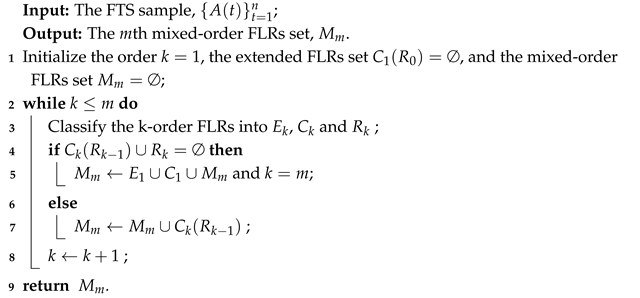
3.1. FTS Forecast Based on an mth Mixed-Order FLR

A traditional FTS forecasting method consists of fuzzification, FLR modeling, and defuzzification. In the following, we illustrate the proposed method in detail.

Step 1: Fuzzification. The aim of fuzzification is to assign each observation to a fuzzy set. It is similar to the clustering process. Given a training set $X=\{x_1,x_2,\dots ,x_n\}$, suppose we assign it into c fuzzy sets, $\{A_i,i=1,2,\dots ,c\}$. Let $u_{ij}$ be the degree of membership of $x_j$ assigned to fuzzy set $A_i$. The value of $u_{ij}$ is to be determined. Use the weighted average of training samples, $y_i={\sum }_{j=1}^n{\left(u_{ij}\right)}^k{x}_j/{\sum }_{j=1}^n{\left(u_{ij}\right)}^k$, to estimate the center of $A_i$, where k is the degree of fuzziness. (In this paper, the degree of fuzziness is set to 2, which is the same as [42]). Let $d(x_j,y_i)$ be the distance between $x_j$ and $y_i$. Denote with U a $c\times n$ fuzzy partition matrix with the $(i,j)$ component being $u_{ij}$. For clustering observations into c fuzzy sets, we employ the FCM algorithm [25], which produces an optimal c partition by minimizing the weighted within-group sum of squared error objective function

$$\begin{array}{ccc}& & g\left(U\right)=\sum _{i=1}^c\sum _{j=1}^n{\left(u_{ij}\right)}^k{d}^2(x_j,y_i)\hfill \end{array}$$

(14)

$$\begin{array}{ccc}\hfill s.t.& & y_i={\displaystyle \frac{{\sum }_{j=1}^n{\left(u_{ij}\right)}^k{x}_j}{{\sum }_{j=1}^n{\left(u_{ij}\right)}^k}},i=1,2,\dots ,c,\hfill \end{array}$$

(15)

$$\begin{array}{ccc}& & \sum _{i=1}^c{u}_{ij}=1,j=1,2,\dots ,n,\hfill \end{array}$$

(16)

$$\begin{array}{ccc}& & u_{ij}\ge 0,i=1,2,\dots ,c,j=1,2,\dots ,n.\hfill \end{array}$$

(17)

The above problem can be solved via iterations. When $\{y_1,\dots ,y_c\}$ are given, using the Lagrange multiplier method, one obtains the minimizer of $g\left(U\right)$ [25]:

$$u_{ij}={\left\{\sum _{r=1}^c{\left[{\displaystyle \frac{d(x_j,y_i)}{d(x_j,y_r)}}\right]}^{{\displaystyle \frac{2}{k-1}}}\right\}}^{-1},1\le i\le c,1\le j\le n.$$

(18)

Then, update the values of $y_i$ in Equation (15). Repeat this procedure until convergence. Then, one gets the optimal solution of U and assigns $x_j$ to fuzzy set $A_i$ if $u_{ij}=max\left\{u_{lj},l=1,2,\dots ,c\right\}$. The fuzzy sets $A_i$ can be set as, for example,

$$A_i=(b_{i-1},b_i],$$

where $b_0=mi{n}_j\left\{x_j\right|x_j\in X\}-\Delta$, $b_i$ is the maximum value of $x_j$’s which are assigned to $A_i$, and $\Delta$ can be any small number as long as $b_0<min\left\{x_j\right|x_j\in X\}$ [43].

Step 2: Identification of mixed-order FLRs

According to Section 2.2, a key process of the mth mixed-order FLRs in Equation (12) is to replace $R_k$ with $C_{k+1}\left(R_k\right)\cup R_{k+1}$ in Equation (9). The algorithm for constructing the mth mixed-order FLRs is shown in Algorithm 1.

Algorithm 1: Generation of the mth mixed-order FLRs

Step 3: Defuzzification

Defuzzification acts as a translator of the fuzzy system. It consists of two parts: selecting the FLR and defuzzifying the fuzzy forecasting result.

Suppose there is an FLR with “$A_{?}$” being the fuzzy forecast from $F_m$. By Theorem 3, there exists a sub-FLR of “$A_{t_m},\dots ,A_{t_1}\to A_{?}$” in $C_1\cup \left[{\cup }_{k=2}^m{C}_k\left(R_{k-1}\right)\right]\subseteq M_m$. The sub-FLR can be found by checking the FLR in $M_m$ from the first to the mth order, as illustrated in Algorithm 2. According to the property of sub-FLRs, a sub-FLR shares the same one-step fuzzy forecast with the original FLR, thus “$A_{?}$” can be determined.

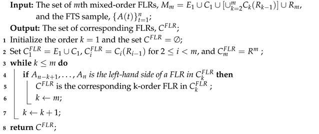
Algorithm 2: The FLR selection

Per the number of items in the one-step fuzzy forecast set, we define the following three defuzzified rules to select the representative of the predicted fuzzy set. The representative of the fuzzy set is defined as the center of the observations. Notice that, even if $M_m$ aims to establish one-to-one FLRs, empty FLRs and FLRGs may appear in the forecasting. Thus, the weighted average of the centers is used to represent the predicted fuzzy set from empty FLRs and FLRGs.

Case I.

If the one-step fuzzy forecast is a single fuzzy set, like $A_{i_m}\dots A_{i_1}\to A_j$, the defuzzified value $z_j$ of fuzzy set $A_j$ is defined as

$$z_j=arg\underset{z}{min}{n}_j^{-1}\sum _{j=1}^{n_j}{(z-x_j^{(i_m\dots i_{i_1})})}^2,$$

(19)

where $x_j^{(i_m\dots i_{i_1})}$ represents the observations corresponding to the next state $A_j$, which has a fuzzy logical relationship: $A_{i_m}\dots A_{i_1}\to A_j$, $n_j$ is the total number of observations whose next state is $A_j$. Hence, the solution to Equation (19) is $z_j=n_j^{-1}{\displaystyle \sum _{j=1}^{n_j}}{x}_j^{(i_m\dots i_{i_1})}$.

Case II.

If the one-step fuzzy forecast is an empty set, like $A_{i_m}\dots A_{i_1}\to \#$, the defuzzified value $z_{\#}$ is calculated by the master voting scheme [20]:

$$z_{\#}={\displaystyle \frac{m{c}_{i_1}+c_{i_2}+\dots +c_{i_m}}{2m-1}}.$$

(20)

where $c_{i_m}$ is the center value of the observations in fuzzy set $A_{i_m}$, $c_{i_m}=n_{i_m}^{-1}{\displaystyle \sum _{j=1}^{n_{i_m}}}{x}_j^{i_m}$. Since there is no nonempty FLR as the basis in this case, the left-hand side of the empty FLR is the only useful information in the prediction. The weighted average of the centers is employed, and the greatest weight m is given to the center of $A_{i_1}$ because $A_{i_1}$ is the most recent fuzzy set for the prediction.

Case III.

If the one-step fuzzy forecast is multiple fuzzy sets, like $A_{i_m}\dots A_{i_1}\to \{A_{j_1}\dots A_{j_l}\}$, the defuzzified value is the average of the forecasting fuzzy set.

$$z_{(j_1\dots j_l)}={\displaystyle \frac{c_{j_1}+\dots +c_{j_l}}{l}}.$$

(21)

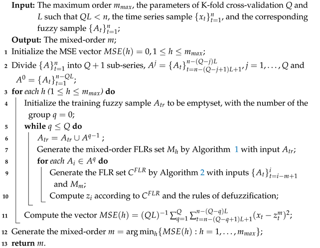
3.2. Choice of the Mixed-Order m

In Section 3.1, we need a predetermined value of m. The larger m is, the more complicated the model becomes. Hence, we regard it as a tuning parameter. Suppose there is a fuzzy time series sample of size n, ${\left\{A_t\right\}}_{t=1}^n$. We extend the K-fold cross-validation [39] to the current situation for the choice of m. The basic idea of this method is to choose m to minimize the prediction’s mean squared errors, and the details are given in Algorithm 3.

Algorithm 3: Selection of mixed-order m

4. Experimental Results

In this section, we demonstrate the effectiveness of the mixed-order model through numerical experiments on both synthetic and real-world datasets. First, we compare the mixed-order model with fixed-order models on eight different types of non-stationary time series to analyze the scenarios where the mixed-order model is more applicable. Subsequently, we apply both mixed-order and fixed-order models to real-world datasets to verify the superiority of the mixed-order model. Finally, we compare the mixed-order model with models proposed in other studies. All methods are implemented in MATLAB R2023b and executed on a laptop with an Intel Core i5.

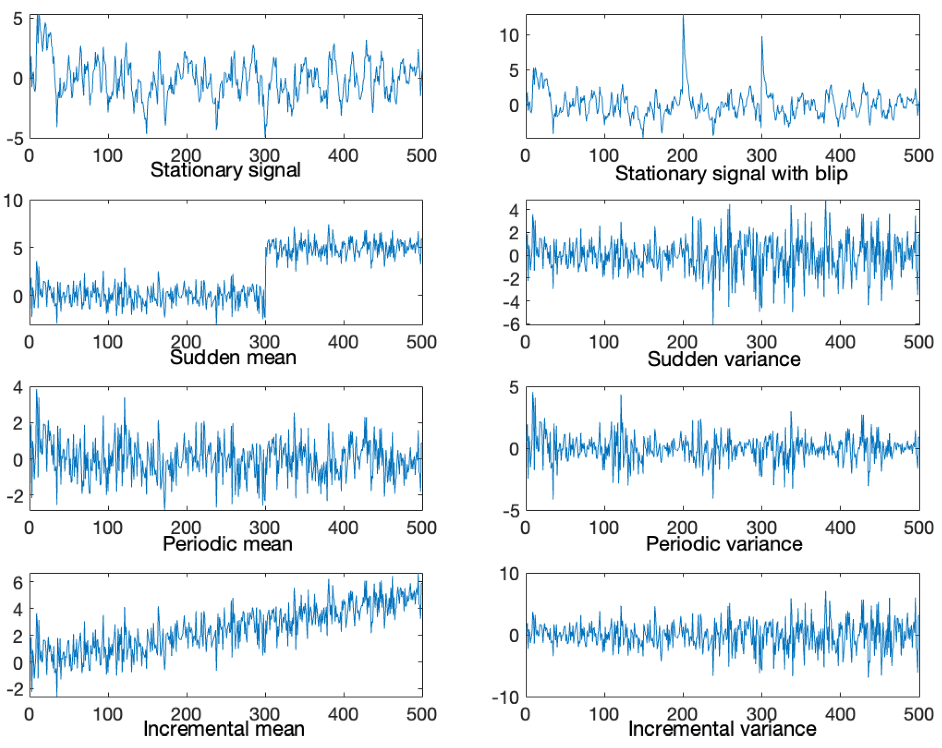
4.1. Performance Evaluation on Time Series Data with Varying Characteristics

To investigate the applicability of the mixed-order model, we conducted a comprehensive evaluation of its predictive performance on various synthetic time series with distinct characteristics. These time series include the following: stationary time series, stationary time series with blips, sudden changes in the mean and variance, periodic changes in the mean and variance, and incremental changes in the mean and variance. The dataset is visualized in Figure 1. To measure the forecast accuracy, we employ the square root of mean squared error (RMSE), which is defined as

$$\begin{array}{ccc}\hfill RMSE& =& {\left\{n^{-1}\sum _{t=1}^n{[\widehat{x}\left(t\right)-x\left(t\right)]}^2\right\}}^{1/2}.\hfill \end{array}$$

The comparative results of the RMSE among the mixed-order and fixed-order models are summarized in

Table 1. Comparison of mixed-order and fixed-order models for synthetic time series.

Model	Mixed-Order	1-Order	2-Order	3-Order	4-Order	5-Order
stationary	0.8235	0.8955	1.1270	1.0258	0.9462	0.9435
with blip	0.8211	0.8986	1.0879	1.0346	0.9465	0.9461
sud mean	0.9954	3.8836	2.8186	2.6188	2.6030	2.5867
sud var	1.6564	1.6575	1.9790	1.8039	1.7923	1.7938
per mean	0.8923	1.0137	1.1211	1.0262	0.9150	0.9150
per var	0.6403	0.6506	0.8664	0.6956	0.6769	0.6771
inc mean	0.9941	2.6994	2.7321	2.6395	2.5189	2.4948
inc var	2.8946	2.8045	3.0898	3.0272	3.0090	3.0166

.

The results clearly indicate that the mixed-order model consistently outperforms fixed-order models across all types of time series. Notably, the mixed-order model excels in handling non-stationary time series with periodic changes in variance, delivering superior performance even compared with its predictions on stationary time series. However, its weakest performance is observed on time series with incremental changes in variance, likely due to the growing number of unavoidable empty FLRs caused by the escalating variance in the data.

4.2. The Effectiveness of the Mixed-Order FLRs

Intuitively, the mixed-order model is an integration of multiple fixed-order models, which can easily produce a wide variety of FLRs. In order to demonstrate the effectiveness of the proposed mixed-order model, we compare it with different fixed-order models using the real-world dataset on the weekly percentage changes in newly confirmed COVID-19 cases published in the WHO Weekly Epidemiological Reports, as shown in Figure 2. (The sample used in this subsection consists of data from the first 100 COVID-19 Weekly Epidemiological Updates. The data are available on the official website of the WHO: https://www.who.int/emergencies/diseases/novel-coronavirus-2019/situation-reports/ accessed on 19 May 2025).

Based on the K-fold cross-validation in Algorithm 3 ($K=5$), we obtain $M_5$ as the mixed-order FLRs for fitting the data. The smaller the RMSEs are, the better the method becomes.

Table 2. Comparison between the mixed-order model and fixed-order models.

Model	Mixed-Order	1-Order	2-Order	3-Order	4-Order	5-Order
RMSE	0.1030	0.1789	0.1102	0.1215	0.1351	0.1393

reports the values of these measures, reflecting the nice performance of the mixed-order model. In fact, among the fixed-order models, the second-order model is the best, which indicates that the prediction accuracy is not always improved by merely increasing the order. As a whole, the mixed-order model has the smallest values of RMSE, which indicates that the mixed-order model is effective.

4.3. Comparison with Other Methods

For convenience of comparison, we use the TAIEX datasets from 2002 to 2004 (the data are available in Yahoo Finance: http://tradingeconomics.com/taiwan/stock-market/ accessed on 19 May 2025), which have been extensively analyzed in the the existing literature. The datasets are shown in Figure 3. In the experiment, the historical data of each year are divided into two parts: the historical data from January to October of each year are used as the training set, and the data from November to December of each year are the testing set.

Table 3. The comparison of the RMSEs for different methods.

No.	Methods	2002	2003	2004	Average RMSE
1	Huarng et al.’s method (Use NASDAQ) [31]	95.15	65.51	73.57	78.08
2	Huarng et al.’s method (Use Dow Jones) [31]	93.73	72.95	73.49	80.06
3	Huarng et al.’s method (Use M1b) [31]	97.10	75.23	82.01	84.78
4	Huarng et al.’s method (Use NASDAQ & Dow Jones) [31]	93.48	65.51	73.49	77.49
5	Huarng et al.’s method (Use NASDAQ & M1b) [31]	97.15	70.76	73.48	80.46
6	Huarng et al.’s method (Use NASDAQ & Dow Jones & M1b) [31]	95.73	70.76	72.35	79.61
7	The mixed-order method (with equal intervals and single variable)	80.68	55.67	76.54	70.96
8	AR (1) model [35]	97.09	91.67	79.94	89.57
9	AR (2) model [35]	89.80	66.58	60.33	72.24
10	Chen’s fuzzy time series model [32]	101.00	74.00	84.00	86.33
11	Univariate conventional regression model [33]	116.00	329.00	146.00	197.00
12	Univariate neural network-based fuzzy time series model [33]	84.00	56.00	116.00	85.33
13	The mixed-order method (univariate)	74.04	60.57	61.40	65.34
14	Bivariate conventional regression model [33]	77.00	54.00	85.00	72.00
15	Bivariate neural network-based fuzzy time series model [33]	85.00	58.00	67.00	70.00
16	Bivariate neural network-based fuzzy time series model use subsitutes [33]	80.00	58.00	67.00	68.33
17	Chen & Chang’s method (Use NASDAQ) [34]	73.06	66.36	60.48	66.63
18	Chen & Chang’s method (Use Dow Jones) [34]	79.81	64.08	82.32	75.40
19	Chen & Chang’s method (Use M1b) [34]	96.06	90.27	100.10	95.48
20	Chen & Chang’s method (Use NASDAQ & Dow Jones) [34]	72.33	60.29	68.07	66.90
21	Chen & Chang’s method (Use NASDAQ & M1b) [34]	76.48	53.51	69.29	66.43
22	Chen & Chen’s method (Use Dow Jones) [36]	74.65	66.02	58.89	66.52
23	Chen & Chen’s method (Use NASDAQ) [36]	71.01	65.14	61.94	66.03
24	Chen & Chen’s method (Use M1b) [36]	85.85	63.10	67.29	72.08
25	Chen & Chen’s method (Use M1b & Dow Jones) [36]	77.96	60.32	65.86	68.05
26	Chen & Chen’s method (Use M1b & NASDAQ) [36]	74.05	67.83	65.09	68.99
27	Chen & Chen’s method (Use NASDAQ & Dow Jones & M1b) [36]	77.38	60.65	65.09	67.71
28	LSTM-FTS method	89.00	92.00	70.00	84.00
29	NN-FTS method	80.00	58.00	67.00	68.00
30	The mixed-order method (use opening price)	73.14	57.93	56.38	62.48

shows a comparison of RMSEs and the average RMSEs.

The fuzzy intervals of Methods 1 and 7 have the same length. The fuzzification of Method 7 is to divide the $[min\{X\},max\{X\left\}\right]$ into n equal-length parts. The parameters n and $M_m$ are selected by K-fold cross-validation ($K=5$). It is easy to see that the forecasting performance of the proposed method with equal intervals is better than the classical equal-interval fuzzy forecasting method [31] in terms of the RMSE and average RMSE.

Methods 1 and 13 only consider the closing price of TAIEX as variable. Obviously, the forecasting performance of the proposed method is better than others in [32,33,35] and even better than some methods that use multiple variables, such as [31,34,36]. Methods 14 to 27 all employ auxiliary variables to predict the closing price. Methods 28 and 29 utilize Long Short-Term Memory (LSTM) and Neural Network (NN) methods, respectively, to handle FTSs. Method 30 is the same as the proposed mixed-order method except that the opening prices of TAIEX are employed to fuzzify the data. The mixed-order method with auxiliary variables is the best in terms of the average RMSE in Table 3. The comparison between Methods 13 and 30 shows that introducing auxiliary variables is conducive to reducing the RMSE. It is interesting to further incorporate auxiliary variables into our model, which will be explored in future work.

5. Conclusions

In this paper, we have proposed the mixed-order FLR model and defined several concepts, including sub-FLR, extended FLR, completeness for an FLR set, and redundancy for an FLR set. Building on these definitions, we reveal some favorable theoretical properties of the mixed-order FLR model compared with fixed-order FLR models. The strength of this approach lies in its novel framework, which effectively mitigates the uncertainty caused by empty FLRs and FLR groups in fuzzy forecasting. The K-fold cross-validation has been used to determine the order of mixed-order models. This provides us with an appealing data-driven FTS forecast approach. Numerical experiments demonstrate that the mixed-order FLR model significantly improves prediction accuracy. It is particularly well-suited to non-stationary time series with periodic changes. However, its performance is less effective for time series with increasing variance, although it still outperforms fixed-order FLR models in such cases. Future work will focus on further exploring the theoretical properties of the proposed mixed-order FLR model, integrating additional auxiliary variables into FTS forecasting, and introducing error learning mechanisms to enhance the methodology.

References

1. Zadeh, L.A. Fuzzy sets. Inf. Control 1965, 8, 338–353. [Google Scholar] [CrossRef]
2. Song, Q.; Chissom, B.S. Forecasting enrollments with fuzzy time series-part I. Fuzzy Sets Syst. 1993, 54, 1–9. [Google Scholar] [CrossRef]
3. Song, Q.; Chissom, B.S. Fuzzy time series and its model. Fuzzy Sets Syst. 1993, 54, 269–277. [Google Scholar] [CrossRef]
4. Song, Q.; Chissom, B.S. Forecasting enrollments with fuzzy time series-part II. Fuzzy Sets Syst. 1994, 62, 1–8. [Google Scholar] [CrossRef]
5. Wu, H.; Long, H.; Jiang, J. Handling forecasting problems based on fuzzy time series model and model error learning. Appl. Soft Comput. 2019, 78, 109–118. [Google Scholar] [CrossRef]
6. Yolcu, O.C.; Yolcu, U. A novel intuitionistic fuzzy time series prediction model with cascaded structure for financial time series. Expert Syst. Appl. 2023, 215, 119336. [Google Scholar] [CrossRef]
7. Dixit, A.; Jain, S. Intuitionistic fuzzy time series forecasting method for non-stationary time series data with suitable number of clusters and different window size for fuzzy rule generation. Inf. Sci. 2023, 623, 132–145. [Google Scholar] [CrossRef]
8. Wang, B.; Liu, X.; Chi, M.; Li, Y. Bayesian network based probabilistic weighted high-order fuzzy time series forecasting. Expert Syst. Appl. 2024, 237, 121430. [Google Scholar] [CrossRef]
9. Shi, X.; Wang, J.; Zhang, B. A fuzzy time series forecasting model with both accuracy and interpretability is used to forecast wind power. Appl. Energy 2024, 353, 122015. [Google Scholar] [CrossRef]
10. Wu, B.; Wang, L. Two-stage decomposition and temporal fusion transformers for interpretable wind speed forecasting. Energy 2024, 288, 129728. [Google Scholar] [CrossRef]
11. Didugu, G.; Gandhudi, M.; Alphonse, P.J.A.; Gangadharan, G.R. VWFTS-PSO: A novel method for time series forecasting using variational weighted fuzzy time series and particle swarm optimization. Int. J. Gen. Syst. 2025, 54, 540–559. [Google Scholar] [CrossRef]
12. Bose, M.; Mali, K. Designing fuzzy time series forecasting models: A survey. Int. J. Approx. Reason. 2019, 111, 78–99. [Google Scholar] [CrossRef]
13. Panigrahi, S.; Behera, H.S. Fuzzy time series forecasting: A survey. In Computational Intelligence in Data Mining: Proceedings of the International Conference on ICCIDM; Springer: Berlin/Heidelberg, Germany, 2020; pp. 641–651. [Google Scholar] [CrossRef]
14. Orang, O.; de Lima e Silva, P.C.; Guimarães, F.G. Time series forecasting using fuzzy cognitive maps: A survey. Artif. Intell. Rev. 2023, 56, 7733–7794. [Google Scholar] [CrossRef]
15. Huarng, K. Heuristic models of fuzzy time series for forecasting. Fuzzy Sets Syst. 2001, 123, 369–386. [Google Scholar] [CrossRef]
16. Huarng, K. Effective length of intervals to improve forecasting in fuzzy time-series. Fuzzy Sets Syst. 2001, 123, 387–394. [Google Scholar] [CrossRef]
17. Egrioglu, E.; Aladag, C.H.; Basaran, M.A.; Yolcu, U.; Uslu, V.R. A new approach based on the optimization of the length of intervals in fuzzy time series. J. Intell. Fuzzy Syst. Appl. Eng. Technol. 2011, 22, 15–19. [Google Scholar] [CrossRef]
18. Egrioglu, E.; Aladag, C.H.; Yolcu, U.; Uslu, V.R.; Basaran, M.A. Finding an optimal interval length in high order fuzzy time series. Expert Syst. Appl. 2010, 37, 5052–5055. [Google Scholar] [CrossRef]
19. Chen, S.M.; Chung, N.Y. Forecasting enrollments using high-order fuzzy time series and genetic algorithms. Int. J. Intell. Syst. 2006, 21, 485–501. [Google Scholar] [CrossRef]
20. Kuo, I.H.; Horng, S.J.; Kao, T.W.; Lin, T.L.; Lee, C.L.; Pan, Y. An improved method for forecasting enrollments based on fuzzy time series and particle swarm optimization. Expert Syst. Appl. 2009, 36, 6108–6117. [Google Scholar] [CrossRef]
21. Chen, M.Y. A high-order fuzzy time series forecasting model for internet stock trading. Future Gener. Comput. Syst. 2014, 37, 461–467. [Google Scholar] [CrossRef]
22. Wang, L.; Liu, X.; Pedrycz, W.; Shao, Y. Determination of temporal information granules to improve forecasting in fuzzy time series. Expert Syst. Appl. 2014, 41, 3134–3142. [Google Scholar] [CrossRef]
23. Wang, W.; Liu, X. Fuzzy forecasting based on automatic clustering and axiomatic fuzzy set classification. Inf. Sci. 2015, 294, 78–94. [Google Scholar] [CrossRef]
24. Wu, H.; Long, H.; Wang, Y.; Wang, Y. Stock index forecasting: A new fuzzy time series forecasting method. J. Forecast. 2021, 40, 653–666. [Google Scholar] [CrossRef]
25. Bezdek, J.C. Pattern Recognition with Fuzzy Objective Function Algorithms; Springer Science & Business Media: Berlin/Heidelberg, Germany, 2013. [Google Scholar] [CrossRef]
26. Panigrahi, S.; Behera, H.S. A study on leading machine learning techniques for high order fuzzy time series forecasting. Eng. Appl. Artif. Intell. 2020, 87, 103245. [Google Scholar] [CrossRef]
27. Pattanayak, R.M.; Behera, H.S.; Panigrahi, S. A novel high order hesitant fuzzy time series forecasting by using mean aggregated membership value with support vector machine. Inf. Sci. 2023, 626, 494–523. [Google Scholar] [CrossRef]
28. Li, S.T.; Cheng, Y.C.; Lin, S.Y. A FCM based deterministic forecasting model for fuzzy time series. Comput. Math. Appl. 2008, 56, 3052–3063. [Google Scholar] [CrossRef]
29. Kuo, I.H.; Horng, S.J.; Chen, Y.H.; Run, R.S.; Kao, T.W.; Chen, R.J.; Lai, J.L.; Lin, T.L. Forecasting TAIEX based on fuzzy time series and particle swarm optimization. Expert Syst. Appl. 2010, 37, 1494–1502. [Google Scholar] [CrossRef]
30. Ye, F.; Zhang, L.; Zhang, D.; Fujita, H.; Gong, Z. A novel forecasting method based on multi-order fuzzy time series and technical analysis. Inf. Sci. 2016, 367–368, 41–47. [Google Scholar] [CrossRef]
31. Huarng, K.; Yu, T.H.K.; Hsu, Y.W. A multivariate heuristic model for fuzzy time-series forecasting. IEEE Trans. Syst. Man Cybern.-Part B Cybern. 2007, 37, 836–846. [Google Scholar] [CrossRef]
32. Chen, S.M. Forecasting enrollments based on fuzzy time series. Fuzzy Sets Syst. 1996, 81, 311–319. [Google Scholar] [CrossRef]
33. Yu, T.H.K.; Huarng, K.H. A bivariate fuzzy time series model to forecast the TAIEX. Expert Syst. Appl. 2008, 34, 2945–2952. [Google Scholar] [CrossRef]
34. Chen, S.M.; Chang, Y.C. Multi-variable fuzzy forecasting based on fuzzy clustering and fuzzy interpolation techniques. Inf. Sci. 2010, 180, 4772–4783. [Google Scholar] [CrossRef]
35. Sullivan, J.; Woodall, W.H. A comparison of fuzzy forecasting and Markov modeling. Fuzzy Sets Syst. 1994, 64, 279–293. [Google Scholar] [CrossRef]
36. Chen, S.M.; Chen, C.D. TAIEX forecasting based on fuzzy time series and fuzzy variation groups. IEEE Trans. Fuzzy Syst. 2010, 19, 1–12. [Google Scholar] [CrossRef]
37. Bas, E.; Egrioglu, E.; Kolemen, E. A novel intuitionistic fuzzy time series method based on bootstrapped combined pi-sigma artificial neural network. Eng. Appl. Artif. Intell. 2022, 114, 105030. [Google Scholar] [CrossRef]
38. Rodriguez, J.D.; Pérez, A.; Lozano, J.A. Sensitivity analysis of k-fold cross validation in prediction error estimation. IEEE Trans. Pattern Anal. Mach. Intell. 2009, 32, 569–575. [Google Scholar] [CrossRef]
39. Jiang, J. Multivariate functional-coefficient regression models for nonlinear vector time series data. Biometrika 2014, 101, 689–702. [Google Scholar] [CrossRef]
40. Liu, Y.; Liao, S.; Jiang, S.; Ding, L.; Lin, H.; Wang, W. Fast cross-validation for kernel-based algorithms. IEEE Trans. Pattern Anal. Mach. Intell. 2019, 42, 1083–1096. [Google Scholar] [CrossRef]
41. Shrestha, B.P.; Duckstein, L.; Stakhiv, E.Z. Fuzzy rule-based modeling of reservoir operation. J. Water Resour. Plan. Manag. 1996, 122, 262–269. [Google Scholar] [CrossRef]
42. Ozkan, I.; Turksen, I.B. Upper and lower values for the level of fuzziness in FCM. In Fuzzy Logic: A Spectrum of Theoretical & Practical Issues; Springer: Berlin/Heidelberg, Germany, 2007; pp. 99–112. [Google Scholar] [CrossRef]
43. Cheng, S.H.; Chen, S.M.; Jian, W.S. Fuzzy time series forecasting based on fuzzy logical relationships and similarity measures. Inf. Sci. 2016, 327, 272–287. [Google Scholar] [CrossRef]
Figure 1. Synthetic time series with distinct characteristics.
Mathematics 13 01705 g001
Figure 2. The weekly percentage changes in newly confirmed COVID-19 cases.
Mathematics 13 01705 g002
Figure 3. TAIEX datasets from 2002 to 2004.
Mathematics 13 01705 g003