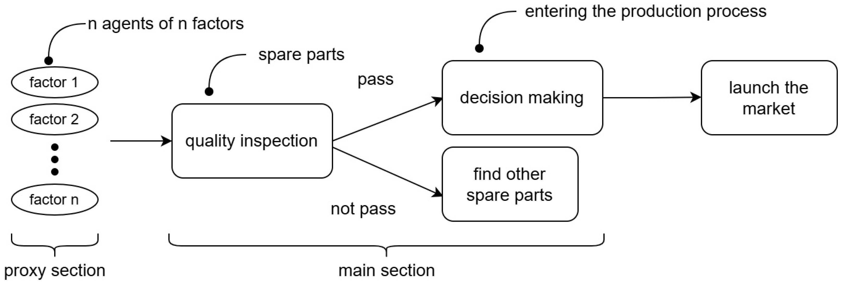
Figure 1.
Flowchart of the decision-making process in the proposed multi-agent mixed-integer programming model, highlighting key steps, such as component inspection, decision node interaction, and cost-based path evaluation.
Figure 1.
Flowchart of the decision-making process in the proposed multi-agent mixed-integer programming model, highlighting key steps, such as component inspection, decision node interaction, and cost-based path evaluation.
Figure 2.
Schematic overview of the production process, including spare part procurement, quality inspection, assembly, and the disassembly of defective products.
Figure 2.
Schematic overview of the production process, including spare part procurement, quality inspection, assembly, and the disassembly of defective products.
Figure 3.
Diagram of the single-stage production decision model. Each decision variable (inspection, disassembly) corresponds to binary options used in the optimization.
Figure 3.
Diagram of the single-stage production decision model. Each decision variable (inspection, disassembly) corresponds to binary options used in the optimization.
Figure 4.
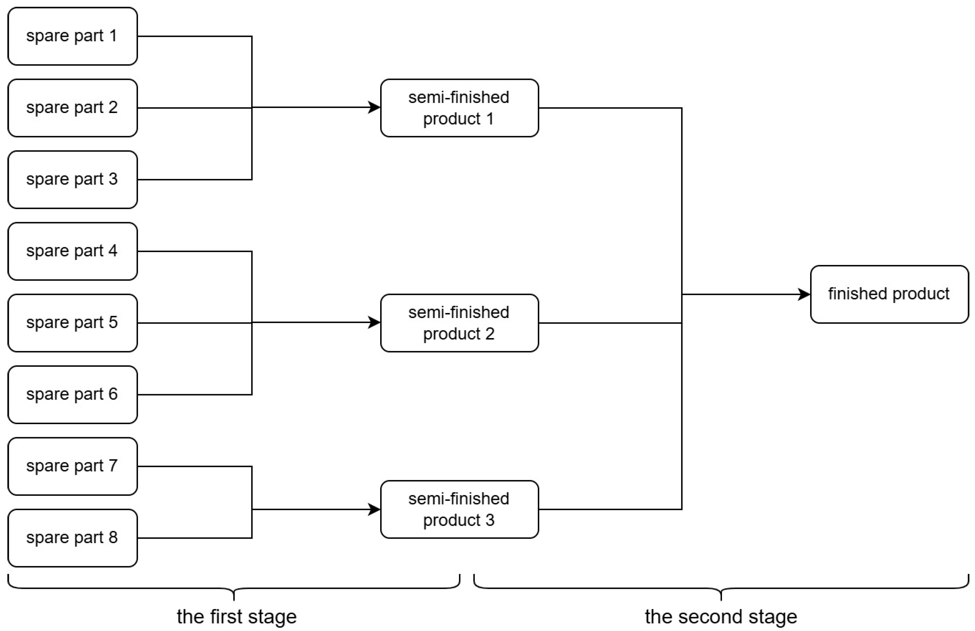
Multistage production model structure involving sequential decision points for semi-finished and finished products, allowing analysis of cumulative cost and inspection strategies.
Figure 4.
Multistage production model structure involving sequential decision points for semi-finished and finished products, allowing analysis of cumulative cost and inspection strategies.
Figure 5.
Variation in the required sample size n with respect to different actual defect rates at a 95% confidence level, based on normal approximation for binomial distribution.
Figure 5.
Variation in the required sample size n with respect to different actual defect rates at a 95% confidence level, based on normal approximation for binomial distribution.
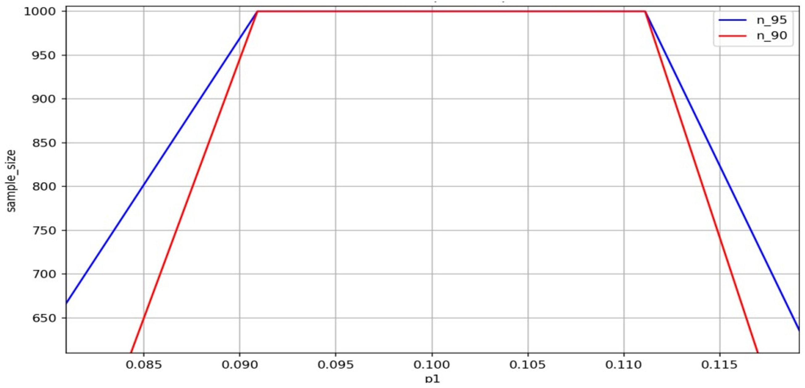
Figure 6.
Detailed view of sample size n behavior within the critical range , where values plateau due to exceeding batch size.
Figure 6.
Detailed view of sample size n behavior within the critical range , where values plateau due to exceeding batch size.
Figure 7.
Required sample size n at a 95% confidence level when the actual defect rate exceeds the nominal rate.
Figure 7.
Required sample size n at a 95% confidence level when the actual defect rate exceeds the nominal rate.
Figure 8.
Required sample size n at a 90% confidence level when the actual defect rate does not exceed the nominal rate.
Figure 8.
Required sample size n at a 90% confidence level when the actual defect rate does not exceed the nominal rate.
Figure 9.
The Monte Carlo simulation of rejection rate for , at 95% confidence.
Figure 9.
The Monte Carlo simulation of rejection rate for , at 95% confidence.
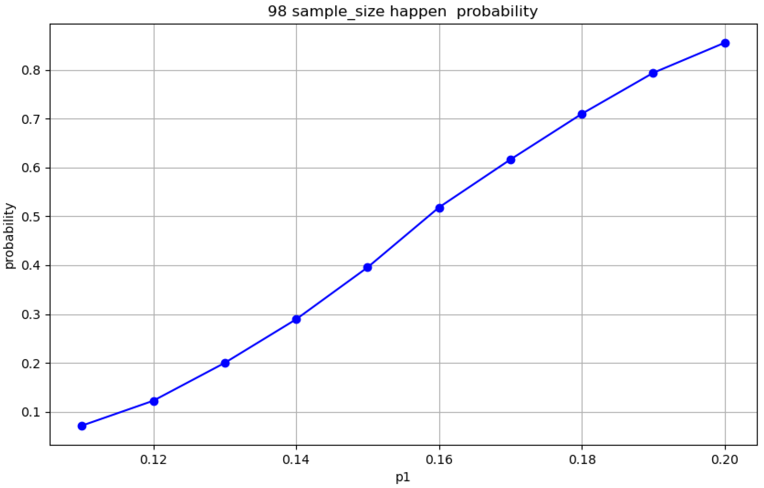
Figure 10.
The Monte Carlo simulation of rejection accuracy at , , 95% confidence.
Figure 10.
The Monte Carlo simulation of rejection accuracy at , , 95% confidence.
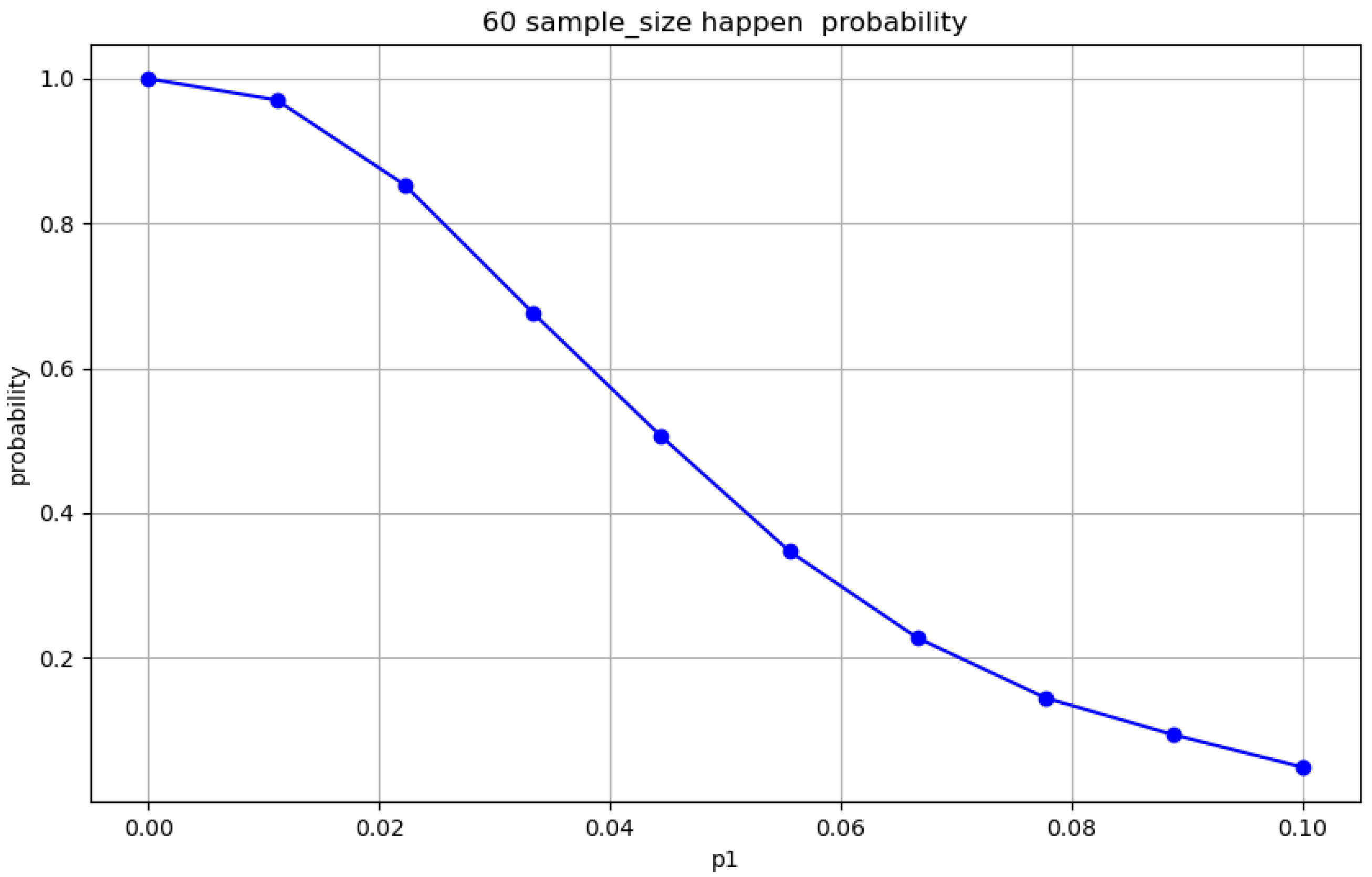
Figure 11.
Acceptance Monte Carlo simulation at , , 90% confidence.
Figure 11.
Acceptance Monte Carlo simulation at , , 90% confidence.
Figure 12.
Acceptance Monte Carlo simulation at , , 90% confidence.
Figure 12.
Acceptance Monte Carlo simulation at , , 90% confidence.
Figure 13.
Surface plots illustrating the impact of nominal defect rate and sample size on estimated defect probability under different settings: (a,b) Surface plot of as a function of and . (c,d) Surface plot of as a function of .
Figure 13.
Surface plots illustrating the impact of nominal defect rate and sample size on estimated defect probability under different settings: (a,b) Surface plot of as a function of and . (c,d) Surface plot of as a function of .
Figure 14.
Graphical representation of how the average estimated defect rate varies with sample size and initial value , with random fluctuations added: (a) Plot of versus the average sample size considering random errors. (b) Plot of versus the initial probability considering random errors.
Figure 14.
Graphical representation of how the average estimated defect rate varies with sample size and initial value , with random fluctuations added: (a) Plot of versus the average sample size considering random errors. (b) Plot of versus the initial probability considering random errors.
Table 1.
Input parameters for single-stage decision model under six scenarios. This table lists the defect rates, purchase prices, detection costs, assembly costs, market prices, and replacement losses for spare parts and finished products in six single-stage production scenarios. These inputs are used to evaluate inspection and disassembly strategies.
| S | SP1 | SP2 | FP | DFP |
|---|
| DR |
PP
|
DC
|
DR
|
PP
|
DC
|
DR
|
AC
|
DC
|
MP
| SL | DC |
|---|
| 1 | 10% | 4 | 2 | 10% | 18 | 3 | 10% | 6 | 3 | 56 | 6 | 5 |
| 2 | 20% | 4 | 2 | 20% | 18 | 3 | 20% | 6 | 3 | 56 | 6 | 5 |
| 3 | 10% | 4 | 2 | 10% | 18 | 3 | 10% | 6 | 3 | 56 | 30 | 5 |
| 4 | 20% | 4 | 1 | 20% | 18 | 1 | 20% | 6 | 2 | 56 | 30 | 5 |
| 5 | 10% | 4 | 8 | 20% | 18 | 1 | 10% | 6 | 2 | 56 | 10 | 5 |
| 6 | 5% | 4 | 2 | 5% | 18 | 3 | 5% | 6 | 3 | 56 | 10 | 40 |
Table 2.
Input data for multistage decision model: components, semi-finished products, and final assembly. Provides parameter values including defect rates, purchase prices, and process costs for components and semi-finished products used in multistage production simulations.
Table 2.
Input data for multistage decision model: components, semi-finished products, and final assembly. Provides parameter values including defect rates, purchase prices, and process costs for components and semi-finished products used in multistage production simulations.
| SP | DR | PP | DC | SFP | DR | AC | DC | DC |
|---|
| 1 | 10% | 2 | 1 | 1 | 10% | 8 | 4 | 6 |
| 2 | 10% | 8 | 1 | 2 | 10% | 8 | 4 | 6 |
| 3 | 10% | 12 | 2 | 3 | 10% | 8 | 4 | 6 |
| 4 | 10% | 2 | 1 | | | | | |
| 5 | 10% | 8 | 1 | FP | 10% | 8 | 6 | 10 |
| 6 | 10% | 12 | 2 | | | | | |
| 7 | 10% | 8 | 1 | | | MP | | SL |
| 8 | 10% | 12 | 2 | FP | | 200 | | 40 |
Table 3.
Optimal decision strategies and performance metrics in single-stage scenarios. Shows the resulting inspection and disassembly decisions, total cost, and expected profit for each of the six single-stage cases based on integer programming.
Table 3.
Optimal decision strategies and performance metrics in single-stage scenarios. Shows the resulting inspection and disassembly decisions, total cost, and expected profit for each of the six single-stage cases based on integer programming.
| S | SP1 I | SP2 I | FPI | N D | MC | MP |
|---|
| 1 | No | No | No | No | 34.60 | 21.40 |
| 2 | No | No | No | No | 35.20 | 20.79 |
| 3 | No | No | No | No | 37.00 | 19.00 |
| 4 | Yes | Yes | Yes | Yes | 35.59 | 20.40 |
| 5 | No | No | Yes | Yes | 34.80 | 21.20 |
| 6 | No | No | No | No | 34.50 | 21.50 |
Table 4.
First stage decision outcomes and metrics for multistage framework presents inspection/disassembly decisions, costs, and profits for spare part processing in the first stage of a multistage production path.
Table 4.
First stage decision outcomes and metrics for multistage framework presents inspection/disassembly decisions, costs, and profits for spare part processing in the first stage of a multistage production path.
| Situations | Spare Part 1 Inspection | Spare Part 2 Inspection | Finished Product Inspection | Nonconforming Disassembly | Minimum Cost | Maximum Profit |
|---|
| 1 | No | No | No | No | 34.60 | 21.40 |
| 2 | No | No | No | No | 35.20 | 20.79 |
| 3 | No | No | No | No | 37.00 | 19.00 |
| 4 | Yes | Yes | Yes | Yes | 35.59 | 20.40 |
| 5 | No | No | Yes | Yes | 34.80 | 21.20 |
| 6 | No | No | No | No | 34.50 | 21.50 |
Table 5.
Second stage optimization results: from semi-finished to final products. Summarizes decisions regarding finished product inspection and disassembly, along with resulting costs.
Table 5.
Second stage optimization results: from semi-finished to final products. Summarizes decisions regarding finished product inspection and disassembly, along with resulting costs.
| Process | Case | Finished Product Inspection | Nonconforming Finished Product Disassembly | Minimum Cost |
|---|
| Second process | Semi-finished to finished product | No | No | 36 |
Table 6.
Estimated Defect Rates and Confidence Intervals for Spare Parts . Lists empirical defect rate estimates and corresponding confidence intervals for individual components under increased nominal defect assumptions.
Table 6.
Estimated Defect Rates and Confidence Intervals for Spare Parts . Lists empirical defect rate estimates and corresponding confidence intervals for individual components under increased nominal defect assumptions.
| Component | Defective Rate | Confidence Interval |
|---|
| 1 | 0.216835 | [0.201672, 0.244998] |
| 2 | 0.226246 | [0.199464, 0.242631] |
| 3 | 0.210470 | [0.193402, 0.236122] |
| 4 | 0.231982 | [0.199149, 0.242294] |
| 5 | 0.220272 | [0.204925, 0.248482] |
| 6 | 0.217769 | [0.205233, 0.248812] |
| 7 | 0.208167 | [0.199922, 0.243123] |
| 8 | 0.217100 | [0.192996, 0.235686] |
Table 7.
Estimated Defect Rates and Confidence Intervals for Semi-Finished and Finished Products. Provides statistical summaries of quality inspection results at later stages in production under nominal defect rate .
Table 7.
Estimated Defect Rates and Confidence Intervals for Semi-Finished and Finished Products. Provides statistical summaries of quality inspection results at later stages in production under nominal defect rate .
| Type | Defect Rate | Confidence Interval |
|---|
| Semi-finished product 1 | 0.070905 | [0.070302, 0.100449] |
| Semi-finished product 2 | 0.087885 | [0.089550, 0.121511] |
| Semi-finished product 3 | 0.092422 | [0.078420, 0.108716] |
| Finished product | 0.077132 | [0.066338, 0.094639] |
Table 8.
First stage decision results under elevated nominal defect rate . Summarizes inspection and disassembly choices, as well as costs, for spare parts in the first stage under revised defect rate assumptions.
Table 8.
First stage decision results under elevated nominal defect rate . Summarizes inspection and disassembly choices, as well as costs, for spare parts in the first stage under revised defect rate assumptions.
| P | C | SP1 I | SP2 I | SP3 I | SF I | N/SF D | MC |
|---|
| | SFP 1 | No | Yes | Yes | No | No | 44.455348 |
| FP | SFP 2 | No | Yes | Yes | No | No | 44.381960 |
| | SFP 3 | No | Yes | / | No | No | 35.334664 |
Table 9.
Second stage decision outcomes for final assembly under elevated defect rate . Details whether to inspect or disassemble final products, along with associated costs, under updated quality conditions.
Table 9.
Second stage decision outcomes for final assembly under elevated defect rate . Details whether to inspect or disassemble final products, along with associated costs, under updated quality conditions.
| Process | Case | Finished Product Inspection | Nonconforming Finished Product Disassembly | Minimum Cost |
|---|
| Second Process | Semi-finished to Finished Product | No | Yes | 35.334664 |
Table 10.
Comparison of decision tree outcomes for single-stage production. Compares final decisions, profits, and costs under a traditional decision tree approach to highlight differences from the proposed model.
Table 10.
Comparison of decision tree outcomes for single-stage production. Compares final decisions, profits, and costs under a traditional decision tree approach to highlight differences from the proposed model.
| Spare Part 1 | Spare Part 2 | Finished Product | Final Profit | Final Cost |
|---|
|
Detection
|
Disassembly
|
Detection
|
Disassembly
|
Detection
|
Disassembly
|
|---|
| Yes | No | Yes | No | Yes | No | 9 | 53 |
| Yes | No | Yes | No | Yes | Yes | 9 | 53 |
| No | No | Yes | No | Yes | No | −15 | 101 |
| Yes | Yes | Yes | Yes | Yes | Yes | −11 | 97 |
| Yes | No | Yes | Yes | Yes | No | 2 | 64 |
| No | No | No | No | Yes | No | −30 | 96 |
Table 11.
Comparison of decision tree outcomes for single-stage production. Compares final decisions, profits, and costs under a traditional decision tree approach to highlight differences from the proposed model.
Table 11.
Comparison of decision tree outcomes for single-stage production. Compares final decisions, profits, and costs under a traditional decision tree approach to highlight differences from the proposed model.
| Spare Part | Detection Decision | Disassembly Decision | Cost |
|---|
| 1 | Yes | Yes | 9 |
| 2 | Yes | Yes | 15 |
| 3 | Yes | Yes | 20 |
| 4 | Yes | Yes | 9 |
| 5 | Yes | Yes | 15 |
| 6 | Yes | Yes | 20 |
| 7 | Yes | Yes | 15 |
| 8 | Yes | No | 54 |
Table 12.
Decision tree-based actions for semi-finished product processing. Summarizes inspection and disassembly strategies applied to semi-finished products and associated costs.
Table 12.
Decision tree-based actions for semi-finished product processing. Summarizes inspection and disassembly strategies applied to semi-finished products and associated costs.
| Semi-Finished Production | Detection Decision | Disassembly Decision | Cost |
|---|
| 1 | Yes | Yes | 14 |
| 2 | Yes | Yes | 14 |
| 3 | Yes | Yes | 14 |
Table 13.
Decision tree-based final product processing and performance indicators. Presents outcomes for finished product inspection and disassembly, along with cost and profit results, under a decision tree framework.
Table 13.
Decision tree-based final product processing and performance indicators. Presents outcomes for finished product inspection and disassembly, along with cost and profit results, under a decision tree framework.
| Detection Decision | Disassembly Decision | Cost | Profit |
|---|
| Yes | No | 218 | −18.0 |
Table 14.
Estimated defect rates of eight components from batch sampling . Lists point estimates of defect rates for all components used in the case study based on empirical inspection.
Table 14.
Estimated defect rates of eight components from batch sampling . Lists point estimates of defect rates for all components used in the case study based on empirical inspection.
| Part Number | Defect Rate |
|---|
| 1 | 0.106928 |
| 2 | 0.114761 |
| 3 | 0.128279 |
| 4 | 0.112093 |
| 5 | 0.105622 |
| 6 | 0.119404 |
| 7 | 0.094784 |
| 8 | 0.117643 |
Table 15.
Estimated Defect Rates for Semi-Finished and Finished Products in Case Study. Reports updated defect rate estimates for higher-level products based on batch inspection under nominal quality thresholds.
Table 15.
Estimated Defect Rates for Semi-Finished and Finished Products in Case Study. Reports updated defect rate estimates for higher-level products based on batch inspection under nominal quality thresholds.
| Type | Defect Rate |
|---|
| Semi-finished Product 1 | 0.070905 |
| Semi-finished Product 2 | 0.087885 |
| Semi-finished Product 3 | 0.092422 |
| Finished Product | 0.077132 |
Table 16.
Decision results for Stage 1 component processing based on sampled defect Rates. Indicates optimized inspection and disassembly decisions and related costs for each component set in the first process stage.
Table 16.
Decision results for Stage 1 component processing based on sampled defect Rates. Indicates optimized inspection and disassembly decisions and related costs for each component set in the first process stage.
| P | C | SP1 I | SP2 I | SP3 I | SF I | N/SF D | MC |
|---|
| | SFP 1 | No | No | No | No | No | 46.00 |
| FP | SFP 2 | No | No | No | No | No | 46.00 |
| | SFP 3 | No | No | / | No | No | 36.00 |
Table 17.
Optimized Stage 2 decisions for semi-finished to final product conversion. Shows whether inspection and disassembly are selected for finished products, and total cost incurred during final assembly.
Table 17.
Optimized Stage 2 decisions for semi-finished to final product conversion. Shows whether inspection and disassembly are selected for finished products, and total cost incurred during final assembly.
| Process | Case | Finished Product Inspection | Nonconforming Finished Product Disassembly | Minimum Cost |
|---|
| Second process | Semi-finished to finished product | No | No | 36 |


