Denoising Autoencoder and Contrast Enhancement for RGB and GS Images with Gaussian Noise

Abstract

Robust image processing systems require input images that closely resemble real-world scenes. However, external factors, such as adverse environmental conditions or errors in data transmission, can alter the captured image, leading to information loss. These factors may include poor lighting conditions at the time of image capture or the presence of noise, necessitating procedures to restore the data to a representation as close as possible to the real scene. This research project proposes an architecture based on an autoencoder capable of handling both poor lighting conditions and noise in digital images simultaneously, rather than processing them separately. The proposed methodology has been demonstrated to outperform competing techniques specialized in noise reduction or contrast enhancement. This is supported by both objective numerical metrics and visual evaluations using a validation set with varying lighting characteristics. The results indicate that the proposed methodology effectively restores images by improving contrast and reducing noise without requiring separate processing steps.

1. Introduction

Gaussian noise is one of the most common types of noise observed in digital images, often introduced during image acquisition due to various factors. These factors include adverse lighting conditions, thermal instabilities in camera sensors, and failures in the electronic structure of the camera [1]. Adverse lighting conditions have been shown to degrade the visual quality of digital images and exacerbate the noise inherent to camera sensors, thereby increasing the presence of Gaussian noise in the captured image.

The term “adverse lighting conditions” refers to two specific scenarios: low illumination and high illumination. In the case of low illumination, the resulting digital image exhibits reduced brightness and low contrast [2]. Additionally, within the electronic structure of the camera, sensors exhibit increased sensitivity to weak signals, amplifying any signal variations and resulting in the generation of Gaussian noise. Conversely, under high illumination conditions, the camera sensors become saturated, leading to a nonlinear response in the captured data [3] and contributing to the presence of Gaussian noise. Moreover, the heat generated, along with other types of noise, such as thermal noise, further affects the image quality.

Several techniques have been developed to mitigate the impact of Gaussian noise in images captured under poor lighting conditions. These include both classical image processing methods and advanced deep learning-based approaches [4]. Some of these techniques focus on separately addressing noise reduction and illumination enhancement [5]. However, it is important to distinguish between illumination enhancement and contrast enhancement as they are two distinct techniques in image processing that address different aspects of a visual quality of the image. While illumination enhancement adjusts the overall brightness to improve visibility and make the image clearer and easier to interpret [6], contrast enhancement increases the difference between light and dark areas to make details more perceptible [7]. This research highlights the importance of simultaneously enhancing image details through contrast adjustment and reducing noise using an autoencoder neural network. This is achieved by analyzing the image and applying trained models based on the features present in the input data.

Section 2 presents and analyzes the relevant theoretical background. The proposed model is described in Section 3, while the experimental setup and results are discussed in Section 4. Finally, the conclusions of this research work are provided in Section 5.

2. Background Work

Inadequate lighting during scene capture can lead to several issues that negatively impact the visual quality of an image. These issues range from underexposure or oversaturation to noise generation, as illustrated in Figure 1 (derived from Smartphone Image Denoising Dataset (SIDD) [8]).

Noise in digital images refers to variations in pixel values that distort the original information. This alteration can occur during image capture, digitization, storage, or transmission. Different types of noise are characterized by how they interact with the image and can be identified based on their source. One of the most common types of noise in images is Gaussian noise. Various techniques, both traditional and deep learning-based, have been developed to reduce this type of noise. Traditional approaches include methods such as the median filter [9], while deep learning techniques have an inherent ability to overcome the limitations of certain conventional algorithms, such as the following:

• Denoising Convolutional Neural Network (DnCNN): This study introduced the design of a Convolutional Neural Network (CNN) specifically developed to reduce Gaussian noise in digital images. The network consists of multiple convolutional layers, followed by batch normalization and ReLU activation functions. A distinctive feature of this architecture is that it does not directly learn to generate a denoised image; instead, it employs residual learning, where the model learns to predict the difference between the noisy image and its denoised counterpart. This approach facilitates learning and improves model convergence [10].
• Nonlinear Activation Free Network (NAFNet): This study presented an alternative $CNN$ designed for image denoising. The network was developed with the objective of improving architectural efficiency and simplifying computations by minimizing the use of nonlinear activation functions, such as Rectified Linear Unit (ReLU). This design choice enhances computational efficiency while maintaining optimal model performance [11].
• Restoration Transformer (Restormer): This network is based on the Transformer architecture and is specifically designed for image restoration tasks, including Gaussian noise reduction. This approach leverages the advantages of Transformer networks to optimize memory usage and computational efficiency while simultaneously capturing long-range dependencies [12].

In the context of digital images, contrast is defined as the measure of the difference between the brightness levels of the lightest and darkest areas in an image. Adequate contrast enhances the visual quality of an image, whereas insufficient contrast can result in a visually flat appearance [7]. To address the issue of poor contrast in images, several algorithms have been developed in recent years to enhance contrast. Examples include An Advanced Whale Optimization Algorithm for Grayscale Image Enhancement [13], Pixel Intensity Optimization and Detail-Preserving Contextual Contrast Enhancement for Underwater Images [14], and Optimal Bezier Curve Modification Function for Contrast-Degraded Images [15]. However, these algorithms primarily focus on enhancing specific image channels or improving images under a single lighting condition.

Some algorithms that operate across all image channels and are capable of functioning under extreme lighting conditions, whether in low or high illumination, include the following:

• Single-Scale Retinex (SSR) is a technique designed to enhance the contrast and illumination of digital images. It is based on human perception of color and luminance in real-world scenes, simulating how the human eye adapts to different lighting conditions by adjusting color perception and scene illumination [16]. The application process of $SSR$ is outlined in Equations (1)–(6).

  $$I(x,y)=R(x,y)·L(x,y),$$

  (1)

  where $I(x,y)$ represents the original image pixel, which can be decomposed into two components: $R(x,y)$, the reflectance component; and $L(x,y)$, the illumination component.
  To facilitate the distinction between reflectance and illumination, the following logarithmic transformation is applied:

  $$logI(x,y)=logR(x,y)+logL(x,y).$$

  (2)
  Clarity enhancement is achieved by applying a Gaussian filter to smooth the original image:

  $$L(x,y)\approx \widehat{L}(x,y)=F(x,y)\ast I(x,y),$$

  (3)

  where $F(x,y)$ is the Gaussian filter, and ∗ denotes two-dimensional convolution, which is formally defined as follows:

  $$(f\ast g)(x,y)={\int }_{-\infty }^{\infty }{\int }_{-\infty }^{\infty }F(x-\alpha ,y-\beta )I(\alpha ,\beta )d\alpha d\beta .$$

  (4)
  The reflectance component $R(x,y)$ is obtained by subtracting the illumination component in the logarithmic domain:

  $$\widehat{R}(x,y)=logI(x,y)-log\widehat{L}(x,y).$$

  (5)
  Finally, an inverse transformation is performed to reconstruct the processed image:

  $$I_{SSR}=exp\left(\widehat{R}(x,y)\right).$$

  (6)
• Multiscale Retinex (MSR) is an extension of the $SSR$ algorithm, and it was designed to overcome the limitations of Gaussian filter scale sensitivity. Unlike $SSR$, this algorithm operates across multiple filter scales, utilizing the results from different scales to achieve a balance between local and global details [17]. The computation of $MSR$ is given by Equation (7).

  $$R_{MSR}(x,y)=\sum _{i=1}^n{W}_i·logI(x,y)-\left[F_i(x,y)\ast I(x,y)\right],$$

  (7)

  where $R_{MSR}(x,y)$ represents the output value at coordinates $(x,y)$, n is the number of scales, and $W_i$ and $F_i$ denote the weight and the Gaussian filter at scale i, respectively.
• Multiscale Retinex with Color Restoration (MSRCR) is an enhancement of the $MSR$ algorithm that combines the contrast and detail enhancement capabilities of $MSR$ with a function designed to preserve the natural colors of the image, thereby preventing the loss of color fidelity [18]. The computation of $MSRCR$ is described in Equations (8) and (9).

  $$R_{MSRCR}(x,y)=C(x,y)·R_{MSR}(x,y),$$

  (8)

  $$C(x,y)=\beta ·log\left(1+{\displaystyle \frac{I(x,y)}{{\sum }_k{I}_k(x,y)}}\right),$$

  (9)

  where $R_{MSRCR}(x,y)$ represents the output value at coordinates $(x,y)$, $C(x,y)$ is the color restoration function, $\beta$ is a gain-related constant, and $I_k(x,y)$ corresponds to the pixel intensity in the k different channels of the image.
• Multiscale Retinex with Chromaticity Preservation (MSRCP) is a refinement of $MSR$, and it was designed to preserve the chromaticity of the image while enhancing its contrast and detail. This approach ensures a more faithful representation of the original colors [18]. The computation of $MSRCP$ is described in Equations (10)–(12).

  $$I_A(x,y)={\displaystyle \frac{R(x,y)+G(x,y)+B(x,y)}{3}},$$

  (10)

  $$C_k(x,y)={\displaystyle \frac{I_k(x,y)}{I_A(x,y)}},k\in R,G,B,$$

  (11)

  $$R_{MSRCP}(x,y)=C_k(x,y)·R_{MSR}(x,y),$$

  (12)

  where $I_A(x,y)$ represents the average intensity of the pixel at coordinates $(x,y)$, $C_k(x,y)$ denotes the chromatic proportions, and $R_{MSRCP}(x,y)$ is the resulting value.
• Gamma correction is a technique used to enhance the brightness and contrast of a digital image. It adjusts the relationship between intensity levels and their perceived brightness, thereby helping to correct distortions [19]. The computation of Gamma correction is given by Equation (13).

  $$S=I^{\gamma },$$

  (13)

  where S represents the output intensity, I is the input intensity, and $\gamma$ is the correction factor.
• Histogram equalization is a widely used algorithm for contrast enhancement. It improves contrast by redistributing intensity levels (Equation (14)) so that the histogram approaches a uniform distribution. This process enhances details in low-contrast images.

  $$S=(L-1)p\left(I\right),$$

  (14)

  where L represents the maximum intensity value in the image, and $p\left(I\right)$ is the probability of an event occurring at that intensity.

3. Proposed Model

The aforementioned algorithms have been shown to prioritize a single objective, either noise reduction or contrast enhancement. However, a new algorithm is proposed that performs both tasks simultaneously, yielding superior results compared to existing methods. The proposed algorithm, Denoising Vanilla Autoencoder with Contrast Enhancement (DVACE), was designed to simultaneously address the noise reduction and contrast enhancement in images represented mathematically as multidimensional arrays. First, consider an original image X, defined as a two-dimensional matrix (Gray Scale (GS) image) or a three-dimensional tensor (Red, Green, Blue (RGB) image), where each matrix entry corresponds to the pixel intensity at position $(i,j)$.

Then, let the original multidimensional image be the following:

$$X\in {\mathbb{R}}^{M\times N\times C},$$

(15)

where $M\times N$ is the spatial resolution of the image, C is the number of channels ($C=1$ for GS, and $C=3$ for RGB).

Considering a multidimensional Gaussian noise model [20], the observed noisy image is expressed as follows:

$$Y=X+\eta ,\mathrm{with}\eta \sim \mathcal{N}(\overline{\mathit{X}},\mathsf{\Sigma }),$$

(16)

where $Y\in {\mathbb{R}}^{M\times N\times C}$ is the observed noisy image, $X\in {\mathbb{R}}^{M\times N\times C}$ is the original noise-free image, $\eta \in {\mathbb{R}}^{M\times N\times C}$ is additive Gaussian noise, $\overline{\mathit{X}}$ is the multidimensional mean matrix (local or global) of pixels, and $\mathsf{\Sigma }$ is the covariance matrix representing the multidimensional noise dispersion (typically $\mathsf{\Sigma }={\sigma }^{2}I$ for stationary, uncorrelated noise between pixels and channels, where I is the multidimensional identity matrix).

For each pixel at a specific position $(i,j)$ with observed value ${\mathbf{y}}_{ij}$ (vector for RGB and scalar for GS), the Gaussian noise probability distribution is as follows:

$$P\left({\mathbf{y}}_{ij}\right)={\displaystyle \frac{1}{\sqrt{{\left(2\pi \right)}^C\left|\mathsf{\Sigma }\right|}}}exp\left(-{\displaystyle \frac{1}{2}}{({\mathbf{y}}_{ij}-{\overline{\mathit{x}}}_{ij})}^T{\mathsf{\Sigma }}^{-1}({\mathbf{y}}_{ij}-{\overline{\mathit{x}}}_{ij})\right),$$

(17)

where ${\mathbf{y}}_{ij}$ is the column vector (for RGB and $C=3$), the scalar (GS, $C=1$) is observed at spatial position $(i,j)$, ${\overline{\mathit{x}}}_{ij}$ is the original local mean at position $(i,j)$, and $\mathsf{\Sigma }$ is the noise covariance matrix (simplified often to $\mathsf{\Sigma }={\sigma }^2{I}_C$, with $I_C$ as the $C\times C$ identity matrix).

If noise is stationary and isotropic (equal in all directions), the equation simplifies to the following:

$$P\left({\mathbf{y}}_{ij}\right)={\displaystyle \frac{1}{{\left(2\pi {\sigma }^2\right)}^{C/2}}}exp\left(-{\displaystyle \frac{\parallel {\mathbf{y}}_{ij}-{\overline{\mathit{x}}}_{ij}{\parallel }_2^2}{2{\sigma }^2}}\right).$$

(18)

The joint probability for the entire observed image, assuming independence among pixels and channels, is as follows:

$$P\left(Y\right|X)=\prod _{i=1}^M\prod _{j=1}^{N}P\left({\mathbf{y}}_{ij}\right)={\displaystyle \frac{1}{{\left(2\pi {\sigma }^2\right)}^{MNC/2}}}exp\left(-{\displaystyle \frac{1}{2{\sigma }^2}}\sum _{i=1}^M\sum _{j=1}^N{\parallel {\mathbf{y}}_{ij}-{\overline{\mathit{x}}}_{ij}\parallel }_2^2\right).$$

(19)

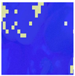
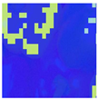
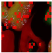
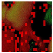
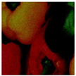
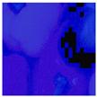
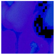
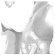
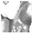
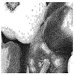
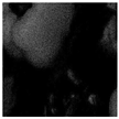
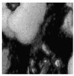
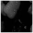
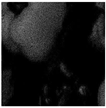
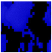
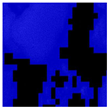
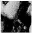
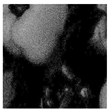
This provides the mathematical foundation on which the DVACE model optimizes the estimation of the original image X by minimizing the exponential term that represents the squared error between the observed noisy image Y and the restored image X. By adjusting the variance, the density of noise present in the image can be increased or decreased. Additionally, by modifying the mean, the image can appear underexposed (Figure 2a) or overexposed (Figure 2b). This demonstrates how the illumination of the image changes, either darkening or brightening. Finally, the histogram corresponding to the simulated image is presented.

Figure 3 presents the flowchart of the proposed model architecture for RGB images, while Figure 4 shows the flowchart of the proposed model architecture for GS images.

Each architecture calculates the Signal-to-Noise Ratio (SNR) of the input image. The SNR metric [21] is used to enhance the network’s ability to determine the most suitable model—whether to apply a model that brightens dark images or one that darkens bright images—during the actual processing stage. The SNR is defined for an image $\mathbf{X}\in {\mathbb{R}}^{w\times h\times c}$, where $w,h,$ and c represent the spatial and channel dimensions. The SNR quantifies the mean intensity relative to the variance in the image:

$$\mathrm{SNR}={\displaystyle \frac{\mathbb{E}\left[\mathbf{X}\right]}{\sqrt{\mathrm{Var}\left[\mathbf{X}\right]}}},$$

(20)

where the mean and the variance are computed as follows:

$$\mathbb{E}\left[\mathbf{X}\right]={\displaystyle \frac{1}{whc}}\sum _{i=0}^w\sum _{j=0}^h\sum _{k=0}^{c}X(i,j,k),$$

(21)

$$\mathrm{Var}\left[\mathbf{X}\right]={\displaystyle \frac{1}{whc}}\sum _{i=0}^w\sum _{j=0}^h\sum _{k=0}^c{\left(X(i,j,k)-\mathbb{E}\left[\mathbf{X}\right]\right)}^2.$$

(22)

This formulation provides a robust measure of the image intensity relative to its noise distribution. It is evident that the design of Algorithms 1 and 2 was based on the proposed architectures.

The SNR thresholds used in both the RGB and GS algorithms were determined experimentally by calculating the average SNR of the corrupted images used to train the network. Equations (23)–(31) illustrate the DVACE procedure.   

Given a set of images in different modalities ($X_{GS}$ for GS images and $X_{RGB}$ for RGB images), the classification process based on the SNR can be rigorously expressed as a decision function, which is defined as follows:

$${\mathbf{X}}^{\prime }=\left\{\begin{array}{cc}{f}_{\mathrm{Unimodal}}\left(\mathbf{X}\right)\hfill & \mathrm{if}\mathbf{X}\in {\mathbb{R}}^{M\times N},\mathrm{and}SNR\left(\mathbf{X}\right)\le {\tau }_{GS}\hfill \\ g_{\mathrm{Unimodal}}\left(\mathbf{X}\right)\hfill & \mathrm{if}\mathbf{X}\in {\mathbb{R}}^{M\times N},\mathrm{and}SNR\left(\mathbf{X}\right)>{\tau }_{GS}\hfill \\ f_{\mathrm{Multimodal}}\left(\mathbf{X}\right)\hfill & \mathrm{if}\mathbf{X}\in {\mathbb{R}}^{M\times N\times C},\mathrm{and}SNR\left(\mathbf{X}\right)\le {\tau }_{RGB}\hfill \\ g_{\mathrm{Multimodal}}\left(\mathbf{X}\right)\hfill & \mathrm{if}\mathbf{X}\in {\mathbb{R}}^{M\times N\times C},\mathrm{and}SNR\left(\mathbf{X}\right)>{\tau }_{RGB}\hfill \end{array}\right.,$$

(23)

where X represents the input image; $X^{\prime }$ is the processed image by the DVACE model; ${\mathbb{R}}^{M\times N}$ represents the GS image space; ${\mathbb{R}}^{M\times N\times C}$ represents the RGB image space with C channels; $SNR\left(X\right)$ is the function computing the SNR of the image; and ${\tau }_{GS}=2.6$ and ${\tau }_{RGB}=1.73$ are predefined SNR thresholds for GS and RGB images, respectively.

$f_{\mathrm{Unimodal}}$ and $g_{\mathrm{Unimodal}}$ are the unimodal enhancement functions for GS images, and the following apply:

• $f_{\mathrm{Unimodal}}\left(X\right)$ is applied to images with low SNR (dark images).
• $g_{\mathrm{Unimodal}}\left(X\right)$ is applied to images with high SNR (bright images).

$f_{\mathrm{Multimodal}}$ and $g_{\mathrm{Multimodal}}$ are the multimodal enhancement functions for RGB images, and the following apply:

• $f_{\mathrm{Multimodal}}\left(X\right)$ is applied to images with low SNR (dark images).
• $g_{\mathrm{Multimodal}}\left(X\right)$ is applied to images with high SNR (bright images).

The convolutional operation ∗ between an input tensor $\mathbf{X}$ and a kernel $\mathbf{W}\in {\mathbb{R}}^{m\times n\times c\times k}$ is defined as follows:

$${(\mathbf{X}\ast \mathbf{W})}_{(i,j,k)}=\sum _{m=0}^{M-1}\sum _{n=0}^{N-1}\sum _{c=0}^{C-1}X(i+m-\Delta ,j+n-\Delta ,c)·W_{(m,n,c,k)}+b_k,$$

(24)

where $\Delta =\lfloor M/2\rfloor$ accounts for padding in the kernel size, and $b_k$ is the bias term for channel k.

A non-linear transformation is applied to the convolutional result:

$$Y_{(i,j,k)}=\varphi \left({(\mathbf{X}\ast \mathbf{W})}_{(i,j,k)}\right),$$

(25)

where the activation function $\varphi$ is defined as follows:

$$\varphi \left(x\right)=max(0,x),$$

(26)

this introduces non-linearity, enabling feature extraction from high-dimensional spaces.

Dimensional reduction is performed through max-pooling:

$$Z_{(i,j,k)}=\underset{0\le p^{\prime }\le P,0\le q^{\prime }\le Q}{max}{Y}_{(i+p^{\prime },j+q^{\prime },k)},$$

(27)

where $P,Q$ define the pooling window size. This operation selects the most dominant feature per region.

A secondary convolutional pass refines the extracted features:

$$Z_{(i,j,k)}^{\prime }=\varphi \left(Z\ast {\mathbf{W}}^{\prime }\right),$$

(28)

where ${\mathbf{W}}^{\prime }$ represents a new set of learned weights.

To restore spatial resolution, we applied weighted bilinear interpolation:

$$\sum _{0\le p^{\prime }\le P,0\le q^{\prime }\le Q}\left\{w_n·Y_{(i+p^{\prime },j+q^{\prime },k)}^{\prime }\right\}=Z_{(i,j,k)}^{\prime },$$

(29)

where $w_n$ are interpolation weights satisfying the following:

$$\sum _n{w}_n=1.$$

(30)

A final convolutional step reconstructs the enhanced image as follows:

$$X_{(i,j,k)}^{\prime }={(Y^{\prime }\ast {\mathbf{W}}^{″})}_{(i,j,k)},$$

(31)

where ${\mathbf{W}}^{″}$ represents a final learned weight set for output feature mapping.

Following the Denoising Vanilla Autoencoder (DVA) training structure and methodology [22], two databases were created using images from the “1 Million Faces” dataset [23], from which only 7000 images were selected.

The first database contains images with a mean intensity $\overline{x}$ of {0.01 to 0.5} and ${\sigma }^2$ of 0.01 for bright images, while the second database contains images with a mean intensity $\overline{x}$ ranging from {−0.01 to −0.05} and a variance ${\sigma }^2$ of 0.01 for dark images. Each database includes images in both RGB and GS. The implementation details to ensure reproducibility are provided in

Table 1. Hyperparameter and training setup.

Hyperparameters and Training Setup.
Image size	420 × 420
Seed	17
Learning rate	0.001
Shuffle	true
Otimizer	Adam
Loss function	MSE
Epochs	100
Batch size	50
Validation split	0.1

.

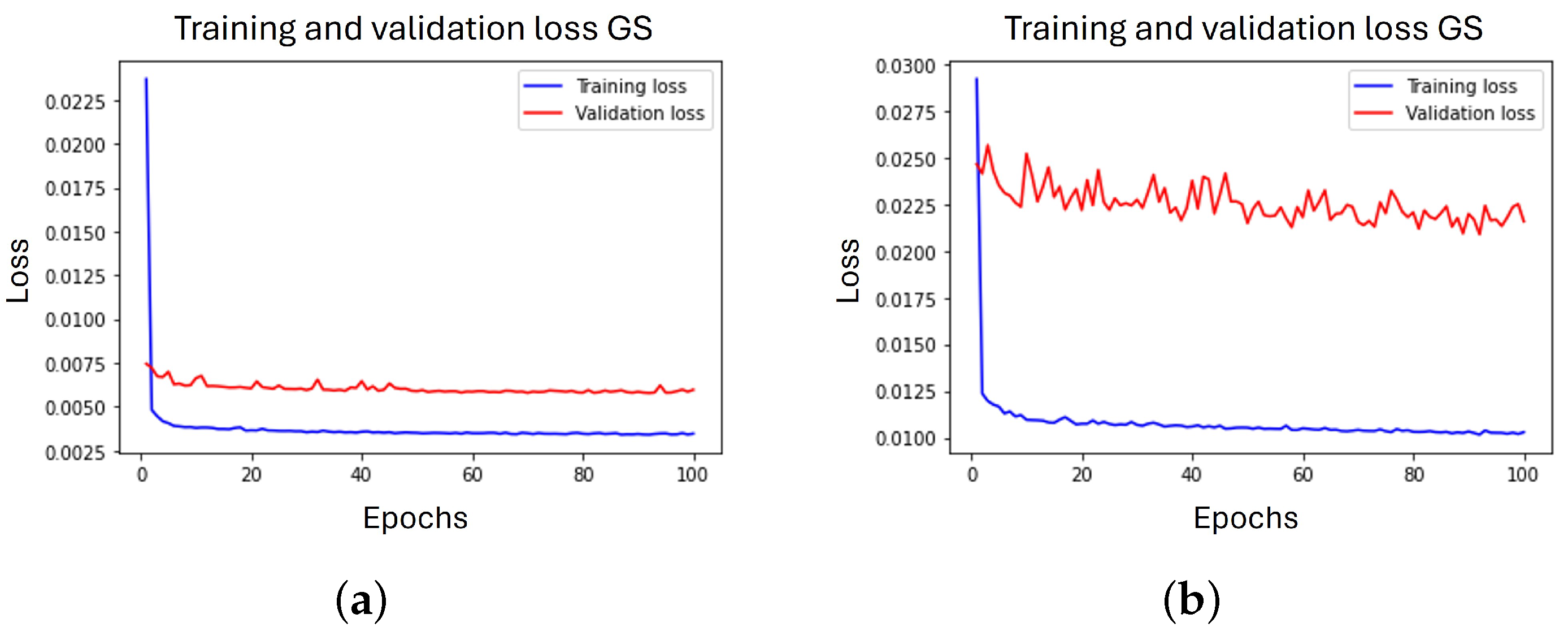
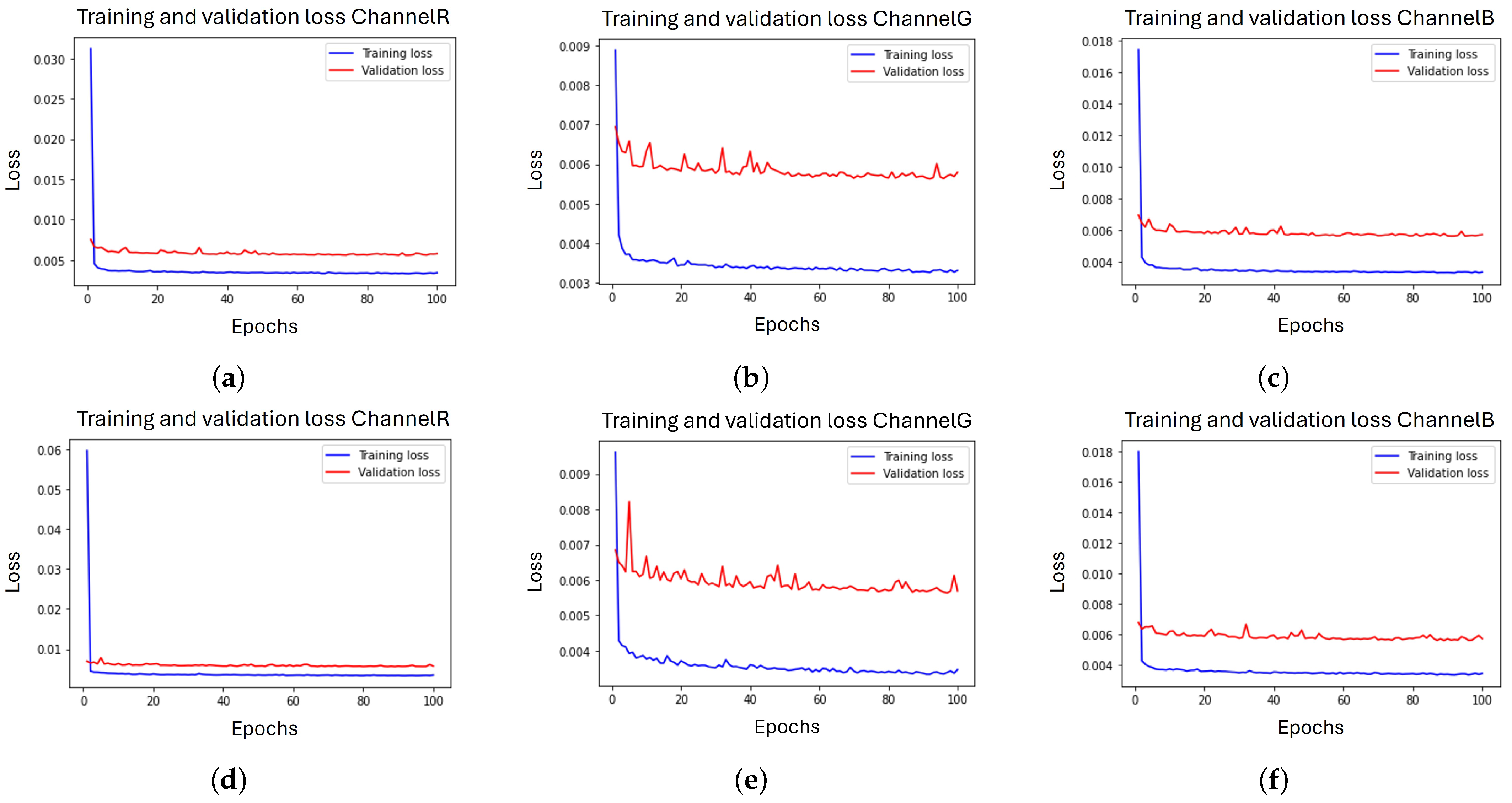
The learning curves obtained during the training process are illustrated in Figure 5 and Figure 6.

4. Experimental Results

It is essential to recognize that all algorithms require a validation process to assess their effectiveness in comparison to existing methods. To gain a comprehensive understanding of their performance, it is crucial to employ techniques that quantitatively and/or qualitatively evaluate their outcomes.

Therefore, the following quantitative and qualitative quality criteria were used to assess and validate the results obtained by DVACE in comparison to the other specialized techniques discussed in Section 2.

Quantitative metrics provide a means of evaluating the quality of digital images after processing. These metrics can be categorized into reference-based metrics, which compare the processed image against a ground truth, and non-reference metrics, which assess image quality without requiring a reference. The metrics used in this study are as follows:

• Erreur Relative Globale Adimensionnelle de Synthèse (ERGAS) [22,24].
• Mean Square Error (MSE) [22].
• Normalized Color Difference (NCD) estimates the perceptual error between two color vectors by converting from the $RGB$ space to the CIELuv space. This conversion is necessary because human color perception cannot be accurately represented using the RGB model as it is a non-linear space [25]. The perceptual color error between the two color vectors is defined as the Euclidean distance between them, as given by Equation (32).

  $$\Delta E_{Luv}=\sqrt{{(\Delta L^{\ast })}^2+{(\Delta u^{\ast })}^2+{(\Delta v^{\ast })}^2},$$

  (32)

  where $\Delta E_{Luv}$ is the error, and $\Delta L^{\ast }$, $\Delta u^{\ast }$, and y $\Delta v^{\ast }$ are the difference between the components $L^{\ast }$, $u^{\ast }$, and $v^{\ast }$, respectively, between the two color vectors under consideration.
  Once $\Delta E_{Luv}$ was found for each one of the pixels of the images under consideration, the NCD was estimated according to Equation (33).

  $$NCD={\displaystyle \frac{{\sum }_{i=0}^{M-1}{\sum }_{j=0}^{N-1}∥\Delta E_{Luv}∥}{{\sum }_{i=0}^{M-1}{\sum }_{j=0}^{N-1}∥E_{Luv}^{\ast }∥}},$$

  (33)

  where $E_{Luv}^{\ast }=\sqrt{{\left(L^{\ast }\right)}^2+{\left(u^{\ast }\right)}^2+{\left(v^{\ast }\right)}^2}$ is the norm of magnitude of the vector of the pixel of the original image not corrupted in space $L^{\ast }{u}^{\ast }{v}^{\ast }$, and M and N are the dimensions of the image.
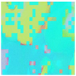
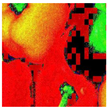
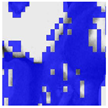
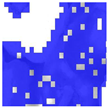
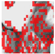
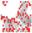
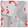
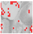
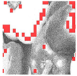
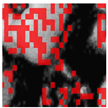
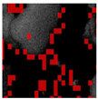
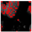
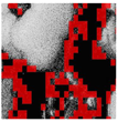
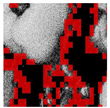
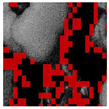
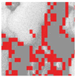
• Perception-based Image Quality Evaluator (PIQE) is a no-reference image quality assessment method that evaluates perceived image quality based on visible distortion levels [26]. Despite being a numerical metric, it is particularly useful for identifying regions of high activity, artifacts, and noise, as it generates masks that indicate the areas where these distortions occur. Consequently, PIQE is also classified as a qualitative metric as it is based on human perception and assesses visual quality from a non-mathematical perspective [26].
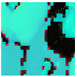
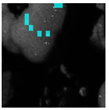
  The activity mask of an image is a tool that quantifies the level of detail or complexity in a specific region based on intensity variations. Its computation is derived from Equations (34) and (35).

  $$G(x,y)=\sqrt{G_x{(x,y)}^2+G_y{(x,y)}^2},$$

  (34)

  where $G(x,y)$ is the gradient of the image, and $G_x(x,y)$ y $G_x(x,y)$ are the derivatives of the image in the position $(x,y)$.

  $${\sigma }_{G_{B_i}}^2={\displaystyle \frac{1}{M^2}}\sum _{(x,y)\in B_i}{(G(x,y)-{\mu }_{G_{B_i}})}^2,$$

  (35)

  where ${\sigma }_{G_{B_i}}^2$ is the variance in each of the blocks, and the $B_i$ of size $MxM$ y ${\mu }_{G_{B_i}}$ is the average of the gradient in the block.
  The artifact mask in an image indicates distortions, such as irregular edges that degrade visual quality. These distortions are detected by analyzing non-natural patterns in regions with high activity levels, where inconsistent blocks are identified and classified as artifacts.
  The noise mask is evaluated based on variations in undesired activity within low-activity regions, measuring the dispersion of intensity values within a block, as shown in Equation (36). If the dispersion significantly exceeds the expected level, the region is classified as noise.

  $${\sigma }_{I_{B_i}}^2={\displaystyle \frac{1}{M^2}}\sum _{(x,y)\in Bi}{(I(x,y)-{\mu }_{I_{Bi}})}^2.$$

  (36)
• Peak Signal-to-Noise Ratio (PSNR) [22,27].
• Relative Average Spectral Error (RASE) [22,28].
• Root Mean Squared Error (RMSE) [22,29].
• Spectral Angle Mapper (SAM) [22,30].
• Structural Similarity Index (SSIM) [22,31].
• Universal Quality Image Index (UQI) [22,32].

The DVACE evaluation was performed using classic benchmark images commonly used for algorithm assessment, including Airplane, Baboon, Barbara, Cablecar, Goldhill, Lenna, Mondrian, and Peppers, in both RGB and GS formats. Each evaluation image was corrupted with Gaussian noise, with a variance ${\sigma }^2$ of $0.01$ and a mean intensity $\overline{x}$ ranging from $-0.5$ to $0.5$, in increments of $0.01$. 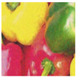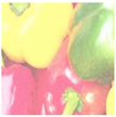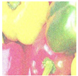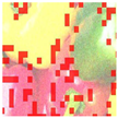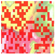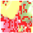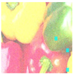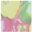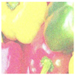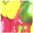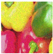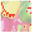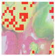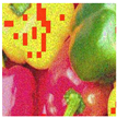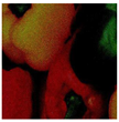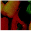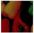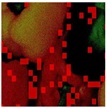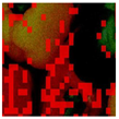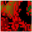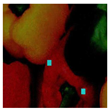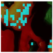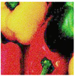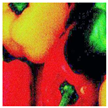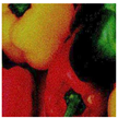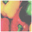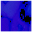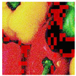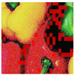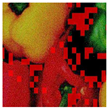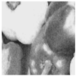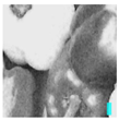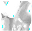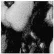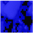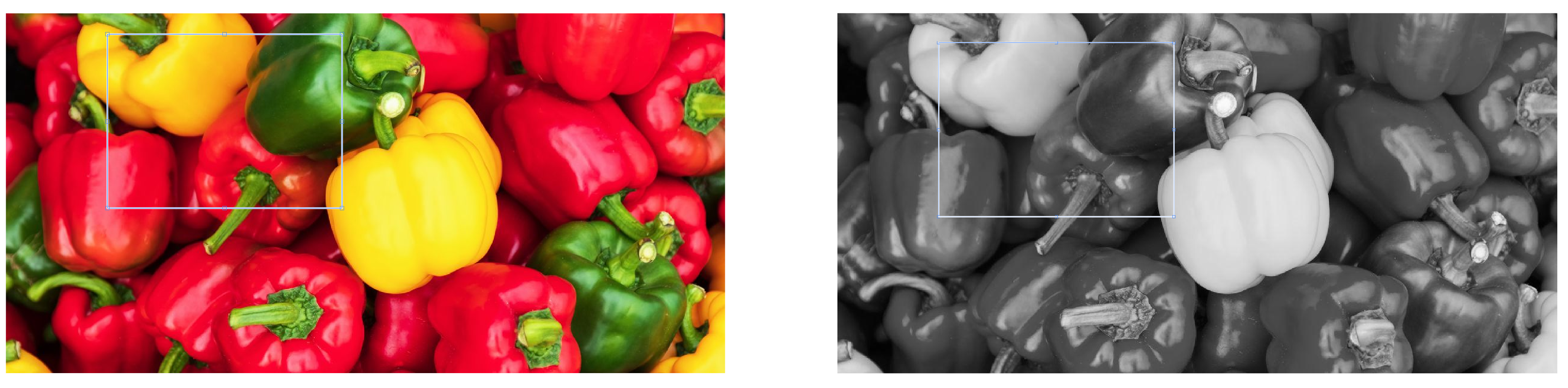Figure 7 presents a close-up of the original peppers in both RGB and GS formats.

As shown in

Table 2. Quantitative results for the peppers image in RGB with $\overline{x}=0.5$.

Image	SSIM	NCD	MSE	PSNR	RMSE	UQI	ERGAS	RASE	SAM
Noisy	0.536	0.889	11,911	7.371	109.137	0.455	25,525	3701	0.457
DVACE	0.832	0.402	1807	15.562	42.507	0.639	16,473	2371	0.271
Median	0.561	0.883	11,822	7.404	108.728	0.454	25,349	3676	0.453
DnCNN	0.556	0.877	11,741	7.434	108.354	0.456	25,349	3676	0.454
Nafnet	0.555	0.878	12,043	7.323	109.743	0.454	25,433	3688	0.460
Restormer	0.519	0.891	11,915	7.370	109.158	0.455	25,644	3718	0.461
SSR	0.418	0.924	13,238	6.913	115.057	0.455	26,482	3837	0.497
MSR	0.369	0.881	11,398	7.562	106.762	0.471	26,347	3815	0.499
MSRCP	0.529	0.888	11,864	7.389	108.920	0.455	25,557	3706	0.459
MSRCR	0.403	0.904	9670	8.277	98.336	0.482	25,628	3708	0.476
Gamma	0.708	0.664	4952	11.183	70.374	0.533	21,196	3059	0.327
Histogram	0.758	0.514	2538	14.086	50.379	0.610	19,432	2792	0.300

and

Table 3. Quantitative results for the peppers image in RGB with $\overline{x}=-0.5$.

Image	SSIM	NCD	MSE	PSNR	RMSE	UQI	ERGAS	RASE	SAM
Noisy	0.333	0.839	7144	9.592	84.519	0.195	1,349,244	inf	0.602
DVACE	0.807	0.287	998	18.139	31.592	0.721	21,449	3021	0.324
Median	0.332	0.842	7176	9.572	84.714	0.194	1,288,543	inf	0.545
DnCNN	0.339	0.842	7070	9.637	84.083	0.211	1,058,213	inf	0.494
Nafnet	0.351	0.843	6929	9.724	83.240	0.240	299,241	38,845	0.592
Restormer	0.344	0.834	6913	9.734	83.143	0.232	1,145,639	inf	0.585
SSR	0.741	0.273	1504	16.358	38.782	0.646	46,223	6526	0.413
MSR	0.741	0.279	1497	16.377	38.696	0.656	34,834	4939	0.407
MSRCP	0.742	0.436	2007	15.104	44.805	0.507	376,226	inf	0.563
MSRCR	0.761	0.237	1166	17.462	34.154	0.653	49,323	7324	0.388
Gamma	0.635	0.580	2931	13.461	54.134	0.505	453,785	inf	0.433
Histogram	0.603	0.389	4337	11.759	65.857	0.591	20,978	3049	0.438

, the quantitative results for the peppers RGB image are presented for $\overline{x}=0.5$ and $\overline{x}=-0.5$, respectively, with ${\sigma }^2=0.1$. It is evident that, in most cases where the mean was nonzero, DVACE achieved superior image restoration.

Similarly,

Table 4. Quantitative results for the peppers image in GS with $\overline{x}=0.5$.

Image	SSIM	NCD	MSE	PSNR	RMSE	UQI	ERGAS	RASE	SAM
Noisy	0.286	2.685	13,567	6.806	116.475	0.528	14,248	3562	0.381
DVACE	0.714	0.935	2526	14.107	50.256	0.792	9400	2350	0.186
Median	0.458	2.681	13,395	6.861	115.736	0.528	14,095	3524	0.371
DnCNN	0.584	2.633	13,122	6.951	114.551	0.532	14,013	3503	0.370
Nafnet	0.576	2.732	13,840	6.720	117.642	0.524	14,142	3536	0.378
Restormer	0.276	2.663	13,440	6.847	115.930	0.530	14,245	3561	0.381
SSR	0.236	2.541	13,860	6.713	117.729	0.533	13,902	3476	0.433
MSR	0.282	1.842	9793	8.221	98.962	0.588	12,751	3188	0.434
MSRCP	0.282	2.667	13,471	6.837	116.067	0.529	14,226	3556	0.381
MSRCR	0.282	1.846	9821	8.209	99.099	0.587	12,758	3189	0.435
Gamma	0.252	1.942	8107	9.042	90.037	0.616	13,416	3354	0.308
Histogram	0.207	1.018	3123	13.185	55.886	0.816	12,986	3247	0.278

and

Table 5. Quantitative results for the peppers image in GS with $\overline{x}=-0.5$.

Image	SSIM	NCD	MSE	PSNR	RMSE	UQI	ERGAS	RASE	SAM
Noisy	0.039	0.912	8,630	8.771	92.896	0.086	2,489,114	inf	0.706
DVACE	0.538	0.329	1673	15.897	40.899	0.560	61,802	15,450	0.330
Median	0.085	0.926	8679	8.746	93.159	0.082	2,451,183	inf	0.654
DnCNN	0.145	0.925	8456	8.859	91.954	0.087	1,877,656	inf	0.607
Nafnet	0.162	0.917	8138	9.026	90.208	0.099	781,272	inf	0.580
Restormer	0.040	0.909	8543	8.815	92.427	0.089	1,708,935	inf	0.701
SSR	0.136	0.435	3150	13.147	56.129	0.449	126,333	31,583	0.500
MSR	0.183	0.429	2859	13.568	53.473	0.500	67,115	16,779	0.474
MSRCP	0.068	0.484	3480	12.715	58.993	0.415	268,579	inf	0.528
MSRCR	0.075	0.448	3606	12.561	60.049	0.383	417,730	inf	0.538
Gamma	0.076	0.698	5059	11.090	71.129	0.256	562,233	inf	0.565
Histogram	0.391	1.254	5544	10.692	74.459	0.680	11,327	2832	0.345

present the quantitative results for the peppers GS image for different mean values and ${\sigma }^2=0.1$. It was observed that, in most cases where $\overline{x}\ne 0$, DVACE achieved superior image restoration compared to all the other algorithms used for comparison.

As shown in Table 4 and Table 5, the peppers image was evaluated under different noise conditions. DVACE consistently achieves the highest SSIM and PSNR, with the lowest MSE, RMSE, and NCD, ensuring optimal noise reduction and contrast enhancement. It also minimized ERGAS, RASE, and SAM, confirming its superior spectral fidelity. Histogram Equalization and Gamma Correction improved contrast but introduced spectral distortions. The deep learning-based methods (DnCNN, NafNet, and Restormer) showed variability, while the MSR-based techniques and SSR exhibited higher error rates. DVACE maintained the best trade-off between denoising and structural fidelity.

Table 6. Qualitative results for the peppers image in RGB.

Feature	Noisy Image	DVACE	Median	DnCNN	NAFNet	Restormer
$\overline{x}=0.5$
Activity mask
Artifact mask
Noise Mask
Feature	SSR	MSR	MSRCP	MSRCR	Gamma	Histogram Eq.
$\overline{x}=-0.5$
Activity Mask
Artifact Mask
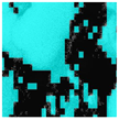
Noise Mask

presents a visual comparison of the results obtained by DVACE and the aforementioned algorithms for both noise reduction and contrast enhancement on the baboon image in RGB with $\overline{x}=0.5$. This table illustrates that, while the proposed algorithm introduces some distortions, it achieves the best noise reduction results alongside the NAFNet network. Additionally, in terms of contrast enhancement, DVACE demonstrated superior restoration (comparable to Histogram Equalization).

Table 7. Qualitative results for the peppers image in RGB.

Feature	Noisy Image	DVACE	Median	DnCNN	NAFNet	Restormer
$\overline{x}=-0.5$
Activity Mask
Artifact Mask
Noise Mask
Feature	SSR	MSR	MSRCP	MSRCR	Gamma	Histogram Eq.
$\overline{x}=-0.5$
Activity Mask
Artifact Mask
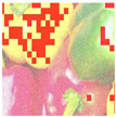
Noise Mask

presents a visual comparison for the peppers image in RGB with $\overline{x}=-0.5$. Visually, DVACE and the median filter exhibited less noise reduction. However, the contrast enhancement achieved by DVACE was comparable to that of the dedicated algorithms designed for this task.

Table 8. Qualitative results for the peppers image in GS.

Feature	Noisy Image	DVACE	Median	DnCNN	NAFNet	Restormer
$\overline{x}=0.5$
Activity Mask
Artifact Mask
Noise Mask
Feature	SSR	MSR	MSRCP	MSRCR	Gamma	Histogram Eq.
$\overline{x}=-0.5$
Activity Mask
Artifact Mask
Noise Mask

presents a comparison for the peppers image in GS with $\overline{x}=0.5$. The results indicate that DVACE achieved the best performance in both noise reduction and contrast enhancement.

Table 9. Qualitative results for the peppers image in GS.

Feature	Noisy Image	DVACE	Median	DnCNN	NAFNet	Restormer
$\overline{x}=-0.5$
Activity Mask
Artifact Mask
Noise Mask
Feature	SSR	MSR	MSRCP	MSRCR	Gamma	Histogram Eq.
$\overline{x}=-0.5$
Activity Mask
Artifact Mask
Noise Mask

presents a comparison for the peppers GS image with $\overline{x}=-0.5$, confirming the trend observed with DVACE, which achieved the best results in both noise reduction and contrast enhancement.

As such, in general, Table 6, Table 7, Table 8 and Table 9 provide a visual assessment of DVACE against alternative methods. DVACE, DnCNN, and NAFNet produced cleaner images with well-preserved details, while Histogram Equalization and Gamma Correction enhanced contrast but amplified artifacts. Activity masks show DVACE retained details with minimal distortions. Artifact masks reveal that DVACE introduced fewer distortions than Median and MSRCP, while noise masks confirmed superior noise suppression compared to MSR-based methods and SSR. Overall, DVACE provided the most balanced restoration.

To comprehensively present the results of the metrics calculated from the images in the validation dataset, which were processed by each of the aforementioned methods, box plots are provided below. Figure 8 presents the ERGAS metric distribution across different methods. The noisy image showed the highest values, with DVACE achieving a low median and minimal variance, confirming its stable performance. Histogram Equalization and Gamma Correction also performed well, whereas MSR and MSRCR exhibited higher ERGAS values, indicating weaker global reconstruction. DVACE maintained a consistent advantage with fewer outliers.

Figure 9 illustrates the MSE distribution. The noisy image exhibits high error and dispersion, while DVACE achieved a lower median MSE with reduced variance, ensuring effective reconstruction. The deep learning models (DnCNN and NafNet) showed greater variability, and the MSR-based methods performed inconsistently. DVACE remained one of the most reliable techniques.

Notably, Gamma Correction and Histogram Equalization, despite not being deep learning techniques or having noise reduction capabilities, achieved the next best results. In contrast, SSR demonstrated the poorest performance as both its dispersion and average error were significantly higher than those of the other methods.

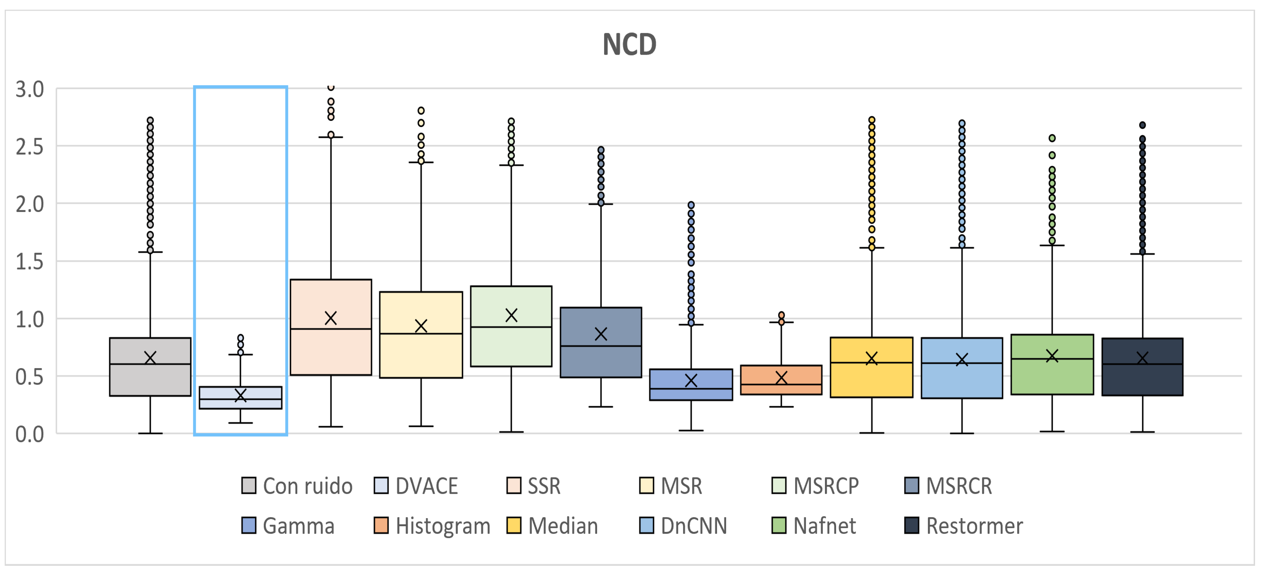
As shown in Figure 10, the NCD metric, which reflects color fidelity, was evaluated. DVACE achieved one of the lowest median NCD values with minimal dispersion, confirming its effectiveness in preserving perceptual color accuracy. While Histogram Equalization and Gamma Correction yielded competitive results, it introduce variability. The deep learning methods performed well but with slightly higher dispersion.

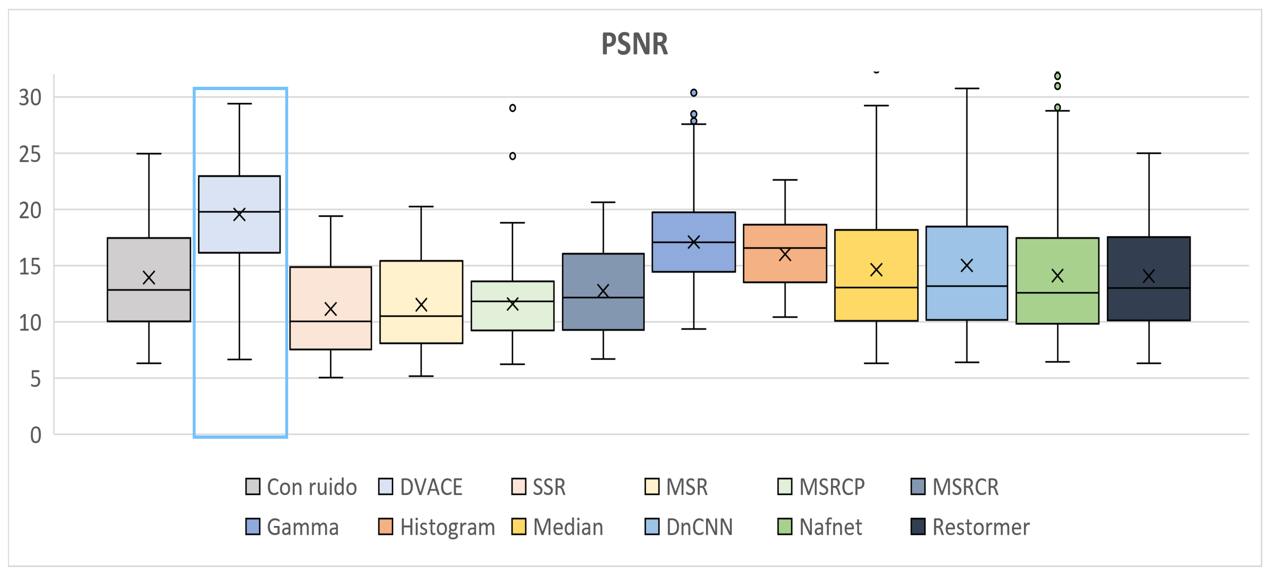
Figure 11 presents the PSNR distribution. The noisy image exhibited the lowest values, while DVACE achieved a high median PSNR with low variance, ensuring effective noise reduction and image fidelity. The deep learning models maintained competitive values but showed dataset-dependent behavior. The MSR-based methods performed worse in key metrics.

As shown in Figure 12, the RASE values, which indicate spectral reconstruction accuracy, were captured. The noisy image had the highest values, whereas DVACE maintained a lower median with reduced variance. Histogram Equalization and Gamma Correction achieved good results but exhibited more variability. The deep learning models and MSR-based methods showed inconsistent performance.

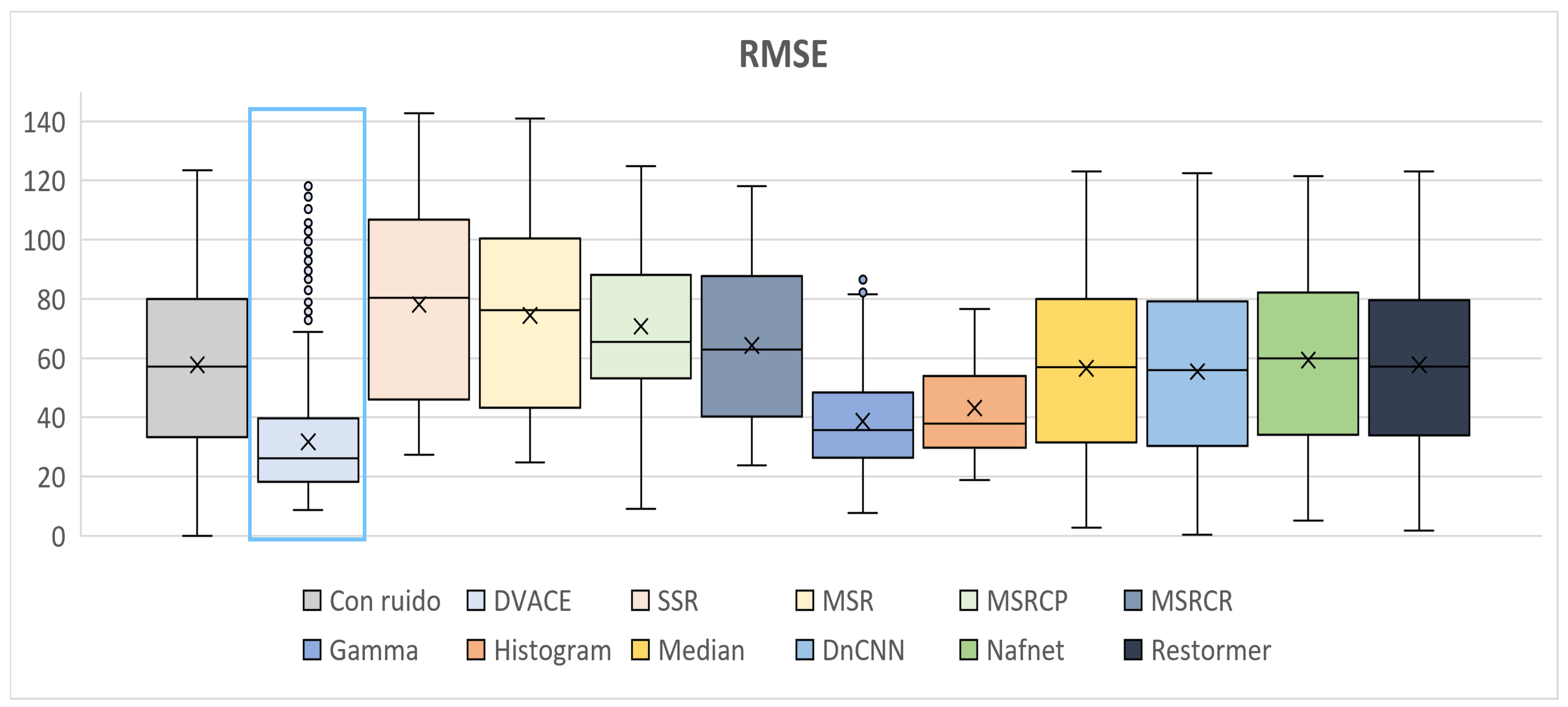
Figure 13 illustrates the RMSE values, reflecting the reconstruction accuracy. The noisy image exhibited the highest RMSE, while DVACE achieved a low median with reduced dispersion, confirming its stability. The deep learning models remained competitive but more variable. The MSR-based methods and SSR showed weaker performance.

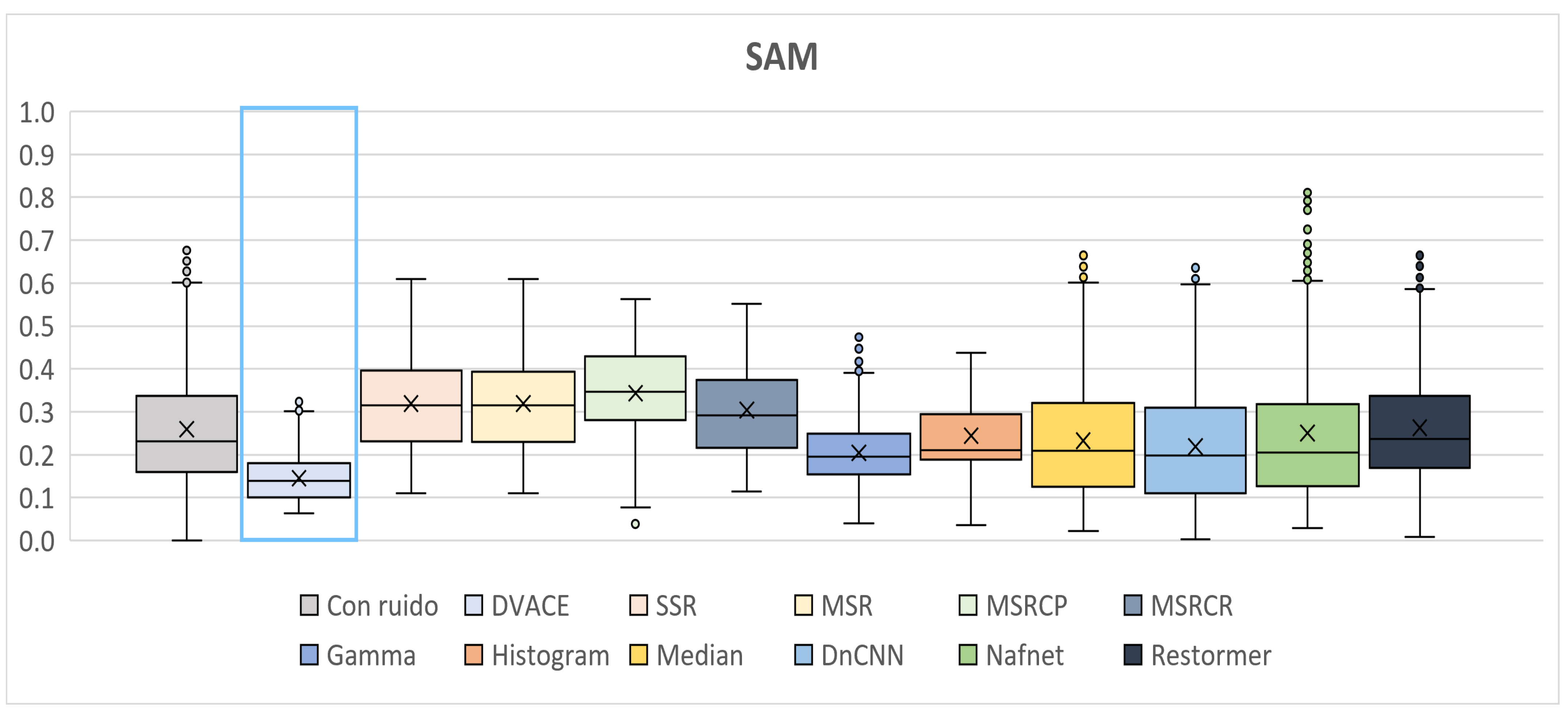
Figure 14 presents the SAM values, which measure the spectral fidelity. The noisy image showed significant spectral distortions, while DVACE achieved one of the lowest median SAM values, ensuring improved spectral consistency. Histogram Equalization and Gamma Correction performed well but introduced more variability.

As shown in Figure 15, the SSIM, which reflects the image quality, was evaluated. The noisy image had the lowest values, while DVACE achieved a high median with minimal variance, confirming its structural preservation. The deep learning models showed competitive performance, while the MSR-based methods underperformed.

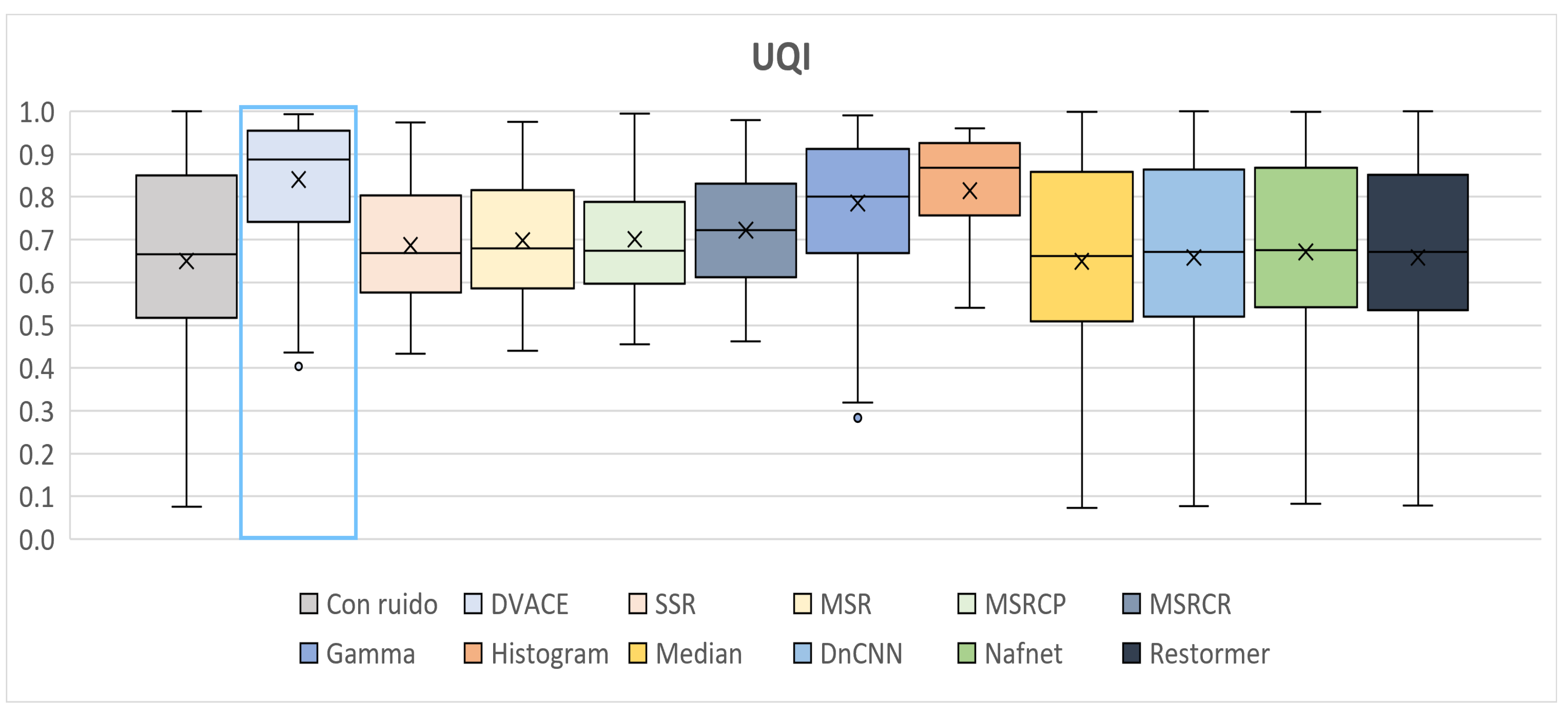
Finally, as shown in Figure 16, the UQI values, which assess the perceptual quality, were recorded. The noisy image exhibited the lowest UQI, while DVACE achieved one of the highest medians with low dispersion, ensuring strong consistency. The deep learning models performed well but exhibited slightly higher variability.

Another critical factor to consider when evaluating the effectiveness of an image restoration method is its execution speed.

Table 10. The average processing time for different images sizes, noise density, and image type.

Size	100 × 100	200 × 200	400 × 400	800 × 800	1600 × 1600	3200 × 3200
RGB	0.029 s	0.032 s	0.044 s	0.058 s	0.115 s	0.292 s
GS	0.085 s	0.098 s	0.140 s	0.183 s	0.342 s	0.964 s

presents the execution times of DVACE for images with dimensions $100\times 100$, $200\times 200$, $400\times 400$, $800\times 800$, $1600\times 1600$, and $3200\times 3200$, all of which were corrupted via Gaussian noise with ${\sigma }^2=0.01$ and $\overline{x}\in [-0.5, 0.5]$.

Table 11. Comparison of the processing time between DVACE and DnCNN of the images in GS.

Methods	DnCNN-S	DnCNN-B	DVACE
256 × 256	0.014 s	0.016 s	0.038 s
512 × 512	0.051 s	0.060 s	0.049 s
1024 × 1024	0.200 s	0.235 s	0.075 s

compares DVACE with two versions of DnCNN, showing that DVACE maintained competitive execution times, especially for larger image resolutions. For 512 × 512 and 1024 × 1024, DVACE outperformed DnCNN in efficiency, with processing times of 0.049 s and 0.075 s, respectively, demonstrating its advantage in speed without compromising restoration quality.

5. Conclusions

This research highlights the importance of proper image processing in addressing two distinct yet simultaneous challenges that can arise during image capture: poor lighting and noise. Based on this, a methodology is proposed using an autoencoder capable of processing images of any size and type (RGB or GS) under noisy and low-light conditions.

When analyzing the results presented, it was observed that DVACE effectively reduces Gaussian noise in images and enhances their contrast through deep learning techniques implemented in the proposed algorithm, regardless of the average noise level in the degraded images. The results of DVACE, both visually and across various quantitative metrics, demonstrate superior noise reduction and contrast enhancement compared to classical and deep learning-based specialized techniques.

One limitation observed in this research was that DVACE introduces distortions and reduces image activity. Therefore, we recommend using DVACE as a foundation for further improvements (such as integrating a sharpness enhancement algorithm to mitigate distortions and increase image activity).