Multivariate Modified Dugum Distribution and Its Applications

Abstract

The modified Dagum distribution is a highly versatile statistical model, and it is included in several important parametric families of distributions, with applications, such as economics and public health. In this paper, we introduce a multivariate version of the modified Dagum distribution and deduce some of its sub-models to address specific analytical needs. We use two different approaches to derive the joint probability density function for the proposed distribution. Also, we derive the joint cumulative distribution function through the traditional method and the Clayton copula methods. In addition, we explore and discuss some statistical properties, including the multivariate dependence. Further, we use the maximum likelihood method to estimate the unknown parameters and the associated confidence interval. Finally, we apply the proposed model to analyze some real data sets, including a protein consumption data set and a warranty policy data set, for demonstrative purposes. The marginals of the proposed model fit the data sets quite well, and the results demonstrate the model’s effectiveness in modeling the proposed data.

1. Introduction

The IWD is a versatile tool that can be easily applied to model various processes across different fields. These include reliability, ecology, medicine, biological studies, public health, and economics. The distribution has been extensively explored in the literature, where its properties and wide-ranging applications have been discussed. Notable contributions can be found in the works of [1,2,3,4].

The CDF and PDF of the IWD with parameters $(\lambda ,\alpha )$ is given, respectively, by

$$\begin{array}{c}\hfill G(x;\lambda ,\alpha )=e^{{\displaystyle \frac{-1}{\lambda x^{\alpha }}}},x>0,\end{array}$$

(1)

and

$$\begin{array}{c}\hfill g(x;\lambda ,\alpha )={\displaystyle \frac{\alpha }{\lambda }}{\left({\displaystyle \frac{1}{x}}\right)}^{\alpha +1}{e}^{{\displaystyle \frac{-1}{\lambda x^{\alpha }}}},x>0,\end{array}$$

(2)

where $\lambda >0$ is the scale parameter and $\alpha >0$ is the shape parameter.

The GIWD was first introduced by [5] and has proven to be an effective model for a wide range of applications. It is particularly useful in fields such as medicine and biological studies, where it can accurately represent various processes. Its flexibility makes it a valuable tool in these disciplines, providing a reliable framework for modeling complex phenomena.

The CDF and PDF of the GIWD with parameters $(\lambda ,\alpha ,\xi )$ are given, respectively, by

$$\begin{array}{c}\hfill G(x;\lambda ,\alpha ,\xi )=e^{{\displaystyle \frac{-\xi }{\lambda x^{\alpha }}}},x>0,\end{array}$$

(3)

and

$$\begin{array}{c}\hfill g(x;\lambda ,\alpha ,\xi )={\displaystyle \frac{\alpha \xi }{\lambda }}{\left({\displaystyle \frac{1}{x}}\right)}^{\alpha +1}{e}^{{\displaystyle \frac{-\xi }{\lambda x^{\alpha }}}},x>0,\end{array}$$

(4)

where $\lambda >0$ and $\xi >0$ are the scale parameters and $\alpha >0$ is the shape parameter.

The authors of [6] successfully defined the three-parameter modified Weibull distribution by extending the traditional Weibull distribution. This extension involved the inclusion of an additional term, $e^{-\gamma x}$. Similarly, the authors of [7] developed a new extended Weibull distribution by modifying the Weibull distribution through the addition of the term $e^{{\displaystyle \frac{-\gamma }{x}}}$. Following a comparable approach, it is possible to derive the MGIWD by adding the term $e^{-\gamma x}$. Then, the CDF and PDF of the MGIWD with parameters $(\lambda ,\alpha ,\xi ,\gamma )$ can be given, respectively, as

$$\begin{array}{c}\hfill G(x;\lambda ,\alpha ,\xi ,\gamma )=e^{{\displaystyle \frac{-\xi }{\lambda x^{\alpha }}}{e}^{-\gamma x}},x>0,\end{array}$$

(5)

and

$$\begin{array}{c}\hfill g(x;\lambda ,\alpha ,\xi ,\gamma )={\displaystyle \frac{\xi }{\lambda }}{\left({\displaystyle \frac{1}{x}}\right)}^{\alpha +1}(\gamma x+\alpha )e^{-\gamma x}{e}^{{\displaystyle \frac{-\xi }{\lambda x^{\alpha }}}{e}^{-\gamma x}},x>0,\end{array}$$

(6)

where $\lambda >0$ and $\xi >0$ are the scale parameters and $\alpha >0$ and $\gamma \ge 0$ are the shape parameters.

The DD, which was first proposed by [8], has found several important applications across a variety of fields. In finance, actuarial sciences, and economics, it plays a key role in modeling the distribution of personal income, where it is highly valued for its ability to represent income size distribution. The DD, which is the most well-known model in economics, is essentially a BIIID with an added scale parameter and a sub-model of the GB2, as highlighted by [9].

The CDF and PDF of DD with parameters $(b,a,\varphi )$ are given, respectively, as

$$\begin{array}{c}\hfill W(x;b,a,\varphi )={\displaystyle \frac{1}{{\left(1+b{x}^{-a}\right)}^{\varphi }}},x>0,\end{array}$$

(7)

and

$$\begin{array}{c}\hfill w(x;b,a,\varphi )={\displaystyle \frac{b\varphi a{x}^{-a-1}}{{\left(1+b{x}^{-a}\right)}^{\varphi +1}}},x>0,\end{array}$$

(8)

where $b>0$ is a scale parameter and $a>0$ and $\varphi >0$ are the shape parameters.

A generalization for DD has been proposed by a number of authors in order to produce more adaptable models. The authors of [10] presented a new model named gamma Dagum distribution, and the Weibull Dagum distribution was proposed by [11]. By explicitly interpreting the Dagum family’s parameters in terms of the income median, inequality, and poverty measures, ref. [12] proposed novel formulations of the Dagum family, which are widely appreciated for modeling the income distribution. In [13], the exponentiated generalized exponential Dagum distribution was proposed and investigated. One of the generalizations that is the subject of this study is the MDD, which was studied by [14]. It is also considered a generalization of both MBIIID [15] and the modified Fr´echet distribution [16]. The CDF and PDF of MDD with parameters $(b,a,\varphi ,c)$ can be written, respectively, as

$$\begin{array}{c}\hfill W(x;b,a,\varphi ,c)={\displaystyle \frac{1}{{\left(1+b{x}^{-a}{e}^{-cx}\right)}^{\varphi }}},x>0,\end{array}$$

(9)

and

$$\begin{array}{c}\hfill w(x;b,a,\varphi ,c)={\displaystyle \frac{b\varphi e^{-cx}{x}^{-a-1}(cx+a)}{{\left(1+b{x}^{-a}{e}^{-cx}\right)}^{\varphi +1}}},x>0,\end{array}$$

(10)

where $b>0$ is a scale parameter and $a>0$, $c>0$, and $\varphi >0$ are the shape parameters.

A range of CDF forms that can be useful for fitting data was outlined by [17]. These forms provide different approaches for modeling and analyzing data in various contexts. Among the various CDFs discussed, one notable example is the BIIID, which is often employed due to its versatility and ability to fit different types of data effectively. The BIIID has a wide range of applications in statistical modeling. It is particularly useful in various fields where statistical analysis is essential, including reliability, forestry, and engineering; see, for example, [18,19,20]. The CDF and PDF of BIIID with parameters $(a,\varphi )$, which are a special case of the CDF and PDF for DD when $b=1$ in Equations (7) and (8), can be written, respectively, as

$$\begin{array}{c}\hfill W(x;a,\varphi )={\displaystyle \frac{1}{{\left(1+{\left(\frac{1}{x}\right)}^a\right)}^{\varphi }}},x>0,\end{array}$$

(11)

and

$$\begin{array}{c}\hfill w(x;a,\varphi )={\displaystyle \frac{a\varphi }{x^{a+1}{\left(1+{\left(\frac{1}{x}\right)}^a\right)}^{\varphi +1}}},x>0.\end{array}$$

(12)

There are various techniques available for introducing multivariate distributions. One of the earliest approaches was proposed by [21], who introduced the multivariate Pareto distribution. This particular distribution is characterized by having Pareto marginals, which are individual Pareto distributions for each variable in the multivariate context. Another technique for obtaining multivariate distributions is introduced by [22]. In his paper, a method to derive the multivariate Burr Type-XII distribution is presented. This distribution is notable for deriving Burr Type-XII marginals, meaning that each individual marginal follows a Burr Type-XII distribution. Additionally, ref. [23] proposed a new class of multivariate distributions conducted by compounding the likelihood function of a specific distribution with a gamma distribution. Also, by applying a suitable transformation to Takahashi’s multivariate Burr distribution [22], ref. [24] introduce a new type of distribution known as the MVGED. Ref. [25] introduces two distinct techniques for creating multivariate versions of the GB2 distribution. The first technique emphasizes stochastic dependency through gamma random variables, while the second relies on generalizing the distribution of the order statistics.

Copulas are powerful multivariate statistical modeling tools that depict the dependence structure between random variables independently of their marginal distributions. According to Sklar’s Theorem (see [26]), each multivariate distribution can be decomposed into its marginal distributions and an associated copula function. Also, the concept of a copula is derived from the separation of the joint CDF into two parts: one that explains the dependent structure and the other that describes the marginal behavior. Among the various families of copulas, the Clayton copula is widely used for modeling asymmetric lower tail dependence. Let the k-variate random vector $\Omega ={\Omega }_1,\dots ,{\Omega }_k$; then, the k-variate Clayton copula can be given as

$$\begin{array}{c}\hfill C_{\theta }({\omega }_1,\dots ,{\omega }_k)={\displaystyle \frac{1}{{({\omega }_1^{-1/\theta }+\dots +{\omega }_k^{-1/\theta }-(k-1))}^{\theta }}},\end{array}$$

(13)

where ${\omega }_1,\dots ,{\omega }_k\in [0,1]$ are uniformly distributed marginal variables, and $\theta >0$ is the copula parameter controlling the strength of dependence. As $\theta \to 0$, the Clayton copula approaches independence.

This paper uses two methods suggested in [21,22] to obtain the joint PDF for the MVMDD and its sub-models. Furthermore, it is possible to demonstrate that the joint CDF for MVMDD can be achieved for the first approach by using the conventional approach, and the second approach can be obtained by using the Clayton copula. Several properties are discussed for MVMDD. The maximum likelihood estimation cannot be obtained in closed form, so a numerical method can be used. The effectiveness of the suggested model and the approach in a practical setting has been demonstrated using two real data sets.

The structure of the paper is organized as follows. Section 2 presents the derivation of some necessary prerequisites. In Section 3, the MVMDD and its sub-models are introduced. Section 4 explores various statistical properties of these distributions. Section 5 investigates the multivariate dependence properties for MVMDD. The maximum likelihood estimation method is discussed in Section 6. Two applications within the public health field and warranty policies are illustrated in Section 7. Finally, Section 8 provides concluding remarks and future work.

2. Prerequisites

In this section, the PDF of MDD can be obtained by another approach using the methodology proposed by [22] as follows:

Suppose $\lambda >0$ is a random variable with an inverse gamma distribution with PDF; $u(\lambda ;\theta ,\beta )$ is provided by

$$\begin{array}{c}\hfill u(\lambda ;\theta ,\beta )={\displaystyle \frac{{\beta }^{\theta }}{\Gamma \left(\theta \right)}}{\left({\displaystyle \frac{1}{\lambda }}\right)}^{\theta +1}{e}^{{\displaystyle \frac{-\beta }{\lambda }}},\lambda >0,\end{array}$$

(14)

using the methodology suggested by [22], the PDF of the MDD can be given by MGIWD (6) with inverse gamma distribution (14) as compounded as

$$\begin{array}{cc}\hfill f(x;\theta ,\beta ,\alpha ,\gamma )& ={\int }_{-\infty }^{+\infty }u(\lambda ;\theta ,\beta )g(x;\lambda ,\alpha ,\xi ,\gamma )d\lambda \hfill \\ & ={\int }_0^{\infty }{\displaystyle \frac{{\beta }^{\theta }}{\Gamma \left(\theta \right)}}{\left({\displaystyle \frac{1}{\lambda }}\right)}^{\theta +1}{e}^{{\displaystyle \frac{-\beta }{\lambda }}}{\displaystyle \frac{\xi }{\lambda }}{\left({\displaystyle \frac{1}{x}}\right)}^{\alpha +1}(\gamma x+\alpha )e^{-\gamma x}{e}^{{\displaystyle \frac{-\xi }{\lambda x^{\alpha }}}{e}^{-\gamma x}}d\lambda \hfill \\ & =(\alpha +\gamma x)\xi e^{-\gamma x}{\displaystyle \frac{{\beta }^{\theta }}{\Gamma \left(\theta \right)}}{\left({\displaystyle \frac{1}{x}}\right)}^{\alpha +1}{\int }_0^{\infty }{\left({\displaystyle \frac{1}{\lambda }}\right)}^{\theta +2}{e}^{{\displaystyle \frac{-1}{\lambda }}(\beta +\xi x^{-\alpha }{e}^{-\gamma x})}d\lambda \hfill \\ & =(\alpha +\gamma x)\xi e^{-\gamma x}{\displaystyle \frac{{\beta }^{\theta }}{\Gamma \left(\theta \right)}}{\left({\displaystyle \frac{1}{x}}\right)}^{\alpha +1}{\displaystyle \frac{\Gamma (1+\theta )}{{\left(\beta +\xi x^{-\alpha }{e}^{-\gamma x}\right)}^{\theta +1}}}\hfill \\ & =(\alpha +\gamma x)\xi \theta e^{-\gamma x}{\beta }^{\theta }{\left({\displaystyle \frac{1}{x}}\right)}^{\alpha +1}{\displaystyle \frac{1}{{\left(\beta +\xi x^{-\alpha }{e}^{-\gamma x}\right)}^{\theta +1}}}.\hfill \end{array}$$

(15)

The PDF for MDD, which is given by (10), can be obtained from (15) by putting $\xi =b$, $\theta =\varphi$, $\gamma =c$, $\alpha =a$, and $\beta =1$.

3. Multivariate Modified Dagum Distribution

In this section, the joint PDF and the joint CDF of the MVMDD can be derived through two distinct approaches. Each approach offers a unique technique to calculate the joint PDF and the joint CDF, allowing for flexibility depending on the chosen technique. Utilizing both methods can lead to a deeper and more comprehensive understanding of the distribution’s behavior. Additionally, the joint survival function can also be derived.

3.1. Approach (1): The Joint PDF

Consider a multivariate modified generalized inverse Weibull distribution (MVMGIWD), where each marginal follows a generalized inverse Weibull distribution given by Equation (6). The joint density function of the MVMGIWD can be expressed as

$$\begin{array}{c}\hfill g(\mathit{x};\mathit{\alpha };\mathit{\xi };\mathit{\gamma },\lambda )=\prod _{i=1}^k\left({\xi }_i({\gamma }_i{x}_i+{\alpha }_i){\displaystyle \frac{1}{\lambda }}{\left({\displaystyle \frac{1}{x_i}}\right)}^{{\alpha }_i+1}{e}^{-\gamma x}{e}^{{\displaystyle \frac{-{\xi }_i{e}^{-{\gamma }_i{x}_i}}{\lambda x_i^{{\alpha }_i}}}}\right),\end{array}$$

(16)

where $\mathit{x}=(x_1,\dots ,x_k)$, $\mathit{\alpha }=({\alpha }_1,\dots ,{\alpha }_k)$, $\mathit{\xi }=({\xi }_1,\dots ,{\xi }_k)$, and $\mathit{\gamma }=({\gamma }_1,\dots ,{\gamma }_k)$. Following the technique described in [22], we integrate the joint PDF of MVMGIWD with regard to an inverse gamma mixing distribution. This yields the MVMDD, which captures dependencies between variables. This leads us to the following lemma, which formally presents the joint PDF of the MVMDD.

Lemma 1.

Assume that ${\alpha }_1$,…,${\alpha }_n\ge 1$, $\theta \ge 0$, ${\xi }_1$,…,${\xi }_n>0$ and ${\gamma }_1$,…,${\gamma }_n>0$. Consider $x_1,\dots ,x_n$ to have a multivariate MGIWD with joint PDF given by (16). Then, the joint PDF for MVMDD can be derived as

$$\begin{array}{c}\hfill f(\mathit{x};\mathit{\alpha };\mathit{\xi };\mathit{\gamma };\theta )={\displaystyle \frac{\Gamma (k+\theta )}{\Gamma \left(\theta \right)}}{\displaystyle \frac{e^{-{\sum }_{i=1}^k{\gamma }_i{x}_i}{\prod }_{i=1}^k{\xi }_i({\gamma }_i{x}_i+{\alpha }_i)x_i^{-{\alpha }_i-1}}{{\left(1+{\sum }_{i=1}^k{\xi }_i{x}_i^{-{\alpha }_i}{e}^{-{\gamma }_i{x}_i}\right)}^{k+\theta }}},x_i>0,i=0,1,\dots ,k.\end{array}$$

(17)

Proof. 

Similar to the method outlined in [22], the MVMDD can be derived by compounding the MGIWD, as defined in Equation (16), with an inverse gamma distribution, as defined in Equation (15). This approach integrates out the scale parameter to introduce flexibility and dependence across variables. The resulting joint PDF of the MVMDD is given as

$$\begin{array}{ccc}\hfill f(\mathit{x};\mathit{\alpha };\mathit{\xi };\mathit{\gamma };\theta )& =& {\int }_0^{\infty }\prod _{i=1}^k\left({\xi }_i({\gamma }_i{x}_i+{\alpha }_i){\displaystyle \frac{1}{\lambda }}{\left({\displaystyle \frac{1}{x_i}}\right)}^{{\alpha }_i+1}{e}^{-{\gamma }_i{x}_i}{e}^{{\displaystyle \frac{-{\xi }_i{e}^{-{\gamma }_i{x}_i}}{\lambda x_i^{{\alpha }_i}}}}\right)\hfill \\ & \times & {\displaystyle \frac{{\beta }^{\theta }}{\Gamma \left(\theta \right)}}{\left({\displaystyle \frac{1}{\lambda }}\right)}^{\theta +1}{e}^{{\displaystyle \frac{-\beta }{\lambda }}}d\lambda \hfill \\ & =& {\displaystyle \frac{{\beta }^{\theta }}{\Gamma \left(\theta \right)}}\prod _{i=1}^k\left({\xi }_i({\gamma }_i{x}_i+{\alpha }_i){\left({\displaystyle \frac{1}{x_i}}\right)}^{{\alpha }_i+1}{e}^{-{\gamma }_i{x}_i}\right)\hfill \\ & \times & {\int }_0^{\infty }{e}^{{\displaystyle \frac{-1}{\lambda }}\left(\beta +{\sum }_{i=1}^k{\displaystyle \frac{{\xi }_i{e}^{-{\gamma }_i{x}_i}}{x_i^{{\alpha }_i}}}\right)}{\left({\displaystyle \frac{1}{\lambda }}\right)}^{k+\theta +1}d\lambda \hfill \\ & =& \prod _{i=1}^k\left({\xi }_i({\gamma }_i{x}_i+{\alpha }_i)x_i^{-{\alpha }_i-1}{e}^{-{\gamma }_i{x}_i}\right){\displaystyle \frac{\frac{{\beta }^{\theta }}{\Gamma \left(\theta \right)}\Gamma (k+\theta )}{{\left(\beta +{\sum }_{i=1}^k{\xi }_i{x}_i^{-{\alpha }_i}{e}^{-{\gamma }_i{x}_i}\right)}^{k+\theta }}}.\hfill \end{array}$$

By setting $\beta =1$, (17) is easily obtained, which is the joint PDF of MVMDD. Also, some important sub-models can be obtained from Equation (17) as shown in Table 1. Further, the MVMBIIID can be considered as a multivariate of the MBIIID given in [15]. □

Table 1. The sub-models from the joint PDF of MVMDD given by (17).

Distribution	Parameters	Joint PDF
MVDD [25]	${\gamma }_1=0,\dots ,{\gamma }_k=0$	$f(\mathit{x};\mathit{\alpha };\mathit{\xi };\theta )={\displaystyle \frac{\Gamma (k+\theta )}{\Gamma \left(\theta \right)}}{\displaystyle \frac{{\prod }_{i=1}^k{\xi }_i{\alpha }_i{x}_i^{-{\alpha }_i-1}}{{\left(1+{\sum }_{i=1}^k{\xi }_i{x}_i^{-{\alpha }_i}\right)}^{k+\theta }}}$
MVMBIIID [New]	${\xi }_1=1,\dots ,{\xi }_k=1$	$f(\mathit{x};\mathit{\alpha };\mathit{\gamma };\theta )={\displaystyle \frac{\Gamma (k+\theta )}{\Gamma \left(\theta \right)}}{\displaystyle \frac{e^{-{\sum }_{i=1}^k{\gamma }_i{x}_i}{\prod }_{i=1}^k({\gamma }_i{x}_i+{\alpha }_i)x_i^{-{\alpha }_i-1}}{{\left(1+{\sum }_{i=1}^k{x}_i^{-{\alpha }_i}{e}^{-{\gamma }_i{x}_i}\right)}^{k+\theta }}}$
MVBIIID [27]	${\gamma }_1=0,\dots ,{\gamma }_k=0$	$f(\mathit{x};\mathit{\alpha };\theta )={\displaystyle \frac{\Gamma (k+\theta )}{\Gamma \left(\theta \right)}}{\displaystyle \frac{{\prod }_{i=1}^k{\alpha }_i{x}_i^{-{\alpha }_i-1}}{{\left(1+{\sum }_{i=1}^k{x}_i^{-{\alpha }_i}\right)}^{k+\theta }}}$
	${\xi }_1=1,\dots ,{\xi }_k=1$
MVLD [27,28]	${\alpha }_1=0,\dots ,{\alpha }_k=0$	$f(\mathit{x};\mathit{\gamma };\theta )={\displaystyle \frac{\Gamma (k+\theta )}{\Gamma \left(\theta \right)}}{\displaystyle \frac{e^{-{\sum }_{i=1}^k{\gamma }_i{x}_i}{\prod }_{i=1}^k{\gamma }_i}{{\left(1+{\sum }_{i=1}^k{e}^{-{\gamma }_i{x}_i}\right)}^{k+\theta }}}$
	${\xi }_1=1,\dots ,{\xi }_k=1$

3.2. Approach (2): The Joint PDF

The joint PDF of MVMDD can be obtained by another method. This method was given by [21,24], who used this methodology to obtain the joint PDF of MVGED. Ref. [21] proposed the following joint PDF:

$$\begin{array}{c}\hfill f(v_1,\dots ,v_k)={\displaystyle \frac{\theta (\theta +1)\dots (\theta +n-1)}{{(1+v_1+\dots +v_k)}^{n+\theta }}},\end{array}$$

(18)

where $V=V_1,\dots ,V_k$ is the k-variate random vector, $v_1>0,\dots ,v_2>0$ and $\theta >0$. Then, upon using the appropriate random vector with the joint PDF (18), the marginals, the joint CDF, and the joint survival function can be obtained in explicit form. The following lemma will serve as a basis for deriving the form of the joint PDF for MVMDD based on the technique of [21].

Lemma 2.

For $x_1>0$, …, $x_k>0$, the joint PDF for MVMDD given by Equation (17) can be obtained.

Proof. 

Let the k-variate random vector $V=V_1,\dots ,V_k$ with the joint PDF (18). Consider the k-variate random vector $V_i={\xi }_i{x}_i^{-{\alpha }_i}{e}^{-{\gamma }_i{x}_i}$; then, the random vector $\mathit{x}$ has the joint PDF (17), where $\theta (\theta +1)\dots (\theta +n-1)={\displaystyle \frac{\Gamma (k+\theta )}{\Gamma \left(\theta \right)}}$. □

3.3. The Joint CDF

In this subsection, the traditional technique and the Clayton copula are applied to derive the joint CDF of MVMDD.

Lemma 3.

For $x_1>0$, …, $x_k>0$, the joint CDF for MVMDD can be given by the traditional technique as

$$\begin{array}{c}\hfill F(\mathit{x};\mathit{\alpha };\mathit{\xi };\mathit{\gamma };\theta )={\displaystyle \frac{1}{{\left(1+{\sum }_{i=1}^k{\xi }_i{x}_i^{-{\alpha }_i}{e}^{-{\gamma }_i{x}_i}\right)}^{\theta }}},x_i>0,i=0,1,\dots ,k.\end{array}$$

(19)

Proof. 

Equation (19) can be obtained directly by integrating the Equation (17) with respect to $x_1,\dots ,x_k$ from 0 to $x_i$, $i=1,\dots ,k$ as follows.

$$\begin{array}{ccc}\hfill F(\mathit{x};\mathit{\alpha };\mathit{\xi };\mathit{\gamma };\theta )& =& {\int }_0^{x_k}\dots {\int }_0^{x_1}f(x_1,\dots ,x_n;{\alpha }_1,\dots ,{\alpha }_n;{\phi }_1,\dots ,{\phi }_n;\theta )d{x}_1\dots d{x}_k\hfill \\ & =& {\displaystyle \frac{\Gamma (k+\theta )}{\Gamma \left(\theta \right)}}{\int }_0^{x_k}\dots [{\int }_0^{x_1}{e}^{-{\sum }_{i=2}^k{\gamma }_i{x}_i}\prod _{i=2}^k{\xi }_i({\gamma }_i{x}_i+{\alpha }_i)x_i^{-{\alpha }_i-1}\hfill \\ & \times & {\displaystyle \frac{e^{-{\gamma }_1{x}_1}{\xi }_1({\gamma }_1{x}_1+{\alpha }_1)x_1^{-{\alpha }_1-1}}{{\left(1+{\sum }_{i=2}^k{\xi }_i{x}_i^{-{\alpha }_i}{e}^{-{\gamma }_i{x}_i}+{\xi }_1{x}_1^{-{\alpha }_1}{e}^{-{\gamma }_1{x}_1}\right)}^{k+\theta }}}d{x}_1]\dots d{x}_k\hfill \\ & =& {\displaystyle \frac{\Gamma (k+\theta -1)}{\Gamma \left(\theta \right)}}{\int }_0^{x_k}\dots [{\int }_0^{x_2}{e}^{-{\sum }_{i=3}^k{\gamma }_i{x}_i}\prod _{i=3}^k{\xi }_i({\gamma }_i{x}_i+{\alpha }_i)x_i^{-{\alpha }_i-1}\hfill \\ & \times & {\displaystyle \frac{e^{-{\gamma }_2{x}_2}{\xi }_2({\gamma }_2{x}_2+{\alpha }_2)x_2^{-{\alpha }_2-1}}{{\left(1+{\sum }_{i=3}^k{\xi }_i{x}_i^{-{\alpha }_i}{e}^{-{\gamma }_i{x}_i}+{\xi }_2{x}_2^{-{\alpha }_2}{e}^{-{\gamma }_2{x}_2}+{\xi }_1{x}_1^{-{\alpha }_1}{e}^{-{\gamma }_1{x}_1}\right)}^{k+\theta -1}}}d{x}_2]\dots d{x}_k\hfill \\ & =& {\displaystyle \frac{\Gamma (k+\theta -2)}{\Gamma \left(\theta \right)}}{\int }_0^{x_k}\dots [{\int }_0^{x_3}{e}^{-{\sum }_{i=4}^k{\gamma }_i{x}_i}\prod _{i=4}^k{\xi }_i({\gamma }_i{x}_i+{\alpha }_i)x_i^{-{\alpha }_i-1}\hfill \\ & \times & {\displaystyle \frac{e^{-{\gamma }_3{x}_3}{\xi }_3({\gamma }_3{x}_3+{\alpha }_3)x_3^{-{\alpha }_3-1}}{{\left(1+{\sum }_{i=4}^k{\xi }_i{x}_i^{-{\alpha }_i}{e}^{-{\gamma }_i{x}_i}+{\xi }_3{x}_3^{-{\alpha }_3}{e}^{-{\gamma }_3{x}_3}+{\sum }_{j=1}^2{\xi }_j{x}_j^{-{\alpha }_j}{e}^{-{\gamma }_j{x}_j}\right)}^{k+\theta -2}}}d{x}_3]\dots d{x}_k\hfill \end{array}$$

and so on until (19) is obtained. □

In the following remark, the Clayton copula is applied to derive the joint CDF of MVMDD.

Remark 1.

For $x_1>0$, …, $x_k>0$, the joint CDF for MVMDD given by Equation (19) can be obtained by the Clayton copula (see, for example, [24,26]). The joint CDF for MVMDD can be obtained using the Clayton copula (13) by considering

$$\begin{array}{c}\hfill F(x_1,\dots ,x_k)=C_{\theta }(F\left(x_1\right),\dots ,F\left(x_k\right)),\end{array}$$

and $F\left(x_i\right)={(1+{\xi }_i{x}_i^{-{\alpha }_i}{e}^{-{\gamma }_i{x}_i})}^{-\theta }$, $i=1,\dots ,k$ are the marginals CDF of MVMDD; then, the random vector X has the joint CDF for MVMDD is given by (19).

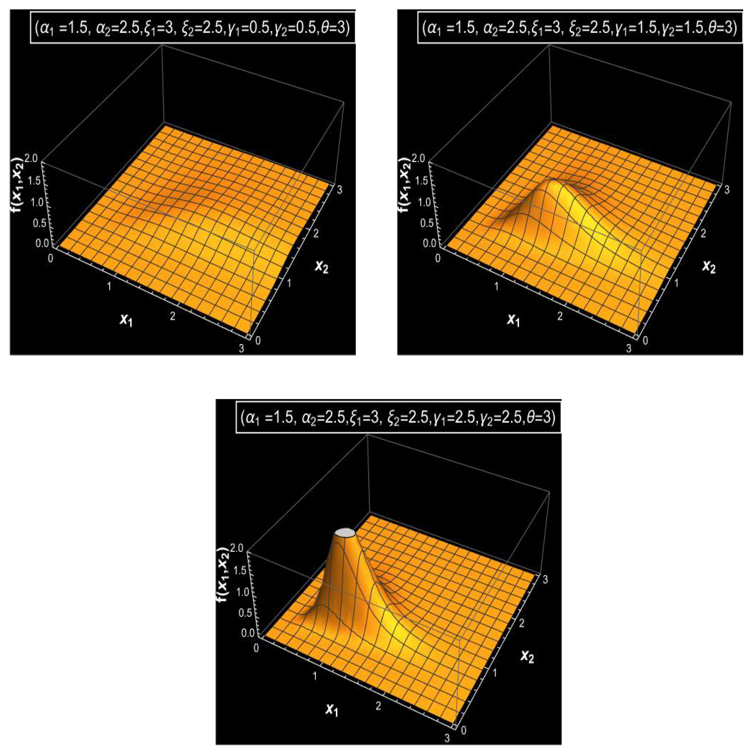
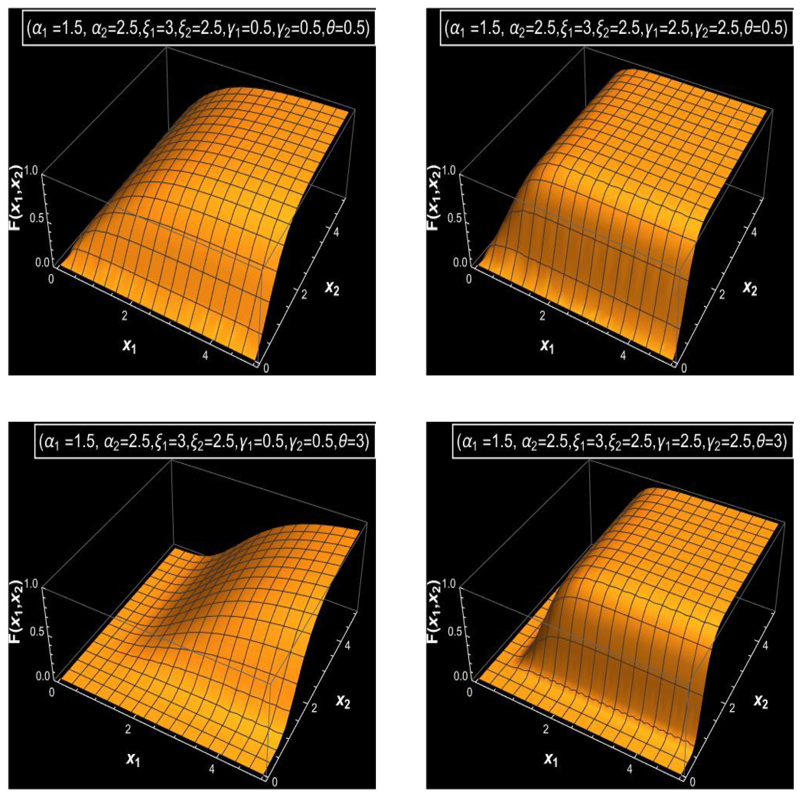
Figure 1, Figure 2 and Figure 3 display a graphical analysis of the bivariate MDD, illustrating its joint PDF and joint CDF under varying parameter settings to obtain a clear vision of the behavior of the bivariate MDD. These figures demonstrate how parameter changes affect the distribution’s shape and tail behavior. As the parameters increase, particularly ${\gamma }_1$ and ${\gamma }_2$, with fixed values of parameters ${\alpha }_1, {\alpha }_2, {\xi }_1$, and ${\xi }_2$ and a large value of $\theta$, Figure 1 illustrates that the distribution exhibits a sharper and narrower PDF peak. In contrast, with fixed values of parameters ${\alpha }_1, {\alpha }_2, {\xi }_1$ and ${\xi }_2$ and a large value of $\theta$, lower parameter values for ${\gamma }_1$ and ${\gamma }_2$ produce a flatter and wider PDF, as shown in Figure 1. Additionally, with a small value of $\theta$, one can show that the joint PDF of bivariate MDD has bi-modality or tri-modality shapes and also has a long right tail, as shown in Figure 2. The various shapes for the joint CDFs of bivariate MDD with various parameters $({\gamma }_1,{\gamma }_2,\theta )$ and fixed values of parameters ${\alpha }_1, {\alpha }_2, {\xi }_1$ and ${\xi }_2$ are shown in Figure 3. From Figure 3, we see that larger values of the parameter $\theta$ result in faster accumulation in the joint CDF for bivariate MDD, and smaller values of the parameter $\theta$ result in slower accumulation in the joint CDF for bivariate MDD.

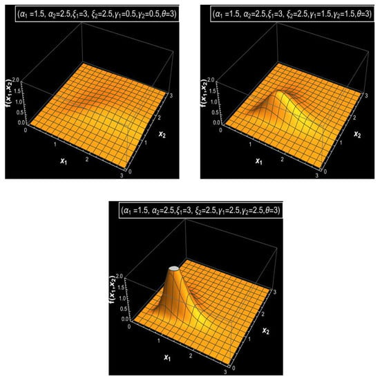
Figure 1. The joint PDFs of the bivariate MDD with different values of the parameters (${\gamma }_1=0.5$, $1.5, 2.5, {\gamma }_2=0.5, 1.5, 2.5, \theta =3$) and fixed value of parameters the ${\alpha }_1=1.5, {\alpha }_2=2.5, {\xi }_1=3$ and ${\xi }_2=2.5$.

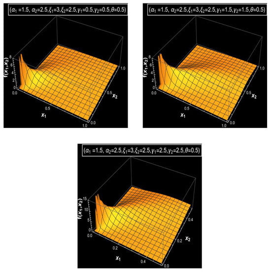
Figure 2. The joint PDFs of the bivariate MDD with different values of the parameters $({\gamma }_1=0.5,$$1.5, 2.5, {\gamma }_2=0.5, 1.5, 2.5, \theta =0.5)$ and fixed values of the parameters ${\alpha }_1=1.5, {\alpha }_2=2.5, {\xi }_1=3$, and ${\xi }_2=2.5$.

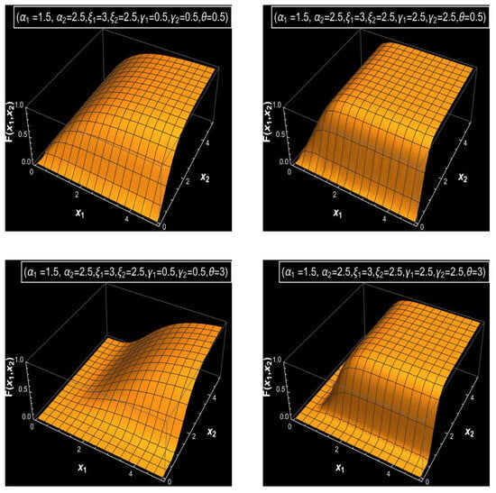
Figure 3. The joint CDFs of the bivariate MDD with different values of the parameters $({\gamma }_1=0.5, 2.5, {\gamma }_2=0.5, 2.5)$ and $\theta =0.5, 3$ and fixed values of the parameters ${\alpha }_1=1.5, {\alpha }_2=2.5, {\xi }_1=3$ and ${\xi }_2=2.5$.

3.4. Joint Survival Function

The traditional joint survival and the copula joint survival functions for MVMDD are derived in this subsection. These joint survival functions can be defined, respectively, as

$$\begin{array}{c}\hfill S(\mathit{x};\mathit{\alpha };\mathit{\xi };\mathit{\gamma };\theta )=P\left(\left(X_1\ge x_1\right)\cup \dots \cup \left(X_k\ge x_k\right)\right)=1-P\left(\left(X_1\le x_1\right)\cup \dots \cup \left(X_k\le x_k\right)\right),\end{array}$$

(20)

and

$$\begin{array}{c}\hfill S(\mathit{x};\mathit{\alpha };\mathit{\xi };\mathit{\gamma };\theta )={\overline{C}}_{\theta }(S\left(x_1\right),\dots ,S\left(x_k\right)).\end{array}$$

(21)

where $S\left(x_1\right)$, …, $S\left(x_k\right)$ are the marginal survival functions, which can be obtained from the marginal CDFs; for more details, see [26]. The following lemma presents the joint survival function for MVMDD and a formula for the joint survival functions based on the copula.

Lemma 4.

For $x_1>0$, …, $x_k>0$ and $S\left(x_1\right)$, …, $S\left(x_k\right)$ are the marginal survival functions; then, the joint survival function for MVMDD can be derived as

$$\begin{array}{ccc}\hfill S(\mathit{x};\mathit{\alpha };\mathit{\xi };\mathit{\gamma };\theta )& =& 1-\sum _{1\le i\le k}{\displaystyle \frac{1}{{(1+{\xi }_i{x}_i^{-{\alpha }_i}{e}^{-{\gamma }_i{x}_i})}^{\theta }}}\hfill \\ & +& \sum _{1\le i<j\le k}{\displaystyle \frac{1}{{(1+{\xi }_i{x}_i^{-{\alpha }_i}{e}^{-{\gamma }_i{x}_i}+{\xi }_j{x}_j^{-{\alpha }_j}{e}^{-{\gamma }_j{x}_j})}^{\theta }}}\hfill \\ & -& \dots +{(-1)}^{k+1}{\displaystyle \frac{1}{{(1+{\sum }_{i=1}^k{\phi }_i{x}_i^{-{\alpha }_i}{e}^{-{\gamma }_i{x}_i})}^{\theta }}}\hfill \\ & =& (1-k)+\sum _{1\le i\le k}S\left(x_i\right)+\sum _{1\le i<j\le k}{C}_{\theta }(1-S\left(x_i\right),1-S\left(x_j\right))\hfill \\ & -& \dots +{(-1)}^{k+1}{C}_{\theta }(1-S\left(x_1\right),\dots ,1-S\left(x_k\right)).\hfill \end{array}$$

(22)

Proof. 

Equation (22) can be obtained directly using the inclusion–exclusion identity [29]. □

4. Properties of the Proposed Distribution

In this section, some properties of MVMDD are discussed. The marginals of PDF and CDF for MVMDDs can be obtained in closed form and also classified as the PDF and CDF of MVMDDs. Additionally, the conditional distribution can be obtained for MVMDD, and the random samples can be generated from MVMDD.

Lemma 5.

For any MVMDD, the following properties are satisfied.

(i) 

Every marginal CDF obtained from MVMDD is also classified as the CDF of MVMDD.

(ii) 

Every marginal PDF obtained from MVMDD is also classified as PDF of MVMDD.

(iii) 

Every conditional distribution obtained from MVMDD is also classified as MVMDD and is given by

$$\begin{array}{ccc}\hfill f(x_1,\dots ,x_m|x_{m+1},\dots ,x_k)& =& {\displaystyle \frac{\Gamma (k+\theta )e^{-{\sum }_{i=1}^m{\gamma }_i{x}_i}{\prod }_{i=1}^m\left({\alpha }_i+{\gamma }_i{x}_i\right)x_i^{-{\alpha }_i-1}}{\Gamma (k+\theta -m)}}\hfill \\ & \times & \prod _{i=1}^m{\displaystyle \frac{{\xi }_i}{\left(1+{\sum }_{j=m+1}^k{\xi }_j{x}_j^{-{\alpha }_j}{e}^{-{\gamma }_j{x}_j}\right)}}\hfill \\ & \times & {\displaystyle \frac{1}{{\left(1+{\sum }_{i=1}^m\frac{{\xi }_i}{\left(1+{\sum }_{j=m+1}^k{\xi }_j{x}_j^{-{\alpha }_j}{e}^{-{\gamma }_j{x}_j}\right)}{x}_i^{-{\alpha }_i}{e}^{-{\gamma }_i{x}_i}\right)}^{k+\theta }}}\hfill \end{array}$$

which follows the MVMDD with joint PDF

$f(x_1,\dots ,x_m;{\alpha }_1,\dots ,{\alpha }_m;{\displaystyle \frac{{\xi }_1}{\left(1+{\sum }_{j=m+1}^k{\xi }_j{x}_j^{-{\alpha }_j}{e}^{-{\gamma }_j{x}_j}\right)}},\dots ,{\displaystyle \frac{{\xi }_m}{\left(1+{\sum }_{j=m+1}^k{\xi }_j{x}_j^{-{\alpha }_j}{e}^{-{\gamma }_j{x}_j}\right)}};{\gamma }_1,\dots ,{\gamma }_m;k+\theta -m)$.

Proof. 

To prove the preceding lemma, the following steps are required:

(i)

The proof for Lemma (5) (i) can be obtained directly from (19) as follows:

$$\begin{array}{ccc}\hfill F(\tilde{\mathit{x}};\tilde{\mathit{\alpha }};\tilde{\mathit{\xi }};\tilde{\mathit{\gamma }};\theta )& =& \underset{x_1\to \infty }{lim}{\displaystyle \frac{1}{{\left(1+{\sum }_{i=2}^k{\xi }_i{x}_i^{-{\alpha }_i}{e}^{-{\gamma }_i{x}_i}+{\xi }_1{x}_1^{-{\alpha }_1}{e}^{-{\gamma }_1{x}_1}\right)}^{\theta }}}\hfill \\ & =& {\displaystyle \frac{1}{{\left(1+{\sum }_{i=2}^k{\xi }_i{x}_i^{-{\alpha }_i}{e}^{-{\gamma }_i{x}_i}\right)}^{\theta }}},\hfill \end{array}$$

which is the joint CDF for MVMDD$(x_2,\dots ,x_k)$, and $\tilde{\mathit{x}}=(x_2,x_3,\dots ,x_n)$, $\tilde{\mathit{\alpha }}=({\alpha }_2,{\alpha }_3,\dots ,{\alpha }_n)$, $\tilde{\mathit{\xi }}=({\xi }_2,{\xi }_3,\dots ,{\xi }_n)$, and $\tilde{\mathit{\gamma }}=({\gamma }_2,{\gamma }_3,\dots ,{\gamma }_n)$.

(ii)

The proof for Lemma (5) (ii) can be obtained directly by integrating (17) from 0 to ∞ with respect to $x_i,i=1,2,3,\dots ,k$ as follows:

$$\begin{array}{ccc}\hfill f_{x_1}(\tilde{\mathit{x}};\tilde{\mathit{\alpha }};\tilde{\mathit{\xi }};\tilde{\mathit{\gamma }};\theta -1)& =& {\int }_0^{\infty }{\displaystyle \frac{\Gamma (k+\theta )}{\Gamma \left(\theta \right)}}{e}^{-{\sum }_{i=2}^k{\gamma }_i{x}_i}\prod _{i=2}^k{\xi }_i({\gamma }_i{x}_i+{\alpha }_i)x_i^{-{\alpha }_i-1}\hfill \\ & \times & {\displaystyle \frac{e^{-{\gamma }_1{x}_1}{\xi }_1({\gamma }_1{x}_1+{\alpha }_1)x_1^{-{\alpha }_1-1}}{{\left(1+{\sum }_{i=2}^k{\xi }_i{x}_i^{-{\alpha }_i}{e}^{-{\gamma }_i{x}_i}+{\xi }_1{x}_1^{-{\alpha }_1}{e}^{-{\gamma }_1{x}_1}\right)}^{k+\theta }}}d{x}_1,\hfill \\ & =& {\displaystyle \frac{\Gamma (k+\theta -1)}{\Gamma \left(\theta \right)}}{\displaystyle \frac{e^{-{\sum }_{i=2}^k{\gamma }_i{x}_i}{\prod }_{i=2}^k{\xi }_i({\gamma }_i{x}_i+{\alpha }_i)x_i^{-{\alpha }_i-1}}{{\left(1+{\sum }_{i=2}^k{\xi }_i{x}_i^{-{\alpha }_i}{e}^{-{\gamma }_i{x}_i}\right)}^{k+\theta -1}}},\hfill \end{array}$$

which is the joint PDF for MVMDD$(x_2,\dots ,x_k)$.

(iii)

The proof for Lemma (5) (iii) can be obtained directly from (17), and the proof of Lemma (5) (ii) is as follows:

$$\begin{array}{c}\hfill f(x_1,\dots ,x_m|x_{m+1},\dots ,x_k)={\displaystyle \frac{f(x_1,\dots ,x_k)}{f(x_{m+1},\dots ,x_k)}},\end{array}$$

where $f(x_1,\dots ,x_k)$ is given by (17) and $f(x_{m+1},\dots ,x_k)$ can be directly obtained from the proof of Lemma (5) (ii) as follows:

$$\begin{array}{c}\hfill f(x_{m+1},\dots ,x_k)={\displaystyle \frac{\Gamma (k+\theta -m)}{\Gamma \left(\theta \right)}}{\displaystyle \frac{e^{-{\sum }_{j=m+1}^k{\gamma }_j{x}_j}{\prod }_{j=m+1}^k{\xi }_j({\gamma }_j{x}_j+{\alpha }_j)x_j^{-{\alpha }_j-1}}{{\left(1+{\sum }_{j=m+1}^k{\xi }_j{x}_j^{-{\alpha }_j}{e}^{-{\gamma }_j{x}_j}\right)}^{k+\theta -m}}}.\end{array}$$

□

The following lemma can be used to generate random samples from MVMDD.

Lemma 6.

Let $f(x_1,\dots ,x_k)$ be the joint PDF of MVMDD, which is given by (17).

(i) 

The marginal PDF of $x_1$ and the conditional PDFs of $\left(x_2\right|x_1)$, $\left(x_3\right|x_2,x_1)$, …, $\left(x_k\right|x_1,\dots ,x_{k-1})$ are, respectively, given by

$$\begin{array}{ccc}\hfill f\left(x_1\right)& =& {\displaystyle \frac{\theta e^{-{\gamma }_1{x}_1}{\xi }_1({\gamma }_1{x}_1+{\alpha }_1)x_1^{-{\alpha }_1-1}}{{\left(1+{\xi }_1{x}_1^{-{\alpha }_1}{e}^{-{\gamma }_1{x}_1}\right)}^{\theta +1}}},\hfill \\ \hfill f\left(x_2\right|x_1)& =& {\displaystyle \frac{(\theta +1)e^{-{\gamma }_2{x}_2}{\xi }_2({\gamma }_2{x}_2+{\alpha }_2)x_2^{-{\alpha }_2-1}{\left(1+{\xi }_1{x}_1^{-{\alpha }_1}{e}^{-{\gamma }_1{x}_1}\right)}^{\theta +1}}{{\left(1+{\sum }_{i=1}^2{\xi }_i{x}_i^{-{\alpha }_i}{e}^{-{\gamma }_i{x}_i}\right)}^{\theta +2}}},\hfill \\ \hfill f\left(x_3\right|x_1,x_2)& =& {\displaystyle \frac{(\theta +2)e^{-{\gamma }_3{x}_3}{\xi }_3({\gamma }_3{x}_3+{\alpha }_3)x_3^{-{\alpha }_3-1}{\left(1+{\sum }_{i=1}^2{\xi }_i{x}_i^{-{\alpha }_i}{e}^{-{\gamma }_i{x}_i}\right)}^{\theta +2}}{{\left(1+{\sum }_{i=1}^3{\xi }_i{x}_i^{-{\alpha }_i}{e}^{-{\gamma }_i{x}_i}\right)}^{\theta +3}}},\hfill \\ & ⋮& \\ \hfill f\left(x_k\right|x_1,\dots ,x_{k-1})& =& {\displaystyle \frac{(\theta +k-1)e^{-{\gamma }_k{x}_k}{\xi }_k({\gamma }_k{x}_k+{\alpha }_k)x_k^{-{\alpha }_k-1}{\left(1+{\sum }_{i=1}^{k-1}{\xi }_i{x}_i^{-{\alpha }_i}{e}^{-{\gamma }_i{x}_i}\right)}^{\theta +k-1}}{{\left(1+{\sum }_{i=1}^k{\xi }_i{x}_i^{-{\alpha }_i}{e}^{-{\gamma }_i{x}_i}\right)}^{\theta +k}}}.\hfill \end{array}$$

(ii) 

The corresponding CDFs for the marginal PDF of $x_1$ and the conditional PDFs of $\left(x_2\right|x_1)$, $\left(x_3\right|x_2,x_1)$, …, $\left(x_k\right|x_1,\dots ,x_{k-1})$ are, respectively, given by

$$\begin{array}{ccc}\hfill F\left(x_1\right)& =& {\displaystyle \frac{1}{{\left(1+{\xi }_1{x}_1^{-{\alpha }_1}{e}^{-{\gamma }_1{x}_1}\right)}^{\theta }}},\hfill \\ \hfill F\left(x_2\right|x_1)& =& {\displaystyle \frac{{\left(1+{\xi }_1{x}_1^{-{\alpha }_1}{e}^{-{\gamma }_1{x}_1}\right)}^{\theta +1}}{{\left(1+{\sum }_{i=1}^2{\xi }_i{x}_i^{-{\alpha }_i}{e}^{-{\gamma }_i{x}_i}\right)}^{\theta +1}}},\hfill \\ \hfill F\left(x_3\right|x_1,x_2)& =& {\displaystyle \frac{{\left(1+{\sum }_{i=1}^2{\xi }_i{x}_i^{-{\alpha }_i}{e}^{-{\gamma }_i{x}_i}\right)}^{\theta +2}}{{\left(1+{\sum }_{i=1}^3{\xi }_i{x}_i^{-{\alpha }_i}{e}^{-{\gamma }_i{x}_i}\right)}^{\theta +2}}},\hfill \\ & ⋮& \\ \hfill F\left(x_k\right|x_1,\dots ,x_{k-1})& =& {\displaystyle \frac{{\left(1+{\sum }_{i=1}^{k-1}{\xi }_i{x}_i^{-{\alpha }_i}{e}^{-{\gamma }_i{x}_i}\right)}^{\theta +k-1}}{{\left(1+{\sum }_{i=1}^k{\xi }_i{x}_i^{-{\alpha }_i}{e}^{-{\gamma }_i{x}_i}\right)}^{\theta +k-1}}}.\hfill \end{array}$$

Proof. 

From Lemma 5 (ii and iii), Lemma 6 (i) can be easily proved. Additionally, Lemma 6 (ii) can be proved from Lemma 6 (i) by the traditional method. □

5. Multivariate Dependence Properties

In this section, we investigate the positively lower orthant dependent (PLOD) and lift rail decreasing (LTD) properties for MVMDD. First, we present some definitions for PLOD, and LTD is introduced; for more details, see [24,26].

Definition 1.

A multivariate random vector $(X_1,\dots ,X_k)$ is said to be PLOD iff $(X_1,\dots ,X_k)$ satisfies the following inequality:

$$\begin{array}{c}\hfill F(x_1,\dots ,x_k)\ge \prod _{i=1}^{k}F\left(x_i\right),\end{array}$$

where $F\left(x_i\right),i=1,\dots ,k$ are the marginal CDFs.

Definition 2.

Let $i=1,\dots ,m$ and $j=m+1,\dots ,k$. Then, $\left(X_j\right)$ is said to be LTD in $\left(X_i\right)$ if

$$\begin{array}{c}\hfill P(X_j\le x_j|X_i\le x_i),\end{array}$$

is a non-increasing function of $x_i$ for all $x_j$.

Lemma 7.

Let $f(x_1,\dots ,x_k)$ be the joint PDF of MVMDD given by (17); then, the random vector $(X_1,\dots ,X_k)$ is

(i) 

PLOD for MVMDD.

(ii) 

LTD for MVMDD.

Proof. 

To prove Lemma 7, the following steps are required:

(i)

To prove (i), we want to prove that

$$\begin{array}{c}\hfill {\left(1+\sum _{i=1}^k{\xi }_i{x}_i^{-{\alpha }_i}{e}^{-{\gamma }_i{x}_i}\right)}^{\theta }\prod _{i=1}^k{\displaystyle \frac{1}{{\left(1+{\xi }_i{x}_i^{-{\alpha }_i}{e}^{-{\gamma }_i{x}_i}\right)}^{\theta }}}\le 1,\end{array}$$

which can be written as

$$\begin{array}{c}\hfill \left(1+\sum _{i=1}^k{\xi }_i{x}_i^{-{\alpha }_i}{e}^{-{\gamma }_i{x}_i}\right)\prod _{i=1}^k{\displaystyle \frac{1}{\left(1+{\xi }_i{x}_i^{-{\alpha }_i}{e}^{-{\gamma }_i{x}_i}\right)}}\le 1,\end{array}$$

we use mathematical induction to prove this inequality. For $k=1$, the inequality is true. Consider the inequality is true when $k=l$. Now, we want to prove that the inequality is true if $k=l+1$. For $k=l+1$, the following inequality should be satisfied:

$$\begin{array}{c}\hfill \left(1+\sum _{i=1}^{l+1}{\xi }_i{x}_i^{-{\alpha }_i}{e}^{-{\gamma }_i{x}_i}\right)\prod _{i=1}^{l+1}{\displaystyle \frac{1}{\left(1+{\xi }_i{x}_i^{-{\alpha }_i}{e}^{-{\gamma }_i{x}_i}\right)}}\le 1.\end{array}$$

(23)

To prove the case of $k=l+1$, we can show from the case of $k=l$ that

$$\begin{array}{c}\hfill \left(1+\sum _{i=1}^l{\xi }_i{x}_i^{-{\alpha }_i}{e}^{-{\gamma }_i{x}_i}\right)\prod _{i=1}^{l+1}{\displaystyle \frac{1}{\left(1+{\xi }_i{x}_i^{-{\alpha }_i}{e}^{-{\gamma }_i{x}_i}\right)}}\le {\displaystyle \frac{1}{\left(1+{\xi }_{l+1}{x}_{l+1}^{-{\alpha }_{l+1}}{e}^{-{\gamma }_{l+1}{x}_{l+1}}\right)}},\end{array}$$

(24)

and

$$\begin{array}{c}\hfill \left({\xi }_{l+1}{x}_{l+1}^{-{\alpha }_{l+1}}{e}^{-{\gamma }_{l+1}{x}_{l+1}}\right)\prod _{i=1}^{l+1}{\displaystyle \frac{1}{\left(1+{\xi }_i{x}_i^{-{\alpha }_i}{e}^{-{\gamma }_i{x}_i}\right)}}\le 1-{\displaystyle \frac{1}{\left(1+{\xi }_{l+1}{x}_{l+1}^{-{\alpha }_{l+1}}{e}^{-{\gamma }_{l+1}{x}_{l+1}}\right)}}.\end{array}$$

(25)

From (24) and (25), one can show that (1) is satisfied.

(ii)

Using Definition 5.2 to prove (ii), let $i=1,\dots ,m$ and $j=m+1,\dots ,k$. Then,

$$\begin{array}{ccc}\hfill P(X_j\le x_j|X_i\le x_i)& =& {\displaystyle \frac{{\left(1+{\sum }_{i=1}^m{\xi }_i{x}_i^{-{\alpha }_i}{e}^{-{\gamma }_i{x}_i}\right)}^{\theta }}{{\left(1+{\sum }_{i=1}^k{\xi }_i{x}_i^{-{\alpha }_i}{e}^{-{\gamma }_i{x}_i}\right)}^{\theta }}}\hfill \\ & =& {\displaystyle \frac{1}{{\left(1+\frac{{\sum }_{i=m+1}^k{\xi }_i{x}_i^{-{\alpha }_i}{e}^{-{\gamma }_i{x}_i}}{1+{\sum }_{i=1}^m{\xi }_i{x}_i^{-{\alpha }_i}{e}^{-{\gamma }_i{x}_i}}\right)}^{\theta }}},\hfill \end{array}$$

(26)

which is a non-increasing function of $x_1,\dots ,x_m$ for all $x_{m+1},\dots ,x_k$.

□

6. Maximum Likelihood Estimation

Suppose that $x_{i1},\dots ,x_{ij}$ is an independent random sample of size s from $MVMDD(\Theta )$, where $\Theta =({\alpha }_1,\dots ,{\alpha }_k;{\xi }_1,\dots ,{\xi }_k;{\gamma }_1,\dots ,{\gamma }_k;\theta )$. From Equation (17), the likelihood function can be obtained as

$$\begin{array}{c}\hfill L(\Theta )={\left[{\displaystyle \frac{\Gamma (k+\theta )}{\Gamma \left(\theta \right)}}\prod _{i=1}^k{\xi }_i\right]}^n{\displaystyle \frac{{\prod }_{i=1}^k{\prod }_{j=1}^n{x}_{ij}^{-{\alpha }_i-1}({\alpha }_i+{\gamma }_i{x}_{ij})e^{-{\gamma }_i{x}_{ij}}}{{\prod }_{j=1}^n{\left(1+{\sum }_{i=1}^k{e}^{-{\gamma }_i{x}_{ij}}{\xi }_i{x}_{ij}^{-{\alpha }_i}\right)}^{k+\theta }}}.\end{array}$$

Then, the log likelihood function $\ell (\Theta )$ can be given as

$$\begin{array}{ccc}\hfill \ell (\Theta )& =& nlog\left[{\displaystyle \frac{\Gamma (k+\theta )}{\Gamma \left(\theta \right)}}\prod _{i=1}^k{\xi }_i\right]+log\prod _{i=1}^k\prod _{j=1}^n{x}_{ij}^{-{\alpha }_i-1}+log\prod _{i=1}^k\prod _{j=1}^n({\alpha }_i+{\gamma }_i{x}_{ij})\hfill \\ & +& log\prod _{i=1}^k\prod _{j=1}^n{e}^{-{\gamma }_i{x}_{ij}}-log\prod _{j=1}^n{\left(1+\sum _{i=1}^k{e}^{-{\gamma }_i{x}_{ij}}{\xi }_i{x}_{ij}^{-{\alpha }_i}\right)}^{k+\theta }.\hfill \end{array}$$

(27)

By taking the first derivative of (27) with respect to all parameters and equating the result to zero, the MLEs of the unknown parameters can be obtained by solving the (3k + 1) normal equations. The first derivatives of log-likelihood function can be derived for $i=1,2,\dots ,k$ as

$$\begin{array}{ccc}\hfill {\displaystyle \frac{\partial \ell }{\partial \theta }}& =& {\displaystyle \frac{n\Gamma \left(\theta \right)\left(\frac{\Gamma (k+\theta ){\psi }^{\left(0\right)}(k+\theta )}{\Gamma \left(\theta \right)}-\frac{{\psi }^{\left(0\right)}\left(\theta \right)\Gamma (k+\theta )}{\Gamma \left(\theta \right)}\right)}{\Gamma (k+\theta )}}-\sum _{j=1}^{n}log\left(\sum _{i=1}^k{\xi }_i{x}_{ij}^{-{\alpha }_i}{e}^{{\gamma }_i\left(-x_{ij}\right)}+1\right),\hfill \end{array}$$

(28)

$$\begin{array}{ccc}\hfill {\displaystyle \frac{\partial \ell }{\partial {\alpha }_i}}& =& \sum _{s=1}^k\sum _{j=1}^n{\displaystyle \frac{{\delta }_{i,s}}{{\gamma }_s{x}_{js}+{\alpha }_s}}+\sum _{s=1}^k\sum _{j=1}^n-{\delta }_{i,s}log\left(x_{js}\right)\hfill \\ & -& (\theta +k)\sum _{j=1}^n{\displaystyle \frac{{\sum }_{s=1}^k{\xi }_s{\delta }_{i,s}{x}_{js}^{-{\alpha }_s}\left(-e^{{\gamma }_s\left(-x_{js}\right)}\right)log\left(x_{js}\right)}{{\sum }_{i=1}^k{\xi }_i{x}_{ij}^{-{\alpha }_i}{e}^{{\gamma }_i\left(-x_{ij}\right)}+1}},\hfill \end{array}$$

(29)

$$\begin{array}{ccc}\hfill {\displaystyle \frac{\partial \ell }{\partial {\xi }_i}}& =& n\sum _{s=1}^k{\displaystyle \frac{{\delta }_{i,s}}{{\xi }_s}}-(\theta +k)\sum _{j=1}^n{\displaystyle \frac{{\sum }_{s=1}^k{\delta }_{i,s}{x}_{js}^{-{\alpha }_s}{e}^{{\gamma }_s\left(-x_{js}\right)}}{{\sum }_{i=1}^k{\xi }_i{x}_{ij}^{-{\alpha }_i}{e}^{{\gamma }_i\left(-x_{ij}\right)}+1}},\hfill \\ & \mathrm{a}\mathrm{n}\mathrm{d}& \end{array}$$

(30)

$$\begin{array}{ccc}\hfill {\displaystyle \frac{\partial \ell }{\partial {\gamma }_i}}& =& \sum _{s=1}^k\sum _{j=1}^n{\displaystyle \frac{x_{js}{\delta }_{i,s}}{{\gamma }_s{x}_{js}+{\alpha }_s}}-\sum _{s=1}^k\sum _{j=1}^n{x}_{js}{\delta }_{i,s}\hfill \\ & -& (\theta +k)\sum _{j=1}^n{\displaystyle \frac{{\sum }_{s=1}^k{\xi }_s{\delta }_{i,s}{x}_{js}^{1-{\alpha }_s}\left(-e^{{\gamma }_s\left(-x_{js}\right)}\right)}{{\sum }_{i=1}^k{\xi }_i{x}_{ij}^{-{\alpha }_i}{e}^{{\gamma }_i\left(-x_{ij}\right)}+1}},\hfill \end{array}$$

(31)

where ${\delta }_{i,s}=\left\{\begin{array}{cc}1\hfill & i=s,\hfill \\ 0\hfill & i\ne s,\hfill \end{array}\right.$ is the Kronecker delta function, ${\psi }^{\left(m\right)}\left(y\right)={\displaystyle \frac{d^{m+1}}{d{y}^{m+1}}}log\Gamma \left(y\right)$, and ($\Gamma \left(y\right)$ is the traditional gamma function), which are polygamma functions; see [30].

These (3k + 1) nonlinear equations in (28)–(31) cannot be solved analytically, so they can be solved numerically by the Newton–Raphson method using Mathematica 11; see Appendix B.

Fisher Information Matrix for MVMDD

Given the difficulty of computing the Fisher information matrix (which is obtained by taking the expectation of the second derivative of (27)), it would seem appropriate to use their MLEs to approximate these expected values. Then, as in [31], the asymptotic variance–covariance matrix is provided.

$$\begin{array}{c}\hfill \left(\begin{array}{cccccccc}Var\left(\widehat{\theta }\right)& Cov(\widehat{\theta },\widehat{{\alpha }_1})& Cov(\widehat{\theta },\widehat{{\alpha }_2})& \dots & Cov(\widehat{\theta },\widehat{{\xi }_1})& Cov(\widehat{\theta },\widehat{{\xi }_2})& \dots & Cov(\widehat{\theta },\widehat{{\gamma }_k})\\ Cov(\widehat{{\alpha }_1},\widehat{\theta })& Var\left(\widehat{{\alpha }_1}\right)& Cov(\widehat{{\alpha }_1},\widehat{{\alpha }_2})& \dots & & & & \\ Cov(\widehat{{\alpha }_2},\widehat{\theta })& Cov(\widehat{{\alpha }_2},\widehat{{\alpha }_3})& Var\left(\widehat{{\alpha }_2}\right)& \dots & & & & \\ .& & & & & & & \\ .& & & & & & & \\ .& & & & & & & \\ Cov(\widehat{{\gamma }_k},\widehat{\theta })& & & & & & & Var\left(\widehat{{\gamma }_k}\right)\end{array}\right)\\ \hfill ={\left(\begin{array}{cccccccc}-{\ell }_{\theta \theta }(\Theta )& -{\ell }_{\theta {\alpha }_1}(\Theta )& -{\ell }_{\theta {\alpha }_2}(\Theta )& \dots & -{\ell }_{\theta {\xi }_1}(\Theta )& -{\ell }_{\theta {\xi }_2}(\Theta )& \dots & -{\ell }_{\theta {\gamma }_k}(\Theta )\\ -{\ell }_{{\alpha }_1\theta }(\Theta )& -{\ell }_{{\alpha }_1{\alpha }_1}(\Theta )& -{\ell }_{{\alpha }_1{\alpha }_2}(\Theta )& \dots & & & & \\ -{\ell }_{{\alpha }_2\theta }(\Theta )& -{\ell }_{{\alpha }_2{\alpha }_1}(\Theta )& -{\ell }_{{\alpha }_2{\alpha }_2}(\Theta )& \dots & & & & \\ .& & & & & & & \\ .& & & & & & & \\ .& & & & & & & \\ {\ell }_{{\gamma }_k\theta }(\Theta )& & & & & & & {\ell }_{{\gamma }_k{\gamma }_k}(\Theta )\end{array}\right)}_{(\widehat{\theta }, \widehat{{\alpha }_l}, \widehat{{\xi }_l}, \widehat{{\gamma }_l})}^{-1},\end{array}$$

(32)

where ${\ell }_{{\theta }_i{\theta }_j}(\Theta )={\displaystyle \frac{{\partial }^2\ell }{\partial {\theta }_i{\theta }_j}},i,j=1,\dots ,(3k+1)$ are derived in Appendix A.

Consequently, for the parameters $\Theta$, the approximate CIs derived from the asymptotic variance–covariance matrix can be obtained from $(\widehat{{\theta }_l}\pm z_{{\displaystyle \frac{\alpha }{2}}}\sqrt{Var\left(\widehat{{\theta }_l}\right)}),l=1,\dots ,(3k+1)$, where the standard normal distribution’s percentile with right tail probability ${\displaystyle \frac{\alpha }{2}}$ is $z_{{\displaystyle \frac{\alpha }{2}}}$. The ACIs could produce a negative lower bound even when the parameters are positive. In this sense, zero might be used in place of the negative values.

7. Applications

In order to demonstrate the practical applications and effectiveness of the suggested model and the estimates, we provide an analysis of two real data sets, including protein consumption data [32] and warranty policy data [33]. For every data set, the MVMDD is compared with its sub-models MVDD, MVBIIID, and MVMBIIID and also with the following well-known multivariate distribution derived in [34].

The joint PDF of MVIWD proposed by [34], which is a multivariate distribution based on the class proposed by [23], is given as

$$\begin{array}{c}\hfill f(\mathit{x};\mathit{\alpha };\mathit{\xi };\theta )={\displaystyle \frac{\Gamma (k+\theta )}{\Gamma \left(\theta \right)}}{\displaystyle \frac{{\prod }_{i=1}^k\frac{{\xi }_i{\alpha }_i}{\theta }{x}_i^{-{\alpha }_i-1}{e}^{\frac{{\xi }_i}{\theta }{x}_i^{-{\alpha }_i}}}{{\left(1-k+{\sum }_{i=1}^k{e}^{\frac{{\xi }_i}{\theta }{x}_i^{-{\alpha }_i}}\right)}^{k+\theta }}},x_i>0,i=0,1,\dots ,k.\end{array}$$

The K-S test and the associated p-value are calculated for the marginals of the MVMDD, as well as of the marginals of its sub-models MVDD, MVBIIID, and MVMBIIID, and also of the marginals of MVIWD to determine how closely these distributions fit the data. This step is not sufficient to show that the MVMDD, MVDD, MVBIIID, and MVIWD fit the multivariate data or not, but it can be a guide for fitting (see [24]). Furthermore, the AIC is used to compare the candidate multivariate distributions.

7.1. Protein Consumption Data

Consider the data, which are the measurements in twenty-five European countries of protein consumption in nine food groups. The multivariate data were collected and are presented in [32], p. 535. In this paper, the data obtained from the measurements for four food groups (red meat, white meat, milk, and starch), summarized in Table 2, are analyzed to show the performance of the proposed multivariate distribution by comparing them with some sub-models, and MVIWD.

Table 2. Protein consumption in twenty-five European countries of data from four food groups.

Food Group	Measurements
Red meat	10.1, 8.9, 13.5, 7.8, 9.7, 10.6, 8.4, 9.5, 18.0, 10.2, 5.3, 13.9, 9.0, 9.5, 9.4, 6.9, 6.2, 6.2, 7.1,
	9.9, 13.1, 17.4, 9.3, 11.4, 4.4
White meat	1.4, 14., 9.3, 6., 11.4, 10.8, 11.6, 4.9, 9.9, 3.0, 12.4, 10.0, 5.1, 13.6, 4.7, 10.2, 3.7, 6.3,
	3.4, 7.8, 10.1, 5.7, 4.6, 12.5, 5.0
Milk	8.9, 19.9, 17.5, 8.3, 12.5, 25.0, 11.1, 33.7, 19.5, 17.6, 9.7, 25.8, 13.7, 23.4, 23.3, 19.3, 4.9,
	11.1, 8.6, 24.7, 23.8, 20.6, 16.6, 18.8, 9.5
Starch	0.6, 3.6, 5.7, 1.1, 5.0, 4.8, 6.5, 5.1, 4.8, 2.2, 4.0, 6.2, 2.1, 4.2, 4.6, 5.9, 5.9, 3.1,
	5.7, 3.7, 2.8, 4.7, 6.4, 5.2, 3.0

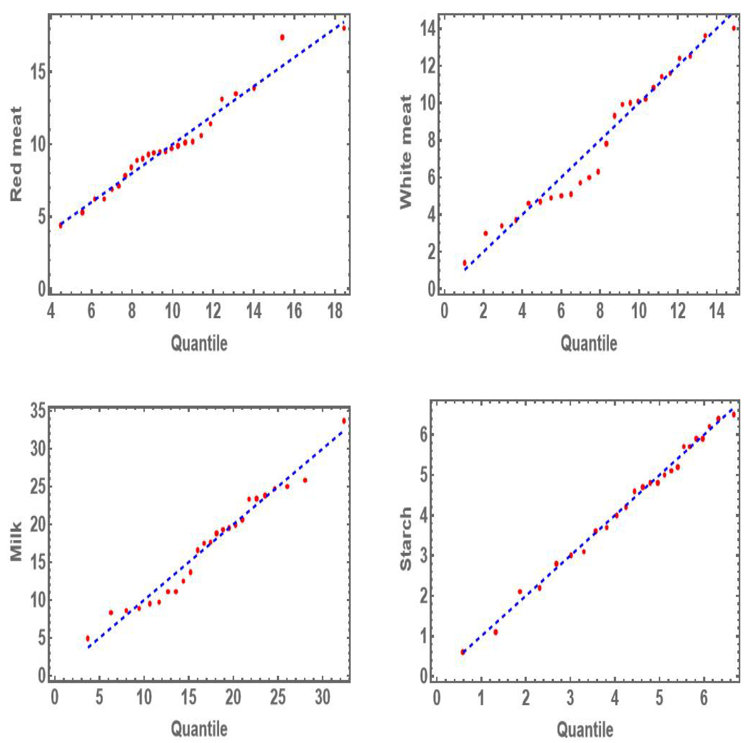
Table 3 shows the values of K-S distance with the associated p-value for the marginal distributions and IWD. From Table 3, one can show that the marginal distributions for MDD, DD, BIIID, and IWD fit all univariate data sets well based on the values of p-value. So we can say that the MVMDD, MVDD, MVBIIID, and MVIWD are suitable models for the multivariate data. The Q-Q plots are used to validate marginal distributions for all data sets of the protein consumption data before estimating the multivariate distribution. Figure 4 shows the Q-Q plots for four data sets of the protein consumption data. From Figure 4, it is evident that the marginal distribution of MVMDD fits all four data sets of the protein consumption data well.

Table 3. K-S test distance with the associated p-value for the protein consumption data.

Uni-Variate Model	Data	K-S	p-Value
	Red meat	0.1087	0.9289
MDD	White meat	0.1566	0.5719
	Milk	0.1228	0.8450
	Starch	0.0775	0.9982
	Red meat	0.1057	0.9427
DD	White meat	0.1551	0.5841
	Milk	0.1222	0.8496
	Starch	0.0594	0.9999
	Red meat	0.1397	0.7133
BIIID	White meat	0.1863	0.3507
	Milk	0.1584	0.5571
	Starch	0.2528	0.0819
	Red meat	0.1402	0.7094
IWD	White meat	0.1926	0.3118
	Milk	0.1579	0.5607
	Starch	0.2748	0.0458

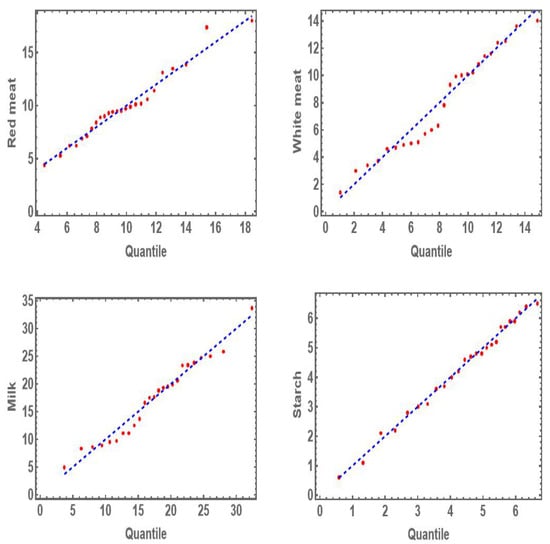
Figure 4. Q-Q plot the four food groups in the protein consumption data.

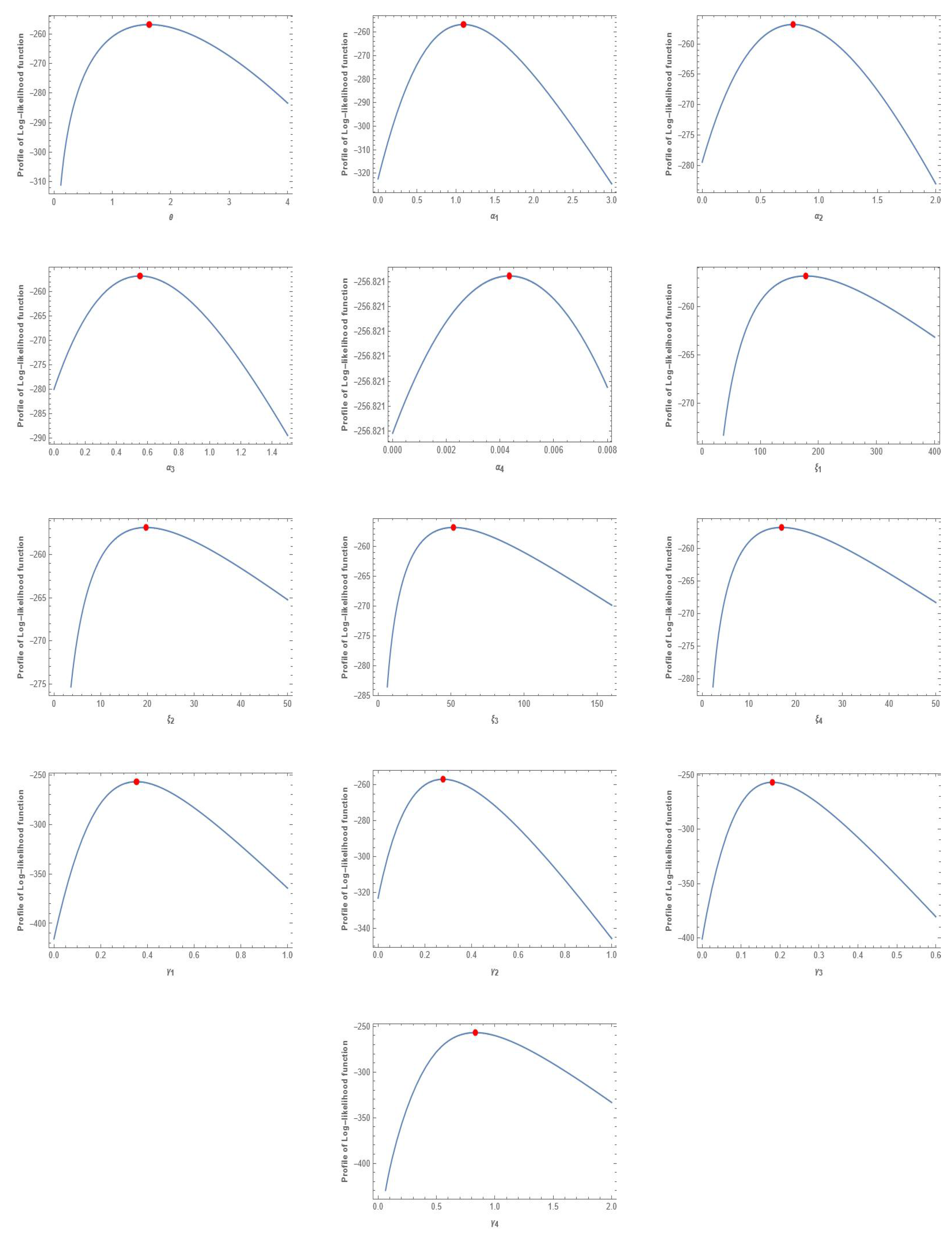
The MLEs for the unknown parameters of MVMDD, MVDD, MBIIID, and MVIWD are obtained when the multivariate protein consumption data are used. Table 4 displays the values of the MLEs for MVMDD, MVDD, MBIIID, and MVIWD, and the associated values for AIC. Based on the values of the AICs for MVMDD, MVDD MVBIIID, and MVIWD, it is evident that MVMDD has the lowest value and is considered better than the other models. Additionally, the plots of the profile log-likelihood function of the estimated parameters for the protein consumption data are shown in Figure 5.

Table 4. The estimates of the unknown parameters of MVMDD, MVDD, MBIIID, and MVIWD with the associated values of AIC for the protein consumption data.

Parameters	MVMDD	MVDD	MVBIIID	MVIWD
$\widehat{\theta }$	1.6308	1.1288	12.739	4.1003
${\widehat{\alpha }}_1$	1.0964	4.2861	1.3394	2.9045
${\widehat{\alpha }}_2$	0.7791	2.7456	1.5348	1.6371
${\widehat{\alpha }}_3$	0.5523	3.2721	1.0836	1.9949
${\widehat{\alpha }}_4$	0.0043	2.5119	1.9857	1.4102
${\widehat{\xi }}_1$	178.32	11,304.7	1	388.45
${\widehat{\xi }}_2$	19.689	167.517	1	15.147
${\widehat{\xi }}_3$	51.726	7260.55	1	153.48
${\widehat{\xi }}_4$	17.008	24.6011	1	4.2682
${\widehat{\gamma }}_1$	0.3534	0	0	-
${\widehat{\gamma }}_2$	0.2782	0	0	-
${\widehat{\gamma }}_3$	0.1804	0	0	-
${\widehat{\gamma }}_4$	0.8316	0	0	-
AIC	539.64	554.88	633.29	585.77

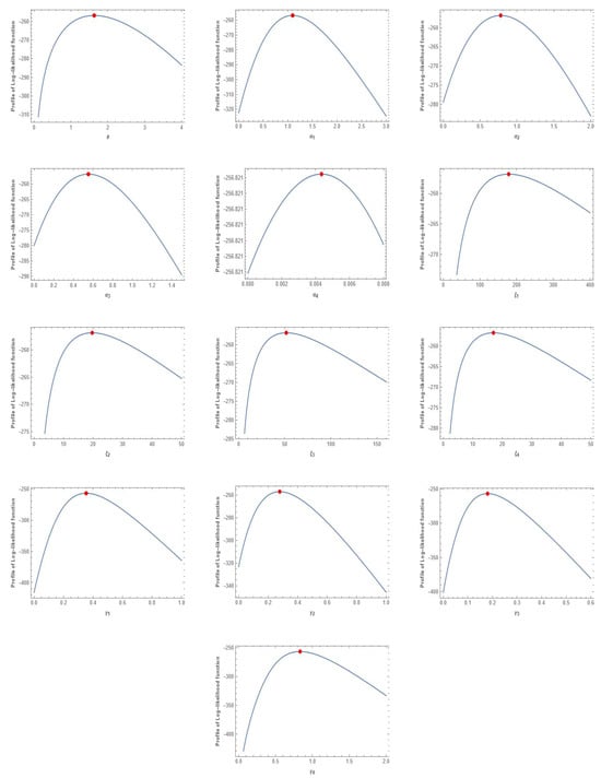
Figure 5. The log-likelihood function of the estimated parameters of MVMDD for the protein consumption data.

The calculated variance–covariance matrix of the unknown parameters based on the protein consumption data is presented in Appendix A. The 95% and 90% ACIs using the calculated variance–covariance matrix are computed for the unknown parameters of MVMDD for the protein consumption data and reported in Table 5.

Table 5. The 95% and 90% ACIs of the unknown parameters of MVMDD for the protein consumption data.

Parameters	$95\%\mathit{ACI}$	$90\%\mathit{ACI}$
$\theta$	(0.3269, 2.9347)	(0.5365, 2.7251)
${\alpha }_1$	(0.0, 5.4175)	(0.0, 4.7231)
${\alpha }_2$	(0.0, 2.2795)	(0.0, 2.0383)
${\alpha }_3$	(0.0, 2.7776)	(0.0, 2.4200)
${\alpha }_4$	(0.0, 0.9644)	(0.0, 0.8101)
${\xi }_1$	(0.0, 1131.7)	(0.0, 978.45)
${\xi }_2$	(0.0, 58.645)	(0.0, 52.385)
${\xi }_3$	(0.0, 258.65)	(0.0, 225.39)
${\xi }_4$	(0.0, 43.912)	(0.0, 43.912)
${\gamma }_1$	(0.0, 0.8653)	(0.0, 0.7831)
${\gamma }_2$	(0.0249, 0.5314)	(0.0656, 0.4907)
${\gamma }_3$	(0.013, 0.3478)	(0.0399, 0.3209)
${\gamma }_4$	(0.4226, 1.2407)	(0.4883, 1.1750)

7.2. Data for Warranty Policies 

Consider the bivariate real data set from [33] consisting of 30 observations of failure times and warranty servicing times in days for nuclear power plants of the four nuclear sites in South Korea. Recently, [35] analyzed this data using the bivariate exponentiated additive Weibull distribution. In this subsection, the bivariate real data, summarized in Table 6, are analyzed to show the performance of the proposed bivariate distribution by comparing them with some sub-models and the bivariate IWD.

Table 6. Failure times and warranty servicing times for nuclear power plants.

	Measurements
Failure times	353.04, 334.72, 80.04, 6.49, 1.34, 467.19, 0.35, 398.86, 1048.23, 829.23,
	227.20, 260.14, 14.00, 14.15, 38.96, 30.27, 117.37, 126.27, 56.45, 45.28,
	267.31, 615.64, 115.37, 359.76, 412.30, 276.69, 601.04, 1021.01, 192.17, 0.36
Warranty servicing	4.37, 1.91, 2.04, 1.72, 0.29, 1.93, 1.82, 1.77, 9.61, 3.80, 2.86, 0.31, 0.85,
times	2.04, 2.73, 3.63, 2.73, 2.55, 0.72, 3.69, 0.36, 10.63, 11.24, 9.70, 3.31, 4.96,
	2.99, 2.36, 1.63, 0.26

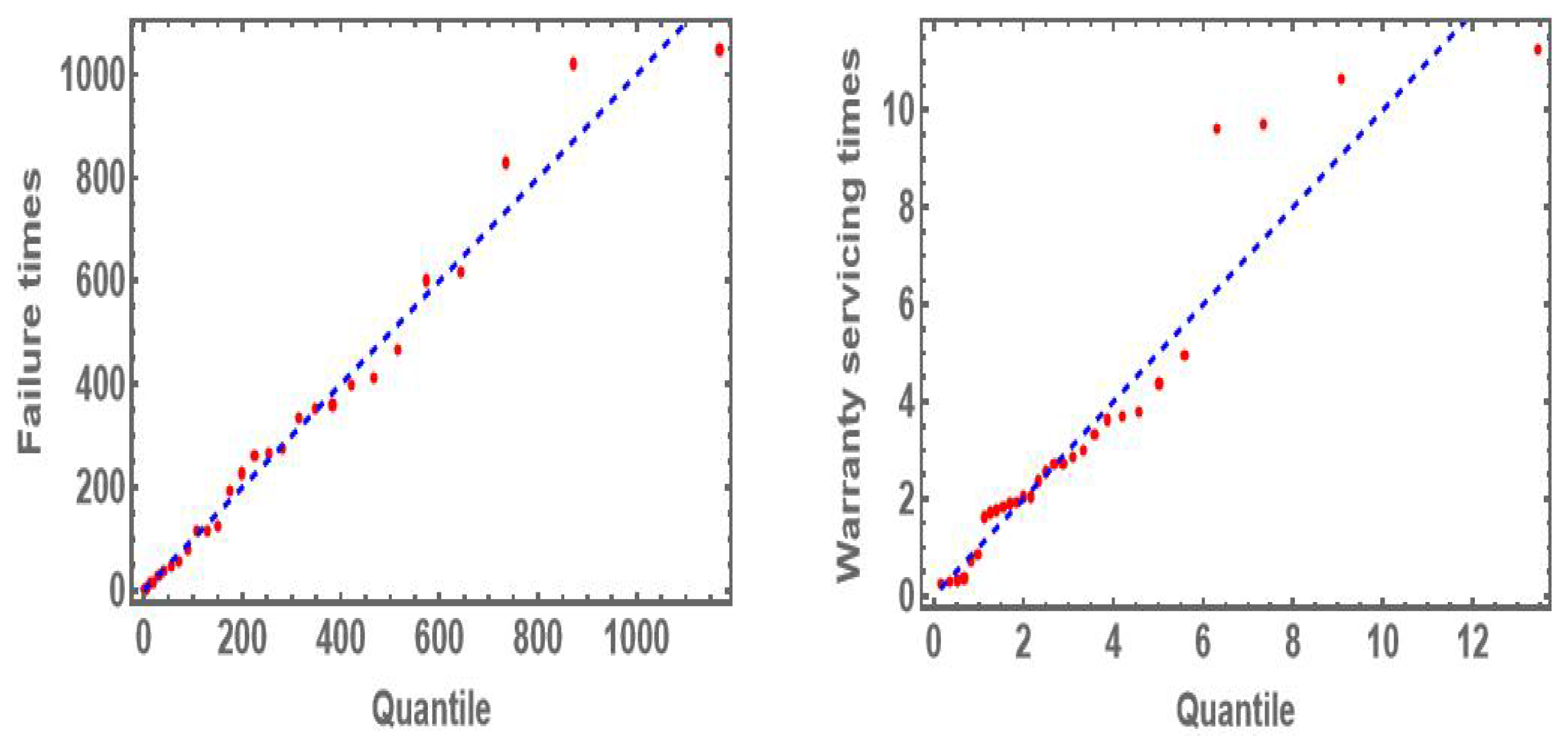
The numerical values of the K-S test and the associated p-value of all comparison uni-variate distributions (marginal functions) are summarized in Table 7 for warranty policy data. It is evident from Table 7 that the marginal distributions for all comparison distributions fit all univariate data sets well based on the p-values. Figure 6 shows the Q-Q plots for two data sets of the warranty policies data. From Figure 6, it is evident that the marginal distribution of MVMDD fits both data sets of the warranty policies data well.

Table 7. K-S test distance with the associated p-value for the warranty policy data.

Uni-Variate Model	Data	K-S	p-Value
MDD	Failure times	0.0580	0.9999
	Warranty servicing	0.1029	0.9087
DD	Failure times	0.0671	0.9993
	Warranty servicing	0.1004	0.9231
BIIID	Failure times	0.2019	0.1733
	Warranty servicing	0.1785	0.2947
MBIIID	Failure times	0.0471	0.9999
	Warranty servicing	0.1149	0.8231
IWD	Failure times	0.2189	0.1127
	Warranty servicing	0.2178	0.1162

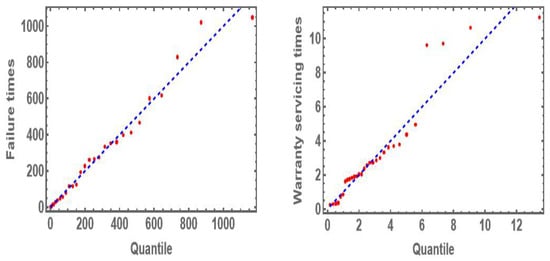
Figure 6. Q-Q plot for failure times and warranty servicing times in days of the warranty policy data.

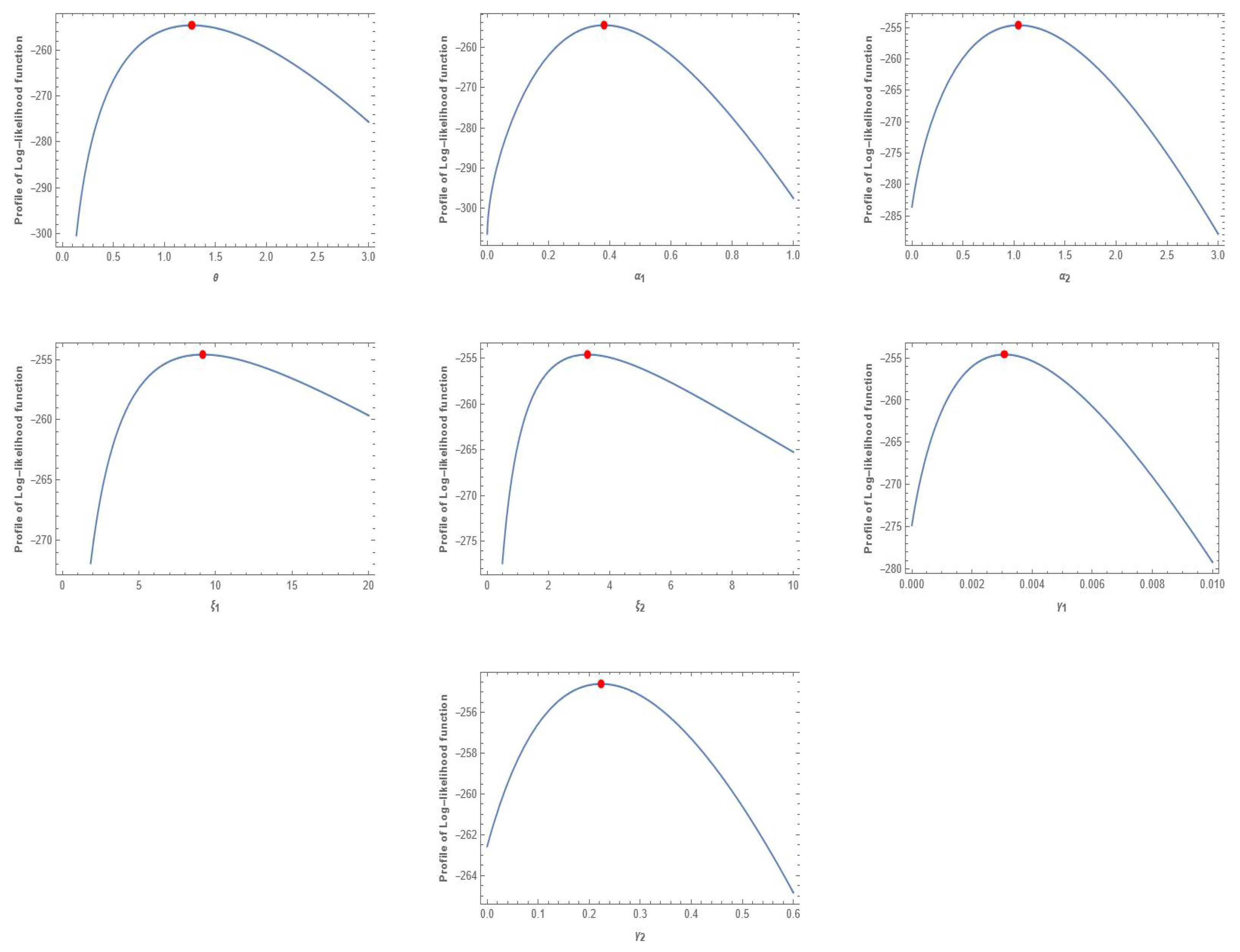
The MLEs for the unknown parameters of MVMDD, MVDD, MVBIIID, MVMBIIID, and MVIWD are obtained when the multivariate warranty policies data are used. Table 8 shows the values of the MLEs for MVMDD, MVDD, MVBIIID, MVMBIIID, and MVIWD, and the associated values for AIC. Based on the values of the AICs for MVMDD, MVDD MVBIIID, MVMBIIID, and MVIWD, it is evident that MVMDD and MVMBIIID have the lowest values and are considered better than other models for the warranty policy data. Additionally, the plots of the profile log-likelihood function of the estimated parameters for the protein consumption data are shown in Figure 7.

Table 8. The estimates of the unknown parameters of MVMDD, MVDD, MVBIIID, MVMBIIID, and MVIWD with the associated AICs for the warranty policy data.

Parameters	MVMDD	MVDD	MVBIIID	MVMBIIID	MVIWD
$\widehat{\theta }$	1.2674	0.6852	2.8541	0.2018	2.0508
${\widehat{\alpha }}_1$	0.3823	0.8720	0.3801	6.7665	0.3905
${\widehat{\alpha }}_2$	1.0443	1.9513	1.3011	0.5389	0.9647
${\widehat{\xi }}_1$	9.1664	103.04	1	1	3.6936
${\widehat{\xi }}_2$	3.2762	8.8347	1	1	1.2767
${\widehat{\gamma }}_1$	0.0031	0	0	0.0032	-
${\widehat{\gamma }}_2$	0.2234	0	0	0.3712	-
AIC	523.20	535.74	566.84	523.88	558.47

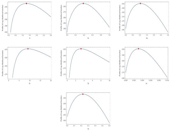
Figure 7. The log-likelihood function of estimated parameters of MVMDD for the warranty policy data.

The 95% and 90% ACIs using the asymptotic variance–covariance matrix, given in Box 2, are computed for the unknown parameters of MVMDD for warranty policy data and are reported in Table 9.

Table 9. The 95% and 90% ACIs for the unknown parameters of MVMDD for the warranty policy data.

Parameters	$95\%\mathit{ACI}$	$90\%\mathit{ACI}$
$\theta$	(0.0, 2.6387)	(0.1165, 2.4183)
${\alpha }_1$	(0.1129, 0.6518)	(0.1562, 0.6085)
${\alpha }_2$	(0.2292, 1.8594)	(0.3602, 1.7284)
${\xi }_1$	(0.0, 31.082)	(0.0, 27.5596)
${\xi }_2$	(0.0, 9.1585)	(0.0, 8.2131)
${\gamma }_1$	(0.0012, 0.0049)	(0.0015, 0.0046)
${\gamma }_2$	(0.0249, 0.4942)	(0.0656, 0.4507)

8. Conclusions

In this paper, we introduced MVMDD and its sub-models with MDD, DD, MBIIID, and BIIID as their respective marginals. The proposed model is highly flexible, allowing it to be derived in two distinct ways for both the PDF and the CDF. We explored various properties of the model in detail, providing a thorough understanding of its characteristics. While the MLEs are computationally intensive, we employed a numerical method to facilitate their estimation. To illustrate the applicability of the model, we analyzed multivariate protein consumption in a data set of twenty-five European countries and warranty policy data, consisting of 30 observations of failure times and warranty servicing times in days for nuclear power plants of the four nuclear sites in South Korea. The results demonstrated that the proposed model fits the two data sets well, outperforming its sub-models and MVIWD in terms of the AIC value. This indicates that the proposed model provided a better fit for these particular data sets. Overall, the paper showcases the flexibility and practical utility of the model for real-world data analysis. The proposed model offered a promising approach for modeling multivariate data with specific marginal distributions.

References

- Keller, A.Z.; Kamath, A.R.R.; Perera, U.D. Reliability analysis of cnc machine tools. Reliab. Eng. 1982, 3, 449–473. [Google Scholar] [CrossRef]
- Calabria, R.; Pulcini, G. Bayes 2-sample prediction for the inverse Weibull distribution. Commun. Stat.-Theory Methods 1994, 23, 1811–1824. [Google Scholar] [CrossRef]
- Johnson, N.L.; Kotz, S.; Balakrishnan, N. Continuous Univariate Distributions, Volume 1; Wiley Series in Probability and Statistics; Wiley: Hoboken, NJ, USA, 1994. [Google Scholar]
- Jana, N.; Bera, S. Estimation of parameters of inverse Weibull distribution and application to multi-component stress-strength model. J. Appl. Stat. 2022, 49, 169–194. [Google Scholar] [CrossRef] [PubMed]
- de Gusmão, F.R.S.; Ortega, E.M.M.; Cordeiro, G.M. The generalized inverse Weibull distribution. Stat. Pap. 2011, 52, 591–619. [Google Scholar] [CrossRef]
- Lai, C.D.; Xie, M.; Murthy, D.N.P. A modified Weibull distribution. IEEE Trans. Reliab. 2003, 52, 33–37. [Google Scholar] [CrossRef]
- Peng, X.; Yan, Z. Estimation and application for a new extended Weibull distribution. Reliab. Eng. Syst. Saf. 2014, 121, 34–42. [Google Scholar] [CrossRef]
- Dagum, C. A new model of personal income distribution: Specification and estimation. Écon. Appl. 1977, 30, 413–437. [Google Scholar] [CrossRef]
- Kleiber, C. A Guide to the Dagum Distributions; Springer: New York, NY, USA, 2008; pp. 97–117. [Google Scholar]
- Oluyede, B.; Huang, S.; Pararai, M. A new class of generalized Dagum distribution with applications to income and lifetime data. J. Stat. Econom. Methods 2014, 3, 121–151. [Google Scholar]
- Mansoor, M.; Zubair, M.; Tahir, M.H.; Cordeiro, G.M.; Alizadeh, M. The Weibull-Dagum distribution: Properties and applications. Commun. Stat.-Theory Methods 2016, 45, 7376–7398. [Google Scholar]
- Domma, F.; Condino, F.; Giordano, S. A new formulation of the Dagum distribution in terms of income inequality and poverty measures. Phys. A Stat. Mech. Its Appl. 2018, 511, 104–126. [Google Scholar] [CrossRef]
- Nasiru, S.; Mwita, P.N.; Ngesa, O. Exponentiated generalized exponential Dagum distribution. J. King Saud Univ.-Sci. 2019, 31, 362–371. [Google Scholar] [CrossRef]
- Bhatti, F.A.; Hamedani, G.G.; Korkmaz, M.C.; Ahmad, M. On the new modified Dagum distribution: Properties and applications. J. Stat. Manag. Syst. 2020, 23, 1513–1542. [Google Scholar] [CrossRef]
- Jamal, F.; Abuzaid, A.H.; Tahir, M.H.; Nasir, M.A.; Khan, S.; Mashwani, W.K. New modified Burr-III distribution, properties and applications. Math. Comput. Appl. 2021, 26, 82. [Google Scholar] [CrossRef]
- Tablada, C.J.; Cordeiro, G.M. The modified Fréchet distribution and its properties. Commun. Stat.-Theory Methods 2017, 46, 10617–10639. [Google Scholar] [CrossRef]
- Burr, I.W. Cumulative Frequency Functions. Ann. Math. Stat. 1942, 13, 215–232. [Google Scholar] [CrossRef]
- Mokhlis, N.A. Reliability of a stress-strength model with Burr Type-III distributions. Commun. Stat.-Theory Methods 2005, 34, 1643–1657. [Google Scholar] [CrossRef]
- Gove, J.H.; Ducey, M.J.; Leak, W.B.; Zhang, L. Rotated sigmoid structures in managed uneven-aged northern hardwood stands: A look at the Burr-Type-III distribution. For. Int. J. For. Res. 2008, 81, 161–176. [Google Scholar] [CrossRef]
- Hassan, A.S.; Elsherpieny, E.A.; Aghel, W.E. Statistical inference of the Burr Type-III distribution under joint progressively Type-II censoring. Sci. Afr. 2023, 21, e01770. [Google Scholar] [CrossRef]
- Mardia, K.V. Multivariate Pareto distributions. Ann. Math. Stat. 1962, 33, 1008–1015. [Google Scholar] [CrossRef]
- Takahasi, K. Note on the multivariate Burr’s distribution. Ann. Inst. Stat. Math. 1965, 17, 257–260. [Google Scholar] [CrossRef]
- El-Hussaini, E.K.; Ateya, S.F. A class of multivariate distributions and new copulas. J. Egypt. Math. Soc. 2006, 14, 45–54. [Google Scholar]
- Kundu, D.; Kumar, A.; Gupta, A.K. Absolute continuous multivariate generalized exponential distribution. Sankhya Indian J. Stat. Ser. B 2015, 77, 175–206. [Google Scholar] [CrossRef]
- Sarabia, J.M.; Jorda, V.; Prieto, F.; Guillen, M. Multivariate classes of GB2 distributions with applications. Mathematics 2021, 9, 72. [Google Scholar] [CrossRef]
- Nelsen, R.B. An Introduction to Copulas; Springer Series in Statistics; Springer: New York, NY, USA, 2007. [Google Scholar]
- Yari, G.; Djafari, A.M. Information covariance matrices for multivariate Burr III and logistic distributions. Int. J. Ind. Eng. Prod. Res. 2008, 19, 2–5+9–20. [Google Scholar]
- Malik, H.J.; Abraham, B. Multivariate Logistic Distributions. Ann. Stat. 1973, 1, 588–590. [Google Scholar] [CrossRef]
- Sane, S.S. The Inclusion-Exclusion Principle; Hindustan Book Agency: Gurgaon, India, 2013; pp. 57–79. [Google Scholar]
- Gradshteyn, I.S.; Ryzhik, I.M. Table of Integrals, Series, and Products, 7th ed.; Translated from the Russian, Translation Edited and with a Preface by Alan Jeffrey and Daniel Zwillinger, with One CD-ROM (Windows, Macintosh and UNIX); Elsevier/Academic Press: Amsterdam, The Netherlands, 2007. [Google Scholar]
- Cohen, A.C. Maximum likelihood estimation in the Weibull distribution based on complete and on censored samples. Technometrics 1965, 7, 579–588. [Google Scholar] [CrossRef]
- Timm, N.H. Applied Multivariate Analysis; Springer Texts in Statistics; Springer: New York, NY, USA, 2002. [Google Scholar]
- Park, M.; Kim, J.-Y. Cost analysis on warranty policies using freund’s bivariate exponential distribution. J. Korean Soc. Qual. Manag. 2014, 42, 1–14. [Google Scholar] [CrossRef]
- Hassan, M.; Aslam, M. Dus- neutrosophic multivariate inverse weibull distribution: Properties and applications. Complex Intell. Syst. 2023, 9, 5679–5691. [Google Scholar] [CrossRef]
- Poonia, N.; Prajapati, D.; Azad, S. The bivariate exponentiated additive weibull distribution and its multivariate extension with applications. Comput. Ind. Eng. 2024, 188, 109886. [Google Scholar] [CrossRef]
Disclaimer/Publisher’s Note: The statements, opinions and data contained in all publications are solely those of the individual author(s) and contributor(s) and not of MDPI and/or the editor(s). MDPI and/or the editor(s) disclaim responsibility for any injury to people or property resulting from any ideas, methods, instructions or products referred to in the content. |
© 2025 by the authors. Licensee MDPI, Basel, Switzerland. This article is an open access article distributed under the terms and conditions of the Creative Commons Attribution (CC BY) license (https://creativecommons.org/licenses/by/4.0/).