Abstract
This study investigated the sensitivity of maximum torque per ampere (MTPA) control in synchronous reluctance machines (SynRMs) to angle errors, examining specifically how deviations in the reference control trajectory affected performance. Analytical and numerical methods were employed to analyze this sensitivity systematically, including the impact of magnetic saturation. Two MTPA control implementation schemes were evaluated, with torque and current amplitude as the reference variables, using a template SynRM from the open-source simulation tool SyR-e. The results indicated that performance sensitivity to angle errors was moderately low near the MTPA trajectory, allowing for significant angle deviations with minimal performance loss. Although magnetic saturation increased this sensitivity slightly, reducing the allowable error range by up to 25%, the maximum angle deviation for up to 1% of the performance decrease still corresponded to approximately around the MTPA trajectory. The findings of this study suggest potential for simplifying control implementations, reducing component costs through less precise position determination (sensor-based or sensorless), and achieving additional control objectives such as torque ripple reduction.
Keywords:
control angle error; finite element method; MTPA control; sensitivity to performance decrease; suboptimal operation; synchronous reluctance machines MSC:
93-08
1. Introduction
Since the 1980s, permanent magnet (PM) synchronous machines have been the focus of extensive research for high-performance drive applications. However, especially in the last decade, synchronous reluctance machines (SynRMs) have also attracted significant interest due to their unique advantages and the challenges of the permanent magnet industry [1,2,3,4,5]. The scientific and industrial sectors’ increasing interest in SynRMs is driven primarily by the shift toward technologies that do not depend on rare-earth elements and a demand for more energy-efficient electric machines [1,5,6]. In this respect, SynRMs have great potential, because they do not require magnets or field excitation. They are promising for applications requiring high efficiency, dynamic performance, and low cost due to their rotor structure, which consists of a stack of laminations without excitation coils, short-circuited conductors, or PMs [1,5,6]. SynRMs offer further advantages, including a wide constant power speed range, position detection at zero speed by exploiting rotor magnetic saliency, and no risk of demagnetization [1,2,3,5,7,8]. Due to these advantages, SynRMs are excellent candidates for widespread use across various industries, including for fans and pumps, compressors, elevators, centrifugal machines, conveyor systems, and cranes, among others [2].
The potential of SynRMs has already been recognized in the industrial sector, as leading manufacturers such as Siemens, ABB, and KSB already offer serial high-efficiency SynRMs for industrial use. In addition, there is considerable potential for their use in automotive applications [1]. However, the deployment of SynRMs in high-performance drives, such as electric vehicles, is challenged by high torque ripple, causing increased acoustic noise and vibration [6,9]. Further drawbacks of SynRMs are, e.g., lower efficiency, torque/power density, power factor, and constant power speed range in comparison to well-designed PM synchronous machines [1,2,3,5,7,8].
There are several open challenges regarding SynRMs. Finite element method (FEM) analysis is generally used for the design and optimization of the discussed machines [3,4,5,7,9,10,11,12,13,14]. The main challenges include multiphysics designing and optimizing the complex anisotropic structure of the rotor, improving the power factor, and minimizing torque ripple, rotor iron losses, vibration, and noise [1,6,12,14,15]. Research on SynRM motor control methods has also experienced significant growth, aiming to achieve higher performance and efficiency of SynRM drives. The dominant approach is applying the so-called vector control methods, where the research is directed towards decreasing position estimation error, minimizing torque ripple, achieving high accuracy and dynamic performance, and increasing motor efficiency [2,8,9,16,17,18,19,20,21,22,23,24,25,26]. In general, sensor faults remain a common problem that decreases the reliability of electrical drives. Therefore, various sensorless control methods are researched and applied [2,8,17,18,22]. Regarding control strategies, the main focus at speeds up to nominal speeds is optimizing conduction power losses (i.e., Joule losses), which are the most significant in this operating range. Such a strategy is known as the maximum torque per ampere (MTPA) control strategy [2,15,19,20,24,25,27,28,29,30,31,32,33]. This strategy provides the minimum current for a given torque, although the total power loss may not be minimized. Regardless, this strategy is generally considered optimal due to its simplicity because additional consideration of iron losses is challenging [19,20]. MTPA methods can be divided into online and offline techniques and various implementations [2,15,19,20,24,25,27,28,29,30,31,32,33]. Further, torque ripple reduction is also one of the hotspots of SynRM research. The related techniques include both machine design optimization and advanced control [4,5,9,12,13,14,16,21,23].
SynRMs are highly nonlinear. Due to the saturation of stator and rotor iron cores, the parameters of SynRMs exhibit significant variations during operation. The magnetic saturation effects impact sensor-based and sensorless control algorithms considerably, including the shapes of the MTPA control trajectories [2,28,32,34]. Field-oriented control (FOC) generally allows sufficient degrees of freedom for improving performance, but identifying each machine’s nonlinear characteristics and parameters is crucial [27]. Although the basic nominal parameters of machines are generally available, the parameters vary nonlinearly, depending on the operating conditions (e.g., speed and load torque) [35]. Estimating nonlinear properties can be performed by numerical methods or experimentally, but it is generally still a challenge [5,7,24,25,27,28,30,34,35,36]. The negative influence of parameter uncertainty is, e.g., very noticeable in sensorless control schemes, not only for SynRMs, but for all AC machines [36], where advanced experimental identification can reduce uncertainties related to the manufacturing process [27,35,36]. The MTPA control efficiency depends on the estimated reference current distribution angle, which is affected seriously by the highly nonlinear and time-varying characteristics of SynRMs [30].
In summary, the intensive and increasing research on SynRMs has produced significant advancements. The previous studies focused on improving SynRM performance by either design optimization or applying various advanced control techniques and strategies. The dominant goals are still to improve efficiency and performance, where, in various control implementations, the MTPA strategy is adopted mainly. Based on the state-of-the-art research, there was a gap in the existing literature regarding the detailed analysis of how the MTPA operation is sensitive to errors in the reference variables and the implications on SynRM performance. These errors can occur for various reasons, where the impact of magnetic saturation and parameter estimation uncertainties are the primary sources. This research addressed this gap by systematically analyzing the discussed sensitivity. The obtained results give new insights into the sensitivity of the MTPA operation of SynRMs to reference angle deviations. Further, the results provide insight into the impact of saturation on the reference trajectories and properties of SynRMs. Understanding the impact of angle deviations on the performance of SynRMs is crucial for improving control strategies and enhancing the overall efficiency of these machines.
This research’s key conclusion is that the moderate sensitivity of SynRMs to suboptimal operation permits noticeable angle errors with only minor performance decreases (i.e., power-loss increase or torque decrease). The presented results support the development of advanced control strategies to minimize multiple objectives, such as conduction power loss and torque ripple, which would, ultimately, enhance the performance and reliability of SynRMs in various applications. The presented results also support the simplification of control strategies or reducing costs through less precise position determination (sensor-based or sensorless).
This paper is organized as follows. Section 1 gives an overview of the state of the art regarding the main research challenges of SynRMs, and places this study’s motivation, aim, and principal conclusions in a broader context. Section 2 presents the theoretical background regarding electromechanical energy conversion and conduction power-loss optimization in great detail, providing an adequate platform for the analysis. The methodology is presented in Section 3, including both analytic and numeric approaches. This section also presents the analytic evaluation of SynRMs’ sensitivity regarding optimum performance, where the linear flux–current relationship is considered. The results of the systematic analyses are presented in Section 4. The software used and the analyzed SynRM are presented first. Then, the impacts of magnetic saturation on the properties and the MTPA trajectory of the analyzed SynRM are presented systemically. Last, the performance decreases (i.e., power-loss increases and torque decreases) are analyzed and presented systematically. Section 4 gives the conclusions of the performed research.
2. Theoretical Background
2.1. Electromechanical Conversion in Synchronous Machines
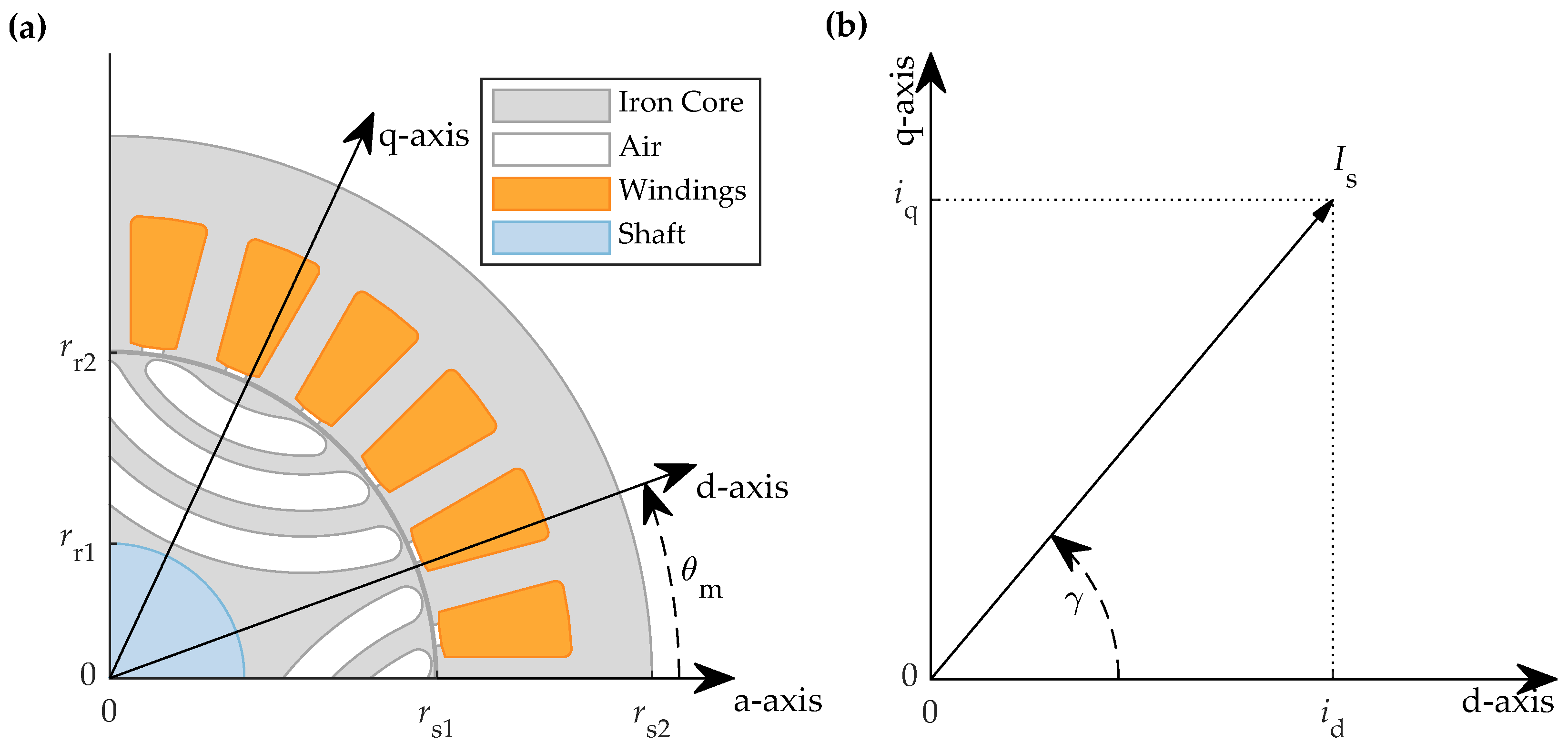
Synchronous machines are typically modeled in the dq rotating reference frame [5,7,12]. The instantaneous total electromagnetic torque, , in these machines is generally a nonlinear function of the stator current components and , influenced by the saturation effects of the stator and rotor iron cores. It also depends on the mechanical rotor position , which is affected by the varying reluctance due to the slots in the stator and rotor iron cores. The mechanical and electrical positions are related by the number of machine pole pairs , such that . For SynRMs, the d-axis is typically aligned with the path of the lowest reluctance in the rotor iron core, as presented in Figure 1a.
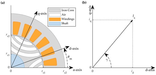
Figure 1.
(a) Schematic representation of a 4-pole () SynRM. (b) Depiction of a current vector in the dq reference frame, showing its components and , as well as its polar form with amplitude and angle .
The magnetic flux linkages in the d- and q-axes, and , represent the average flux linkages with respect to the rotor position and are thus independent of . In contrast, is the magnetic co-energy, which depends on the stator current components and , as well as the rotor position . The variation of with respect to corresponds to the torque ripple , whose average value over a full rotor rotation is zero. Therefore, this term is omitted when analyzing the generated instantaneous average torque [5].
It is important to note that and are nonlinear due to the magnetic saturation effects of the stator and rotor iron cores. The degree of nonlinearity depends on the machine type (e.g., SynRM, PM-assisted SynRM, surface or interior PM synchronous machine) and design (e.g., distributed or concentrated windings, geometry and size of the machine, air gap between stator and rotor, etc.).
In SynRMs, there are no PMs, so both flux linkages are produced solely by the current components and and can be expressed in terms of the apparent inductance by (2),
and in terms of the apparent inductance by (3).
Both and are inherently nonlinear functions of the current components and . By incorporating (2) and (3) into (1), and neglecting the torque ripple , the instantaneous average torque can be expressed by (4),
where is the difference between the apparent inductances in the d- and q-axes [5]. The total average torque in SynRMs is due solely to the reluctance torque, which arises from the interaction between the magnetically salient rotor (i.e., varying reluctance) and the magnetic field generated by the stator current. The orientation adopted in Figure 1a results in and . For motor operation, this requires the product to be positive, while for generator operation it must be negative. Achieving attractive performance characteristics relies heavily on the design of air gaps in magnetic paths of the d- and q-axes. The performance of SynRMs is not competitive if the saliency ratio, defined as the ratio between and , is below 7. This ratio is also reflected in the inductance difference . To attain such a saliency ratio, at least three adequate flux barriers in the q-axis are required, along with the smallest possible air gap between the stator and rotor in the d-axis, as illustrated in Figure 1a. Flux barriers generally increase the effective air gap, thereby decreasing and linearizing the inductance . Conversely, minimizing the air gap in the d-axis allows for high inductance , which behaves highly nonlinearly due to the iron core saturation. For further details on the impact of design on performance, nonlinear properties, and control, refer to [4,5,7].
In the field of motor control, (4) is often expressed in terms of the current vector in polar coordinates, defined by its amplitude and angle , as presented in Figure 1b. The main reasons are, e.g., as follows:
- The vector amplitude corresponds directly to the amplitude of the phase currents in the stator windings due to the application of amplitude invariant transformation;
- The conduction power loss is proportional to ;
- The speed controller typically provides the amplitude of the stator current as the basis for determining reference values for the current controllers.
2.2. Conduction Power Loss Optimization Control Strategy
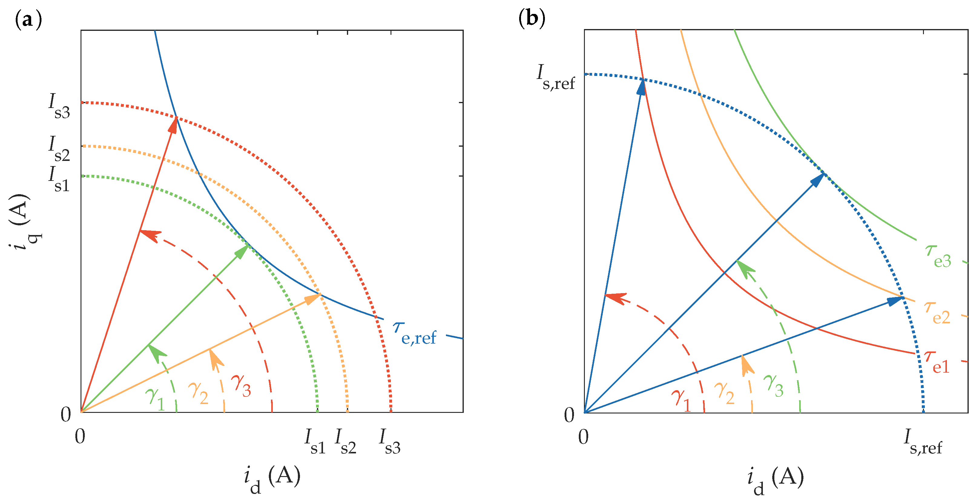
The nature of electromechanical energy conversion in the discussed machines, as summarized in (4) or (9), allows for generating a desired torque within the machine’s physical constraints using two degrees of freedom, namely, by adjusting and/or [19,20]. Thus, the reference torque can, theoretically, be achieved by an infinite number of combinations of (or, equivalently, ), as shown schematically in Figure 2a.
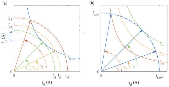
Figure 2.
There are two viewpoints when optimizing conduction power loss: (a) A reference torque can be generated by various combinations of . The combination represents the minimum possible current amplitude for , making it the optimal combination. (b) A reference current can generate various torques depending on the applied angle . The torque is the maximum achievable torque for , so the combination is optimal.
To enhance energy efficiency and performance limits during machine operation, the most common control strategy is to minimize the conduction power loss in the stator windings, [19,20]. Since is proportional to , optimal operation requires minimizing for a given .
From another perspective, a reference amplitude of the stator current can result in various output torques when different angles are applied, as shown schematically in Figure 2b. Similarly to the first perspective, the energy efficiency and performance limits during machine operation are maximized when the generated torque for a given is maximized.
Both approaches lead theoretically to the same result, known commonly as maximum torque per ampere (MTPA) operation. This term is derived from the second perspective, while a more general and appropriate term is maximum torque per current operation, though it is used less frequently in practice [19,20]. Considering the first perspective of the control strategy, a straightforward term could be minimum current for a desired torque strategy. Regardless of the terminology, and despite both approaches leading to the same reference trajectory in the dq-reference plane, the distinction is important when implementing the MTPA control strategy in applied engineering [19,20].
This strategy is used typically in conjunction with FOC techniques. In FOC, the current components and are controlled by separate proportional–integral (PI) controllers in the dq rotating reference frame to generate the desired torque output. The MTPA strategy is generally integrated into FOC to provide the optimal current references and for a desired operating point. The operating point is defined by a single control (input) variable, provided either directly by the user or by a master controller (e.g., typically a speed controller) in cascaded control schemes. This input variable can be either the torque reference or the current reference , depending on the implemented FOC scheme [19,20]. Therefore, we can distinguish between two general implementation schemes, which are discussed below.
2.2.1. Minimum Current for a Reference Torque
When the reference variable is , the optimal operating condition is achieved by applying the smallest possible current , with the current angle adjusted adequately, as shown in Figure 2a. The optimal operating condition for a given is determined by a unique combination . This optimal combination can be found by solving the nonlinear optimization problem (10):
where is the maximum amplitude of the stator current, which is usually limited by thermal or demagnetization aspects or limited by the power supply. The so-called MTPA trajectory (or curve) is obtained by solving (10) for all feasible values [19,20]. This results in a set of optimal polar combinations and corresponding combinations in the dq-reference frame, which are used as reference values for the current controllers in FOC.
2.2.2. Maximum Torque for a Reference Current
When the reference variable is , the optimal operating condition is achieved by adjusting the current angle to maximize the generated torque . The optimal operating condition for a given corresponds to a unique combination . This optimal combination can be determined by solving the nonlinear optimization problem (11).
The corresponding MTPA trajectory is constructed from all feasible combinations of or the corresponding in the dq-reference frame [19,20]. These are used directly as reference values for the current controllers in FOC.
It is important to note that both approaches rely on the nonlinear map , which can be obtained for a specific machine either numerically or experimentally.
2.3. Estimation and Implementation of the MTPA Strategy in Control Schemes
The implementation of the MTPA strategy can be categorized further based on how the reference currents and are obtained and updated, with both offline and online methods being applicable [19,20]. Offline methods rely on analytical or numerical estimation of the trajectories prior to the operation of the drive. In contrast, online methods estimate MTPA operation in real time by analyzing the variables obtained during the drive’s operation. This research focused solely on the offline approach.
The MTPA trajectories can be estimated either analytically or numerically [19,20,32]. By applying the MTPA conditions and to (9), both nonlinear and linear flux–current MTPA formulations can be derived analytically.
In the simpler case of a linear flux–current relationship, the apparent inductance difference is considered constant. However, the resulting MTPA condition can lead to significant deviations from the actual optimal operating conditions [19,20].
The nonlinear flux–current MTPA formulation can be obtained analytically in an implicit form [19,20]. This approach is significantly more complex to derive, solve, and implement in real-world engineering applications compared to the constant parameter formulation. Consequently, it is used rarely in practice. It is important to note, however, that the nonlinear formulation implies that not only the apparent inductances but also the differential inductances (i.e., the local changes in inductances with respect to and ) affect the shape of the MTPA trajectories [19,20]. In engineering applications, analytic formulations for approximating MTPA trajectories are often replaced by LookUp Tables (LUTs) or various mathematical functions. These are determined using numerical methods based on a calculated or measured nonlinear map for a specific SynRM.
3. Analysis of Suboptimal Operation
Suboptimal MTPA operation occurs when the instantaneous values of current amplitude and angle do not correspond to the theoretically optimum MTPA trajectory, as presented in Figure 2. As a consequence, the torque-to-current ratio is not the highest possible for a specific operating point and could be increased by either correcting the current amplitude and angle if is the input or by correcting the current angle if the current amplitude is the input. Such operation is, to some extent, always occurring during transients, even if the steady-state operating point is on the MTPA trajectory. However, suboptimal MTPA operation often also occurrs in steady state. The obvious source for such operation is an inaccurately determined MTPA trajectory, providing erroneous references to the current controllers. Further, other factors, such as misalignment of the reference frame (in both sensor and sensorless applications) and inaccuracy of current sensors, lead to suboptimal MTPA operation.
3.1. Methodology
The analysis of suboptimal MTPA operation concerning angle errors was performed for both discussed control implementation approaches and for both assumed linear and nonlinear magnetic properties of SynRMs. The linear case was analyzed analytically, while the nonlinear case was analyzed numerically.
In both the discussed control implementation approaches (i.e., where the input variable was either torque or current amplitude ), it is crucial to determine the optimal current angle accurately, as detailed in Section 2.2. Consequently, the presented analysis is based on the variation of the current angle around the optimal angle . By introducing the angle deviation , the actual angle is defined by (12)
where, in the case of , an overestimated suboptimal angle is considered, and, in the case of , an underestimated suboptimal angle is considered.
In the analysis, two key performance indicators (KPIs) were evaluated with respect to . The first KPI assessed the normalized deviation of conduction power loss under suboptimal operating conditions. Therefore, the ratio between the squares of the suboptimal current and the corresponding optimal current was defined by (13).
This KPI was defined to assess the suboptimal operating conditions if the input (master) control variable was assumed , where, by definition, .
The second KPI was defined as the ratio between the suboptimal torque and the corresponding optimum value , as defined by (14).
This ratio enabled analysis of the normalized deviation of the suboptimal torque with respect to the error in current angle if the input (master) control variable was assumed , where, by definition, .
3.2. Analytical Evaluation Assuming a Linear Flux–Current Relationship
Assuming a linear flux–current relationship, the apparent inductances and , as well as their difference , are constant. Consequently, for a desired stator current , the generated torque is defined by (15).
A SynRM can achieve a desired torque with various combinations of , as described in Section 2.2, regardless of the assumption of linear properties. For a given , the corresponding can be determined by (16).
From both (15) and (16), it is straightforward to determine the optimum current angle , which, in this case, is independent of the operating point (i.e., or ) and is defined by (17).
By considering (17) in (15) and (16), the optimum torque for a reference current is defined by (18),
whereas the square of optimum current for a reference torque is defined by (19).
Both KPIs (13) and (14) were determined based on obtained analytic functions (15) to (19). The power-loss increase KPI with respect to the angle error is defined by (20),
where is considered in (16).
Analogously, the torque decrease KPI with respect to the angle error is defined by (21),
where is considered in (15).
The obtained results, (20) and (21), indicate that both the normalized torque decrease and the normalized power-loss increase due to the angle error are independent of the operating point. They remain constant across all operating conditions (i.e., for all feasible control inputs or ) if a constant angle error is assumed. With respect to , both deviations are related to a cosine function of the double error angle, which has the lowest gradients around the optimum angle where . This implies that the sensitivity to performance decrease is lowest near the optimum angle and increases with increasing . Finally, the relation between the performance decrease KPIs and is defined by (22),
where the term is eliminated by considering (20) and (21). This result suggests that SynRMs are more sensitive to power-loss increase compared to torque decrease with respect to .
The relationships obtained in (20) and (21) can also be used to define the angle error range corresponding to an acceptable maximum performance decrease KPI. For a given acceptable maximum power-loss increase ratio, , the corresponding error angle limit, , is defined by (23).
All angle deviations, , that are equal or smaller than the obtained error angle limit (i.e., ) result in , indicating an acceptable power-loss increase. Consequently, the corresponding acceptable angle error range is defined between the limit for overestimated angles, , and the limit for underestimated angles, .
Analogously, an error angle limit, , corresponding to a given acceptable minimum torque decrease ratio, , is defined by (24).
All angle deviations, , that are equal or smaller than the obtained error angle limit (i.e., ) result in , indicating an acceptable torque decrease. Consequently, the corresponding acceptable angle error range is defined between the limit for overestimated angles, , and the limit for underestimated angles, .
It is important to note that the performance decrease, in both cases, is symmetric with regard to over- or underestimation of the optimum angle .
3.3. Numerical Evaluation Assuming a Nonlinear Flux–Current Relationship
The functions , , and are highly nonlinear and difficult to express analytically. Consequently, modern approaches use primarily numerical methods, with data derived from contemporary FEM models or from adequate measurements.
In the nonlinear case, the power-loss increase KPI depends on both the angle error and the reference torque . It can be determined numerically by solving the nonlinear optimization problem (11), then calculating the increased current amplitudes for various at , and applying these values to (13).
The angle deviation limit for an acceptable power-loss increase ratio can be found by using (25),
where is, in general, not symmetric around . The deviation limit for underestimated angles can be obtained by assuming and , whereas the deviation limit for overestimated angles can be obtained by assuming and .
Similarly, the torque decrease KPI depends on both the angle error and the reference current amplitude . It can be determined numerically by solving the nonlinear optimization problem (10), then calculating the decreased torques from the torque map , and applying these values to (14).
The deviation limit with respect to an acceptable torque decrease ratio can be obtained by solving (26),
where is, in general, not symmetric around . The deviation limit for underestimated angles can be obtained by assuming and , whereas the deviation limit for overestimated angles can be obtained by assuming and .
4. Results
The numerical analysis was conducted using Matlab, based on the open-source software package named Synchronous Reluctance—evolution (SyR-e) [4,37], version 3.8.1, which is available on GitHub and also through the Matlab file exchange platform. SyR-e, developed in Matlab/Octave, facilitates the open-source design, optimization, and analysis of various types of electric machines. It utilizes the open-source software package Finite Element Method Magnetics (FEMM), version 4.2, for electromagnetic FEM numerical analysis. The main reasons for using SyR-e in this research were:
- The presented numerical analysis can be performed with free open-source software (Matlab can be substituted with GNU Octave);
- SyR-e provides template designs for several machine types;
- The available template SynRM design has been manufactured, tested, and validated experimentally by the authors of the package [4,13].
- In this research, SyR-e was used to generate numerical data (i.e., torque and flux linkage maps , , and ) for a selected template SynRM. The gathered data were saved and analyzed further in Matlab 2023b according to the presented methodology. The numerical analysis was performed on a standard desktop computer. This approach allows all interested researchers to replicate and expand upon the presented research.
4.1. Design of the Analyzed Synchronous Reluctance Machine
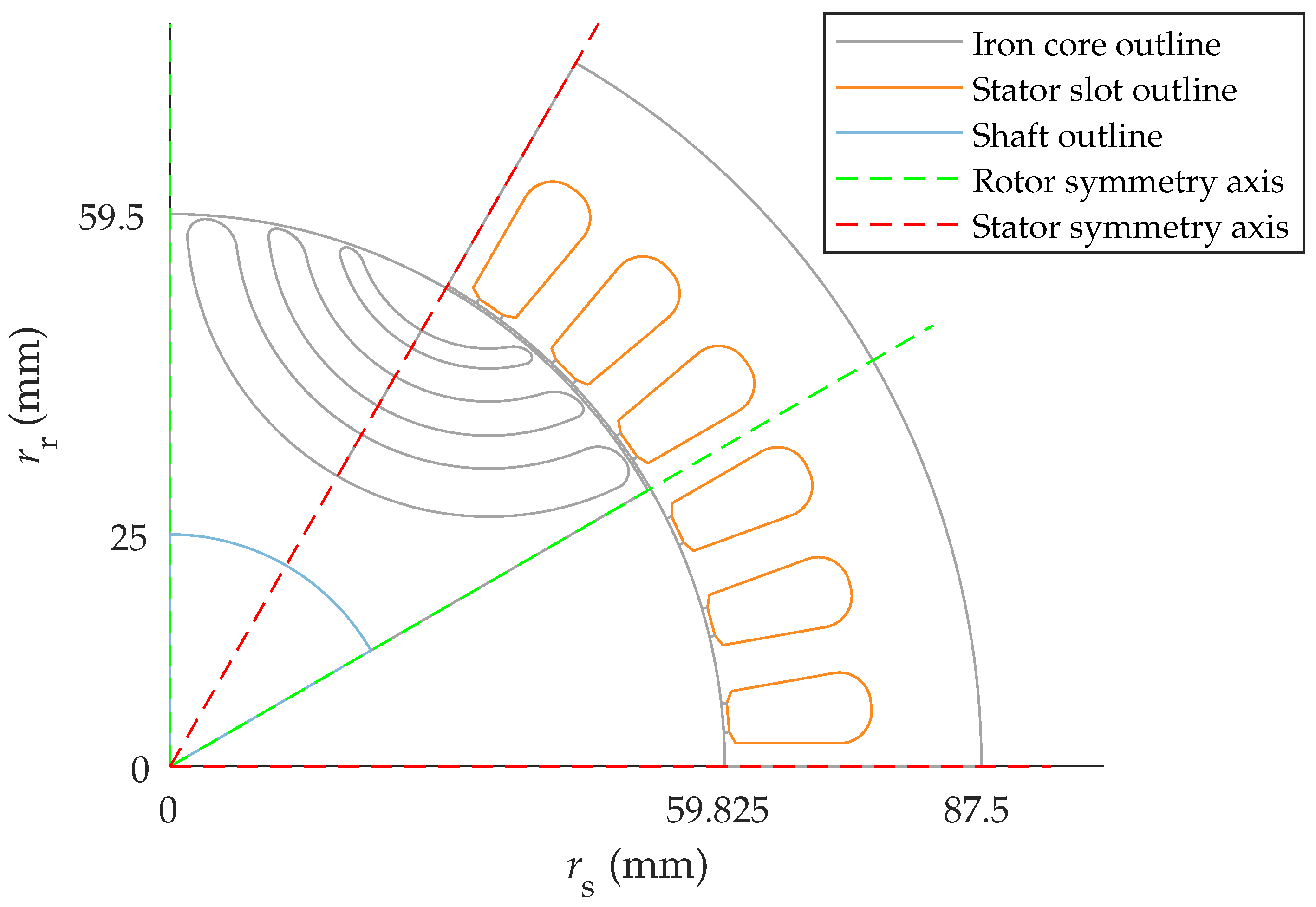
The selected case study machine is a six-pole, three-phase SynRM with 36 stator slots and three rotor barriers. The rotor was originally designed and optimized to retrofit an induction machine stator [4,13]. It was designed and manufactured in collaboration between Politecnico di Torino, Università di Modena e Reggio Emilia and the company Raw Power s.r.l.; hence, it is denoted by the name RAWP. It can be selected, modified, and analyzed within SyR-e. The geometry of the machine, including the corresponding rotor and stator radii, and , is presented in Figure 3. All the design parameters adhered to the default RAWP template values, including the material properties.
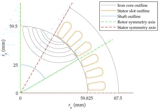
Figure 3.
The geometry of the analyzed RAWP SynRM, featuring 6 magnetic poles, allows for the simplification of modeling only of the entire geometry in the FEM analysis.
4.2. Numerical Evaluation of the Nonlinear Properties
The nonlinear maps of the discussed machine were obtained using the Flux Maps evaluation feature in SyR-e. The flux and torque maps were computed over a defined regular domain in FEMM with a static magnetic solver. The evaluation domain was defined with four quadrants (), a calculated maximum current amplitude of A, and 129 current levels for evaluation () for both the d- and q-axes. This resulted in an evaluation resolution of approximately A, producing numeric maps with elements for each quadrant. The analysis focused on motoring operation, considering only the first quadrant of the obtained maps.
4.2.1. Flux Linkage Maps
The calculated nonlinear map of the analyzed RAWP SynRM is presented in Figure 4. The corresponding map is presented in Figure 5.
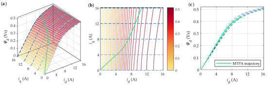
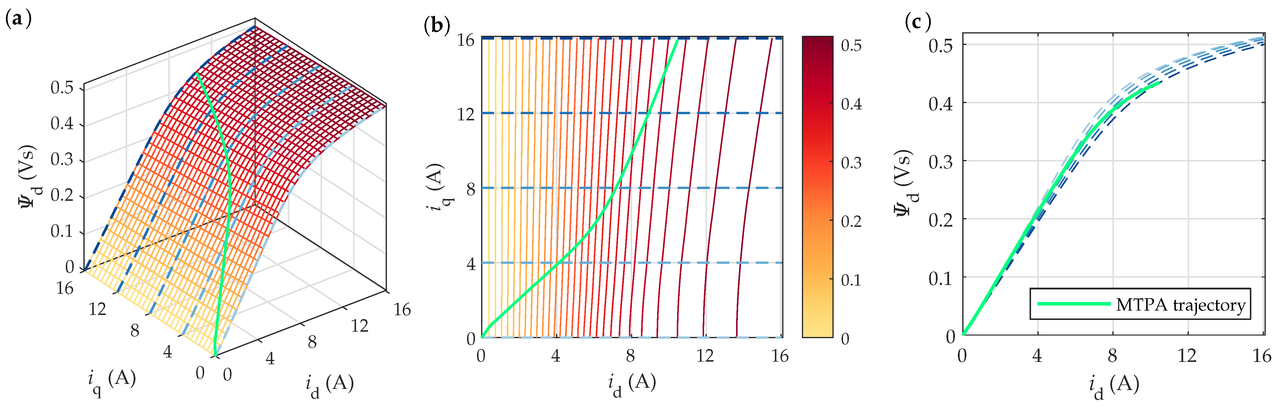
Figure 4.
Flux linkage map of the analyzed RAWP SynRM, with the MTPA trajectory highlighted: (a) 3D view; (b) contour view with isolines; (c) parametric view for selected values of .
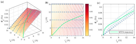
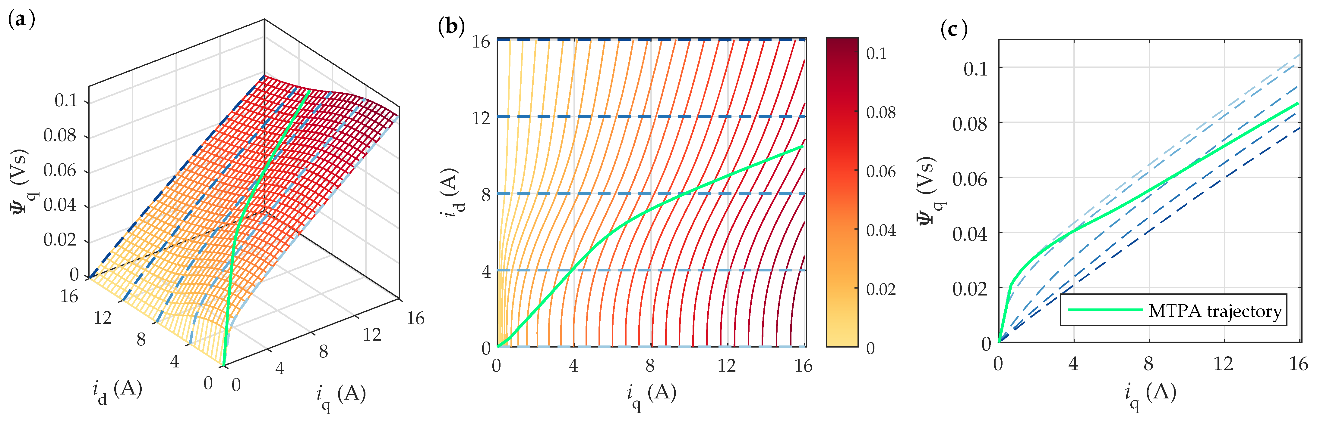
Figure 5.
Flux linkage map of the analyzed RAWP SynRM, with the MTPA trajectory highlighted: (a) 3D view; (b) contour view with isolines; (c) parametric view for selected values of .
The flux linkage in the d-axis (i.e., the axis of the lowest reluctance) was impacted predominantly by the current component , where, at approximately A, the magnetic paths started to saturate. Due to saturation, the MTPA trajectory deviated from the theoretically ideal linear MTPA angle and curved towards the q-axis, which is a common property of SynRMs [5,7].
The flux linkage in the q-axis (the axis of highest reluctance) was influenced predominantly by the current component . Due to additional flux barriers in the magnetic circuit, this flux linkage was significantly lower and increased more linearly within the evaluated region compared to . In the subregion where A, the effect of unsaturated iron bridges between the flux barriers was clearly pronounced for A. When A, these bridges became saturated, and the relationship was almost linear. It is important to note that these barrier bridges could be saturated by both and individually. Along the MTPA trajectory, was saturated predominantly by at approximately A and was almost linear for A. Due to these effects, the MTPA trajectory curved towards the q-axis at A. However, when the flux barrier bridges were saturated, the MTPA trajectory curved back to the theoretically ideal linear MTPA angle .
4.2.2. Inductance Maps
The nonlinear inductance maps, presented in Figure 6, were calculated based on the flux linkage maps in Figure 4 and Figure 5. The obtained apparent inductance maps, in Figure 6a and in Figure 6b, resembled the corresponding incremental inductance maps in Figure 6d and in Figure 6e.
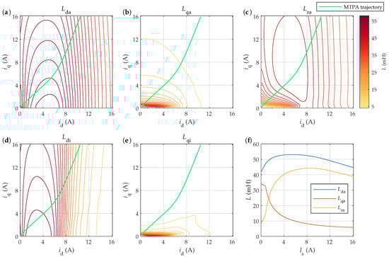
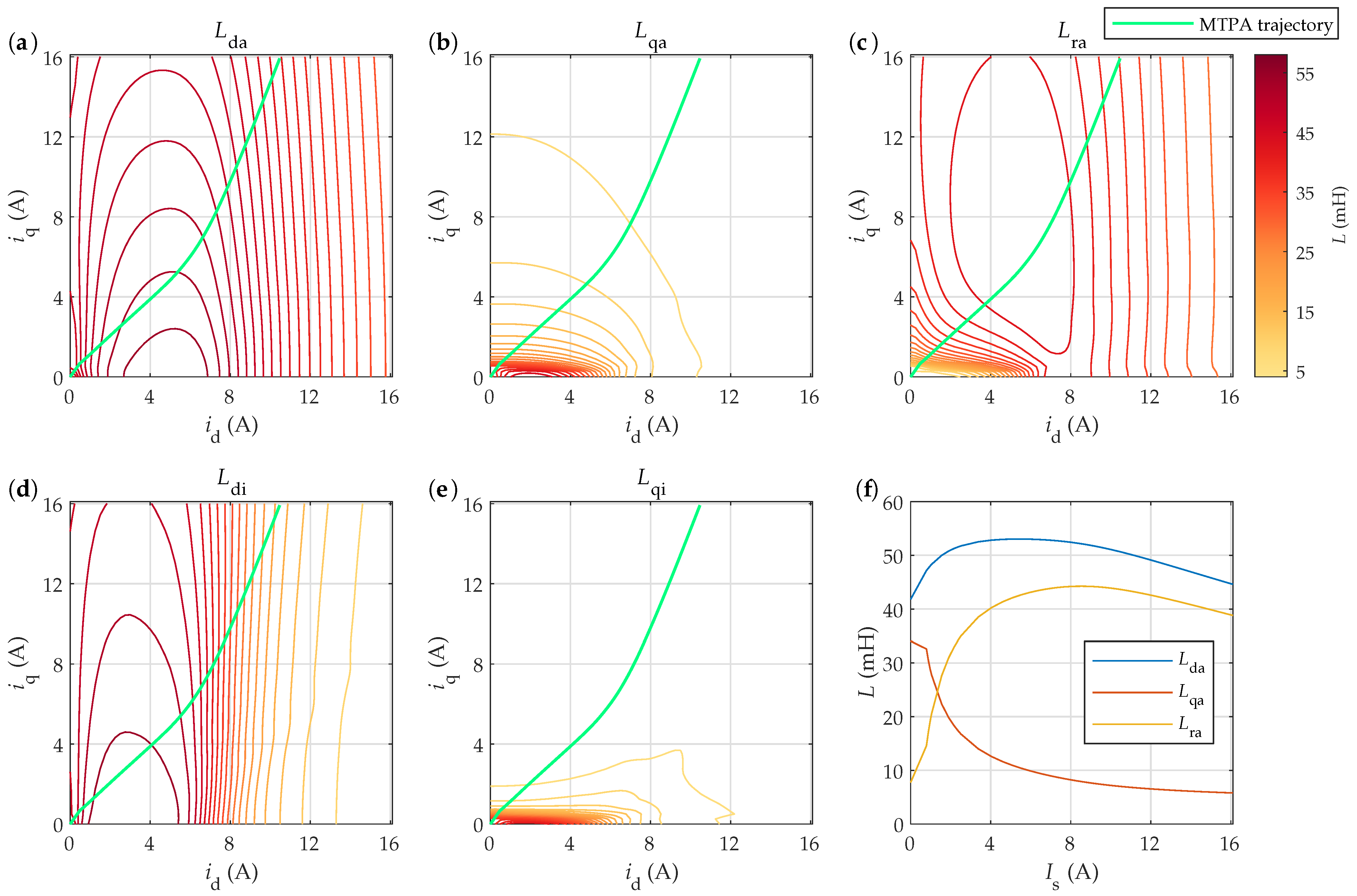
Figure 6.
Inductance maps of the analyzed RAWP SynRM, with the MTPA trajectory highlighted: (a) contour view of the apparent inductance ; (b) contour view of the apparent inductance ; (c) contour view of the difference in apparent inductances ; (d) contour view of the incremental inductance ; (e) contour view of the apparent inductance ; (f) apparent inductances , , and with respect to along the MTPA trajectory.
The apparent inductance maps have, in general, lower gradients compared to their respective incremental inductance maps because the determination of apparent inductances is based on (2) and (3), which smoothens the nonlinearity of the corresponding flux linkage maps. The average torque is, according to (4), dependent only on the difference , which is presented in Figure 6c. Finally, the obtained relationships of apparent inductances , , and with respect to the current amplitude along the MTPA trajectory in Figure 6f confirmed that the unsaturated rotor barrier bridges reduced the torque-to-current ratio (which is proportional to ) significantly, whereas the saturation of the d-axis magnetic path did not reduce this ratio as heavily because both apparent inductances were reduced approximately evenly at higher currents . It is, further, important to note that the shape of does not reflect the shape of the obtained MTPA trajectory directly, which relates more to the discussed nonlinearity in and .
4.2.3. Torque Maps and MTPA Trajectories
Based on the presented results, the nonlinear SynRM model was approximated using a simplified SynRM model with a linear flux–current relationship, assuming constant apparent inductances. The inductance was chosen to approximate the nonlinear over a wide range of . We selected mH, which, effectively, approximated the range from A to A, as shown in Figure 6f. This selection resulted in models with equal torque-to-current ratios at approximately A and A. The simplified model was used as the baseline for comparison to assess the impact of saturation in the analyzed SynRM. The resulting torque maps are presented in Figure 7. The maps in Figure 7a,b were calculated based on (4). The torque map for the SynRM model with a linear flux–current relationship is presented in Figure 7a. In Figure 7b, the torque map for the SynRM model with a nonlinear flux–current relationship is presented, which was calculated based on the nonlinear map , shown in Figure 6c.
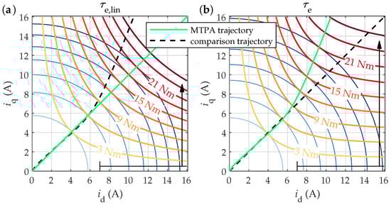
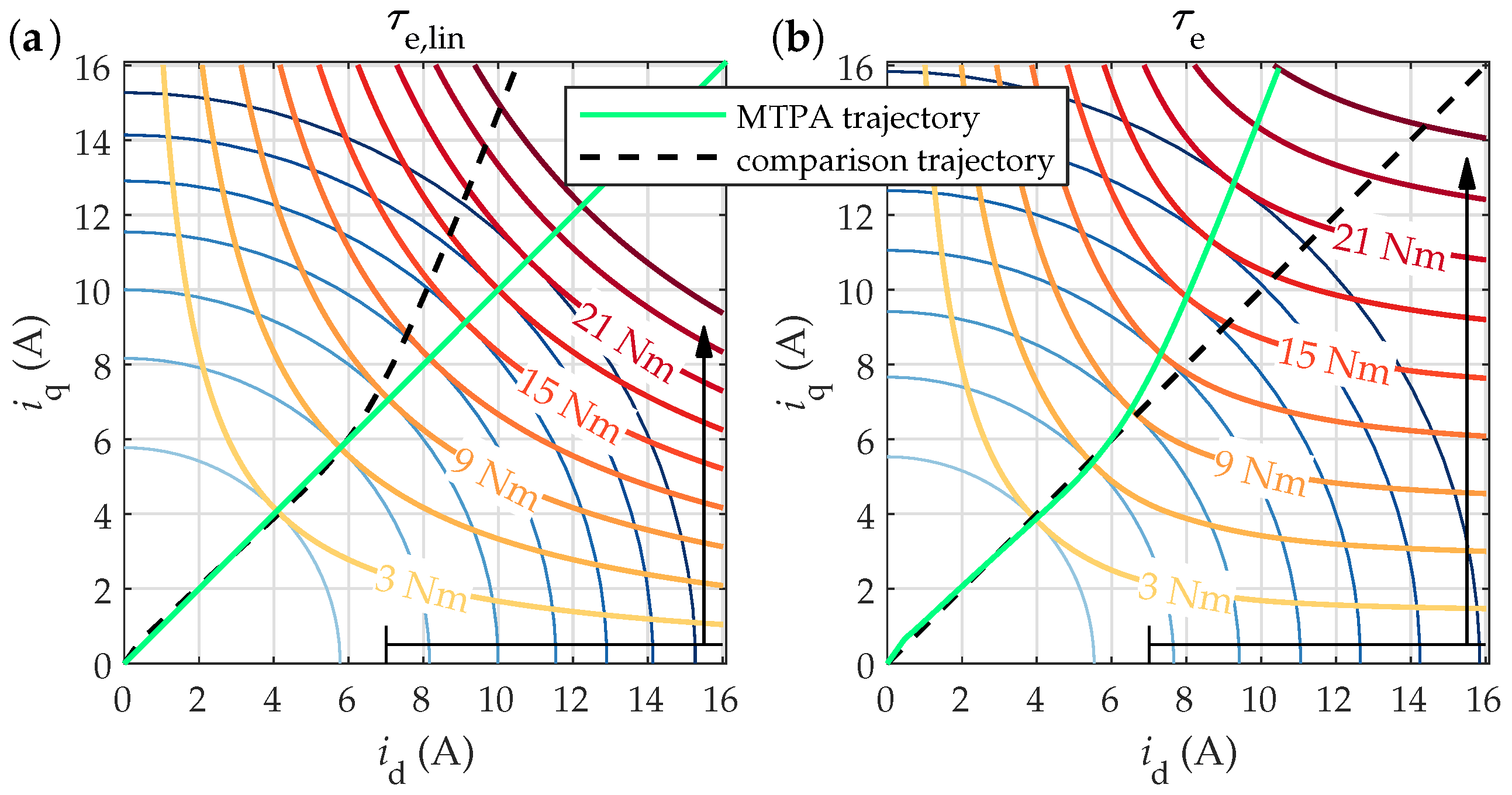
Figure 7.
Torque maps of the analyzed RAWP SynRM, with the MTPA trajectories highlighted: (a) contour view of for the simplified model with linear material properties; (b) contour view of for the model with nonlinear material properties.
Further, the MTPA trajectories were determined numerically. These can be determined numerically by solving either (10) or (11), depending on whether the input variable is or . In the presented case, the trajectories were determined by solving (10), which enabled the straightforward addition of circular isolines of optimum stator current amplitudes that corresponded to the presented isolines of torque .
The impact of saturation on the generated average torque was evaluated by comparing the determined maps. The most significant effect was due to the saturation of the magnetic path along the d-axis, resulting in a sparser distribution of isotorque lines along the q-axis in the region where A. This is schematically indicated by the longer arrow in Figure 7b compared to the corresponding arrow in Figure 7a. The asymmetric deformation of the torque map increased the curvature of the isotorque lines, causing the nearest point on the corresponding contours to the reference frame origin (i.e., the point of contact between the observed torque contour and the corresponding MTPA current amplitude circle) to shift closer to the q-axis, as shown in Figure 7b. Consequently, the MTPA trajectory curved towards the q-axis, which is a direct result of the nonlinearity of apparent and incremental inductances, as discussed in Section 2.3. In contrast to this, the MTPA trajectory in the linear case is a straight line with the MTPA current angle .
4.3. Power Loss Increase Due to Angle Errors in Suboptimal Operation
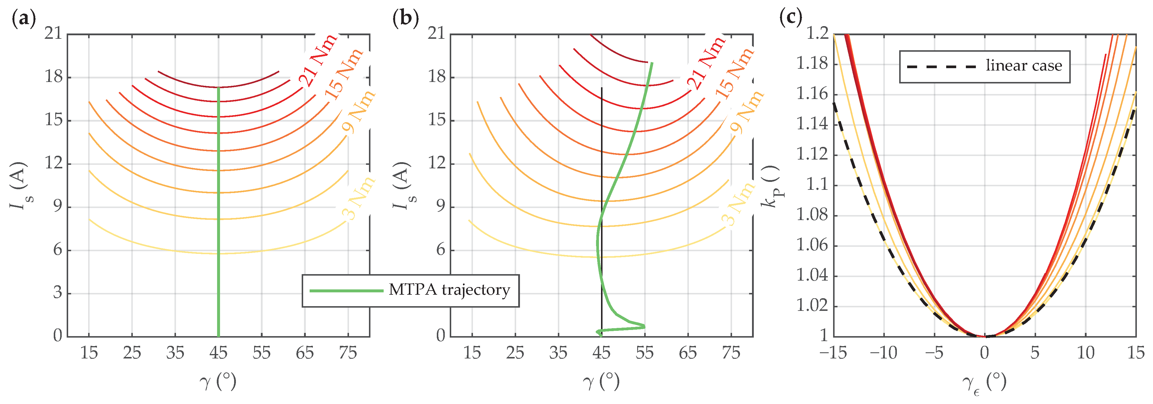
Considering that the reference torque is the control input, any angle deviation results in suboptimal operation of a SynRM, leading to increased power losses compared to MTPA operation, as presented in Figure 2a. This performance decrease was evaluated based on the KPI , defined by (13). This part of the analysis involved transforming the torque maps presented in Figure 7a,b from the coordinates to the coordinates . The corresponding transformed maps are presented in Figure 8a,b. In the reference frame, the optimum stator current vector is defined by , which corresponds to the point of minimum for a given reference torque. This is intuitive and straightforward to recognize from the obtained results. The map for the linear case in Figure 8a corresponds to the square root of (16), where mH and were considered. The current increases symmetrically around the minimum values for all , with all minimum values of current occurring at .
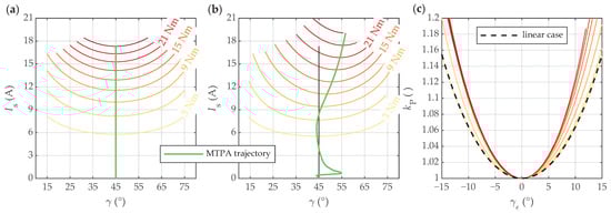
Figure 8.
Torque maps of the analyzed RAWP SynRM, with the MTPA trajectories highlighted: (a) contour view of for the simplified model with linear material properties; (b) contour view of for the model with nonlinear material properties; (c) normalized increase in conduction power loss as a function of angle deviation for the linear case (dashed line) and for the nonlinear case (solid lines, color-coded to isotorque lines in subplot (b)).
The map for the nonlinear case in Figure 8b was obtained numerically, based on the map in Figure 7b. Compared to the linear case, the obtained torque isolines were more curved around the optimum values with a sparser distribution, which was a direct consequence of saturation of the magnetic path in the d-axis. Furthermore, saturation in both the d- and q-axes resulted in the shift of optimum angles , predominantly towards higher values compared to the linear case, which was also reflected in the nonlinear shape of the MTPA trajectory in the dq-reference frame, as discussed in Section 4.2.3.
By evaluating both discussed maps with (13), the power-loss increase KPI was determined and analyzed numerically. The obtained results are presented in Figure 8c. In the linear case, the numerically obtained for all the isotorque lines aligned perfectly with analytically obtained results into a signle curve, defined by (20). The curve, presented with the dashed line, confirmed that was independent of . In the nonlinear case, saturation of the magnetic path in the d-axis caused a more pronounced asymmetrical increase in conduction power loss with respect to . The obtained , presented with the solid lines in Figure 8c, was dependent on both and , where the presented lines correspond to individual isotorque lines of equal color in Figure 8b.
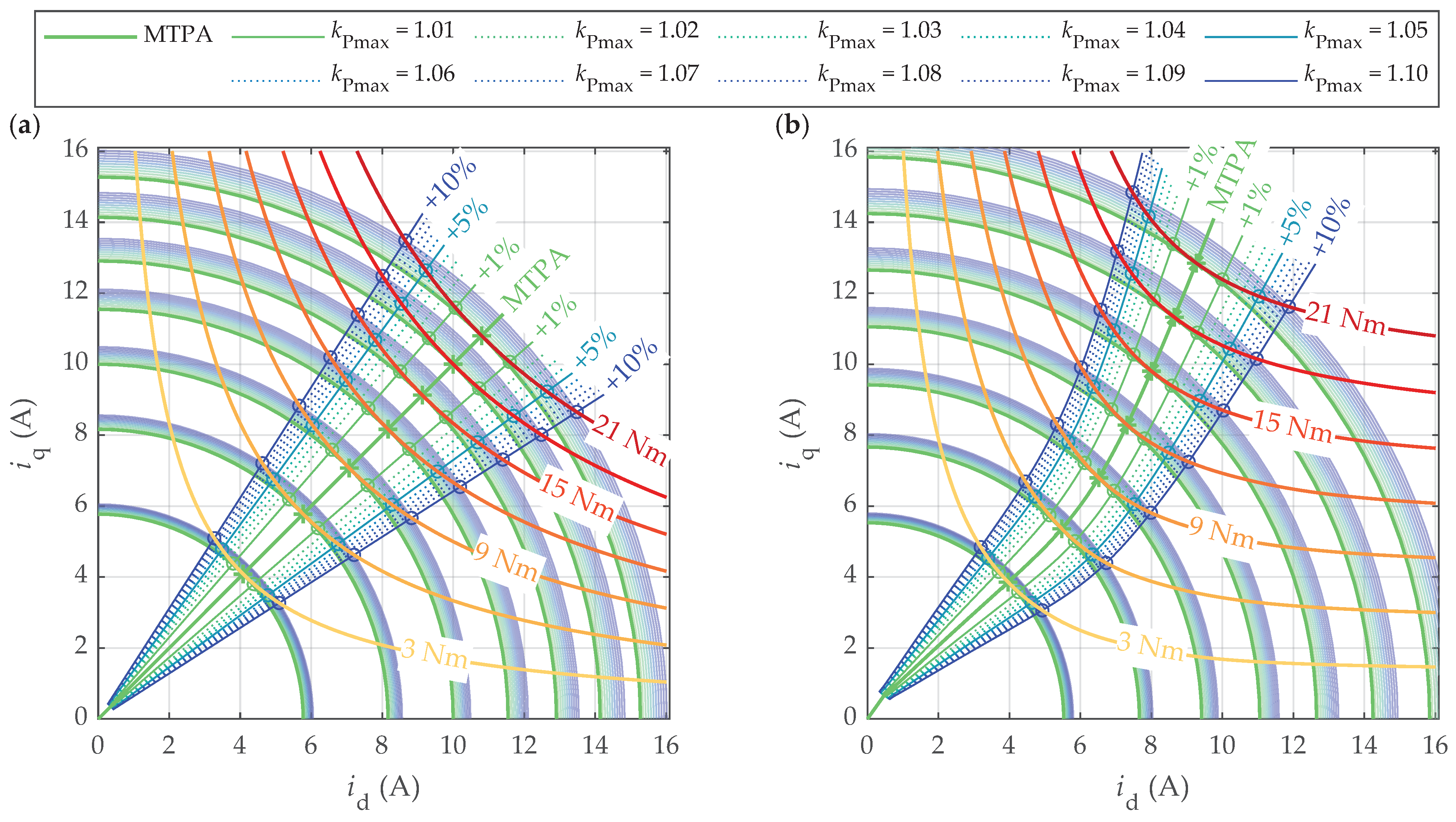
Furthermore, the angle deviation limits and with respect to were determined numerically by solving (25). This analysis was confined to a power-loss increase of up to 10%, i.e., from to . The results obtained within the dq-reference frame are presented in Figure 9.
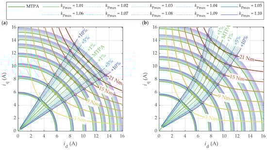
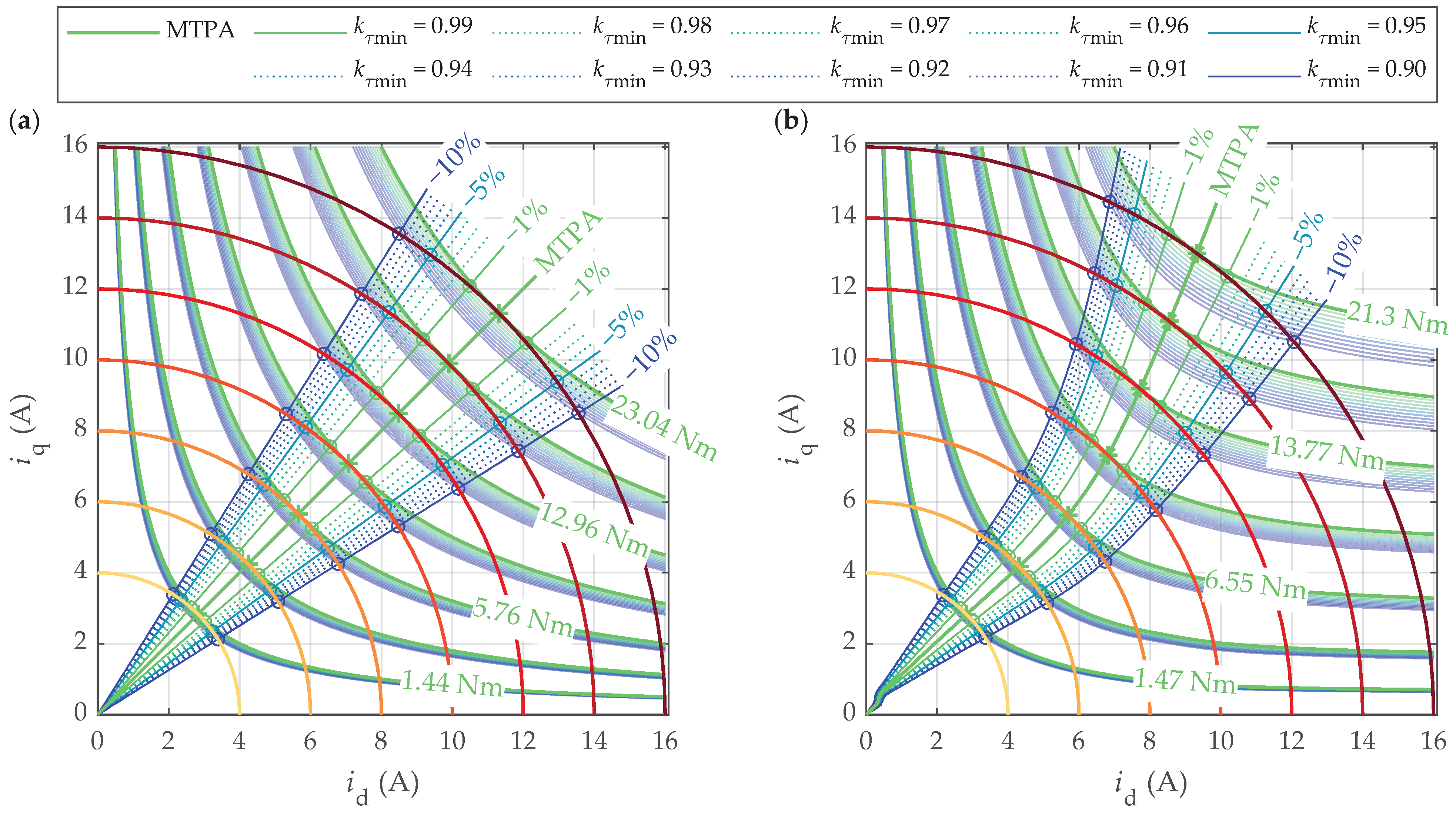
Figure 9.
Angle deviation limit trajectories and for different limit power-loss increase ratios in the dq-reference frame: (a) simplified RAWP SynRM model with linear material properties; (b) RAWP SynRM model with nonlinear material properties. The color-coded circular isolines correspond to stator current amplitudes for all the presented combinations of and .
The results confirmed that the sensitivity to suboptimal operation was the lowest in close proximity to the MTPA trajectories and increased with angle deviations in both the analyzed cases. The limit trajectories and followed the corresponding MTPA trajectory in both the linear case, presented in Figure 9a, as well as in the nonlinear case, presented in Figure 9b. In the linear case, the obtained limit trajectories were linear and symmetric around the MTPA trajectory. In contrast to this, in the nonlinear case, these trajectories were nonlinear and asymmetric with respect to the under- and overestimated angles.
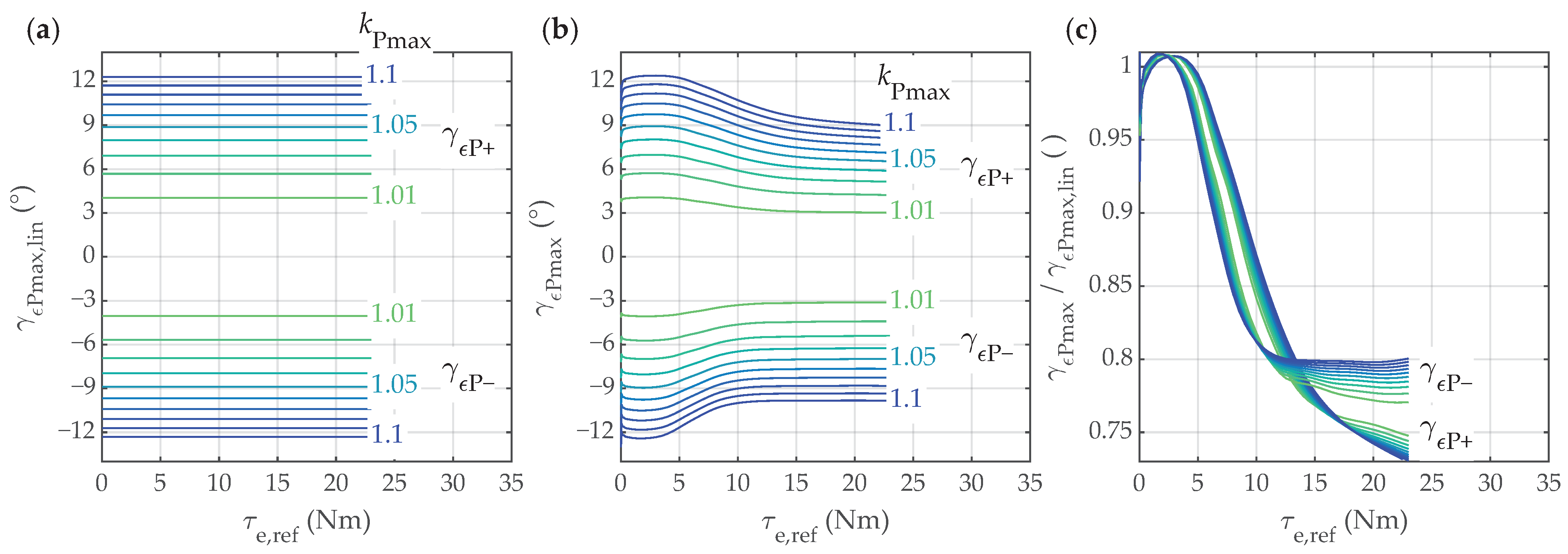
The impact of saturation was finally investigated by analyzing the relationship of the angle deviation limits and with respect to and . The results are presented in Figure 10.
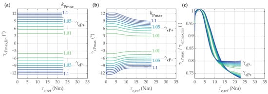
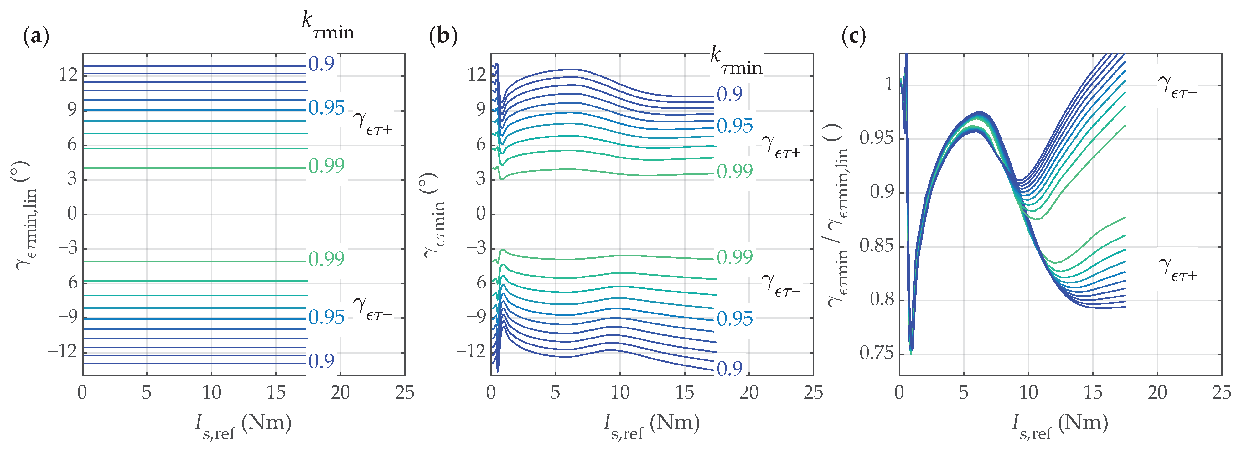
Figure 10.
Parametric plot of the angle deviation limits for : (a) simplified RAWP SynRM model with linear material properties; (b) RAWP SynRM model with nonlinear material properties; (c) ratio between and .
In the linear case, the limit trajectories were independent of , as presented in Figure 10a, and corresponded to the analytically obtained values defined by (23). The lowest sensitivity to conduction power-loss increase was confirmed in close proximity to the MTPA trajectory. It enabled noticeable deviations in the angle for only a slight increase in power loss. For example, for a maximum 1% increase in power loss (i.e., ), the error in angle could be . The result represented a significant angle error band of width of more than . For a maximum 2% decrease in torque, the error in the angle could be up to , whereas for a maximum 5% decrease in torque, the deviation in the angle could be up to . It is important to note that these results are valid for all SynRMs, regardless of geometry, size, etc., only if a linear flux–current relationship is assumed.
However, magnetic saturation curved the limit trajectories closer to the MTPA trajectory, decreasing the error band, as presented in Figure 10b. Further, the limit trajectories for underestimated angles were deformed at lower compared to trajectories because, at lower angles , the magnetic path of the d-axis is generally more saturated. The impact was assessed finally by calculating the ratio between the obtained in the nonlinear and linear cases. The results are presented in Figure 10c. The obtained scaled nonlinear limit curves were remarkably similar. The nonlinear limit trajectories were from 20% to up to 27% closer to the MTPA trajectory in the saturated condition of the SynRM, reducing the available deviation band accordingly. The allowed angle error band for up to 1% increase in power loss was, however, still noticeable, and corresponded to approximately 6 degrees ( around the MTPA trajectory) in the worst saturation case.
4.4. Torque Decrease Due to Angle Errors in Suboptimal Operation
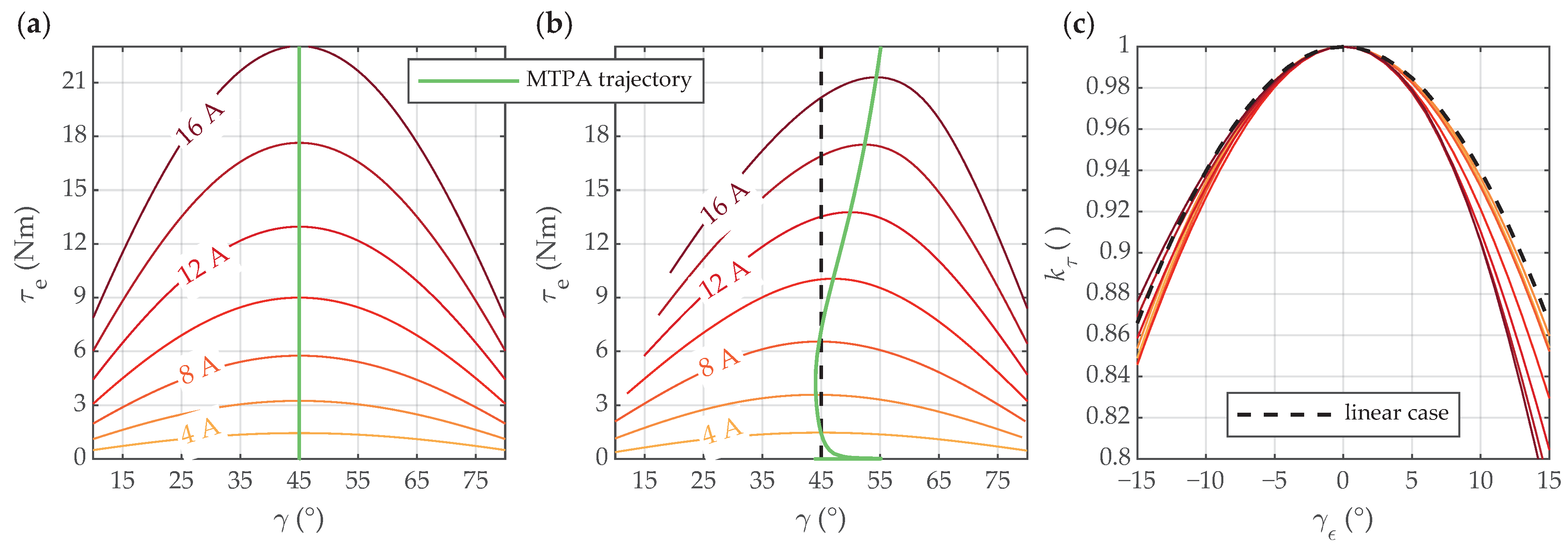
Considering that is the control input, angle errors result in suboptimal operation of a SynRM in terms of a decrease in generated torque compared to MTPA operation, as presented in Figure 2b. This performance decrease was evaluated based on the KPI , which is defined by (14). Analogously to the previous part of the analysis, this part was based on transforming the torque maps presented in Figure 7a,b from the coordinates to current amplitude maps in the coordinates . The corresponding transformed maps are presented in Figure 11a,b.
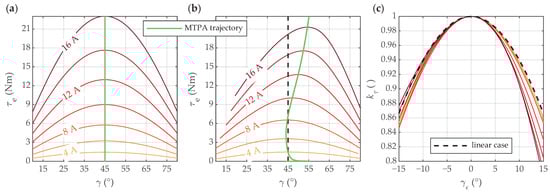
Figure 11.
Stator current maps of the analyzed RAWP SynRM, with the MTPA trajectories highlighted: (a) contour view of for the simplified model with linear material properties; (b) contour view of for the model with nonlinear material properties; (c) normalized decrease in generated torque as a function of angle error for the linear case (dashed line) and for the nonlinear case (solid lines, color-coded to isocurrent lines in subplot (b)).
In the reference frame, the optimum stator current vector is defined by , which corresponds to the point of maximum for a given reference current amplitude . This is intuitive and straightforward to recognize from the obtained results. The map for the linear case in Figure 11a corresponds to (15), where mH and were considered. The torque decreased symmetrically around the maximum values for all , with all maximum values of torque occurring at .
The map for the nonlinear case in Figure 11b was obtained numerically based on the map in Figure 7b. Compared to the linear case, the obtained current amplitude isolines were more curved around the optimum values with a denser distribution, which was a direct consequence of saturation of the magnetic path in the d-axis. Furthermore, saturation in both the d- and q-axes resulted in the shift of optimum angles , predominantly towards higher values compared to the linear case, which is analogous to the results of the previous analysis. It is noteworthy that both discussed approaches to obtain the MTPA trajectory led to the same result.
By evaluating both discussed maps with (14), the torque decrease KPI was determined and analyzed numerically. The obtained results are presented in Figure 11c. In the linear case, the numerically obtained (dashed line) was independent of and aligned perfectly with the analytically obtained results, defined by (21). In the nonlinear case, saturation of the magnetic path in the d-axis caused a more pronounced asymmetrical decrease in generated torque with respect to . The calculated was dependent on both and , which resulted in a family of curves that corresponded to different , as presented with color-coded solid lines in Figure 11c. The obtained results also showed a difference to the results of the analysis of the power-loss increase in the previous section. The difference is that, for underestimated angles, high saturation and , the decrease in generated torque was even slower compared to the linear case, as presented on the left part of the Figure 11c.
Based on (21), the angle deviation limits and with respect to were determined numerically by solving (26). Again, this analysis was confined to a torque decrease of up to 10%, i.e., from to . The obtained results for the dq-reference frame are presented in Figure 12.
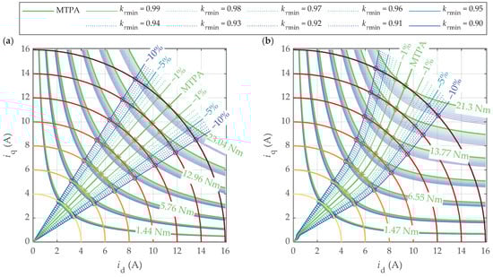
Figure 12.
Angle deviation limit trajectories and for different torque decrease ratios in the dq-reference frame: (a) simplified RAWP SynRM model with linear material properties; (b) RAWP SynRM model with nonlinear material properties. The color-coded reciprocal isolines correspond to torques for all the presented combinations of and .
The obtained results were analogous to the previous analysis and confirmed that the sensitivity to suboptimal operation was the lowest in close proximity to the MTPA trajectories and increased with the increasing angle deviations in both analyzed cases. The limit trajectories and followed the MTPA trajectory in both the linear case, presented in Figure 12a, as well as in the nonlinear case, presented in Figure 12b.
Finally, the impact of saturation was investigated by analyzing the relationship of the angle deviation limits with respect to and . The results are presented in Figure 13.
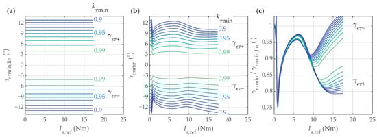
Figure 13.
Parametric plot of the angle deviation limits for : (a) simplified RAWP SynRM model with linear material properties; (b) RAWP SynRM model with nonlinear material properties; (c) ratio between and .
In the linear case, the limit trajectories and were independent of , as presented in Figure 13a, and corresponded to the analytically obtained values defined by (24). The lowest sensitivity of torque decrease was confirmed in close proximity to the MTPA trajectory. It enabled noticeable deviations in the angle for only a slight decrease in the generated torque. For example, for a maximum 1% decrease in torque (i.e., ), the error in the determined angle could be . For a maximum 2% decrease in torque, the error in the angle could be up to , whereas, for a maximum 5% decrease in torque, the deviation in the angle could be up to . The obtained error bands were slightly wider than in the power-loss increase case, which was also derived analytically in Section 3.2. Again, these results are also valid for all SynRMs, regardless of geometry, size, etc., only if a linear flux–current relationship is assumed.
The magnetic saturation curved the limit trajectories closer to the MTPA trajectory for the overestimated angles and also in some operating conditions further from the MTPA trajectory for the underestimated angles, as presented in Figure 10b. The impact was assessed finally by calculating the ratio between the obtained in the nonlinear and linear cases. The results are presented in Figure 13c, where the nonlinear limit trajectories were up to 25% closer to the MTPA trajectory in the saturated condition of the SynRM. In this case, the saturation of the flux barrier bridges also impacted the limit angles at the corresponding current amplitudes. The allowed angle error band for up to 1% decrease in torque was still significant, however, and corresponded to more than 6 degrees (more than degrees around the MTPA trajectory) in the worst case, which is a slightly wider band compared to the corresponding control implementation with .
5. Conclusions
The presented results confirmed that SynRMs exhibit a moderate performance decrease sensitivity to angle errors in MTPA control despite their highly nonlinear magnetic properties. This sensitivity is particularly low near the MTPA trajectory, allowing for significant deviations in the current angle with minimal impact on performance. Two control implementation cases were analyzed in the presented research, i.e., torque or current amplitude as the input reference for MTPA control. For small performance decreases (up to 10%), the performance decreases in both implementation cases were comparable, with the power-loss increase being slightly more sensitive to angle errors than the torque decrease.
The results indicate further that the effects of magnetic saturation increase the sensitivity to angle errors slightly, reducing the allowable error range by up to 25% in heavily saturated operating conditions. Therefore, while SynRMs can tolerate moderate angle errors, the unavoidable presence of saturation requires a more precise determination of reference control trajectories to maintain close-to-optimal MTPA performance.
Overall, the demonstrated robustness against moderate control angle errors can be exploited in applied control system design. While the allowable angle error range is application-specific, it can generally be used as a trade-off to reduce the complexity and cost of corresponding control systems. Due to the discussed saturation effects, applying linear MTPA trajectories is not feasible in real-world implementations, as the implied angle errors would lead to a significant performance decrease. However, the moderate sensitivity can be leveraged to simplify control implementations, as it permits approximations for MTPA trajectories within the adequate angle deviation limits using simplified mathematical functions. Such functions, like piecewise linear approximations, would not fit the nonlinear MTPA trajectory faithfully for all operating points but would significantly reduce the required memory and processing power. Furthermore, the trade-off between performance decrease and the complexity and accuracy of rotor position determination (whether sensor-based or sensorless) can be leveraged. For instance, simpler solutions could result in more cost-effective drives.
The insights gained from this research can drive innovation in control strategies for SynRM drives, encouraging the development of new approaches that exploit the moderate sensitivity to MTPA performance decrease regarding angle errors. In this way, more advanced and efficient control systems can be developed, thus making SynRM-based drives more competitive and effective in various applications. The presented sensitivity analysis could be expanded in the future by considering the impact of operating speed on saturation and total power loss (including losses in the iron cores) in SynRMs, which is particularly relevant for high-speed applications. This would further support the improvement and optimization of control schemes to fully exploit the corresponding findings, potentially enhancing the efficiency and/or cost-effectiveness of SynRM applications.
Author Contributions
Conceptualization, M.P. and J.Č.; methodology, M.P.; software, M.P. and J.Č.; validation, M.P. and J.Č.; formal analysis, M.P.; investigation, M.P. and J.Č.; resources, M.P. and J.Č.; data curation, M.P. and J.Č.; writing—original draft preparation, M.P.; writing—review and editing, M.P. and J.Č.; visualization, M.P.; supervision, M.P.; project administration, M.P.; funding acquisition, M.P. All authors have read and agreed to the published version of the manuscript.
Funding
This research was funded by the Slovenian Research and Innovation Agency (ARIS), under grant numbers J7-3152 and P2-0115.
Data Availability Statement
Data available on request.
Conflicts of Interest
The authors declare no conflicts of interest.
Abbreviations
The following abbreviations are used in this manuscript:
| AC | Alternating Current |
| FEM | Finite Element Method |
| FEMM | Finite Element Method Magnetics (open-source software) |
| FOC | Field-Oriented Control |
| KPI | Key Performance Indicator |
| MTPA | Maximum Torque Per Ampere |
| PI | Proportional–Integral |
| PM | Permanent Magnet |
| RAWP | RAW Power |
| SynRM | Synchronous Reluctance Machine |
| SyR-e | Synchronous Reluctance-evolution (open-source software) |
References
- Murataliyev, M.; Degano, M.; Di Nardo, M.; Bianchi, N.; Gerada, C. Synchronous Reluctance Machines: A Comprehensive Review and Technology Comparison. Proc. IEEE 2022, 110, 382–399. [Google Scholar] [CrossRef]
- Heidari, H.; Rassõlkin, A.; Kallaste, A.; Vaimann, T.; Andriushchenko, E.; Belahcen, A.; Lukichev, D.V. A Review of Synchronous Reluctance Motor-Drive Advancements. Sustainability 2021, 13, 729. [Google Scholar] [CrossRef]
- Degano, M.; Murataliyev, M.; Di Nardo, M. Reluctance motors (including switched reluctance motors). Encycl. Electr. Electron. Power Eng. 2023, 319–328. [Google Scholar] [CrossRef]
- Ferrari, S. Design, Analysis and Testing Procedures for Synchronous Reluctance and Permanent Magnet Machines. Ph.D. Thesis, Politecnico di Torino, Torino, Italy, 2020. [Google Scholar]
- Pellegrino, G.; Jahns, T.M.; Bianchi, N.; Soong, W.; Cupertino, F. The Rediscovery of Synchronous Reluctance and Ferrite Permanent Magnet Motors, Tutorial Course Notes, 1st ed.; Springer International Publishing AG: Cham, Switzerland, 2016. [Google Scholar] [CrossRef]
- Du, G.; Zhang, G.; Li, H.; Hu, C. Comprehensive Comparative Study on Permanent-Magnet-Assisted Synchronous Reluctance Motors and Other Types of Motor. Appl. Sci. 2023, 13, 8557. [Google Scholar] [CrossRef]
- Bianchi, N.; Babetto, C.; Bacco, G. Synchronous Reluctance Machines: Analysis, Optimization and Applications, 1st ed.; The Institution of Engineering and Technology: London, UK, 2021. [Google Scholar] [CrossRef]
- AngayarKanni, S.; Ramash Kumar, K.; Senthilnathan, A. Comprehensive Overview of Modern Controllers for Synchronous Reluctance Motor. J. Electr. Comput. Eng. 2023, 14, 1345792. [Google Scholar] [CrossRef]
- Varvolik, V.; Buticchi, G.; Prystupa, D.; Wang, S.; Aboelhassan, A.; Peresada, .S.; Galea, M. Comparative Study on Torque Ripple Reduction Considering Minimum Losses for Synchronous Reluctance Motor Drives. IEEE Trans. Transp. Electrif. 2024, 10, 6527–6538. [Google Scholar] [CrossRef]
- Pellegrino, G.; Cupertino, F.; Gerada, C. Automatic Design of Synchronous Reluctance Motors Focusing on Barrier Shape Optimization. IEEE Trans. Ind. Appl. 2015, 51, 1465–1474. [Google Scholar] [CrossRef]
- Credo, A.; Petrov, I.; Pyrhönen, J.; Villani, M. Impact of Manufacturing Stresses On Multiple-Rib Synchronous Reluctance Motor Performance. IEEE Trans. Ind. Appl. 2023, 59, 1253–1262. [Google Scholar] [CrossRef]
- Xu, Y.; Xu, Z.; Cao, H.; Liu, W. Torque Ripple Suppression of Synchronous Reluctance Motors for Electric Vehicles Based on Rotor Improvement Design. IEEE Trans. Transp. Electrif. 2023, 9, 4328–4338. [Google Scholar] [CrossRef]
- Ferrari, S.; Pellegrino, G. FEAfix: FEA Refinement of Design Equations for Synchronous Reluctance Machines. IEEE Trans. Ind. Appl. 2020, 56, 256–266. [Google Scholar] [CrossRef]
- Naeimi, M.R.; Abbaszadeh, K.; Nasiri-Zarandi, R. Torque ripples reduction in a synchronous reluctance motor by rotor parameters optimization. COMPEL—Int. J. Comput. Math. Electr. Electron. Eng. 2021, 40, 1053–1066. [Google Scholar] [CrossRef]
- Lee, C.; Jang, I.G. Topology Optimization of Synchronous Reluctance Motors Considering the Optimal Current Reference in the Field-Weakening and Maximum-Torque-Per-Voltage Regions. IEEE Trans. Energy Convers. 2023, 38, 1950–1961. [Google Scholar] [CrossRef]
- Aladetola, O.D.; Ouari, M.; Saadi, Y.; Mesbahi, T.; Boukhnifer, M.; Adjallah, K.H. Advanced Torque Ripple Minimization of Synchronous Reluctance Machine for Electric Vehicle Application. Energies 2023, 16, 2701. [Google Scholar] [CrossRef]
- Nikmaram, B.; Mousavi, M.S.; Davari, S.A.; Flores-Bahamonde, F.; Wheeler, P.; Rodriguez, J.; Fazeli, M. Full-Cycle Iterative Observer: A Comprehensive Approach for Position Estimation in Sensorless Predictive Control of SynRM. IEEE J. Emerg. Sel. Top. Power Electron. 2024, 12, 5246–5257. [Google Scholar] [CrossRef]
- Zhang, Z. Sensorless Back EMF Based Control of Synchronous PM and Reluctance Motor Drives—A Review. IEEE Trans. Power Electron. 2022, 37, 10290–10305. [Google Scholar] [CrossRef]
- Dianov, A.; Tinazzi, F.; Calligaro, S.; Bolognani, S. Review and Classification of MTPA Control Algorithms for Synchronous Motors. IEEE Trans. Power Electron. 2022, 37, 3990–4007. [Google Scholar] [CrossRef]
- Tinazzi, F.; Bolognani, S.; Calligaro, S.; Kumar, P.; Petrella, R.; Zigliotto, M. Classification and review of MTPA algorithms for synchronous reluctance and interior permanent magnet motor drives. In Proceedings of the 2019 21st European Conference on Power Electronics and Applications (EPE ’19 ECCE Europe), Genova, Italy, 3–5 September 2019; pp. 1–10. [Google Scholar] [CrossRef]
- Singh, A.K.; Raja, R.; Sebastian, T.; Rajashekara, K. Torque Ripple Minimization Control Strategy in Synchronous Reluctance Machines. IEEE Open J. Ind. Appl. 2022, 3, 141–151. [Google Scholar] [CrossRef]
- Boztas, G.; Aydogmus, O. Implementation of sensorless speed control of synchronous reluctance motor using extended Kalman filter. Eng. Sci. Technol. 2022, 31, 101066. [Google Scholar] [CrossRef]
- Wu, H.; Depernet, D.; Lanfranchi, V. Analysis of torque ripple reduction in a segmented-rotor synchronous reluctance machine by optimal currents. Math. Comput. Simul. 2019, 158, 130–147. [Google Scholar] [CrossRef]
- Lee, W.; Kim, J.; Jang, P.; Nam, K. On-Line MTPA Control Method for Synchronous Reluctance Motor. Trans. Ind. Appl. 2022, 58, 356–364. [Google Scholar] [CrossRef]
- Li, D.; Wang, S.; Gu, C.; Bao, Y.; Zhang, X.; Gerada, C. High Precision Online MTPA Algorithm Considering Magnet Flux Parameter Mismatch for a PMa-SynRM. IEEE Trans. Energy Convers. 2024. [Google Scholar] [CrossRef]
- Lan, Y.-H.; Wan, W.-J.; Wang, J. Analysis of Parameter Matching on the Steady-State Characteristics of Permanent Magnet-Assisted Synchronous Reluctance Motors under Vector Control. Actuators 2024, 13, 198. [Google Scholar] [CrossRef]
- Credo, A.; Collazzo, F.P.; Tursini, M.; Villani, M. A Unified Approach for the Commissioning of Synchronous Reluctance Motor Drives. IEEE Trans. Ind. Appl. 2024, 60, 68–79. [Google Scholar] [CrossRef]
- Wang, H.; Sun, W.; Jiang, D.; Qu, R. A MTPA and Flux-Weakening Curve Identification Method Based on Physics-Informed Network Without Calibration. IEEE Trans. Power Electron. 2023, 38, 12370–12375. [Google Scholar] [CrossRef]
- Chen, S.-G.; Lin, F.-J.; Huang, M.-S.; Yeh, S.-P.; Sun, T.-S. Proximate Maximum Efficiency Control for Synchronous Reluctance Motor via AMRCT and MTPA Control. IEEE/Asme Trans. Mechatronics 2023, 28, 1404–1414. [Google Scholar] [CrossRef]
- Tang, Q.; Yu, B.; Luo, P.; Luo, X.; Shen, A.; Xia, Y.; Xu, J. Second Harmonic Seamless Splicing Technique Based on Maximum Active-Voltage Vector for Online MTPA Tracking Control of SynRM. IEEE Trans. Ind. Electron. 2022, 69, 10958–10968. [Google Scholar] [CrossRef]
- Cheng, L.-J.; Tsai, M.-C. Robust Scalar Control of Synchronous Reluctance Motor With Optimal Efficiency by MTPA Control. IEEE Access 2021, 9, 32599–32612. [Google Scholar] [CrossRef]
- Accetta, A.; Cirrincione, M.; Piazza, M.C.D.; Tona, G.L.; Luna, M.; Pucci, M. Analytical Formulation of a Maximum Torque per Ampere (MTPA) Technique for SynRMs Considering the Magnetic Saturation. IEEE Trans. Ind. Appl. 2020, 56, 3846–3854. [Google Scholar] [CrossRef]
- Ahmadi Kamarposhti, M.; Shokouhandeh, H.; Colak, I.; Eguchi, K. Performance Improvement of Reluctance Synchronous Motor Using Brain Emotional Learning Based Intelligent Controller. Electronics 2021, 10, 2595. [Google Scholar] [CrossRef]
- Jin, T.; Sun, W.; Wang, H.; Jiang, D.; Qu, R. Saturated dq-Axis Inductance Offline Identification Method for SynRM Based on a Novel Active Flux Observer Orientation. IEEE Trans. Power Electron. 2024, 39, 10670–10674. [Google Scholar] [CrossRef]
- Rafaq, M.S.; Jung, J.-W. A Comprehensive Review of State-of-the-Art Parameter Estimation Techniques for Permanent Magnet Synchronous Motors in Wide Speed Range. IEEE Trans. Ind. Inform. 2020, 16, 4747–4758. [Google Scholar] [CrossRef]
- Odhano, S.A.; Pescetto, P.; Awan, H.A.A.; Hinkkanen, M.; Pellegrino, G.; Bojoi, R. Parameter Identification and Self-Commissioning in AC Motor Drives: A Technology Status Review. IEEE Trans. Power Electron. 2019, 34, 3603–3614. [Google Scholar] [CrossRef]
- Ferrari, S. SyR-e Synchornous Reluctance—Evolution Design. Available online: https://github.com/SyR-e/syre_public/releases/tag/v3.8.2 (accessed on 20 November 2024).
Disclaimer/Publisher’s Note: The statements, opinions and data contained in all publications are solely those of the individual author(s) and contributor(s) and not of MDPI and/or the editor(s). MDPI and/or the editor(s) disclaim responsibility for any injury to people or property resulting from any ideas, methods, instructions or products referred to in the content. |
© 2024 by the authors. Licensee MDPI, Basel, Switzerland. This article is an open access article distributed under the terms and conditions of the Creative Commons Attribution (CC BY) license (https://creativecommons.org/licenses/by/4.0/).