Parameter Extraction for Photovoltaic Models with Flood-Algorithm-Based Optimization

Abstract

Accurately modeling photovoltaic (PV) cells is crucial for optimizing PV systems. Researchers have proposed numerous mathematical models of PV cells to facilitate the design and simulation of PV systems. Usually, a PV cell is modeled by equivalent electrical circuit models with specific parameters, which are often unknown; this leads to formulating an optimization problem that is addressed through metaheuristic algorithms to identify the PV cell/module parameters accurately. This paper introduces the flood algorithm (FLA), a novel and efficient optimization approach, to extract parameters for various PV models, including single-diode, double-diode, and three-diode models and PV module configurations. The FLA’s performance is systematically evaluated against nine recently developed optimization algorithms through comprehensive comparative and statistical analyses. The results highlight the FLA’s superior convergence speed, global search capability, and robustness. This study explores two distinct objective functions to enhance accuracy: one based on experimental current–voltage data and another integrating the Newton–Raphson method. Applying metaheuristic algorithms with the Newton–Raphson-based objective function reduced the root-mean-square error (RMSE) more effectively than traditional methods. These findings establish the FLA as a computationally efficient and reliable approach to PV parameter extraction, with promising implications for advancing PV system design and simulation.

1. Introduction

Fossil fuels such as coal, natural gas, and oil are among the most widely used energy sources for electricity production [1,2]. However, their major drawbacks include significant adverse environmental impacts like climate change, greenhouse gas emissions, and global warming. Additionally, fossil fuels are depleted much faster than they can be replenished in nature. As a result, switching from fossil fuels to clean and renewable energy sources has become necessary [2,3,4,5]. The use of renewable energy sources has grown significantly over the past decade [6]. Familiar sources include solar, wind, geothermal, hydropower, ocean, and biomass energy, with solar and wind being the most widely utilized. Solar energy can be harnessed in two ways: through thermal heat or photovoltaic (PV) phenomena.

Photovoltaic systems offer several advantages, including sustainable energy production, cost efficiency, and energy independence. However, they also have disadvantages, such as dependence on sunlight and space limitations. Therefore, PV systems must be thoroughly analyzed and evaluated from multiple perspectives using simulations [7,8]. The core of a PV system is the PV cell, composed of a junction between p-type and n-type semiconductors. Once multiple PV cells are connected in series and parallel, they form a PV module. A mathematical model is essential to effectively design, simulate, evaluate, analyze, control, and optimize the behavior of PV cells under varying conditions [9,10,11]. The most commonly used models are electrical equivalent circuits based on single- and double-diode configurations [12].

The nonlinear behavior of solar cells and the lack of readily available PV cell parameters pose significant challenges for accurate and efficient modeling. As a result, researchers have developed various models for PV cells and focused on identifying the parameters required for these models. Several methods have been proposed in the literature to estimate the parameters of PV cells and modules. These techniques are typically classified into three categories: analytical methods, numerical extraction methods, and hybrid approaches that combine both.

Analytical methods use PV datasheet information, such as maximum voltage, maximum current, maximum power, short-circuit current, and open-circuit voltage, or the I–V characteristic curve, to formulate the parameter estimation problem. However, these methods often involve solving complex, computationally intensive, and nonlinear equations. To address these issues, specific assumptions are established, such as assigning constant values to the series and shunt resistors or omitting them from the PV cell/module model. While reducing complexity and computation time, these assumptions involve costs, as they may result in less accurate parameter estimation. The most used analytical methods for estimating PV cell/module parameters include techniques such as Lambert W-function-based methods [13,14,15] and the Reduced-Space Search (RSS) method [16].

Numerical methods are broadly classified into two main categories: traditional and metaheuristic. Traditional methods include approaches such as the Newton–Raphson method [17,18], the Gauss–Seidel method [19,20], and the total least squares method [21,22]. However, the equations must be convex, continuous, and differentiable to apply these methods. These methods are susceptible to initial conditions and often require significant computational resources.

Due to the limitations of traditional numerical methods, researchers have increasingly turned to newly developed metaheuristic approaches. As outlined below, various metaheuristic methods have been successfully employed for extracting PV parameters, as reported in the literature.

Metaheuristic algorithms applied for the identification of PV parameters include the Genetic Algorithm (GA) [23], algorithms based on Particle Swarm Optimization (PSO) [24,25], the hybrid flower pollination algorithm [26], the Improved Cuckoo Search Algorithm [27], the Enhanced Lévy Flight Bat Algorithm (ELBA) [28], the Tree Growth Algorithm (TGA) [29], the Whippy Harris Hawks Optimization Algorithm [30], the Runge–Kutta Optimizer [31], Gaining–Sharing Knowledge (GSK) [32], the Tunicate Swarm Algorithm (TSA) [33], Moth–Flame Optimization (MFO) [34], War Strategy Optimization [35], weighted mean of vectors (INFO) [36], the Nutcracker Optimizer Algorithm (NOA) [37], the Augmented Subtraction-Average-Based Optimizer [38], Queuing Search Optimization [39], the Mountain Gazelle Optimizer [40], the Biogeography-Based Teaching Learning-Based Optimization Algorithm [41], leveraging opposition-based learning [42], Multi-Source Guided Teaching–Learning-Based Optimization [43], and the Pelican Optimization Algorithm [44].

Metaheuristic algorithms for photovoltaic parameter extraction face challenges such as balancing exploration and exploitation, managing high computational costs, and ensuring robustness under varying environmental conditions. Algorithms such as Gaining–Sharing Knowledge [32] and Modified Salp Swarm Optimization [45] demonstrate superior convergence and robustness; however, they require careful parameter tuning, making them less practical for generalized applications. Others, such as the Enhanced Adaptive Differential Evolution Algorithm [46] and Tree Growth Algorithm [29], demonstrate high convergence speed and accuracy but face challenges in multi-objective scenarios or under varying operational conditions, such as partial shading. The Enhanced Lévy Flight Bat Algorithm (ELBA) [28] and Nutcracker Optimizer Algorithm (NOA) [37] excel in accuracy and robustness but may struggle with real-world PV systems that experience varying operational conditions, such as temperature fluctuations.

The Forensic-Based Investigation Algorithm (FBIA) [47] and the Comprehensive Learning JAYA Algorithm (CLJAYA) [48] demonstrate competitive performance in terms of the root-mean-square error (RMSE) and convergence speed but struggle with adaptability in addressing multi-objective or highly constrained optimization problems. Algorithms such as the Delayed Dynamic Step Shuffling Frog-Leaping Algorithm (DDSFLA) [49] and Either–Or Teaching–Learning-Based Algorithm (EOTLBO) [50] offer efficient exploration and exploitation mechanisms but are restricted by the need for accurate parameter tuning, limiting their ease of deployment in diverse scenarios. Although techniques like INFO [36] and ELBA [28] achieve exceptional accuracy, they often incur high computing costs or require precise parameter tuning, limiting their scalability. These limitations underscore the need for robust, efficient, and adaptable algorithms for varying PV models and conditions.

The No Free Lunch (NFL) theorem asserts that no single optimizer can consistently find the best global solution across all optimization problems [51]. As a result, new metaheuristic algorithms continue to be developed and applied to address various optimization challenges. Recently, a novel metaheuristic method called the flood algorithm (FLA) was introduced by researchers in [52], and this paper applies the FLA to estimate the parameters of three PV cell models and one PV module model. The FLA distinguishes itself from other methods by integrating a unique combination of exploration and exploitation via its flood flow and water addition mechanisms. This integration improves its global search capabilities while ensuring that computational efficiency is maintained.

Moreover, most of the literature on PV cell/module parameter extraction focuses solely on algorithm modifications, with the primary objective of minimizing the RMSE [23,24,25,26,27,28,29,30,31,32,33,34,36,37,38,39,40,41,42,43,44,49]. These methods typically achieve RMSE values ranging from $9.8602\times {10}^{-4}$ to $1\times {10}^{-2}$ for the single-diode model [30]. However, modifying the objective function with the Newton–Raphson method can reduce the RMSE to $7.7\times {10}^{-4}$ for the same model [35].

This work compares two objective functions: one based on conventional RMSE minimization and the other on Newton–Raphson integration for enhanced accuracy, highlighting its methodological innovation. Comparative analyses reveal that the FLA consistently outperforms state-of-the-art algorithms in convergence time, robustness, and parameter estimation accuracy across several PV models, including single-diode, double-diode, three-diode, and PV module models. This modification of the objective function reduces RMSE values, ensuring a more accurate correlation with real-world operational data and establishing the FLA as a significant advancement in PV cell/module parameter extraction.

The main contributions of this study are summarized as follows:

• The application of a recently proposed flood algorithm to extract the parameters of three PV cell models and one PV module model.
• A comparison of different metaheuristic algorithms for solving the PV model parameter estimation problem based on experimental current–voltage data.
• The establishment and comparison of two objective functions for extracting the parameters of the PV models: the first based on the measured current, and the second based on the Newton–Raphson method.
• For the parameter estimation of PV models, the integration of Newton–Raphson outperforms the conventional objective function regarding accuracy and stability.

The remainder of this paper is structured as follows: Section 2 describes the three PV cell models and the PV module model. In Section 3, the objective function is established based on two approaches. Section 4 briefly describes the metaheuristic algorithms used in this paper, while Section 5 details the flood algorithm. Section 6 presents the experimental results and analysis. Finally, the conclusions are outlined in Section 7.

2. Modeling of Solar Cell and PV Module

2.1. Single-Diode Model

The single-diode model (SDM) is widely used for its simplicity and performance. As shown in Figure 1, this model consists of a single diode representing the p-n junction of the PV cell in parallel with photo-current source changes according to the solar irradiance and cell temperature. It also consists of a series resistor $R_s$ and a shunt resistor $R_{sh}$ that model ohmic losses in the semiconductor and leakage current, respectively.

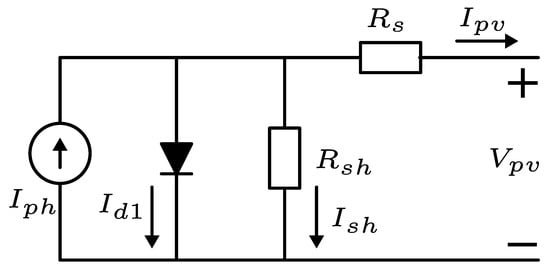
Figure 1. Equivalent circuit of single-diode model.

According to the equivalent circuit in Figure 1 and by applying Kirchhoff’s law, the output current of the cell $I_{pv}$ is written as follows:

$$I_{pv}=I_{ph}-I_d-I_{sh}$$

(1)

The expression of the current $I_d$ is given as follows:

$$I_d=I_{sd}\left[exp\left({\displaystyle \frac{q(V_{pv}+I_{pv}{R}_s)}{nkT}}\right)-1\right]$$

(2)

where k is the Boltzmann constant, and its value is 1.38064852 × 10⁻²³ J/K; q represents the electric charge, and its value is 1.6021764 × 10⁻¹⁹ C; $I_{sd}$ represents the reverse saturation current of the diode; n is the ideality factor of the diode; T is the cell temperature in Kelvin; $V_{pv}$ is the PV cell output voltage; and $R_s$ is the series resistance.

The following equation is used to compute the current of the shunt resistance $I_{sh}$:

$$I_{sh}={\displaystyle \frac{V_{pv}+I_{pv}{R}_s}{R_{sh}}}$$

(3)

where $R_{sh}$ is the shunt resistance.

Substituting the current expressions (2) and (3) into (1) gives the PV cell output current for SDM as follows [25]:

$$I_{pv}=I_{ph}-I_{sd}\left[exp\left({\displaystyle \frac{q(V_{pv}+I_{pv}{R}_s)}{nkT}}\right)-1\right]-{\displaystyle \frac{V_{pv}+I_{pv}{R}_s}{R_{sh}}}$$

(4)

Therefore, after excluding the known parameters, the SDM has 5 unknown parameters, $X=\left[I_{ph},I_{sd},R_{sh},R_s,n\right]$, that need to be identified.

2.2. Double-Diode Model

The double-diode model (DDM) is similar to the SDM, except in this model, a second diode is added in parallel to the first diode, so it more accurately describes the physical effects of the p–n junction. In this model, the first diode represents the diffusion current in the junction, and the other diode models the recombination effects in the space-charge region.

By applying Kirchhoff’s law to the equivalent circuit of the DDM in Figure 2, the output current of the cell $I_{pv}$ is written as follows:

$$I_{pv}=I_{ph}-I_{d1}-I_{d2}-I_{sh}$$

(5)

Figure 2. Equivalent circuit of double-diode model.

Using the same procedure as for the SDM, Equation (6) is produced [38].

$$\begin{array}{cc}\hfill I_{pv}=I_{ph}& -I_{sd1}\left[exp\left({\displaystyle \frac{q(V_{pv}+I_{pv}{R}_s)}{n_{1}kT}}\right)-1\right]\hfill \\ \hfill & -I_{sd2}\left[exp\left({\displaystyle \frac{q(V_{pv}+I_{pv}{R}_s)}{n_{2}kT}}\right)-1\right]\hfill \\ \hfill & -{\displaystyle \frac{V_{pv}+I_{pv}{R}_s}{R_{sh}}}\hfill \end{array}$$

(6)

where $I_{sd1}$ and $I_{sd2}$ represent the diffusion and saturation currents, respectively, and $n_1$ and $n_2$ are the ideality factors of diffusion and recombination for the diodes, respectively.

Therefore, after excluding the known parameters, the DDM has 7 unknown parameters, $X=\left[I_{ph},I_{sd1},I_{sd2},R_{sh},R_s,n_1,n_2\right]$, that can be estimated.

2.3. Three-Diode Model

The three-diode model (TDM) is shown in Figure 3; in this model, three diodes are considered parallel to the current source. This model is more complex than the SDM and DDM. Moreover, it is more accurate than the previous two models.

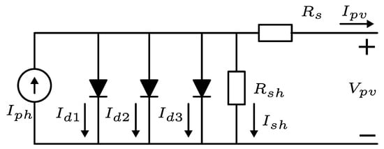
Figure 3. Equivalent circuit of three-diode model.

By applying Kirchhoff’s law to the equivalent circuit of the TDM in Figure 3, the output current of the cell $I_{pv}$ is written as follows [30]:

$$I_{pv}=I_{ph}-I_{d1}-I_{d2}-I_{d3}-I_{sh}$$

(7)

Using the same procedure as for the SDM and DDM, Equation (7) can be rewritten, and Equation (8) is obtained:

$$\begin{array}{cc}\hfill I_{pv}=I_{ph}& -I_{sd1}\left[exp\left({\displaystyle \frac{q(V_{pv}+I_{pv}{R}_s)}{n_{1}kT}}\right)-1\right]\hfill \\ \hfill & -I_{sd2}\left[exp\left({\displaystyle \frac{q(V_{pv}+I_{pv}{R}_s)}{n_{2}kT}}\right)-1\right]\hfill \\ \hfill & -I_{sd3}\left[exp\left({\displaystyle \frac{q(V_{pv}+I_{pv}{R}_s)}{n_{3}kT}}\right)-1\right]\hfill \\ \hfill & -{\displaystyle \frac{V_{pv}+I_{pv}{R}_s}{R_{sh}}}\hfill \end{array}$$

(8)

Therefore, after excluding the known parameters, the TDM has 9 unknown parameters, $X=\left[I_{ph},I_{sd1},I_{sd2},I_{sd3},R_{sh},R_s,n_1,n_2,n_3\right]$, that need to be estimated.

2.4. Photovoltaic Module Model

The single-diode PV module model (PVM) is generally used in the literature; this model consists of several solar cells connected in series and in parallel to generate specific amounts of voltage and current; this model equivalent circuit is shown in Figure 4.

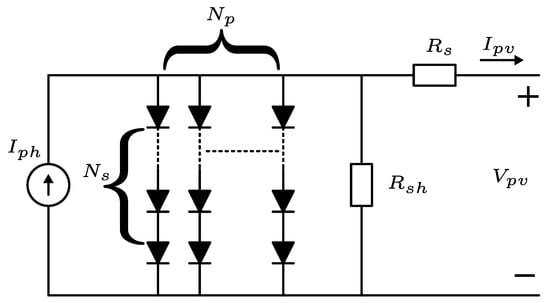
Figure 4. Equivalent circuit of PV module model.

The PV module output current $I_{pv}$ is written as follows [48]:

$$I_{pv}=I_{ph}{N}_p-I_{sd}{N}_p\left[exp\left({\displaystyle \frac{q\left\{V_{pv}+\frac{N_s{I}_{pv}{R}_s}{N_p}\right\}}{nkT{N}_s}}\right)-1\right]-{\displaystyle \frac{V_{pv}+\frac{N_s{I}_{pv}{R}_s}{N_p}}{\frac{N_s{R}_{sh}}{N_p}}}$$

(9)

where $N_p$ and $N_s$ represent the number of cells in parallel and series, respectively. Since the solar cells are typically connected in series, the $N_p$ value equals 1. As a result, the following modification is made to the final PV module output current:

$$I_{pv}=I_{ph}-I_{sd}\left[exp\left({\displaystyle \frac{q(V_{pv}+N_s{I}_{pv}{R}_s)}{nkT{N}_s}}\right)-1\right]-{\displaystyle \frac{V_{pv}+N_s{I}_{pv}{R}_s}{N_s{R}_{sh}}}$$

(10)

3. Objective Function

Table 1 lists the unknown parameters for the PV models based on Equations (4)–(10). Estimating these parameters can be framed as an optimization problem, requiring the definition of an objective function to characterize it.

Table 1. The unknown parameters of the considered PV models.

Parameter	PV Model
	SDM	DDM	TDM	PVM
$I_{ph}$	✓	✓	✓	✓
$I_{sd}$	✓			✓
$I_{sd1}$		✓	✓
$I_{sd2}$		✓	✓
$I_{sd3}$			✓
n	✓			✓
$n_1$		✓	✓
$n_2$		✓	✓
$n_3$			✓
$R_s$	✓	✓	✓	✓
$R_{sh}$	✓	✓	✓	✓

✓: The unknown parameter for each PV model.

The objective is to minimize the error between the actual measured current $I_{mes}$ obtained experimentally and the estimated current $I_{est}$. In the literature, the root-mean-square error (RMSE) is used as the objective function. The formulation of the RMSE is presented in Equation (11).

$$RMSE\left(X\right)=\sqrt{{\displaystyle \frac{1}{N_m}}\sum _1^{N_m}{f}_M{(V_{pv},I_{pv},X)}^2}$$

(11)

where X is the vector of unknown parameters to be estimated, $N_m$ is the number of measured data points, and M represents the type of PV model $M=\left\{\mathrm{SDM},\mathrm{DDM},\mathrm{TDM},\mathrm{and}\mathrm{PVM}\right\}$. $f_M$ is also the error function, which is defined for different PV models as follows:

$$\begin{array}{cc}\hfill f_{SDM}(V_{pv},I_{pv},X)=I_{ph}& -I_{sd}\left[exp\left({\displaystyle \frac{q(V_{pv}+I_{pv}{R}_s)}{nkT}}\right)-1\right]\hfill \\ \hfill & -{\displaystyle \frac{V_{pv}+I_{pv}{R}_s}{R_{sh}}}-I_{pv}\hfill \end{array}$$

(12)

$$\begin{array}{cc}\hfill f_{DDM}(V_{pv},I_{pv},X)=I_{ph}& -I_{sd1}\left[exp\left({\displaystyle \frac{q(V_{pv}+I_{pv}{R}_s)}{n_{1}kT}}\right)-1\right]\hfill \\ \hfill & -I_{sd2}\left[exp\left({\displaystyle \frac{q(V_{pv}+I_{pv}{R}_s)}{n_{2}kT}}\right)-1\right]\hfill \\ \hfill & -{\displaystyle \frac{V_{pv}+I_{pv}{R}_s}{R_{sh}}}-I_{pv}\hfill \end{array}$$

(13)

$$\begin{array}{cc}\hfill f_{TDM}(V_{pv},I_{pv},X)=I_{ph}& -I_{sd1}\left[exp\left({\displaystyle \frac{q(V_{pv}+I_{pv}{R}_s)}{n_{1}kT}}\right)-1\right]\hfill \\ \hfill & -I_{sd2}\left[exp\left({\displaystyle \frac{q(V_{pv}+I_{pv}{R}_s)}{n_{2}kT}}\right)-1\right]\hfill \\ \hfill & -I_{sd3}\left[exp\left({\displaystyle \frac{q(V_{pv}+I_{pv}{R}_s)}{n_{3}kT}}\right)-1\right]\hfill \\ \hfill & -{\displaystyle \frac{V_{pv}+I_{pv}{R}_s}{R_{sh}}}-I_{pv}\hfill \end{array}$$

(14)

$$\begin{array}{cc}\hfill f_{PVM}(V_{pv},I_{pv},X)=I_{ph}& -I_{sd}\left[exp\left({\displaystyle \frac{q(V_{pv}+N_s{I}_{pv}{R}_s)}{nkT{N}_s}}\right)-1\right]\hfill \\ & -{\displaystyle \frac{V_{pv}+N_s{I}_{pv}{R}_s}{N_s{R}_{sh}}}-I_{pv}\hfill \end{array}$$

(15)

Two approaches are used in this paper to obtain two distinct objective functions:

• In the first approach, the objective function is $Ob{j}_1=RMSE\left(X\right)$, and the $I_{est}$ used to calculate the RMSE is based on $I_{mes}$ and the measured voltage $V_{mes}$ values, as shown in Figure 5, which gives the following approximation:

  $$I_{est}-I_{mes}\approx f_M(V_{mes},I_{mes},X)$$

  (16)
  

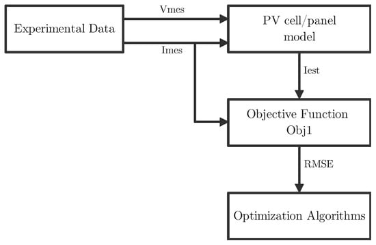  Figure 5. Concept of objective function $Ob{j}_1$ calculation.
• For the second approach, the objective function is $Ob{j}_2$, and the estimated current $I_{est}$ is obtained by using the Newton–Raphson method to solve nonlinear Equations (12)–(15) for a given voltage value ($V_{mes}$), as shown in Figure 6. Moreover, according to this, the objective function is defined as follows:

  $$Ob{j}_2=\sqrt{{\displaystyle \frac{1}{N_m}}\sum _1^{N_m}{(I_{est}-I_{mes})}^2}$$

  (17)

  where $I_{est}$ in (17) is found using the Newton–Raphson method.
  

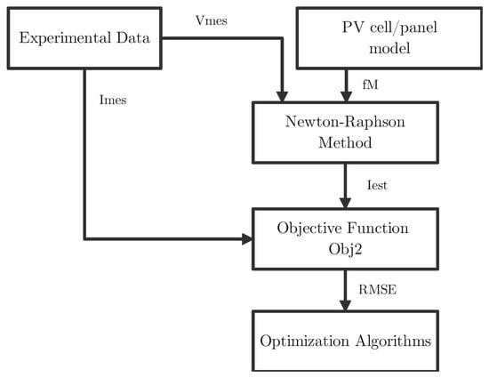  Figure 6. Concept of objective function $Ob{j}_2$ calculation.

The advantage of using the Newton–Raphson method to formulate the objective function $Ob{j}_2$ is to minimize the RMSE to more possible values, compared to the value obtained by most of the algorithms in the literature (in the range from 9.86 × 10⁻⁴ to 1 × 10⁻³).

Meanwhile, to evaluate the performance of the algorithm more accurately, the relative error ($R_e$) is used to express the error value between the simulated and actual data at each measurement point, and the equation is shown in (18). This formula is used to derive a criterion known as the current relative error, which is used to assess the accuracy of the estimated parameters [53]:

$$R_e={\displaystyle \frac{I_{mes}-I_{est}}{I_{mes}}}$$

(18)

4. Metaheuristic Algorithms for PV Model Parameter Extraction

Table 2 summarizes previous works on PV model parameter extraction using metaheuristic optimization algorithms. It presents the algorithm, the model type, the objective function used in each reference, and the pros and cons of the employed method.

Table 2. A review of metaheuristic optimization algorithms used for parameter extraction from solar PV models.

Optimization Algorithm	Ref.	SDM	DDM	TDM	PVM	${\mathit{Obj}}_1$	${\mathit{Obj}}_2$	Pros	Cons
Opposition-Based Exponential Distribution Optimizer (OBEDO)	[42]	✓	✓	✓	✓	✓	✗	Efficient and accurate parameter extraction with superior convergence speed.	Its performance may vary across different problem domains.
Multi-Source Guided Teaching–Learning-Based Optimization (MSGTLBO)	[43]	✓	✓	✗	✓	✓	✗	Enhanced accuracy and reliability through multi-source guided strategies.	Relatively slow initial convergence.
Similarity-Guided Differential Evolution (SGDE)	[54]	✓	✓	✗	✓	✓	✗	Simultaneously extracts parameters for multiple PV models, improving accuracy and convergence.	The approach may be complex due to managing multiple subpopulations and task relationships.
Artificial Parameter-Less Optimization algorithm (APLO)	[55]	✓	✓	✗	✓	✓	✗	No need for control parameters, simplifying implementation while maintaining a good exploration–exploitation balance.	Its performance can be further improved, particularly for specific models like the DDM.
Hybrid Grey Wolf Optimizer and Cuckoo Search (GWOCS)	[56]	✓	✓	✗	✓	✓	✗	Balances exploration and exploitation effectively, leading to fast convergence and high solution accuracy.	The hybrid approach may increase computational complexity compared to simpler algorithms.
War Strategy Optimization (WSO)	[35]	✓	✓	✗	✓	✓	✓	Integrates the Newton–Raphson method to improve accuracy in parameter extraction.	Increased computational time complexity due to the use of the Newton–Raphson method.
Modified Salp Swarm optimization (MSSA)	[45]	✓	✓	✗	✓	✓	✗	Improved exploration and reduced premature convergence, leading to better optimal solutions.	The modified approach may require fine-tuning to handle more complex PV models effectively.
Laplace’s Cross-Search mechanism (LCS) and the Nelder–Mead simplex method (NM) (LCNMSE)	[57]	✓	✓	✗	✓	✓	✗	The LCNMSE algorithm enhances parameter extraction accuracy and efficiently balances exploration and exploitation.	It may struggle with complex optimization problems and is sensitive to specific parameter configurations.
Enhanced Social Network Search Algorithm (ESNSA)	[58]	✓	✓	✓	✓	✓	✗	The ESNSA is highly accurate, robust, and fast-convergent, outperforming other methods in extracting parameters for different PV modules.	The ESNSA may require complex parameter tuning and optimization strategies to maintain its efficiency across various models.
Hybrid Adaptive Teaching–Learning-based optimization with Differential Evolution (ATLDE)	[59]	✓	✓	✗	✓	✓	✗	The ATLDE algorithm offers high accuracy, reliability, and efficient use of computing resources, with significant improvements in PV model parameter identification.	The method may require further refinement for real-world applications under varying temperature conditions and more accurate results for the double-diode model.
Delayed Dynamic Step Shuffling Frog-Leaping Algorithm (DDSFLA)	[49]	✓	✓	✗	✓	✓	✗	The DDSFLA improves convergence speed and accuracy, offering strong optimization stability across varying temperatures and light intensities for PV model parameter extraction.	The DDSFLA requires continuous adjustment of multiple parameters, which may complicate its application and expansion.
Weighted mean of vectors (INFO)	[36]	✓	✓	✗	✓	✓	✗	The INFO algorithm provides the highest accuracy and reliability in parameter extraction, closely matching the manufacturer’s datasheet values and outperforming other metaheuristic algorithms in PV modeling.	The study relies on various comparison algorithms, which may complicate selecting the best approach for specific PV systems.
Gradient-Based Optimizer (GBO)	[60]	✓	✓	✓	✗	✓	✗	The GBO algorithm provides highly accurate parameter estimations for PV models, offering superior performance compared to ten other algorithms. It has fast convergence and balanced exploitation.	The GBO’s performance relies heavily on the availability of accurate experimental data, and it may require adaptation for more complex PV models with multiple diodes or varying conditions.
Tree Seed Algorithm (TSA)	[61]	✗	✗	✗	✓	✓	✗	The TSA demonstrated superior performance in estimating parameters for the STM6-40/36 PV module, achieving the lowest RMSE, faster convergence, and greater robustness than other algorithms.	While the TSA outperformed other algorithms in [61], its application may need further improvement or adaptation for more complex PV models or varying conditions.
Enhanced Adaptive Differential Evolution Algorithm (EJADE)	[46]	✓	✓	✗	✓	✓	✗	The EJADE offers fast, accurate, and reliable parameter extraction for various PV models. Its performance is superior in terms of convergence speed and accuracy compared to existing algorithms. It also demonstrates good practicality under different irradiance and temperature conditions.	The EJADE does not address multi-objective optimization problems or conditions like partial shading, which could limit its application in more complex real-world scenarios.
Tree Growth Algorithm (TGA)	[29]	✓	✓	✓	✓	✓	✗	The TGA provides accurate and efficient parameter extraction for solar cells and PV modules, outperforming other optimization algorithms.	The algorithm has not been tested under partial shading conditions, which could limit its application in certain real-world PV system scenarios.
Gaining–Sharing Knowledge (GSK)	[32]	✓	✓	✗	✓	✓	✗	The GSK algorithm offers high accuracy, robustness, and convergence in PV model parameter extraction.	The population size significantly impacts performance, and an optimal value needs to be selected for the best results.
Either–Or Teaching–Learning-Based Algorithm (EOTLBO)	[50]	✓	✓	✗	✓	✓	✗	EOTLBO offers improved convergence speed and accuracy in PV model parameter extraction, outperforming several other algorithms.	The algorithm relies on a chaotic map for selecting learning strategies, which may require further optimization for more efficient parameter adjustments.
Tunicate Swarm Algorithm (TSA)	[33]	✓	✗	✗	✓	✓	✗	The TSA demonstrates high accuracy, reliability, and robustness in estimating the parameters of solar PV models, outperforming other optimization algorithms.	The TSA’s performance is limited to standard temperature conditions, and its applicability may need further testing under varying environmental conditions.
Moth–Flame Optimization (MFO)	[34]	✓	✗	✗	✓	✓	✗	The proposed hybrid methodology, combining numerical methods and MFO, accurately extracts PV model parameters under varying irradiance and temperature conditions, offering robust energy prediction and fault diagnosis capabilities.	The methodology depends on the accuracy of the translation from real-world conditions to standard test conditions, which could introduce errors if the weather data need to be more accurate or consistent.
Comprehensive Learning Jaya Algorithm (CLJAYA)	[48]	✓	✓	✗	✓	✓	✗	The CLJAYA is efficient and straightforward, requiring only essential population size and terminal conditions for optimization. It provides superior performance in parameter extraction from PV models, offering better accuracy and fewer function evaluations than other algorithms.	While the CLJAYA’s performance is effective in many cases, it might still be limited in highly complex or constrained optimization problems where additional control parameters could help guide the search more effectively.
Enhanced Lévy Flight Bat Algorithm (ELBA)	[28]	✓	✓	✗	✓	✓	✗	The ELBA provides highly competitive performance for extracting parameters from PV models, offering superior accuracy, robustness, and convergence speed compared to other metaheuristic algorithms. It also has a relatively short simulation time, making it an efficient solution.	While the ELBA performs well in PV parameter extraction, its application to other complex optimization problems in renewable energy may require further testing to ensure consistent performance across diverse scenarios.
Forensic-Based Investigation Algorithm (FBIA)	[47]	✓	✓	✓	✗	✓	✗	The FBIA effectively extracts the parameters of various PV models (SDM, DDM, TDM) with high accuracy, producing consistent results with minimal error, making it a strong competitor with other optimization techniques.	Despite its success, the FBIA may require further validation across a wider range of PV models and real-world scenarios to confirm its versatility and general applicability in parameter extraction tasks.
Nutcracker Optimizer Algorithm (NOA)	[37]	✓	✓	✓	✓	✓	✗	The NOA excels in parameter extraction for PV models (SDM, DDM, TDM), outperforming traditional algorithms (PSO, WOA) in terms of accuracy and efficiency (execution time). It is well suited for solar cell problems, offering the best performance across multiple models.	While the NOA shows promising results, further testing with diverse materials (e.g., arsenic gallium, perovskite) and conditions must confirm its effectiveness in broader PV applications and various operational environments.
Flood Algorithm (FLA)	This paper	✓	✓	✓	✓	✓	✓	High accuracy; robust and efficient	There is a igher computational cost with $Ob{j}_2$.

✓: used, ✗: not used

This paper utilizes algorithms not previously applied in the literature to estimate PV cell/module parameters, along with those used before. To avoid significantly increasing the paper’s length, brief descriptions of each algorithm are provided in Table 3 rather than offering extensive details.

Table 3. A summary of the metaheuristic algorithms used in this paper.

Optimization Algorithm	Summary
FLA	See the Section 5
INFO	The weIghted meaN oF vectOrs (INFO) algorithm [62] is a population-based algorithm where the population is a set of vectors that demonstrate possible solutions. INFO has three main operators that update the vectors’ positions in each generation (updating rule, vector combining, and local search).
GTO	The Artificial Gorilla Troops Optimizer (GTO) [63] algorithm is inspired by gorilla troops’ social intelligence in nature. In the GTO algorithm, five different operators are used for optimization operations simulated based on gorilla behaviors. Three are for the exploration phase (migration to an unknown place, movement to other gorillas, migration toward a known location), and two operators are used for the exploitation phase (following the silverback, competition for adult females).
MGO	The Mountain Gazelle Optimizer (MGO) [64] is inspired by wild mountain gazelles’ social life and hierarchy. The MGO algorithm performs optimization operations using four main factors in the life of mountain gazelles: bachelor male herds; maternity herds; solitary, territorial males; and migration to search for food.
RUN	RUN is an efficient optimization algorithm [65] that uses a specific slope calculation concept based on the Runge–Kutta method as an effective search engine for global optimization.
ALO	The Ant Lion Optimizer (ALO) [66] is inspired by the hunting mechanism of ant lions in nature. This approach implements five main steps of hunting prey: the random walk of ants, building traps, entrapment of ants in traps, catching prey, and re-building traps.
DA	The Dragonfly Algorithm (DA) [67] is inspired by the static and dynamic swarming behaviors of dragonflies in nature. Two essential phases of optimization steps are designed by modeling the social interaction of dragonflies in navigating, searching for food, and avoiding enemies when swarming dynamically or statistically.
WOA	The Whale Optimization Algorithm (WOA) introduced in [68] is inspired by the social behavior of humpback whales. The WOA was modeled mathematically in three main phases: encircling prey, bubble-net attacking method (the exploitation phase), and the search for prey (the exploration phase).
PSO	Particle Swarm Optimization (PSO), introduced by James Kennedy and Russell Eberhart in 1995 [69], is inspired by the social behavior of birds flocking to find food or fish schooling. PSO involves three key steps: initialization of particles, velocity and position updates, and fitness evaluation to guide particles toward the optimal solution.
GA	The Genetic Algorithm (GA), proposed by John Holland in 1975 [70], is inspired by the process of natural selection. The GA consists of three main steps: selection, crossover, and mutation.

5. Flood Algorithm

5.1. Inspiration

The flooding phenomenon inspires this algorithm; it was introduced in [52]. A flood occurs when water overflows onto land that is usually dry. This phenomenon happens when rivers, lakes, or streams receive more water than they can contain, causing the excess water to spill onto the surrounding areas.

Flooding is common during periods of heavy rain, especially when the soil is already saturated and unable to absorb more water. Additionally, floods can occur when snow rapidly melts due to a sudden temperature rise, and the frozen ground cannot absorb the water, leading to overflow.

5.2. Mathematical Modeling of FLA

The mathematical modeling of the FLA takes into consideration the following points:

• The water moving in the path with the highest slope is modeled as the population of the swarm (water mass) moving to the objective function’s best solution (the highest slope).
• The floods cause disturbances in the water (population), leading to more efficient solutions and significantly increasing exploration speed within the search space.
• The amount of water added to the river due to snowmelt or rain, or the amount lost because of rising temperatures or through holes and ponds along the river, is modeled by replacing the weaker solution with a new one.

This algorithm has two main phases, described as follows:

Phase 1: Flood flow

During this phase, the natural flow of water toward the slope or more optimal points is modeled, along with the impact of the soil impermeability coefficient on the flooding phenomenon. The general motion of particles $S_i$ is expressed as

$$S_i^{new}=S_{best}+rand\times (S_j-S_i)$$

(19)

where $rand$ generates random values between 0 and 1, and $S_j$ is the jth random member of the population. Based on (19), the $S_i$-th particle naturally moves toward the slope, approaching a value close to the best value $S_{best}$.

As the water flow in the river increases, the likelihood of flooding or turbulence in the water also increases. The depletion coefficient or flow of water depends on the iterations of the algorithm, as modeled in the following expression:

$$Pk={\displaystyle \frac{1.2}{Iter}}{\left[\sqrt{Ite{r}_{max}\times Ite{r}^2+1}+{\displaystyle \frac{4\times ln\left(\sqrt{Ite{r}_{max}\times Ite{r}^2+1}+\frac{Ite{r}_{max}}{4}\right)}{Ite{r}_{max}\times Iter}}\right]}^{-{\displaystyle \frac{2}{3}}}$$

(20)

where $Pk$ is the water depletion coefficient, $Ite{r}_{max}$ is the maximum generations of the algorithm, and $Iter$ is the current generation of the algorithm.

However, it turns out that the flood event occurs randomly, determined by a randomly generated probability. During the flood, the movement of the water masses will follow the equation of motion, as shown below:

$$S_i^{new}=S_i+\left({\displaystyle \frac{{\left(Pk\right)}^{randn}}{iter}}\right)\times (rand\times (S_{max}-S_{min})+S_{min})$$

(21)

where $randn$ is a normal distribution between infinite negative to infinite positive; $S_{max}$ and $S_{min}$ are the upper and lower bounds of the search space.

The high permeability of the soil causes a low potential for flooding, water seeping into cavities surrounding the river, or evaporation. This phenomenon is modeled by (22), where the potential for flooding increases with lower values of the cost of the objective function.

$$P{e}_i={\left({\displaystyle \frac{f\left(S_i\right)-f_{min}}{f_{max}-f_{min}}}\right)}^2$$

(22)

where $f_{min}$ and $f_{max}$ represent the best and worst values of the optimization function determined up to the current iteration of the FLA.

From the previous equations, the first phase of the FLA is summarized as follows:

$$S_i^{new}=\left\{\begin{array}{c}{S}_i+\left({\displaystyle \frac{{\left(Pk\right)}^{randn}}{iter}}\right)\times (rand\times (S_{max}-S_{min})+S_{min})\mathrm{if}rand>rand+P{e}_i\hfill \\ S_{best}+rand\times (S_j-S_i)\mathrm{otherwise}\hfill \end{array}\right.$$

(23)

A new position $S_i^{new}$ is now generated for the ith swarm. If this new position offers a better value than the previous one, it will replace the old position.

Phase 2: Increase and decrease in water

In the second phase of the FLA, if the value of $Pt$ expressed in (24) is greater than a randomly generated number between 0 and 1, these new particles are introduced into the population and will replace the worst solutions. The new particles will be around the best solution, as shown in (25).

$$Pt=\left|sin\left({\displaystyle \frac{rand}{Iter}}\right)\right|$$

(24)

$$S_e^{new}=S_{best}+rand\times (rand\times (S_{max}-S_{min})+S_{min})$$

(25)

where $e=1:N_e$, and $N_e$ is the number of water particles that evaporate, which are the weakest members of the population. Conversely, when $N_e$ particles (water) are added, the total number of particles in the population remains constant.

This cycle of two phases will continue until the desired number of iterations is completed or the user achieves an acceptable optimal solution. The flowchart of the FLA is illustrated in Figure 7.

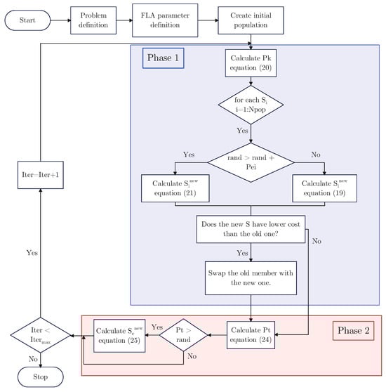
Figure 7. The flowchart of FLA.

6. Results and Discussion

This section applies the FLA to extract the parameters of three PV cell models and one PV module model. The results are compared with the algorithms described in Table 3, with a maximum number of iterations equal to 1000 and a population (particle or agents) size of 50.

The algorithms were evaluated using MATLAB R2021a on a personal computer equipped with an Intel(R) Core(TM) i5-3230M CPU running at 2.60 GHz and 8.00 GB of RAM.

The benchmark data used for the PV cell are from the RTC France silicon cell, while the data for the PV module are from the PhotoWatt PWP-201, as in Table 4 and Appendix A. These are described as follows:

Table 4. Electrical specifications of the PV cell/module.

Cell/Module	Type	Nb of Cells	Temperature [°C]	Irradiance [${\mathbf{W}/\mathbf{m}}^2$]
RTC France cell	Monocrystalline	1	33	1000
Photowatt-PWP 201 PV module	Polycrystalline	36	45	1000

• The RTC France silicon cell is a PV cell with a 57 mm diameter. Its available I–V curve was experimentally obtained under an incident irradiance of 1000 ${\mathrm{W}/\mathrm{m}}^2$ and at an operating temperature of 33 °C, characterized by a set of 26 pairs of current and voltage values [30].
• The Photowatt-PWP 201 PV module is composed of 36 polycrystalline silicon cells connected in series. The experimental data were obtained at an irradiance of 1000 ${\mathrm{W}/\mathrm{m}}^2$ and an operating temperature of 45 °C, characterized by a set of 25 pairs of current and voltage values [48].

In order to ensure that the search space of each problem is the same, the ranges for each parameter are kept the same as those used in the previous literature. Table 5 provides the ranges for each PV cell/module model parameter [30].

Table 5. Parameter ranges of RTC France PV cell and PhotoWatt PWP-201 PV module.

Parameter	Unit	RTC France		PhotoWatt PWP-201
		LB	UB	LB	UB
$I_{ph}$	A	0	1	0	2
$I_{sd}$	$\mathsf{\mu }$A	0	1	0	50
$I_{sd1},I_{sd2},I_{sd3}$	$\mathsf{\mu }$A	0	1	-	-
n	dimensionless	1	2	1	50
$n_1,n_2$	dimensionless	1	2	-	-
$n_3$	dimensionless	2	5	-	-
$R_{sh}$	$\Omega$	0	100	0	1000
$R_s$	$\Omega$	0	0.5	0	2

Notably, the best results for each algorithm applied to extract the parameters of PV models were found and reported after 30 independent runs; these findings were not taken from any other papers.

6.1. SDM for RTC France

Table 6 presents the results of estimating five parameters of the SDM using the FLA and nine other algorithms. To evaluate the precision of the calculated parameters, the RMSE value is used as a metric.

Table 6. Optimal parameters obtained using different algorithms for SDM of RTC France.

Algorithm	Objective Function	${\mathit{I}}_{\mathit{ph}}$ (A)	${\mathit{I}}_{\mathit{sd}}(\mathsf{\mu }$A)	${\mathit{R}}_{\mathit{sh}}\left(\mathbf{\Omega }\right)$	${\mathit{R}}_{\mathit{s}}\left(\mathbf{\Omega }\right)$	n	RMSE
FLA	$Ob{j}_1$	0.76078	0.32302	53.7189	0.036377	1.4812	$9.8602\times {10}^{-4}$
	$Ob{j}_2$	0.76079	0.31069	52.8899	0.036547	1.4773	$7.7299\times {10}^{-4}$
INFO	$Ob{j}_1$	0.76078	0.32302	53.7185	0.036377	1.4812	$9.8602\times {10}^{-4}$
	$Ob{j}_2$	0.76079	0.31069	52.8899	0.036547	1.4773	$7.7299\times {10}^{-4}$
GTO	$Ob{j}_1$	0.76078	0.32302	53.7185	0.036377	1.4812	$9.8602\times {10}^{-4}$
	$Ob{j}_2$	0.76079	0.31069	52.8899	0.036547	1.4773	$7.7299\times {10}^{-4}$
MGO	$Ob{j}_1$	0.76077	0.32616	53.9819	0.036339	1.4822	$9.8619\times {10}^{-4}$
	$Ob{j}_2$	0.76077	0.32853	54.1204	0.036303	1.4829	$7.7788\times {10}^{-4}$
RUN	$Ob{j}_1$	0.76078	0.32483	53.9021	0.036354	1.4817	$9.8621\times {10}^{-4}$
	$Ob{j}_2$	0.76083	0.31916	52.3703	0.036392	1.48	$7.7700\times {10}^{-4}$
ALO	$Ob{j}_1$	0.7612	0.34241	49.5507	0.036041	1.4872	$1.0446\times {10}^{-3}$
	$Ob{j}_2$	0.76061	0.32399	56.3584	0.036416	1.4814	$7.8563\times {10}^{-4}$
DA	$Ob{j}_1$	0.76107	0.42497	55.6897	0.035173	1.5094	$1.1577\times {10}^{-3}$
	$Ob{j}_2$	0.76071	0.25461	51.1086	0.037503	1.4575	$8.4383\times {10}^{-4}$
WOA	$Ob{j}_1$	0.75975	0.33454	74.5599	0.036503	1.4844	$1.2414\times {10}^{-3}$
	$Ob{j}_2$	0.76057	0.24817	50.9716	0.037538	1.455	$8.6332\times {10}^{-4}$
PSO	$Ob{j}_1$	0.76077	0.32651	54.0163	0.036334	1.4823	$9.8623\times {10}^{-4}$
	$Ob{j}_2$	0.76076	0.32553	54.001	0.036344	1.482	$7.7641\times {10}^{-4}$
GA	$Ob{j}_1$	0.75431	0.53119	52.5633	0.02824	1.5342	$1.0253\times {10}^{-2}$
	$Ob{j}_2$	0.75875	0.16744	57.9481	0.038916	1.4175	$1.7810\times {10}^{-3}$

Based on the RMSE results in Table 6, the FLA, similar to the INFO and GTO methods, achieved the lowest RMSE values for both $Ob{j}_1$ and $Ob{j}_2$. However, for $Ob{j}_2$, the RMSE values were significantly lower than for $Ob{j}_1$. In contrast, the GA yielded the highest RMSE values in both cases. The other algorithms also demonstrated lower RMSE values when applied to $Ob{j}_2$ compared to $Ob{j}_1$. For instance, ALO yielded an RMSE of $1.0446\times {10}^{-3}$ for $Ob{j}_1$ and an even lower value of $7.8563\times {10}^{-4}$ for $Ob{j}_2$.

Table 7 presents a statistical comparison of RMSE values for the SDM obtained by different algorithms, evaluated over 30 runs. The key metrics include the best, mean, worst, and standard deviation (std) RMSE values for two objective functions, $Ob{j}_1$ and $Ob{j}_2$.

Table 7. Statistical comparison of RMSE values for the SDM of RTC France obtained from different algorithms after 30 runs.

Algorithm	Objective Function	Best	Mean	Worst	Std
FLA	$Ob{j}_1$	$9.8602\times {10}^{-4}$	$1.0933\times {10}^{-3}$	$1.4385\times {10}^{-3}$	$1.9376\times {10}^{-4}$
	$Ob{j}_2$	$7.7299\times {10}^{-4}$	$9.1403\times {10}^{-4}$	$2.0832\times {10}^{-3}$	$3.5711\times {10}^{-4}$
INFO	$Ob{j}_1$	$9.8602\times {10}^{-4}$	$9.8602\times {10}^{-4}$	$9.8602\times {10}^{-4}$	$1.0451\times {10}^{-16}$
	$Ob{j}_2$	$7.7299\times {10}^{-4}$	$7.7299\times {10}^{-4}$	$7.7299\times {10}^{-4}$	$4.0922\times {10}^{-17}$
GTO	$Ob{j}_1$	$9.8602\times {10}^{-4}$	$9.8602\times {10}^{-4}$	$9.8602\times {10}^{-4}$	$1.7970\times {10}^{-15}$
	$Ob{j}_2$	$7.7299\times {10}^{-4}$	$7.7299\times {10}^{-4}$	$7.7299\times {10}^{-4}$	$1.4634\times {10}^{-16}$
MGO	$Ob{j}_1$	$9.8619\times {10}^{-4}$	$1.4062\times {10}^{-3}$	$2.6109\times {10}^{-3}$	$3.3112\times {10}^{-4}$
	$Ob{j}_2$	$7.7788\times {10}^{-4}$	$1.1025\times {10}^{-3}$	$2.1951\times {10}^{-3}$	$4.1628\times {10}^{-4}$
RUN	$Ob{j}_1$	$9.8621\times {10}^{-4}$	$1.3972\times {10}^{-3}$	$2.2969\times {10}^{-3}$	$3.7991\times {10}^{-4}$
	$Ob{j}_2$	$7.7700\times {10}^{-4}$	$1.1185\times {10}^{-3}$	$1.8515\times {10}^{-3}$	$3.2996\times {10}^{-4}$
ALO	$Ob{j}_1$	$1.0446\times {10}^{-3}$	$2.5586\times {10}^{-3}$	$5.1560\times {10}^{-3}$	$1.2186\times {10}^{-3}$
	$Ob{j}_2$	$7.8563\times {10}^{-4}$	$2.0364\times {10}^{-3}$	$4.4793\times {10}^{-3}$	$8.0598\times {10}^{-4}$
DA	$Ob{j}_1$	$1.1577\times {10}^{-3}$	$4.7057\times {10}^{-3}$	$2.5945\times {10}^{-2}$	$4.5802\times {10}^{-3}$
	$Ob{j}_2$	$8.4383\times {10}^{-4}$	$2.8074\times {10}^{-3}$	$6.8561\times {10}^{-3}$	$1.5218\times {10}^{-3}$
WOA	$Ob{j}_1$	$1.2414\times {10}^{-3}$	$6.6179\times {10}^{-3}$	$4.6018\times {10}^{-2}$	$1.0346\times {10}^{-2}$
	$Ob{j}_2$	$8.6332\times {10}^{-4}$	$6.9254\times {10}^{-3}$	$4.5207\times {10}^{-2}$	$8.6332\times {10}^{-3}$
PSO	$Ob{j}_1$	$9.8623\times {10}^{-4}$	$1.2051\times {10}^{-3}$	$1.5355\times {10}^{-3}$	$1.4963\times {10}^{-4}$
	$Ob{j}_2$	$7.7641\times {10}^{-4}$	$8.8003\times {10}^{-4}$	$1.0929\times {10}^{-3}$	$9.0525\times {10}^{-5}$
GA	$Ob{j}_1$	$1.0253\times {10}^{-2}$	$1.0118\times {10}^{-1}$	$2.7176\times {10}^{-1}$	$6.4085\times {10}^{-2}$
	$Ob{j}_2$	$1.7810\times {10}^{-3}$	$3.4639\times {10}^{-2}$	$1.2259\times {10}^{-1}$	$3.0320\times {10}^{-2}$

Based on Table 7, the FLA demonstrates strong performance in both objective functions, achieving relatively low RMSE values across 30 runs, comparable to other top-performing algorithms like INFO and GTO. For $Ob{j}_1$, the FLA’s best RMSE is $9.8602\times {10}^{-4}$, and its mean RMSE is $1.0933\times {10}^{-3}$, consistently performing well with moderate variability between runs. Similarly, for $Ob{j}_2$, the FLA achieves a best RMSE of $7.7299\times {10}^{-4}$ and a mean of $9.1403\times {10}^{-4}$, indicating reliable results. While the worst-case RMSE values for the FLA show some variability (especially for $Ob{j}_2$, with $2.0832\times {10}^{-3}$), its standard deviation remains moderate, signaling fairly stable performance across different runs.

Compared to other algorithms, the FLA stands out as one of the better-performing methods, but with slightly more variability than INFO and GTO, which consistently produce identical best, mean, and worst RMSE values, indicating perfect stability and precision. In contrast, algorithms like MGO, RUN, ALO, and WOA exhibit higher variability, with much larger standard deviations and worse worst-case RMSE values, particularly for $Ob{j}_2$. The GA performs the worst, with significantly higher RMSE values and extreme variability, making it less reliable. Overall, the FLA strikes a good balance between accuracy and consistency, although it is not quite as stable as the top-performing algorithms like INFO and GTO.

The convergence curve is an additional factor used to compare the performance of the applied algorithms. Figure 8 and Figure 9 present the convergence curves for $Ob{j}_1$ and $Ob{j}_2$, respectively.

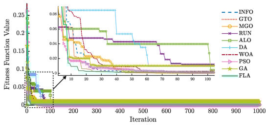
Figure 8. RMSE evolution of different algorithms for the SDM using $Ob{j}_1$.

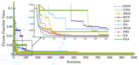
Figure 9. RMSE evolution of different algorithms for the SDM using $Ob{j}_2$.

Based on Figure 8, $Ob{j}_1$ reaches the lowest RMSE value using the FLA after approximately 20 iterations, whereas the other algorithms require more iterations to achieve the same result. Similarly, in Figure 9, the FLA applied to $Ob{j}_2$ reaches the lowest RMSE after about 30 iterations. As in the first case, the other algorithms require more iterations to reach the lowest RMSE.

The average CPU time required to evaluate each algorithm for $Ob{j}_1$ and $Ob{j}_2$ is shown in Figure 10 on a logarithmic scale. Focusing on the FLA, $Ob{j}_1$ has a moderate performance with a CPU time of around 4.2571 s. However, for $Ob{j}_2$, the FLA’s CPU time increases significantly, reaching close to 11.6422 s, indicating that $Ob{j}_2$ is much more computationally expensive for the FLA. Compared to other algorithms like MGO or RUN, which also exhibit long CPU times for $Ob{j}_2$, the FLA’s performance is still relatively moderate but clearly shows a noticeable difference between $Ob{j}_1$ and $Ob{j}_2$ in terms of computational cost.

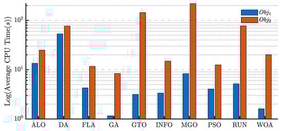
Figure 10. Average CPU times of different algorithms for the SDM using $Ob{j}_1$ and $Ob{j}_2$.

To compare the performance of the FLA for both $Ob{j}_1$ and $Ob{j}_2$ in terms of convergence speed, Figure 11 shows the RMSE evolution of the FLA for the SDM using $Ob{j}_1$ and $Ob{j}_2$. The results indicate that $Ob{j}_2$ requires fewer iterations (around 30 iterations) to reach convergence than $Ob{j}_1$ (around 40 iterations).

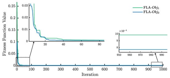
Figure 11. RMSE evolution of the FLA for the SDM using $Ob{j}_1$ and $Ob{j}_2$.

6.2. DDM for RTC France

Table 8 presents a comparative analysis of the two objective functions used to determine the seven optimal parameters for the DDM across different algorithms.

Table 8. Optimal parameters obtained using different algorithms for DDM of RTC France.

Algorithm	Objective Function	${\mathit{I}}_{\mathit{ph}}$ (A)	${\mathit{I}}_{\mathit{sd}1}(\mathsf{\mu }$A)	${\mathit{I}}_{\mathit{sd}2}(\mathsf{\mu }$A)	${\mathit{R}}_{\mathit{sh}}\left(\mathbf{\Omega }\right)$	${\mathit{R}}_{\mathit{s}}\left(\mathbf{\Omega }\right)$	${\mathit{n}}_1$	${\mathit{n}}_2$	RMSE
FLA	$Ob{j}_1$	0.76078	0.22635	0.74607	55.477	0.036739	1.4512	2	$9.8248\times {10}^{-4}$
	$Ob{j}_2$	0.76081	0.78252	0.022129	56.3963	0.038039	1.6766	1.2951	$7.4697\times {10}^{-4}$
INFO	$Ob{j}_1$	0.76078	0.2259	0.74962	55.472	0.036741	1.451	2	$9.8249\times {10}^{-4}$
	$Ob{j}_2$	0.76081	0.070936	1	56.2624	0.037752	1.3648	1.7972	$7.4192\times {10}^{-4}$
GTO	$Ob{j}_1$	0.76078	0.76221	0.2246	55.5538	0.036746	2	1.4505	$9.8249\times {10}^{-4}$
	$Ob{j}_2$	0.7608	0.99998	0.057879	56.5967	0.037859	1.7783	1.3512	$7.4206\times {10}^{-4}$
MGO	$Ob{j}_1$	0.76079	0.16554	0.99999	56.2058	0.037033	1.4262	1.9357	$9.8539\times {10}^{-4}$
	$Ob{j}_2$	0.76081	0.89428	0.059374	55.815	0.03782	1.759	1.3541	$7.4386\times {10}^{-4}$
RUN	$Ob{j}_1$	0.76072	0.61037	0.24035	56.2291	0.036638	1.9808	1.4565	$9.8368\times {10}^{-4}$
	$Ob{j}_2$	0.7608	0.73951	0.095346	55.2112	0.037372	1.7652	1.3886	$7.4753\times {10}^{-4}$
ALO	$Ob{j}_1$	0.76067	0.048667	0.33265	56.6167	0.036205	1.9621	1.4845	$9.9292\times {10}^{-4}$
	$Ob{j}_2$	0.75961	0.45599	0.20574	96.0666	0.035647	1.7011	1.4595	$1.2333\times {10}^{-3}$
DA	$Ob{j}_1$	0.76117	0.22617	1	55.2797	0.035646	1.4564	1.9319	$1.1973\times {10}^{-3}$
	$Ob{j}_2$	0.76056	0.20936	0.3157	59.517	0.035329	1.7816	1.4845	$9.3434\times {10}^{-4}$
WOA	$Ob{j}_1$	0.7608	0.99637	0.33688	63.402	0.034402	1.9998	1.4927	$1.5175\times {10}^{-3}$
	$Ob{j}_2$	0.76035	0.27652	0	56.6761	0.037198	1.4656	1.1476	$8.5821\times {10}^{-4}$
PSO	$Ob{j}_1$	0.76075	0.44127	0.25067	55.623	0.036538	1.9283	1.4605	$9.8446\times {10}^{-4}$
	$Ob{j}_2$	0.76079	0.51674	0.21769	54.3103	0.036863	1.9111	1.4482	$7.5718\times {10}^{-4}$
GA	$Ob{j}_1$	0.759	0.028984	0.61614	88.8715	0.034608	1.4232	1.5697	$2.7955\times {10}^{-3}$
	$Ob{j}_2$	0.75457	0.15308	0.00073012	55.5764	0.037486	1.4108	1.3651	$4.5994\times {10}^{-3}$

For $Ob{j}_1$, the lowest RMSE value was found by the FLA, with a value of $9.8248\times {10}^{-4}$, while the worst values were obtained by the GA, WOA, and DA, respectively. On the other hand, the remaining algorithms produced RMSE values that were very close to those of the FLA. In contrast, for $Ob{j}_2$, the lowest RMSE values were found in the following order: INFO, GTO, MGO, and FLA. However, the GA resulted in the greatest RMSE. Additionally, the parameters obtained by the WOA resulted in a value of 0 for $I_{sd2}$, effectively eliminating the second diode in the model, which means that the WOA failed to find the optimal parameters for the DDM and reduced it to the SDM.

Table 9 presents a statistical comparison of the RMSE values for the DDM case. This table highlights the performance of various algorithms by providing a detailed breakdown of key statistical measures achieved across 30 independent runs.

Table 9. Statistical comparison of RMSE values for the DDM of RTC France obtained from different algorithms after 30 runs.

Algorithm	Objective Function	Best	Mean	Worst	Std
FLA	$Ob{j}_1$	$9.8248\times {10}^{-4}$	$1.3092\times {10}^{-3}$	$3.1263\times {10}^{-3}$	$6.0582\times {10}^{-4}$
	$Ob{j}_2$	$7.4697\times {10}^{-4}$	$9.2550\times {10}^{-4}$	$2.0832\times {10}^{-3}$	$3.4640\times {10}^{-4}$
INFO	$Ob{j}_1$	$9.8249\times {10}^{-4}$	$9.8583\times {10}^{-4}$	$1.0106\times {10}^{-3}$	$5.2189\times {10}^{-6}$
	$Ob{j}_2$	$7.4192\times {10}^{-4}$	$7.6658\times {10}^{-4}$	$1.1914\times {10}^{-3}$	$8.0523\times {10}^{-5}$
GTO	$Ob{j}_1$	$9.8249\times {10}^{-4}$	$9.8542\times {10}^{-4}$	$9.9356\times {10}^{-4}$	$2.1352\times {10}^{-6}$
	$Ob{j}_2$	$7.4206\times {10}^{-4}$	$7.6068\times {10}^{-4}$	$9.6150\times {10}^{-4}$	$3.9294\times {10}^{-5}$
MGO	$Ob{j}_1$	$9.8539\times {10}^{-4}$	$1.3079\times {10}^{-3}$	$1.8035\times {10}^{-3}$	$2.4683\times {10}^{-4}$
	$Ob{j}_2$	$7.4386\times {10}^{-4}$	$9.4012\times {10}^{-4}$	$1.6833\times {10}^{-3}$	$1.8652\times {10}^{-4}$
RUN	$Ob{j}_1$	$9.8368\times {10}^{-4}$	$1.3294\times {10}^{-3}$	$2.6157\times {10}^{-3}$	$4.3623\times {10}^{-4}$
	$Ob{j}_2$	$7.4753\times {10}^{-4}$	$9.0802\times {10}^{-4}$	$1.4786\times {10}^{-3}$	$1.9922\times {10}^{-4}$
ALO	$Ob{j}_1$	$9.9292\times {10}^{-4}$	$2.8439\times {10}^{-3}$	$5.4233\times {10}^{-3}$	$1.1317\times {10}^{-3}$
	$Ob{j}_2$	$1.2333\times {10}^{-3}$	$2.6364\times {10}^{-3}$	$5.3092\times {10}^{-3}$	$1.0332\times {10}^{-3}$
DA	$Ob{j}_1$	$1.1973\times {10}^{-3}$	$5.4322\times {10}^{-3}$	$2.0352\times {10}^{-2}$	$4.6415\times {10}^{-3}$
	$Ob{j}_2$	$9.3434\times {10}^{-4}$	$4.3200\times {10}^{-3}$	$1.1134\times {10}^{-2}$	$2.8024\times {10}^{-3}$
WOA	$Ob{j}_1$	$1.5175\times {10}^{-3}$	$1.7773\times {10}^{-2}$	$4.9250\times {10}^{-2}$	$1.7870\times {10}^{-2}$
	$Ob{j}_2$	$8.5821\times {10}^{-4}$	$8.5519\times {10}^{-3}$	$4.7971\times {10}^{-2}$	$1.1354\times {10}^{-2}$
PSO	$Ob{j}_1$	$9.8446\times {10}^{-4}$	$1.3311\times {10}^{-3}$	$2.0080\times {10}^{-3}$	$2.7563\times {10}^{-4}$
	$Ob{j}_2$	$7.5718\times {10}^{-4}$	$9.3423\times {10}^{-4}$	$1.3519\times {10}^{-3}$	$1.4872\times {10}^{-4}$
GA	$Ob{j}_1$	$2.7955\times {10}^{-3}$	$6.5626\times {10}^{-2}$	$1.8567\times {10}^{-1}$	$5.5880\times {10}^{-2}$
	$Ob{j}_2$	$4.5994\times {10}^{-3}$	$2.1612\times {10}^{-2}$	$7.5854\times {10}^{-2}$	$1.7390\times {10}^{-2}$

In the DDM scenario, the FLA shows reasonable performance, with some variability between runs. For $Ob{j}_1$, the FLA achieves the best RMSE of $9.8248\times {10}^{-4}$, but the mean RMSE rises to $1.3092\times {10}^{-3}$, and the worst RMSE reaches $3.1263\times {10}^{-3}$, indicating a noticeable spread across runs. For $Ob{j}_2$, the FLA performs slightly better, with the best RMSE of $7.4697\times {10}^{-4}$ and a mean of $9.2550\times {10}^{-4}$, although the worst case reaches $2.0832\times {10}^{-3}$. The standard deviations, particularly $6.0582\times {10}^{-4}$ for $Ob{j}_1$ and $3.4640\times {10}^{-4}$ for $Ob{j}_2$, suggest moderate variation, making the FLA fairly reliable but less stable than other leading algorithms.

Compared to other algorithms, the FLA’s performance is decent but outshone by INFO and GTO, demonstrating near-perfect stability with minimal standard deviations and consistently low RMSE values. INFO and GTO have much smaller spreads between their best, mean, and worst RMSE, indicating superior stability and precision. Algorithms like MGO, RUN, and PSO also perform better than the FLA, though they show more variation in their results than INFO and GTO. On the other hand, algorithms like the ALO, DA, and WOA perform significantly worse, with much higher RMSE values and extreme variability. Again, the GA shows the poorest performance, with very high mean RMSE values and substantial fluctuations, highlighting its unreliability in this case.

Figure 12 and Figure 13 illustrate the convergence curves of ten algorithms for the DDM on the RTC France cell using $Ob{j}_1$ and $Ob{j}_2$, respectively.

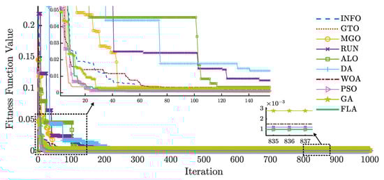
Figure 12. RMSE evolution of different algorithms for the DDM using $Ob{j}_1$.

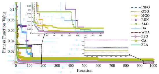
Figure 13. RMSE evolution of different algorithms for the DDM using $Ob{j}_2$.

The lowest RMSE value using the FLA is achieved after 30 iterations for $Ob{j}_1$ and 580 iterations for $Ob{j}_2$. In contrast, for $Ob{j}_1$, PSO and GTO reach their lowest RMSE values at approximately iterations 24 and 28, respectively, while other algorithms require more iterations than the FLA. For $Ob{j}_2$, the FLA requires more iterations to reach the lowest RMSE.

Figure 14 shows the average CPU time for each algorithm applied to $Ob{j}_1$ and $Ob{j}_2$ in the DDM case. For $Ob{j}_1$, the FLA achieves the lowest CPU time compared to $Ob{j}_2$. For $Ob{j}_2$, FLA also demonstrates significantly lower CPU time than most other algorithms, including the ALO, DA, MGO, and RUN, and remains among the fastest overall, along with the GA. In contrast, for $Ob{j}_1$, algorithms such as the ALO, DA, GTO, INFO, MGO, RUN, and WOA exhibit notably higher CPU times, with GTO and MGO being particularly time-intensive. Overall, the FLA is the most efficient choice for minimizing CPU time for both objectives.

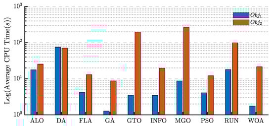
Figure 14. Average CPU times of different algorithms for the DDM using $Ob{j}_1$ and $Ob{j}_2$.

Figure 15 shows the convergence curves of the FLA for the two formulated objective functions. The curve for $Ob{j}_1$ converges at iteration 30, reaching a lower fitness value than $Ob{j}_2$. However, by iteration 580, $Ob{j}_2$ converges to a much lower value than $Ob{j}_1$.

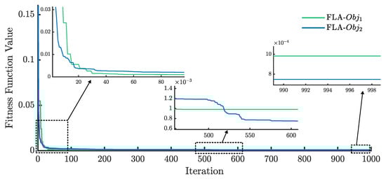
Figure 15. RMSE evolution of the FLA for the DDM using $Ob{j}_1$ and $Ob{j}_2$.

6.3. TDM for RTC France

Table 10 presents the results of estimating the nine parameters of the TDM using the FLA and nine other algorithms. Similar to the previous cases, the RMSE value was used as a metric to evaluate the precision of the estimated parameters.

Table 10. Optimal parameters obtained using different algorithms for TDM of RTC France.

Algorithm	Objective Function	${\mathit{I}}_{\mathit{ph}}$ (A)	${\mathit{I}}_{\mathit{sd}1}(\mathsf{\mu }$A)	${\mathit{I}}_{\mathit{sd}2}(\mathsf{\mu }$A)	${\mathit{I}}_{\mathit{sd}3}(\mathsf{\mu }$A)	${\mathit{R}}_{\mathit{sh}}\left(\mathbf{\Omega }\right)$	${\mathit{R}}_{\mathit{s}}\left(\mathbf{\Omega }\right)$	${\mathit{n}}_1$	${\mathit{n}}_2$	${\mathit{n}}_3$	RMSE
FLA	$Ob{j}_1$	0.76078	0.37926	0.23913	1	55.752	0.036736	1.9999	1.4551	2.3982	$9.8034\times {10}^{-4}$
	$Ob{j}_2$	0.7608	0.12404	0.99944	0.99988	55.7053	0.037417	1.4039	1.8775	2	$7.3652\times {10}^{-4}$
INFO	$Ob{j}_1$	0.76078	0.23981	0.50536	0.99651	55.7903	0.036704	1.4556	2	2.628	$9.8057\times {10}^{-4}$
	$Ob{j}_2$	0.76081	0.058383	0.99995	1	56.4072	0.037863	1.3517	1.7794	2	$7.3488\times {10}^{-4}$
GTO	$Ob{j}_1$	0.76078	0.25444	0.26388	0.94525	55.4506	0.036668	1.4603	2	2.3906	$9.8053\times {10}^{-4}$
	$Ob{j}_2$	0.76081	0.14143	0.99992	0.64361	54.9686	0.037398	1.413	1.9131	2.0011	$7.4035\times {10}^{-4}$
MGO	$Ob{j}_1$	0.76077	4.0809 × 10−10	0.30324	0.16801	54.2268	0.036427	1.1065	1.4758	2.0247	$9.8475\times {10}^{-4}$
	$Ob{j}_2$	0.76083	0.040845	0.99664	0.99987	56.0589	0.038183	1.3273	1.7568	2	$7.3692\times {10}^{-4}$
RUN	$Ob{j}_1$	0.76078	0.26114	0.50826	0.0013801	55.3044	0.036519	1.4635	1.9999	2.5443	$9.8393\times {10}^{-4}$
	$Ob{j}_2$	0.7608	0.12224	0.7248	0.41369	55.0055	0.03727	1.4054	1.8007	2.0487	$7.4631\times {10}^{-4}$
ALO	$Ob{j}_1$	0.76157	0.048748	0.29083	0.047366	44.4477	0.036326	1.6892	1.4734	4.8838	$1.1400\times {10}^{-3}$
	$Ob{j}_2$	0.75953	0.41814	0.05845	0.99564	94.7985	0.035498	1.5078	1.9647	3.5215	$1.2576\times {10}^{-3}$
DA	$Ob{j}_1$	0.76145	0.16847	0.39522	0.79019	55.4341	0.035275	1.4424	1.7035	2.0325	$1.3750\times {10}^{-3}$
	$Ob{j}_2$	0.75985	0.00039197	0.48379	0.50386	87.1031	0.03481	1.4181	1.5231	3.2742	$1.1916\times {10}^{-3}$
WOA	$Ob{j}_1$	0.76053	0.31514	0	0.8076	55.3758	0.036603	1.4787	1.0106	4.99	$1.0186\times {10}^{-3}$
	$Ob{j}_2$	0.76012	0.2675	0.14688	0.16213	70.921	0.035443	1.5212	1.4848	2.0083	$9.6913\times {10}^{-4}$
PSO	$Ob{j}_1$	0.76079	0.44256	0.16469	0.77123	56.0875	0.036948	1.7934	1.4278	2.3131	$9.8410\times {10}^{-4}$
	$Ob{j}_2$	0.76078	0.21378	0.45316	0.50607	54.7183	0.036789	1.4477	1.8585	2.9743	$7.5915\times {10}^{-4}$
GA	$Ob{j}_1$	0.76105	0.64277	0.24022	0.73937	62.0273	0.032876	1.6653	1.502	3.4811	$2.1754\times {10}^{-3}$
	$Ob{j}_2$	0.7617	0	0.30928	0.66406	60.0147	0.032723	1.518	1.4756	2.738	$5.9480\times {10}^{-3}$

Based on Table 10, the FLA achieves the lowest RMSE value of $9.8034\times {10}^{-4}$ for $Ob{j}_1$, followed in order by GTO, INFO, RUN, PSO, MGO, WOA, ALO, DA, and GA. In contrast, for $Ob{j}_2$, the FLA reaches an RMSE value of $7.3652\times {10}^{-4}$, with INFO achieving a slightly lower value of $7.3488\times {10}^{-4}$. The GA, as in previous cases, has the highest RMSE value.

In the TDM scenario, Table 11 presents a statistical comparison of the RMSE values for the DDM case across 30 independent runs. The FLA shows moderate performance with some variability across runs. For $Ob{j}_1$, the FLA’s best RMSE is $9.8034\times {10}^{-4}$, with a mean RMSE of $1.2355\times {10}^{-3}$ and a worst RMSE reaching $3.5963\times {10}^{-3}$, which indicates a considerable spread. For $Ob{j}_2$, the FLA performs slightly better, achieving a best RMSE of $7.3652\times {10}^{-4}$ and a mean of $8.8318\times {10}^{-4}$, although the worst RMSE value is $2.6448\times {10}^{-3}$. The standard deviations, especially $6.4815\times {10}^{-4}$ for $Ob{j}_1$, suggest moderate run-to-run variability, indicating that while the FLA is effective, it lacks stability in some other algorithms.

Table 11. Statistical comparison of RMSE values for the TDM of RTC France obtained from different algorithms after 30 runs.

Algorithm	Objective Function	Best	Mean	Worst	Std
FLA	$Ob{j}_1$	$9.8034\times {10}^{-4}$	$1.2355\times {10}^{-3}$	$3.5963\times {10}^{-3}$	$6.4815\times {10}^{-4}$
	$Ob{j}_2$	$7.3652\times {10}^{-4}$	$8.8318\times {10}^{-4}$	$2.6448\times {10}^{-3}$	$3.7046\times {10}^{-4}$
INFO	$Ob{j}_1$	$9.8057\times {10}^{-4}$	$9.8339\times {10}^{-4}$	$1.0140\times {10}^{-3}$	$6.0141\times {10}^{-6}$
	$Ob{j}_2$	$7.3488\times {10}^{-4}$	$7.4622\times {10}^{-4}$	$7.6553\times {10}^{-4}$	$9.4123\times {10}^{-6}$
GTO	$Ob{j}_1$	$9.8053\times {10}^{-4}$	$9.9607\times {10}^{-4}$	$1.2865\times {10}^{-3}$	$5.5215\times {10}^{-5}$
	$Ob{j}_2$	$7.4035\times {10}^{-4}$	$7.6774\times {10}^{-4}$	$1.1912\times {10}^{-3}$	$8.0680\times {10}^{-5}$
MGO	$Ob{j}_1$	$9.8475\times {10}^{-4}$	$1.3228\times {10}^{-3}$	$2.2316\times {10}^{-3}$	$2.7031\times {10}^{-4}$
	$Ob{j}_2$	$7.3692\times {10}^{-4}$	$8.8519\times {10}^{-4}$	$1.1729\times {10}^{-3}$	$1.1179\times {10}^{-4}$
RUN	$Ob{j}_1$	$9.8393\times {10}^{-4}$	$1.3668\times {10}^{-3}$	$2.4058\times {10}^{-3}$	$3.9583\times {10}^{-4}$
	$Ob{j}_2$	$7.4631\times {10}^{-4}$	$9.4296\times {10}^{-4}$	$1.8007\times {10}^{-3}$	$2.6162\times {10}^{-4}$
ALO	$Ob{j}_1$	$1.1400\times {10}^{-3}$	$5.6592\times {10}^{-3}$	$1.3377\times {10}^{-3}$	$2.8619\times {10}^{-3}$
	$Ob{j}_2$	$1.2576\times {10}^{-3}$	$2.4783\times {10}^{-3}$	$4.4749\times {10}^{-3}$	$7.6060\times {10}^{-4}$
DA	$Ob{j}_1$	$1.3750\times {10}^{-3}$	$7.0364\times {10}^{-3}$	$2.6435\times {10}^{-2}$	$6.9649\times {10}^{-3}$
	$Ob{j}_2$	$1.1916\times {10}^{-3}$	$4.2839\times {10}^{-3}$	$1.2941\times {10}^{-2}$	$2.9447\times {10}^{-3}$
WOA	$Ob{j}_1$	$1.0186\times {10}^{-3}$	$8.2696\times {10}^{-3}$	$4.3833\times {10}^{-2}$	$1.0353\times {10}^{-2}$
	$Ob{j}_2$	$9.6913\times {10}^{-4}$	$4.7817\times {10}^{-3}$	$1.8643\times {10}^{-2}$	$4.1994\times {10}^{-3}$
PSO	$Ob{j}_1$	$9.8410\times {10}^{-4}$	$1.1778\times {10}^{-3}$	$1.7041\times {10}^{-3}$	$2.0436\times {10}^{-4}$
	$Ob{j}_2$	$7.5915\times {10}^{-4}$	$9.0708\times {10}^{-4}$	$1.1185\times {10}^{-3}$	$1.0805\times {10}^{-4}$
GA	$Ob{j}_1$	$2.1754\times {10}^{-3}$	$6.2686\times {10}^{-2}$	$2.6140\times {10}^{-1}$	$5.7323\times {10}^{-2}$
	$Ob{j}_2$	$5.9480\times {10}^{-3}$	$3.1997\times {10}^{-2}$	$9.3573\times {10}^{-2}$	$2.4710\times {10}^{-2}$

In comparison, INFO and GTO outperform other algorithms, delivering very low RMSE values with minimal standard deviations, indicating highly stable and consistent results. The FLA’s performance is decent, though not as stable as INFO or GTO. MGO and RUN also produce fairly low RMSE values but with a higher degree of variability. Conversely, the ALO, DA, and WOA perform significantly worse, with much higher RMSE values and considerable variability, making them less reliable for the TDM. Again, the GA demonstrates the poorest performance with the highest mean and worst-case RMSE values, showing extreme variability and inconsistency. While the FLA remains competitive, it is less stable and precise than INFO and GTO in the TDM scenario.

Figure 16 and Figure 17 illustrate the convergence curves of ten algorithms for the TDM on the RTC France cell using $Ob{j}_1$ and $Ob{j}_2$, respectively. The lowest RMSE value using the FLA is achieved after 52 iterations for $Ob{j}_1$ and 57 for $Ob{j}_2$. In contrast, for $Ob{j}_1$, PSO and MGO reach their lowest RMSE values at approximately 81 and 114 iterations, respectively, while the other algorithms require more iterations than the FLA. For $Ob{j}_2$, the FLA reaches the lowest RMSE in fewer iterations than the other algorithms.

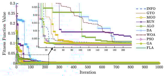
Figure 16. RMSE evolution of different algorithms for the TDM using $Ob{j}_1$.

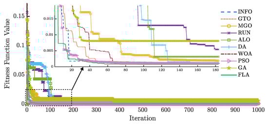
Figure 17. RMSE evolution of different algorithms for the TDM using $Ob{j}_2$.

Figure 18 illustrates the average CPU time for each algorithm applied to $Ob{j}_1$ and $Ob{j}_2$ in the TDM case. The computation time for $Ob{j}_1$ is lower than that for $Ob{j}_2$ across all ten algorithms. The lowest computation time for both objective functions is recorded for the GA. Additionally, the FLA demonstrates significantly lower CPU times than most other algorithms, including the ALO, DA, GTO, INFO, MGO, RUN, and WOA. On the other hand, GTO and MGO exhibit the highest CPU times for $Ob{j}_2$.

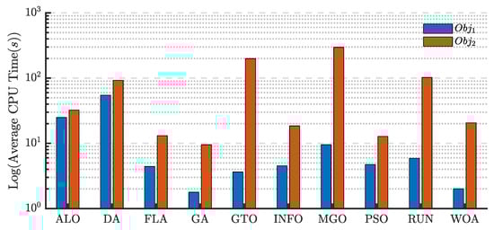
Figure 18. Average CPU times of different algorithms for the TDM using $Ob{j}_1$ and $Ob{j}_2$.

Figure 19 illustrates the convergence curves of the FLA for $Ob{j}_1$ and $Ob{j}_2$. The curve for $Ob{j}_2$ converges at iteration 57, achieving a lower fitness value compared to $Ob{j}_1$, which reaches its lowest RMSE value around iteration 52.

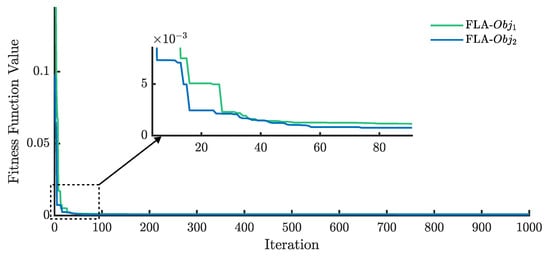
Figure 19. RMSE evolution of the FLA for the TDM using $Ob{j}_1$ and $Ob{j}_2$.

According to the results presented in Table 6, Table 7, Table 8, Table 9, Table 10 and Table 11, the TDM is more accurate than the SDM and DDM in representing the operation of the RTC France cell, as indicated by the lower RMSE values across all applied algorithms, $9.8034\times {10}^{-4}$ for $Ob{j}_1$ and $7.3652\times {10}^{-4}$ for $Ob{j}_2$, using the FLA.

Table 12 and Table 13 presents the estimated current obtained by the FLA using $Ob{j}_1$ and $Ob{j}_2$, respectively, along with the relative error ($R_e$) for the SDM, DDM, and TDM. The consistently low relative error values demonstrate the high accuracy of the estimated parameters.

Table 12. Relative error for each measurement and estimated current values using SDD, DDM, and TDM with FLA ($Ob{j}_1$ is used).

			SDM		DDM		TDM
Data	${\mathit{V}}_{\mathit{mes}}$	${\mathit{I}}_{\mathit{mes}}$	${\mathit{I}}_{\mathit{est}}$	${\mathit{R}}_{\mathit{e}}$	${\mathit{I}}_{\mathit{est}}$	${\mathit{R}}_{\mathit{e}}$	${\mathit{I}}_{\mathit{est}}$	${\mathit{R}}_{\mathit{e}}$
1	−0.2057	0.7640	0.7640876508	−0.0001147262	0.7639839053	0.0000210662	0.7639710499	0.0000378927
2	−0.1291	0.7620	0.7626630443	−0.0008701369	0.7626043792	−0.0007931486	0.7625982263	−0.0007850739
3	−0.0588	0.7605	0.7613552755	−0.0011246227	0.7613377897	−0.0011016301	0.7613376162	−0.0011014020
4	0.0057	0.7605	0.7601539688	0.0004550047	0.7601737059	0.0004290520	0.7601786456	0.0004225567
5	0.0646	0.7600	0.7590551953	0.0012431640	0.7591074466	0.0011744123	0.7591163352	0.0011627167
6	0.1185	0.7590	0.7580423394	0.0012617398	0.7581210623	0.0011580205	0.7581323588	0.0011431371
7	0.1678	0.7570	0.7570916551	−0.0001210767	0.7571881723	−0.0002485764	0.7571999062	−0.0002640769
8	0.2132	0.7570	0.7561413720	0.0011342509	0.7562431396	0.0009998154	0.7562530227	0.0009867598
9	0.2545	0.7555	0.7550868845	0.0005468105	0.7551768875	0.0004276803	0.7551827320	0.0004199443
10	0.2924	0.7540	0.7536638927	0.0004457655	0.7537220865	0.0003685854	0.7537223489	0.0003682375
11	0.3269	0.7505	0.7513909807	−0.0011871829	0.7513991003	−0.0011980018	0.7513935946	−0.0011906657
12	0.3585	0.7465	0.7473538614	−0.0011438197	0.7473016915	−0.0010739337	0.7472918604	−0.0010607642
13	0.3873	0.7385	0.7401172231	−0.0021898756	0.7400111620	−0.0020462587	0.7399999677	−0.0020311005
14	0.4137	0.7280	0.7273822131	0.0008486083	0.7272475880	0.0010335328	0.7272386436	0.0010458191
15	0.4373	0.7065	0.7069726246	−0.0006689661	0.7068508712	−0.0004966330	0.7068469540	−0.0004910885
16	0.4590	0.6755	0.6752801116	0.0003255193	0.6752108654	0.0004280304	0.6752130529	0.0004247920
17	0.4784	0.6320	0.6307582263	0.0019648316	0.6307607384	0.0019608569	0.6307677513	0.0019497604
18	0.4960	0.5730	0.5719283157	0.0018703041	0.5719944116	0.0017549535	0.5720035177	0.0017390615
19	0.5119	0.4990	0.4996069887	−0.0012164103	0.4997056620	−0.0014141524	0.4997138467	−0.0014305545
20	0.5265	0.4130	0.4136487824	−0.0015709017	0.4137332740	−0.0017754818	0.4137383474	−0.0017877662
21	0.5398	0.3165	0.3175101209	−0.0031915354	0.3175460477	−0.0033050481	0.3175472259	−0.0033087709
22	0.5521	0.2120	0.2121549674	−0.0007309786	0.2121231710	−0.0005809954	0.2121211363	−0.0005713980
23	0.5633	0.1035	0.1022513463	0.0120642862	0.1021637256	0.0129108628	0.1021604162	0.0129428379
24	0.5736	−0.0100	−0.0087175199	0.1282480009	−0.0087913668	0.1208633142	−0.0087935316	0.1206468354
25	0.5833	−0.1230	−0.1255074177	−0.0203855099	−0.1255432360	−0.0206767160	−0.1255408253	−0.0206571164
26	0.5900	−0.2100	−0.2084723713	0.0072744223	−0.2083720525	0.0077521308	−0.2083648070	0.0077866331

Table 13. Relative error for each measurement and estimated current values using SDD, DDM, and TDM with FLA ($Ob{j}_2$ is used).

			SDM		DDM		TDM
Data	${\mathit{V}}_{\mathit{mes}}$	${\mathit{I}}_{\mathit{mes}}$	${\mathit{I}}_{\mathit{est}}$	${\mathit{R}}_{\mathit{e}}$	${\mathit{I}}_{\mathit{est}}$	${\mathit{R}}_{\mathit{e}}$	${\mathit{I}}_{\mathit{est}}$	${\mathit{R}}_{\mathit{e}}$
1	−0.2057	0.7640	0.7641494600	−0.0001956087	0.7639406841	0.0000776384	0.7639823499	0.0000231022
2	−0.1291	0.7620	0.7627021479	−0.0009214408	0.7625832870	−0.0007654686	0.7626080692	−0.0007979911
3	−0.0588	0.7605	0.7613737717	−0.0011489365	0.7613372671	−0.0011009429	0.7613464609	−0.0011130321
4	0.0057	0.7605	0.7601545059	0.0004543003	0.7601929827	0.0004037045	0.7601876548	0.0004107102
5	0.0646	0.7600	0.7590390542	0.0012643991	0.7591442512	0.0011259851	0.7591252626	0.0011509702
6	0.1185	0.7590	0.7580107586	0.0013033406	0.7581724526	0.0010903127	0.7581404737	0.0011324456
7	0.1678	0.7570	0.7570457017	−0.0000603838	0.7572488053	−0.0003286728	0.7572048491	−0.0002706065
8	0.2132	0.7570	0.7560848316	0.0012089259	0.7563058489	0.0009169762	0.7562525205	0.0009874232
9	0.2545	0.7555	0.7550223525	0.0006322092	0.7552259706	0.0003627126	0.7551692371	0.0004378065
10	0.2924	0.7540	0.7535973564	0.0005339911	0.7537373805	0.0003483016	0.7536882349	0.0004134815
11	0.3269	0.7505	0.7513272542	−0.0011022888	0.7513558820	−0.0011404157	0.7513290384	−0.0011046481
12	0.3585	0.7465	0.7473053274	−0.0010788186	0.7471905501	−0.0009250503	0.7472017962	−0.0009401155
13	0.3873	0.7385	0.7400846191	−0.0021457341	0.7398355784	−0.0018085016	0.7398899806	−0.0018821674
14	0.4137	0.7280	0.7274261525	0.0007882541	0.7271084803	0.0012246149	0.7272014396	0.0010969236
15	0.4373	0.7065	0.7070258823	−0.0007443359	0.7067504063	−0.0003544321	0.7068416972	−0.0004836478
16	0.4590	0.6755	0.6754002667	0.0001476651	0.6752763417	0.0003311002	0.6753335425	0.0002464210
17	0.4784	0.6320	0.6309981332	0.0015852570	0.6310687734	0.0014734597	0.6310726339	0.0014673513
18	0.4960	0.5730	0.5721746912	0.0014403497	0.5723928448	0.0010596076	0.5723418984	0.0011485192
19	0.5119	0.4990	0.4995389456	−0.0010800450	0.4997908192	−0.0015848080	0.4997026393	−0.0014080948
20	0.5265	0.4130	0.4134848122	−0.0011738974	0.4136498220	−0.0015734190	0.4135827202	−0.0014109449
21	0.5398	0.3165	0.3171614678	−0.0020899986	0.3171678448	−0.0021100943	0.3171480045	−0.0020474078
22	0.5521	0.2120	0.2120165159	−0.0000780114	0.2118652142	0.0006357820	0.2119124913	0.0004127768
23	0.5633	0.1035	0.1026365450	0.0083423395	0.1024015923	0.0106126346	0.1025000979	0.0096608888
24	0.5736	−0.0100	−0.0092986919	0.0701325271	−0.0094965625	0.0503437475	−0.0094374012	0.0562598755
25	0.5833	−0.1230	−0.1243615970	−0.0110698495	−0.1243711751	−0.0111477656	−0.1243299468	−0.0108125759
26	0.5900	−0.2100	−0.2091023162	0.0042746528	−0.2088710364	0.0053760170	−0.2089628171	0.0049389661

Figure 20 illustrates the current–voltage (I-V) characteristics of the RTC France cell based on the SDM, DDM, and TDM, respectively, using the FLA for both $Ob{j}_1$ and $Ob{j}_2$. Similarly, Figure 21 shows the power–voltage (P-V) characteristics of the RTC France cell for the same models and objective functions. The curves demonstrate an excellent match between the observed and simulated data; however, the curves based on $Ob{j}_2$ are more accurate for the SDM, DDM, and TDM. Additionally, the curves derived from the TDM are very close to the experimental data.

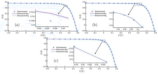
Figure 20. The I-V curves of the FLA for the (a) SDM, (b) DDM, and (c) TDM of RTC France, using $Ob{j}_1$ and $Ob{j}_2$.

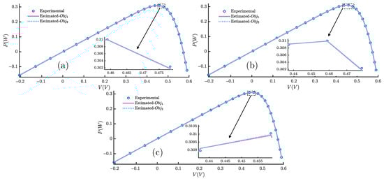
Figure 21. The P-V curves of the FLA for the (a) SDM, (b) DDM, and (c) TDM of RTC France, using $Ob{j}_1$ and $Ob{j}_2$.

6.4. PVM for Photowatt-PWP201

Table 14 presents the results of estimating five parameters of the PVM using ten different algorithms. As in the previous cases, the RMSE value is used as the evaluation metric.

Table 14. Optimal parameters obtained using different algorithms for PVM for Photowatt-PWP201.

Algorithm	Objective Function	${\mathit{I}}_{\mathit{ph}}$ (A)	${\mathit{I}}_{\mathit{sd}}(\mathsf{\mu }$A)	${\mathit{R}}_{\mathit{sh}}\left(\mathbf{\Omega }\right)$	${\mathit{R}}_{\mathit{s}}\left(\mathbf{\Omega }\right)$	n	RMSE
FLA	$Ob{j}_1$	1.0306	3.4613	26.9716	0.033383	1.3506	$2.4252\times {10}^{-3}$
	$Ob{j}_2$	1.0314	2.6381	22.8234	0.034323	49.464	$2.0528\times {10}^{-3}$
INFO	$Ob{j}_1$	1.0305	3.4823	27.2773	0.033369	1.3512	$2.4251\times {10}^{-3}$
	$Ob{j}_2$	1.0314	2.638	22.8225	0.034323	49.4638	$2.0528\times {10}^{-3}$
GTO	$Ob{j}_1$	1.0305	3.4823	27.2773	0.033369	1.3512	$2.4251\times {10}^{-3}$
	$Ob{j}_2$	1.0314	2.638	22.8225	0.034323	49.4638	$2.0528\times {10}^{-3}$
MGO	$Ob{j}_1$	1.0302	3.6764	28.9961	0.033212	1.357	$2.4297\times {10}^{-3}$
	$Ob{j}_2$	1.0314	2.632	22.786	0.03433	49.4552	$2.0529\times {10}^{-3}$
RUN	$Ob{j}_1$	1.0304	3.4561	27.637	0.033422	1.3504	$2.4270\times {10}^{-3}$
	$Ob{j}_2$	1.0314	2.6075	22.7428	0.034364	49.4192	$2.0530\times {10}^{-3}$
ALO	$Ob{j}_1$	1.0262	8.2966	373.7053	0.030673	1.4502	$3.4426\times {10}^{-3}$
	$Ob{j}_2$	1.0225	3.062	589.567	0.034563	50	$3.2886\times {10}^{-3}$
DA	$Ob{j}_1$	1.0205	1.8115	339.9075	0.035972	1.2836	$5.3032\times {10}^{-3}$
	$Ob{j}_2$	1.0366	3.0121	16.3951	0.033637	50	$2.6749\times {10}^{-3}$
WOA	$Ob{j}_1$	1.0208	2.2908	996.613	0.035438	1.3067	$4.7411\times {10}^{-3}$
	$Ob{j}_2$	1.0228	2.9959	350.6043	0.03472	49.916	$3.2687\times {10}^{-3}$
PSO	$Ob{j}_1$	1.0255	7.6265	935.157	0.031024	1.4398	$3.2776\times {10}^{-3}$
	$Ob{j}_2$	1.0315	2.6057	22.5966	0.034361	49.4169	$2.0530\times {10}^{-3}$
GA	$Ob{j}_1$	1.0366	24.5745	439.7364	0.022682	1.5906	$3.2632\times {10}^{-2}$
	$Ob{j}_2$	1.0102	0.056088	757.3038	0.042583	37.9962	$1.5171\times {10}^{-2}$

The RMSE values for the FLA, INFO, and GTO are similar for $Ob{j}_1$ and $Ob{j}_2$. On the other hand, for $Ob{j}_2$, MGO, RUN, and PSO exhibit RMSE values that are very close to those of the FLA, INFO, and GTO. Also, the GA shows the highest RMSE, which is consistent with the results from previous cases.

Table 15 shows the statistical comparison of the RMSE values for the PVM case across 30 independent runs. The FLA demonstrates mixed performance with notable variability. For $Ob{j}_1$, the FLA achieves a best RMSE of $2.4252\times {10}^{-3}$, but the mean RMSE escalates to $1.3673\times {10}^{-2}$, with a worst-case RMSE of $2.7425\times {10}^{-1}$, indicating significant inconsistency. Similarly, for $Ob{j}_2$, the FLA has a best RMSE of $2.0528\times {10}^{-3}$ and a mean of $2.1461\times {10}^{-2}$, with an even higher worst RMSE of $3.7035\times {10}^{-1}$. The high standard deviations, particularly $4.9322\times {10}^{-2}$ for $Ob{j}_1$, reflect the erratic nature of the FLA’s results in this scenario, highlighting its challenges in achieving consistent performance across multiple runs.

Table 15. Statistical comparison of RMSE values for the PVM of Photowatt-PWP201 obtained with different algorithms after 30 runs.

Algorithm	Objective Function	Best	Mean	Worst	Std
FLA	$Ob{j}_1$	$2.4252\times {10}^{-3}$	$1.3673\times {10}^{-2}$	$2.7425\times {10}^{-1}$	$4.9322\times {10}^{-2}$
	$Ob{j}_2$	$2.0528\times {10}^{-3}$	$2.1461\times {10}^{-2}$	$3.7035\times {10}^{-1}$	$7.6290\times {10}^{-2}$
INFO	$Ob{j}_1$	$2.4251\times {10}^{-3}$	$2.4262\times {10}^{-3}$	$2.4373\times {10}^{-3}$	$3.0044\times {10}^{-6}$
	$Ob{j}_2$	$2.0528\times {10}^{-3}$	$2.0528\times {10}^{-3}$	$2.0528\times {10}^{-3}$	$2.6477\times {10}^{-17}$
GTO	$Ob{j}_1$	$2.4251\times {10}^{-3}$	$2.4421\times {10}^{-3}$	$2.7199\times {10}^{-3}$	$6.0224\times {10}^{-5}$
	$Ob{j}_2$	$2.0528\times {10}^{-3}$	$1.1763\times {10}^{-2}$	$2.7425\times {10}^{-1}$	$4.9580\times {10}^{-2}$
MGO	$Ob{j}_1$	$2.4297\times {10}^{-3}$	$4.3830\times {10}^{-3}$	$1.0504\times {10}^{-2}$	$1.5491\times {10}^{-3}$
	$Ob{j}_2$	$2.0529\times {10}^{-3}$	$2.2907\times {10}^{-3}$	$4.9311\times {10}^{-3}$	$5.7564\times {10}^{-4}$
RUN	$Ob{j}_1$	$2.4270\times {10}^{-3}$	$3.4224\times {10}^{-3}$	$1.1606\times {10}^{-2}$	$1.7499\times {10}^{-3}$
	$Ob{j}_2$	$2.0530\times {10}^{-3}$	$2.0367\times {10}^{-2}$	$2.7425\times {10}^{-1}$	$6.9014\times {10}^{-2}$
ALO	$Ob{j}_1$	$3.4426\times {10}^{-3}$	$1.3429\times {10}^{-1}$	$3.1312\times {10}^{-1}$	$1.4854\times {10}^{-1}$
	$Ob{j}_2$	$3.2886\times {10}^{-3}$	$2.6986\times {10}^{-2}$	$3.8762\times {10}^{-1}$	$8.8027\times {10}^{-2}$
DA	$Ob{j}_1$	$5.3032\times {10}^{-3}$	$1.3123\times {10}^{-1}$	$2.7426\times {10}^{-1}$	$1.2807\times {10}^{-1}$
	$Ob{j}_2$	$2.6749\times {10}^{-3}$	$5.4818\times {10}^{-2}$	$2.7094\times {10}^{-1}$	$9.7304\times {10}^{-2}$
WOA	$Ob{j}_1$	$4.7411\times {10}^{-3}$	$1.3197\times {10}^{-1}$	$2.7429\times {10}^{-1}$	$1.1618\times {10}^{-1}$
	$Ob{j}_2$	$3.2687\times {10}^{-3}$	$7.5393\times {10}^{-2}$	$2.7428\times {10}^{-1}$	$1.1324\times {10}^{-1}$
PSO	$Ob{j}_1$	$3.2776\times {10}^{-3}$	$4.6899\times {10}^{-3}$	$6.1858\times {10}^{-3}$	$7.9912\times {10}^{-4}$
	$Ob{j}_2$	$2.0530\times {10}^{-3}$	$2.5638\times {10}^{-3}$	$1.2107\times {10}^{-2}$	$1.8661\times {10}^{-3}$
GA	$Ob{j}_1$	$3.2632\times {10}^{-2}$	$3.4654\times {10}^{-1}$	$4.3935\times {10}^{-1}$	$1.0105\times {10}^{-1}$
	$Ob{j}_2$	$1.5171\times {10}^{-2}$	$2.1410\times {10}^{-1}$	$4.7463\times {10}^{-1}$	$1.5322\times {10}^{-1}$

Comparatively, INFO and GTO emerge as the most effective algorithms, exhibiting remarkably low RMSE values with minimal standard deviations, indicating high stability and reliability in their performance. INFO shows particularly consistent results, with the same value for the mean and worst-case scenarios for $Ob{j}_2$, underscoring its precision. While MGO and RUN deliver better results than the FLA, they still fall short of the reliability demonstrated by INFO and GTO. Conversely, algorithms such as the ALO, DA, and WOA exhibit significantly poorer performance, with substantially higher RMSE values and greater variability, making them less suitable for this application. The GA again stands out with the highest RMSE values across both objectives, reflecting its overall inefficiency. Although the FLA shows some capability, it lacks the stability and accuracy provided by INFO and GTO, leading to inconsistent results in the PVM analysis.

Figure 22 and Figure 23 illustrate the convergence curves of the FLA and nine metaheuristic algorithms for the PVM of Photowatt-PWP201. For $Ob{j}_1$, GTO and MGO exhibit faster convergence than the other algorithms, whereas the FLA demonstrates the fastest convergence for $Ob{j}_2$.

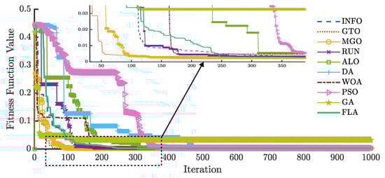
Figure 22. RMSE evolution of different algorithms for the PVM using $Ob{j}_1$.

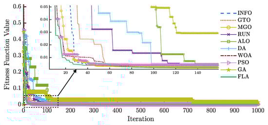
Figure 23. RMSE evolution of different algorithms for the PVM using $Ob{j}_2$.

Figure 24 shows the convergence curves of the FLA in the case of the PVM for $Ob{j}_1$ and $Ob{j}_2$. $Ob{j}_1$ converges to the lowest value at iteration 250. However, $Ob{j}_2$ converges around iteration 30, which proves the effectiveness of using $Ob{j}_2$ in the case of PVM.

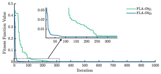
Figure 24. RMSE evolution of the FLA for the PVM using $Ob{j}_1$ and $Ob{j}_2$.

Figure 25 illustrates the relative error values $R_e$ of the simulated and experimental current data using the FLA for Photowatt-PWP201.

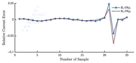
Figure 25. The relative error values of the simulated current data and the experimental current data using the FLA for Photowatt-PWP201.

Figure 26 illustrates the current–voltage and power–voltage characteristic curves with the FLA for Photowatt-PWP201 using $Ob{j}_1$ and $Ob{j}_2$. As remarked, the estimated data based on $Ob{j}_2$ are closer to the experimental data than the data based on $Ob{j}_1$; this again proves the superiority of using $Ob{j}_2$ over $Ob{j}_1$.

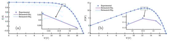
Figure 26. The (a) I-V and (b) P-V curves of the FLA for Photowatt-PWP201, using $Ob{j}_1$ and $Ob{j}_2$.

7. Conclusions and Future Directions

Accurately estimating the parameters of a solar panel increases the system’s efficiency and assists with the design of advanced control systems. Advances in modeling methodologies and algorithms can lead to more accurate, scalable, and cost-effective solutions for the solar energy sector.

In this study, a metaheuristic algorithm, the flood algorithm (FLA), inspired by flood phenomena, was employed to identify the parameters of different photovoltaic models. The FLA was applied to single-diode, double-diode, and three-diode PV cells, as well as a single-diode PV module model. This study used the RTC France cell and Photowatt-PWP201 module as benchmarks. Two objective functions based on two approaches were used to formulate the optimization problem. The results of the FLA were compared with nine well-known metaheuristic algorithms. The findings demonstrate the FLA’s superiority over other algorithms and highlight the utility of integrating the Newton–Raphson method in formulating the objective function. Additionally, the three-diode PV cell model illustrates the effectiveness of this approach in representing the RTC France solar cell.

Applying the FLA for the SDM, DDM, and TDM of RTC France demonstrates their effectiveness, achieving an RMSE of $9.8034\times {10}^{-4}$ for the TDM using $Ob{j}_1$ and $7.3652\times {10}^{-4}$ using $Ob{j}_2$, signifying that the TDM is the best model to represent the RTC France solar cell. Moreover, the comparison between various algorithms for the PVM in the Photowatt-PWP201 module confirms that the FLA, INFO, and GTO algorithms are the most effective for this model, delivering the lowest RMSE values among the employed algorithms. On the other hand, modifying the first objective function $Ob{j}_1$ by integrating the Newton–Raphson method results in faster convergence and a lower RMSE for all tested algorithms. However, the computational costs are significantly higher for $Ob{j}_2$, which is the primary drawback of this approach.

Future research could focus on the following:

• Enhancing the convergence speed of the Newton–Raphson integration. Modifying the FLA by incorporating the Newton–Raphson method may further accelerate convergence and reduce computational costs.
• Performing in-depth analysis of the temporal and spatial complexity of metaheuristic algorithms applied for photovoltaic parameter extraction.
• Conducting non-parametric studies, such as the Wilcoxon test, which would further strengthen the statistical robustness of metaheuristic algorithms for photovoltaic parameter extraction and provide deeper insights into the variability and reliability of the different methods.

References

- Abas, N.; Kalair, A.; Khan, N. Review of fossil fuels and future energy technologies. Futures 2015, 69, 31–49. [Google Scholar] [CrossRef]
- Holechek, J.L.; Geli, H.M.E.; Sawalhah, M.N.; Valdez, R. A Global Assessment: Can Renewable Energy Replace Fossil Fuels by 2050? Sustainability 2022, 14, 4792. [Google Scholar] [CrossRef]
- York, R.; Bell, S.E. Energy transitions or additions? Energy Res. Soc. Sci. 2019, 51, 40–43. [Google Scholar] [CrossRef]
- Mansuri, M.F.; Saxena, B.K.; Mishra, S. Shifting from Fossil Fuel Vehicles to H2 based Fuel Cell Electric Vehicles: Case Study of a Smart City. In Proceedings of the 2020 International Conference on Advances in Computing, Communication & Materials (ICACCM), Dehradun, India, 21–22 August 2020; Volume 3, pp. 316–321. [Google Scholar] [CrossRef]
- Mutezo, G.; Mulopo, J. A review of Africa’s transition from fossil fuels to renewable energy using circular economy principles. Renew. Sustain. Energy Rev. 2021, 137, 110609. [Google Scholar] [CrossRef]
- Khare, V.; Nema, S.; Baredar, P. Solar–wind hybrid renewable energy system: A review. Renew. Sustain. Energy Rev. 2016, 58, 23–33. [Google Scholar] [CrossRef]
- Pandey, A.; Tyagi, V.; Selvaraj, J.A.; Rahim, N.; Tyagi, S. Recent advances in solar photovoltaic systems for emerging trends and advanced applications. Renew. Sustain. Energy Rev. 2016, 53, 859–884. [Google Scholar] [CrossRef]
- Hernández-Callejo, L.; Gallardo-Saavedra, S.; Alonso-Gómez, V. A review of photovoltaic systems: Design, operation and maintenance. Sol. Energy 2019, 188, 426–440. [Google Scholar] [CrossRef]
- Nikhil, P.G.; Subhakar, D. An improved simulation model for photovoltaic cell. In Proceedings of the 2011 International Conference on Electrical and Control Engineering, Yichang, China, 16–18 September 2011; Volume 146, pp. 1978–1982. [Google Scholar] [CrossRef]
- Morcillo-Herrera, C.; Hernández-Sánchez, F.; Flota-Bañuelos, M. Method to Calculate the Electricity Generated by a Photovoltaic Cell, Based on Its Mathematical Model Simulations in MATLAB. Int. J. Photoenergy 2015, 2015, 545831. [Google Scholar] [CrossRef]
- Nguyen, X.H.; Nguyen, M.P. Mathematical modeling of photovoltaic cell/module/arrays with tags in Matlab/Simulink. Environ. Syst. Res. 2015, 4, 24. [Google Scholar] [CrossRef]
- Ahmad, T.; Sobhan, S.; Nayan, M.F. Comparative Analysis between Single Diode and Double Diode Model of PV Cell: Concentrate Different Parameters Effect on Its Efficiency. J. Power Energy Eng. 2016, 4, 31–46. [Google Scholar] [CrossRef]
- Jain, A. Exact analytical solutions of the parameters of real solar cells using Lambert W-function. Sol. Energy Mater. Sol. Cells 2004, 81, 269–277. [Google Scholar] [CrossRef]
- Jain, A.; Sharma, S.; Kapoor, A. Solar cell array parameters using Lambert W-function. Sol. Energy Mater. Sol. Cells 2006, 90, 25–31. [Google Scholar] [CrossRef]
- Tripathy, M.; Kumar, M.; Sadhu, P. Photovoltaic system using Lambert W function-based technique. Sol. Energy 2017, 158, 432–439. [Google Scholar] [CrossRef]
- Cardenas, A.A.; Carrasco, M.; Mancilla-David, F.; Street, A.; Cardenas, R. Experimental Parameter Extraction in the Single-Diode Photovoltaic Model via a Reduced-Space Search. IEEE Trans. Ind. Electron. 2017, 64, 1468–1476. [Google Scholar] [CrossRef]
- Yetayew, T.T.; Jyothsna, T.R. Parameter extraction of photovoltaic modules using Newton Raphson and simulated annealing techniques. In Proceedings of the 2015 IEEE Power, Communication and Information Technology Conference (PCITC), Bhubaneswar, India, 15–17 October 2015; pp. 229–234. [Google Scholar] [CrossRef]
- Nunes, H.; Pombo, J.; Mariano, S.; do Rosario Calado, M. Newton-Raphson method versus Lambert W function for photovoltaic parameter estimation. In Proceedings of the 2022 IEEE International Conference on Environment and Electrical Engineering and 2022 IEEE Industrial and Commercial Power Systems Europe (EEEIC & CPS Europe), Prague, Czech Republic, 28 June–1 July 2022; pp. 1–6. [Google Scholar] [CrossRef]
- Et-torabi, K.; Nassar-eddine, I.; Obbadi, A.; Errami, Y.; Rmaily, R.; Sahnoun, S.; El fajri, A.; Agunaou, M. Parameters estimation of the single and double diode photovoltaic models using a Gauss–Seidel algorithm and analytical method: A comparative study. Energy Convers. Manag. 2017, 148, 1041–1054. [Google Scholar] [CrossRef]
- Babu, T.; Kumar, N.P. Iterative Based Parameter Estimation for Non-Linear Model of a PV Module. Int. J. Eng. Adv. Technol. 2019, 8, 788–791. [Google Scholar] [CrossRef]
- Mesbahi, O.; Tlemçani, M.; Janeiro, F.M.; Hajjaji, A.; Kandoussi, K. Sensitivity analysis of a new approach to photovoltaic parameters extraction based on the total least squares method. Metrol. Meas. Syst. 2021, 28, 751–765. [Google Scholar] [CrossRef]
- Mesbahi, O.; Tlemçani, M.; Janeiro, F.M.; Hajjaji, A.; Kandoussi, K. Recent Development on Photovoltaic Parameters Estimation: Total Least Squares Approach and Metaheuristic Algorithms. Energy Sources Part A Recover. Util. Environ. Eff. 2022, 44, 4546–4564. [Google Scholar] [CrossRef]
- Ismail, M.; Moghavvemi, M.; Mahlia, T. Characterization of PV panel and global optimization of its model parameters using genetic algorithm. Energy Convers. Manag. 2013, 73, 10–25. [Google Scholar] [CrossRef]
- Ma, J.; Man, K.L.; Guan, S.U.; Ting, T.O.; Wong, P.W.H. Parameter estimation of photovoltaic model via parallel particle swarm optimization algorithm: Parallel particle swarm optimization. Int. J. Energy Res. 2015, 40, 343–352. [Google Scholar] [CrossRef]
- Ebrahimi, S.M.; Salahshour, E.; Malekzadeh, M.; Gordillo, F. Parameters identification of PV solar cells and modules using flexible particle swarm optimization algorithm. Energy 2019, 179, 358–372. [Google Scholar] [CrossRef]
- Xu, S.; Wang, Y. Parameter estimation of photovoltaic modules using a hybrid flower pollination algorithm. Energy Convers. Manag. 2017, 144, 53–68. [Google Scholar] [CrossRef]
- Kang, T.; Yao, J.; Jin, M.; Yang, S.; Duong, T. A Novel Improved Cuckoo Search Algorithm for Parameter Estimation of Photovoltaic (PV) Models. Energies 2018, 11, 1060. [Google Scholar] [CrossRef]
- Deotti, L.M.P.; Pereira, J.L.R.; Silva Júnior, I.C.d. Parameter extraction of photovoltaic models using an enhanced Lévy flight bat algorithm. Energy Convers. Manag. 2020, 221, 113114. [Google Scholar] [CrossRef]
- Diab, A.A.Z.; Sultan, H.M.; Aljendy, R.; Al-Sumaiti, A.S.; Shoyama, M.; Ali, Z.M. Tree Growth Based Optimization Algorithm for Parameter Extraction of Different Models of Photovoltaic Cells and Modules. IEEE Access 2020, 8, 119668–119687. [Google Scholar] [CrossRef]
- Naeijian, M.; Rahimnejad, A.; Ebrahimi, S.M.; Pourmousa, N.; Gadsden, S.A. Parameter estimation of PV solar cells and modules using Whippy Harris Hawks Optimization Algorithm. Energy Rep. 2021, 7, 4047–4063. [Google Scholar] [CrossRef]
- Shaban, H.; Houssein, E.H.; Pérez-Cisneros, M.; Oliva, D.; Hassan, A.Y.; Ismaeel, A.A.K.; AbdElminaam, D.S.; Deb, S.; Said, M. Identification of Parameters in Photovoltaic Models through a Runge Kutta Optimizer. Mathematics 2021, 9, 2313. [Google Scholar] [CrossRef]
- Xiong, G.; Li, L.; Mohamed, A.W.; Yuan, X.; Zhang, J. A new method for parameter extraction of solar photovoltaic models using gaining sharing knowledge based algorithm. Energy Rep. 2021, 7, 3286–3301. [Google Scholar] [CrossRef]
- Sharma, A.; Dasgotra, A.; Tiwari, S.K.; Sharma, A.; Jately, V.; Azzopardi, B. Parameter Extraction of Photovoltaic Module Using Tunicate Swarm Algorithm. Electronics 2021, 10, 878. [Google Scholar] [CrossRef]
- Hamadi, S.A.; Chouder, A.; Rezaoui, M.M.; Motahhir, S.; Kaddouri, A.M. Improved Hybrid Parameters Extraction of a PV Module Using a Moth Flame Algorithm. Electronics 2021, 10, 2798. [Google Scholar] [CrossRef]
- Ayyarao, T.L.V.; Kumar, P.P. Parameter estimation of solar <scp>PV</scp> models with a new proposed war strategy optimization algorithm. Int. J. Energy Res. 2022, 46, 7215–7238. [Google Scholar] [CrossRef]
- Demirtas, M.; Koc, K. Parameter Extraction of Photovoltaic Cells and Modules by INFO Algorithm. IEEE Access 2022, 10, 87022–87052. [Google Scholar] [CrossRef]
- Duan, Z.; Yu, H.; Zhang, Q.; Tian, L. Parameter Extraction of Solar Photovoltaic Model Based on Nutcracker Optimization Algorithm. Appl. Sci. 2023, 13, 6710. [Google Scholar] [CrossRef]
- Moustafa, G. Parameter Identification of Solar Photovoltaic Systems Using an Augmented Subtraction-Average-Based Optimizer. Eng 2023, 4, 1818–1836. [Google Scholar] [CrossRef]
- Abd El-Mageed, A.A.; Abohany, A.A.; Saad, H.M.; Sallam, K.M. Parameter extraction of solar photovoltaic models using queuing search optimization and differential evolution. Appl. Soft Comput. 2023, 134, 110032. [Google Scholar] [CrossRef]
- Abbassi, R.; Saidi, S.; Urooj, S.; Alhasnawi, B.N.; Alawad, M.A.; Premkumar, M. An Accurate Metaheuristic Mountain Gazelle Optimizer for Parameter Estimation of Single- and Double-Diode Photovoltaic Cell Models. Mathematics 2023, 11, 4565. [Google Scholar] [CrossRef]
- Rai, N.; Abbadi, A.; Hamidia, F.; Douifi, N.; Abdul Samad, B.; Yahya, K. Biogeography-Based Teaching Learning-Based Optimization Algorithm for Identifying One-Diode, Two-Diode and Three-Diode Models of Photovoltaic Cell and Module. Mathematics 2023, 11, 1861. [Google Scholar] [CrossRef]
- Kullampalayam Murugaiyan, N.; Chandrasekaran, K.; Manoharan, P.; Derebew, B. Leveraging opposition-based learning for solar photovoltaic model parameter estimation with exponential distribution optimization algorithm. Sci. Rep. 2024, 14, 528. [Google Scholar] [CrossRef] [PubMed]
- Li, Y.; Xiong, G.; Mirjalili, S.; Wagdy Mohamed, A. Optimal equivalent circuit models for photovoltaic cells and modules using multi-source guided teaching–learning-based optimization. Ain Shams Eng. J. 2024, 15, 102988. [Google Scholar] [CrossRef]
- Ajay Rathod, A.; Subramanian, B. Efficient approach for optimal parameter estimation of PV using Pelican Optimization Algorithm. Cogent Eng. 2024, 11, 2380805. [Google Scholar] [CrossRef]
- Yaghoubi, M.; Eslami, M.; Noroozi, M.; Mohammadi, H.; Kamari, O.; Palani, S. Modified Salp Swarm Optimization for Parameter Estimation of Solar PV Models. IEEE Access 2022, 10, 110181–110194. [Google Scholar] [CrossRef]
- Li, S.; Gu, Q.; Gong, W.; Ning, B. An enhanced adaptive differential evolution algorithm for parameter extraction of photovoltaic models. Energy Convers. Manag. 2020, 205, 112443. [Google Scholar] [CrossRef]
- Shaheen, A.M.; Ginidi, A.R.; El-Sehiemy, R.A.; Ghoneim, S.S.M. A Forensic-Based Investigation Algorithm for Parameter Extraction of Solar Cell Models. IEEE Access 2021, 9, 1–20. [Google Scholar] [CrossRef]
- Zhang, Y.; Ma, M.; Jin, Z. Comprehensive learning Jaya algorithm for parameter extraction of photovoltaic models. Energy 2020, 211, 118644. [Google Scholar] [CrossRef]
- Fan, Y.; Wang, P.; Heidari, A.A.; Zhao, X.; Turabieh, H.; Chen, H. Delayed dynamic step shuffling frog-leaping algorithm for optimal design of photovoltaic models. Energy Rep. 2021, 7, 228–246. [Google Scholar] [CrossRef]
- Xiong, G.; Zhang, J.; Shi, D.; Zhu, L.; Yuan, X. Parameter extraction of solar photovoltaic models with an either-or teaching learning based algorithm. Energy Convers. Manag. 2020, 224, 113395. [Google Scholar] [CrossRef]
- Wolpert, D.; Macready, W. No free lunch theorems for optimization. IEEE Trans. Evol. Comput. 1997, 1, 67–82. [Google Scholar] [CrossRef]
- Ghasemi, M.; Golalipour, K.; Zare, M.; Mirjalili, S.; Trojovský, P.; Abualigah, L.; Hemmati, R. Flood algorithm (FLA): An efficient inspired meta-heuristic for engineering optimization. J. Supercomput. 2024, 80, 22913–23017. [Google Scholar] [CrossRef]
- Gomes, R.C.M.; Vitorino, M.A.; Correa, M.B.R.; Wang, R.; Fernandes, D.A. Photovoltaic parameter extraction using Shuffled Complex Evolution. In Proceedings of the 2015 IEEE 13th Brazilian Power Electronics Conference and 1st Southern Power Electronics Conference (COBEP/SPEC), Fortaleza, Brazil, 29 November–2 December 2015; pp. 1–6. [Google Scholar] [CrossRef]
- Liang, J.; Qiao, K.; Yuan, M.; Yu, K.; Qu, B.; Ge, S.; Li, Y.; Chen, G. Evolutionary multi-task optimization for parameters extraction of photovoltaic models. Energy Convers. Manag. 2020, 207, 112509. [Google Scholar] [CrossRef]
- Alanazi, M.; Alanazi, A.; Almadhor, A.; Rauf, H.T. Photovoltaic Models’ Parameter Extraction Using New Artificial Parameterless Optimization Algorithm. Mathematics 2022, 10, 4617. [Google Scholar] [CrossRef]
- Long, W.; Cai, S.; Jiao, J.; Xu, M.; Wu, T. A new hybrid algorithm based on grey wolf optimizer and cuckoo search for parameter extraction of solar photovoltaic models. Energy Convers. Manag. 2020, 203, 112243. [Google Scholar] [CrossRef]
- Weng, X.; Heidari, A.A.; Liang, G.; Chen, H.; Ma, X.; Mafarja, M.; Turabieh, H. Laplacian Nelder-Mead spherical evolution for parameter estimation of photovoltaic models. Energy Convers. Manag. 2021, 243, 114223. [Google Scholar] [CrossRef]
- Shaheen, A.M.; Elsayed, A.M.; Ginidi, A.R.; El-Sehiemy, R.A.; Elattar, E. Enhanced social network search algorithm with powerful exploitation strategy for PV parameters estimation. Energy Sci. Eng. 2022, 10, 1398–1417. [Google Scholar] [CrossRef]
- Li, S.; Gong, W.; Wang, L.; Yan, X.; Hu, C. A hybrid adaptive teaching–learning-based optimization and differential evolution for parameter identification of photovoltaic models. Energy Convers. Manag. 2020, 225, 113474. [Google Scholar] [CrossRef]
- Ismaeel, A.A.K.; Houssein, E.H.; Oliva, D.; Said, M. Gradient-Based Optimizer for Parameter Extraction in Photovoltaic Models. IEEE Access 2021, 9, 13403–13416. [Google Scholar] [CrossRef]
- Beşkirli, A.; Dağ, D. Parameter extraction for photovoltaic models with tree seed algorithm. Energy Rep. 2023, 9, 174–185. [Google Scholar] [CrossRef]
- Ahmadianfar, I.; Heidari, A.A.; Noshadian, S.; Chen, H.; Gandomi, A.H. INFO: An efficient optimization algorithm based on weighted mean of vectors. Expert Syst. Appl. 2022, 195, 116516. [Google Scholar] [CrossRef]
- Abdollahzadeh, B.; Soleimanian Gharehchopogh, F.; Mirjalili, S. Artificial gorilla troops optimizer: A new nature-inspired metaheuristic algorithm for global optimization problems. Int. J. Intell. Syst. 2021, 36, 5887–5958. [Google Scholar] [CrossRef]
- Abdollahzadeh, B.; Gharehchopogh, F.S.; Khodadadi, N.; Mirjalili, S. Mountain Gazelle Optimizer: A new Nature-inspired Metaheuristic Algorithm for Global Optimization Problems. Adv. Eng. Softw. 2022, 174, 103282. [Google Scholar] [CrossRef]
- Ahmadianfar, I.; Heidari, A.A.; Gandomi, A.H.; Chu, X.; Chen, H. RUN beyond the metaphor: An efficient optimization algorithm based on Runge Kutta method. Expert Syst. Appl. 2021, 181, 115079. [Google Scholar] [CrossRef]
- Mirjalili, S. The Ant Lion Optimizer. Adv. Eng. Softw. 2015, 83, 80–98. [Google Scholar] [CrossRef]
- Mirjalili, S. Dragonfly algorithm: A new meta-heuristic optimization technique for solving single-objective, discrete, and multi-objective problems. Neural Comput. Appl. 2015, 27, 1053–1073. [Google Scholar] [CrossRef]
- Mirjalili, S.; Lewis, A. The Whale Optimization Algorithm. Adv. Eng. Softw. 2016, 95, 51–67. [Google Scholar] [CrossRef]
- Kennedy, J.; Eberhart, R. Particle swarm optimization. In Proceedings of the ICNN’95—International Conference on Neural Networks, Perth, WA, Australia, 27 November–1 December 1995; Volume 4, pp. 1942–1948. [Google Scholar] [CrossRef]
- Katoch, S.; Chauhan, S.S.; Kumar, V. A review on genetic algorithm: Past, present, and future. Multimed. Tools Appl. 2020, 80, 8091–8126. [Google Scholar] [CrossRef] [PubMed]
Disclaimer/Publisher’s Note: The statements, opinions and data contained in all publications are solely those of the individual author(s) and contributor(s) and not of MDPI and/or the editor(s). MDPI and/or the editor(s) disclaim responsibility for any injury to people or property resulting from any ideas, methods, instructions or products referred to in the content. |
© 2024 by the authors. Licensee MDPI, Basel, Switzerland. This article is an open access article distributed under the terms and conditions of the Creative Commons Attribution (CC BY) license (https://creativecommons.org/licenses/by/4.0/).