Enhanced Small Reflections Sparse-Spike Seismic Inversion with Iterative Hybrid Thresholding Algorithm

Abstract

Seismic inversion is a process of imaging or predicting the spatial and physical properties of underground strata. The most commonly used one is sparse-spike seismic inversion with sparse regularization. There are many effective methods to solve sparse regularization, such as L0-norm, L1-norm, weighted L1-norm, etc. This paper studies the sparse-spike inversion with L0-norm. It is usually solved by the iterative hard thresholding algorithm (IHTA) or its faster variants. However, hard thresholding algorithms often lead to a sharp increase or numerical oscillation of the residual, which will affect the inversion results. In order to deal with this issue, this paper attempts the idea of the relaxed optimal thresholding algorithm (ROTA). In the solution process, due to the particularity of the sparse constraints in this convex relaxation model, this model can be considered as a L1-norm problem when dealt with the location of non-zero elements. We use a modified iterative soft thresholding algorithm (MISTA) to solve it. Hence, it forms a new algorithm called the iterative hybrid thresholding algorithm (IHyTA), which combines IHTA and MISTA. The synthetic and real seismic data tests show that, compared with IHTA, the results of IHyTA are more accurate with the same SNR. IHyTA improves the noise resistance.

1. Introduction

Seismic inversion is widely used in stratum analysis, oil and gas exploration, and seismic monitoring, and is the core technology of reservoir prediction. The wave impedance of strata is the result of post-stack seismic inversion, which can reflect the physical characteristics of rock formation, and is one of the most widely used parameters in reservoir prediction and reservoir characteristic description.

In seismic inversion, the seismic data is first inverted to obtain the reflectivity sequence of the underground strata. Then, under an exponential integral transformation, the final impedance can be found according to the resulting reflectivity series [1,2]. Thus, the quality of the estimated impedance is directly influenced by the quality of the reflectivity sequence. In seismology, the observed seismic data is considered as the result from the convolution between the reflectivity series and the seismic wavelet. Thus, the reflectivity series inversion is in fact a deconvolution problem, which is an ill-posed inverse problem. In order to deal with the ill-posedness, the most effective method is to perform regularization [3,4].

In practice, there is a lot of noise when observing or processing the real seismic data. Here, the real seismic data is expressed as the addition of synthetic seismic data from reflectivity series and random noise.

From the convolution model of seismic data, it can be written as d(t) = w(t)*r(t) + n(t) [3], where d(t) is the observed seismic signal, w(t) is the seismic wavelet, r(t) is the reflectivity series of underground, t is the travel time of seismic wave, and n(t) is the noise in seismic data. In discrete format, it can be expressed as [3],

$$d=Gr+n.$$

(1)

Here, G is the forward operator from convolution, d is the seismic data, r is the reflectivity series, and n is the random noise.

Seismic inversion is considerably affected by seismic observation noise. The inversion results are often unstable, which means a small amount of noise can make the inversion results produce a strong disturbance. Therefore, regularization and other a priori information should be added as constraints in the inversion process to ensure the reliability of the inversion results [5]. One of the commonly used in seismic inversion is sparse regularization. It is called sparse-spike inversion. The principle is to assume that the reflectivity series of underground formations is to superposition a series of strong reflections, which is sparse distributed and small reflection coefficient. And the seismic wavelet is estimated through different methods. Then the spike-like reflection coefficient series is obtained based on deconvolution of seismic data with sparse regularization. Finally, the reflection coefficient series is recursively inverted to generate the impedance of underground formation.

The seismic deconvolution with L0-norm sparse regularization can be expressed as,

$$\underset{r}{\min }\left|\right|r|{|}_0,\mathrm{s}.\mathrm{t}.||d-Gr|{|}_2^2\le \epsilon ,$$

(2)

where, $\left|\right|.|{|}_0$ is the so-called L0-norm of vector, it is actually the number of non-zero elements, and $\left|\right|.|{|}_2$ is the L2-norm of vector. Such L0-norm minimization linear inverse problems are NP-hard [6]. It is to find the sparsest solution of r, which can obtain a synthetic seismic data to match the observed seismic data.

A commonly used approaches to solve the L0-nom sparse regularization inverse problem is iterative thresholding algorithms. The most basic algorithms in this category are the iterative hard thresholding algorithm (IHTA) [7] and its fast version, i.e., fast iterative hard thresholding algorithm (FIHTA) [8].

The sparse regularization can not only make the inversion result more stable, but can also better describe the nature of sparsity of seismic data and model parameters. There are many effective candidates to perform sparse regularization, such as L0-norm [9], L1-norm [10], weighted L1-norm regularization [11], Cauchy regularization [12], modified Cauchy regularization [13], and so forth. Sacchi studied Cauchy regularization to improve the deconvolution of seismography and successfully retrieved the sparse reflectivity series with broadband [14]. Zhang and Dai employed a modified Cauchy regularization method in the nonlinear pre-stack seismic inversion and employed a variable measure algorithm to solve it [15]. Aravkin et al. used the t regularization method based on student distribution for robust seismic data processing and inversion [16]. Li and Zhang proposed an amplitude inversion of pre-stack seismic data based on total variation regularization, which is in fact the L1-norm regularization of model parameters’ gradient [17]. Candes et al. proposed a modified L1-norm regularization, i.e., weighted L1-norm regularization to enhance sparsity when the problem to be solved exists degeneracy [11]. Since the L0-norm has an optimal sparsity compared to other sparse regularization, Dai and Yang use it as a regularization of the seismic inversion [18].

However, empirical data show that IHTA is actually inefficient and is strict with G. To solve this problem, Forcart [19] proposed hard thresholding pursuit (HTP), but the experiment shows that the residuals at the iterations generated by HTP may still oscillate significantly. This is because the hard thresholding operators tend to increase the residue rather than decrease. To deal with the oscillation issue, Zhao [20] et al. explored the optimal thresholding algorithm (OTA), combined the thresholding with the residual reduction, and further proposed the optimal thresholding pursuit algorithm (OTPA). Moreover, because OTA and OTPA are binary quadratic problems, which are not easy to solve directly, the relaxed optimal thresholding algorithm (ROTA) and the relaxed optimal thresholding pursuit (ROTPA) are proposed in the same paper. Unlike IHTA or FIHTA, which directly perform the hard thresholding algorithm on the largest non-zero elements, he adopted a sub-problem to find the locations of optimal non-zero elements to keep the residue non-increase. From Zhao’s research [20], it indicates that when the hard thresholding is applied on local dense vectors (but global sparse), the residue will oscillate significantly. In his methods, alternative compressible vectors, which are optimal from the solution of sub-problem to find the locations of optimal non-zero elements, are selected to avoid oscillation and loss of large amounts of information from small elements. The property of these algorithms proposed by Zhao is important for seismic inversion. The local dense reflectivity series often represents local small reflections. Hence, the conventional IHTA will suppress these small reflectivity series.

In this paper, we inherit the basic idea of Zhao’s paper to solve the sparse-spike seismic inversion. But in his paper, he used interior point method to solve the sub-problem of finding the locations of optimal non-zero elements. It is expounded that it is very time-consuming [21]. Here, we formulate this sub-problem as a L1-norm regularized problem and use a modified iterative soft thresholding algorithm (MISTA) to solve it. Hence, it forms a hybrid thresholding algorithm (IHyTA), which combines the IHTA and the ISTA. It not only overcomes the disadvantage of numerical oscillation caused by hard thresholding in the calculation process, thus making the inversion results more reliable, but also avoids the time-consuming of OTP. In Section 2.1 below, the specific solution process of IHyTA is given. In Section 2.2, considering the characteristics of the seismic data, we add the a priori low-frequency constraint to objective function of seismic inversion and deform it to a unify form. In Section 2.3, we give specific procedures with IHyTA to solve the objective function of sparse-spike inversion. In Section 3.1 and Section 3.2, the proposed algorithm is compared to IHTA by using a synthetic seismic trace and a 3D real seismic data volume to demonstrate its efficacy in solving sparse-spike inversion, respectively. It confirms that IHyTA protects some small reflectivity series to some extents and obtains more accurate inversion results with the same SNR. Finally, we perform some discussions in Section 4 and conclude in Section 5.

2. Methods

2.1. Iterative Hybrid Thresholding Algorithm

In inverse problem, the Equation (2) can be equivalently written as [3],

$$\underset{r}{\min }f(r)={‖d-Gr‖}_2^2+\lambda {‖r‖}_0,$$

(3)

where, d∈Rⁿ, G∈R^n×m, r∈R^m, and λ is the regularization parameter of L0-norm.

From Zhao’s paper, the iterative procedures of OTP to solve Equation (3) can be described as:

• At the kth iteration, calculate

  $$u^k=r^k+G^T(d-G{r}^k),$$

  (4)

  G^T is the transpose of G.
• Solve the sub-problem to find the locations of optimal non-zero elements:

  $$\underset{w}{\min }f(w)={‖d-G(u^k\otimes w)‖}_2^2+\lambda {‖w‖}_0,w(i)\in \{0,1\},$$

  (5)

  where w(i) is the ith elements of w, $\otimes$ is the Hadamard product of two vectors, and w is an auxiliary variable to represent the locations of non-zero elements of r. From Equation (5), the locations of non-zero elements of its solution are optimal from the view of non-increase of residue.
• Let w^k is solution of Equation (5), and set,

  $$r^{k+1}=u^k\otimes w^k,$$

  (6)

Hence, $r^{k+1}$ is the updating of r at the kth iteration. In fact, due to the elements of w (0 or 1), it is Hard thresholding with w^k.

Equation (5) is a binary optimization problem and is known to be NP-hard [22]. To find its solution, one can relax it to a convex optimization problem. This will lead to the so-called ROT [23].

Because the elements of w are 0 or 1, Equation (5) can be written as:

$$\underset{w}{\min }f(w)={‖d-G(u^k\otimes w)‖}_2^2+\lambda {‖w‖}_1,w(i)\in \{0,1\},$$

(7)

where ${‖w‖}_1$ is the L1-norm of w.

From [20], the optimal convex relaxation counterpart of Equation (7) is:

$$\underset{w}{\min }f(w)={‖d-G(u^k\otimes w)‖}_2^2+\lambda {‖w‖}_1,w(i)\in [0,1],$$

(8)

The above Equation (8) is the sub-problem to find the locations of optimal non-zero elements in ROT. In Zhao’s paper, he used interior point method to solve it. It is very time-consuming [20].

Here, we equivalently transform Equation (8). From the specifics of matrix multiplication and Hadamard product, Equation (8) can be written as:

$$\underset{w}{\min }f(w)={‖d-\stackrel{\sim }{G}w‖}_2^2+\lambda {‖w‖}_1,w(i)\in [0,1],$$

(9)

where

$$\stackrel{\sim }{G}=\left[\begin{array}{cccc}{g}_{1,1}{u}_1^k& g_{1,2}{u}_2^k& \cdots & g_{1,m}{u}_m^k\\ ⋮& ⋮& \cdots & ⋮\\ g_{n,1}{u}_1^k& g_{n,2}{u}_2^k& \cdots & g_{n,m}{u}_m^k\end{array}\right].$$

(10)

Here, g_i,j is the element of G at ith row and jth column, and $u_j^k$ is jth element of u^k.

Equation (9) is a L1-norm regularized linear inverse problem with a bound constraint. Here, we use a modified iterative soft thresholding algorithm to solve it. The specific formula is:

$$w^k(i)=\left\{\begin{array}{l}0,\begin{array}{c}\end{array}{v}^k(i)<\lambda /t\\ v^k(i)-\lambda /t,\begin{array}{c}\end{array}\lambda /t\le v^k(i)<1\\ 1,\begin{array}{c}\begin{array}{c}\end{array}{v}^k(i)\ge 1\end{array}\end{array}\right.,$$

(11)

where w^k(i) is the ith elements of w^k, v^k(i) is the ith elements of v^k, t is the largest eigenvalue of ${\stackrel{\sim }{G}}^T\stackrel{\sim }{G}$, and,

$$v^k=w^{k-1}+{\stackrel{\sim }{G}}^T(d-\stackrel{\sim }{G}{w}^{k-1}).$$

(12)

Due to that Equation (8) is the convex relaxation of Equation (7), its solution w^k may not be exactly sparse. Here, we apply the hard thresholding operator to $u^k\otimes w^k$ to obtain the updated r, i.e.,

$$r^{k+1}={\mathrm{Hard}}_{{\displaystyle \raisebox{1ex}{$\lambda $}\!\left/ \!\raisebox{-1ex}{$h$}\right.}}(u^k\otimes w^k),$$

(13)

where Hard_λ/h is the hard thresholding operator with λ/h, h is the largest eigenvalue of G^TG.

Based on the above contents, it forms a hybrid thresholding algorithm, which combines the IHTA (which updates r) and ISTA (which solves the relax version of sub-problem to find the locations of optimal non-zero elements).

2.2. Objective Function of Seismic Inversion

As usual, in the linear inverse problem, the objective function takes the form as Equation (3). Due to the lack of low-frequency information in seismic data, we add a priori model constraints into Equation (3) to ensure that the inversion results contain low-frequency components [13]. The objective function becomes:

$$\underset{r}{\min }f(r)={‖d-Gr‖}_2^2+\rho {‖Cr-\xi ‖}_2^2+\lambda {‖r‖}_0,$$

(14)

where ξ is the a priori logarithmic impedance and C is the integral operator [24].

In order to directly adopt IHyTA to solve Equation (14), we deform it to a unify form, i.e.,

$$\underset{r}{\min }f(r)={‖\left(\begin{array}{c}d\\ \sqrt{\rho }\xi \end{array}\right)-\left(\begin{array}{c}G\\ \sqrt{\rho }C\end{array}\right)r‖}_2^2+\lambda {‖r‖}_0.$$

(15)

Set

$$\tilde{d}=\left(\begin{array}{c}d\\ \sqrt{\rho }\xi \end{array}\right),A=\left(\begin{array}{c}G\\ \sqrt{\rho }C\end{array}\right),$$

(16)

then we have

$$\underset{r}{\min }f(r)={‖\tilde{d}-Ar‖}_2^2+\lambda {‖r‖}_0.$$

(17)

Equation (17) takes the same form as Equation (3).

2.3. IHyTA to Solve Sparse-Spike Seismic Inversion

From the Section 2.1 and Section 2.2, the iterative procedures of IHyTA to solve Equation (17) can be described as:

• At the kth iteration, calculate

  $$u^k=r^k+A^T(\stackrel{\sim }{d}-A{r}^k),$$

  (18)
• Calculate

  $$v^k=w^{k-1}+{\stackrel{\sim }{A}}^T(\stackrel{\sim }{d}-\stackrel{\sim }{A}{w}^{k-1}).$$

  (19)

  where,

  $$\stackrel{\sim }{A}=\left[\begin{array}{cccc}{a}_{1,1}{u}_1^k& a_{1,2}{u}_2^k& \cdots & a_{1,m}{u}_m^k\\ ⋮& ⋮& \cdots & ⋮\\ a_{n,1}{u}_1^k& a_{n,2}{u}_2^k& \cdots & a_{n,m}{u}_m^k\end{array}\right]$$

  (20)

  Here, a_i,j is the element of A at ith row and jth column.
• Calculate w^k with MISTA, i.e., Equation (11). But now, t is the largest eigenvalue of ${\stackrel{\sim }{A}}^T\stackrel{\sim }{A}$.
• Apply the hard thresholding operator to $u^k\otimes w^k$ to obtain the updated r, i.e., Equation (13). But now, h is the largest eigenvalue of $A^{T}A$.
• The pseudo code is given in Algorithm 1.

Algorithm 1. The pseudo code to obtain a new rk.

$\mathrm{Input}:\mathrm{vector}{\mathbf{u}}^k{\mathbf{v}}^k,\mathsf{\lambda }\mathrm{is}\mathrm{the}\mathrm{regularization}\mathrm{parameter}\mathrm{of}\mathrm{L}0\text{-}\mathrm{norm}.t={\mathsf{\lambda }}_{\max }\left({\stackrel{\sim }{A}}^T\stackrel{\sim }{A}\right)\mathrm{is}\mathrm{the}$$\mathrm{largest}\mathrm{eigenvalue}\mathrm{of}{\stackrel{\sim }{A}}^T\stackrel{\sim }{A}$$,h={\mathsf{\lambda }}_{\max }(A^{T}A$$)\mathrm{is}\mathrm{the}\mathrm{largest}\mathrm{eigenvalue}\mathrm{of}{A}^{T}A$. (1) for i < m (m is the length of vector uk, vkand rk) (2) $\mathrm{if}{v}^k\left(i\right)<\lambda /t$ (3) $w^k\left(i\right)=0$ (4) $\mathrm{else}\mathrm{if}{v}^k\left(i\right)<1$ (5) $w^k\left(i\right)=v^k\left(i\right)-\lambda /t$ (6) else (7) $w^k\left(i\right)=1$ (8) end for (9) $\mathrm{calculate} z^{k+1}=u^k\otimes w^k$ (10) for i < m (11) $\mathrm{if}\left|z^{k+1}\left(i\right)\right|<h\lambda$ (12) $r^{k+1}\left(i\right)=0$ (13) else (14) $r^{k+1}\left(i\right)=\left|z^{k+1}\left(i\right)\right|$ end for

3. Applications

3.1. Synthetic Seismic Data Tests

First, the feasibility of IHyTA when it is used to solve sparse-spike inversion is tested using a 1D synthetic seismic data trace. For seismic signals, an idealised model is a convolution process. The physical meaning of the convolution process is “superposition”. Consider an earth model with a layered structure. Each layer has a different acoustic impedance, which is the product of velocity and density. The contrast of acoustic impedance is called reflectivity series. Each reflectivity series as a scaling factor to scale a particular wavelet w(t), where t is the travel time. A recorded seismic trace d(t) is formed by summing all scaled wavelets reflected from different interfaces [25]. This physical process is the “superposition”, and combining all the time-shifted wavelets to form a wavelet matrix G. Then the matrix-vector form of superposition, d = Gr, is the discretized form of “convolution”.

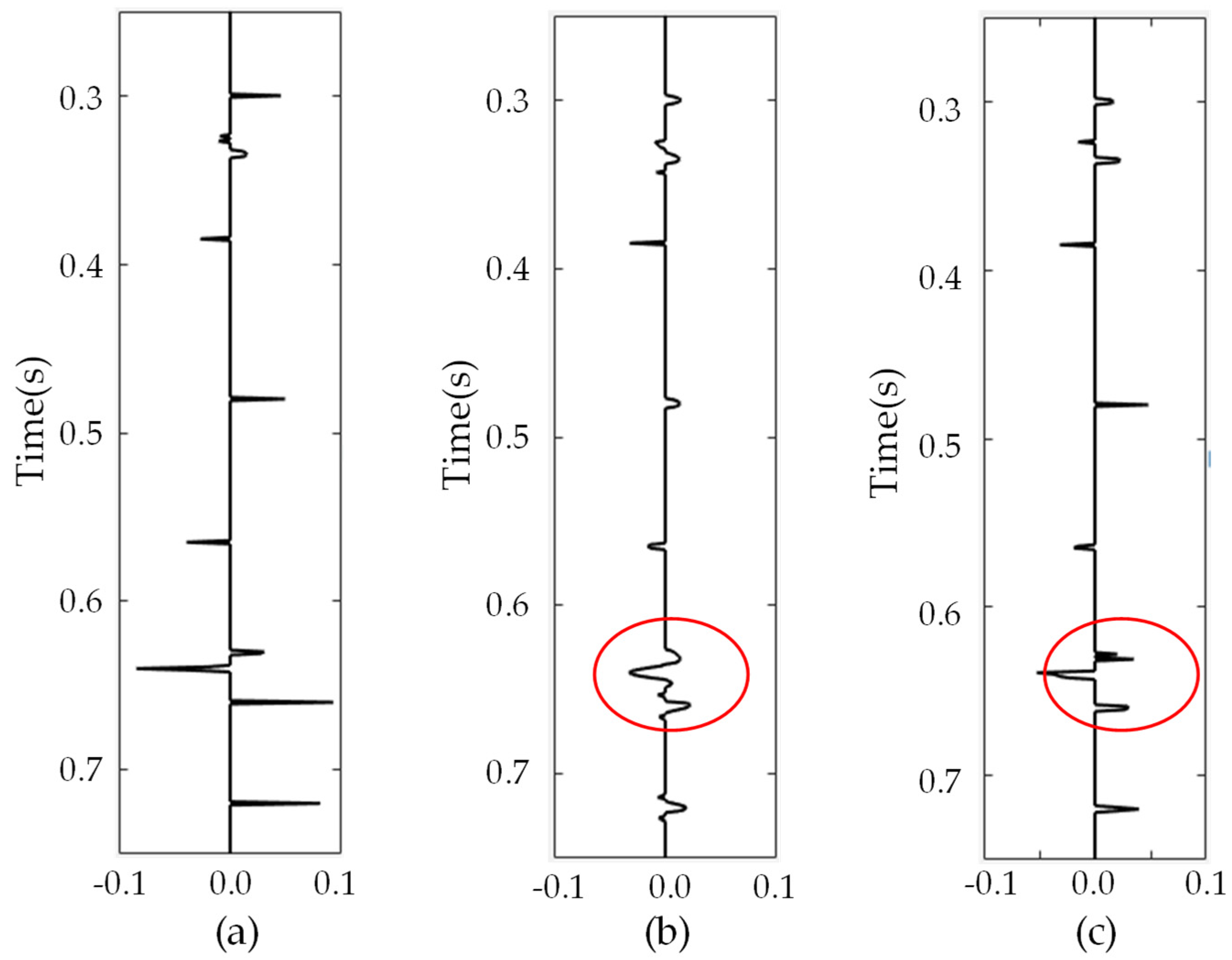
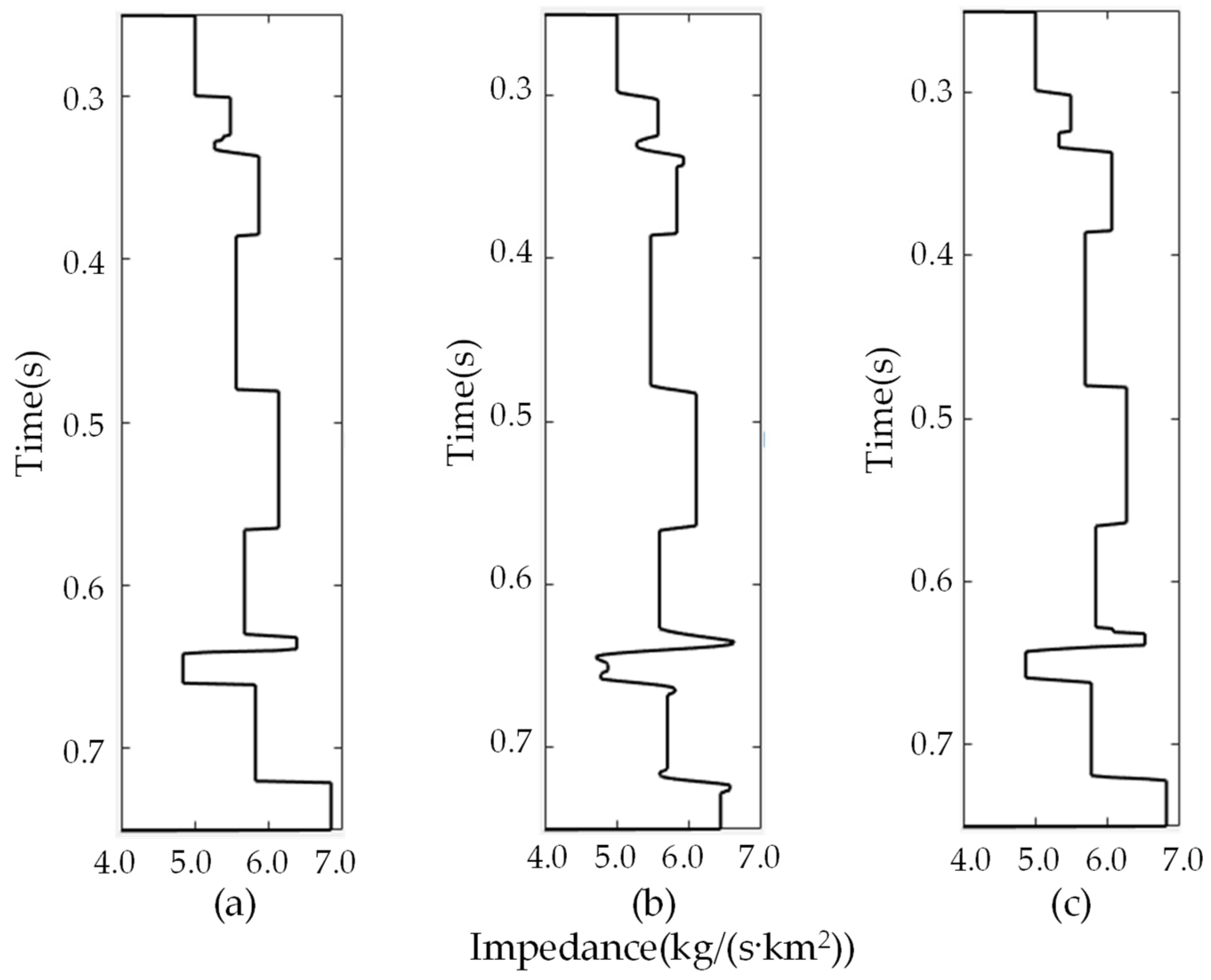
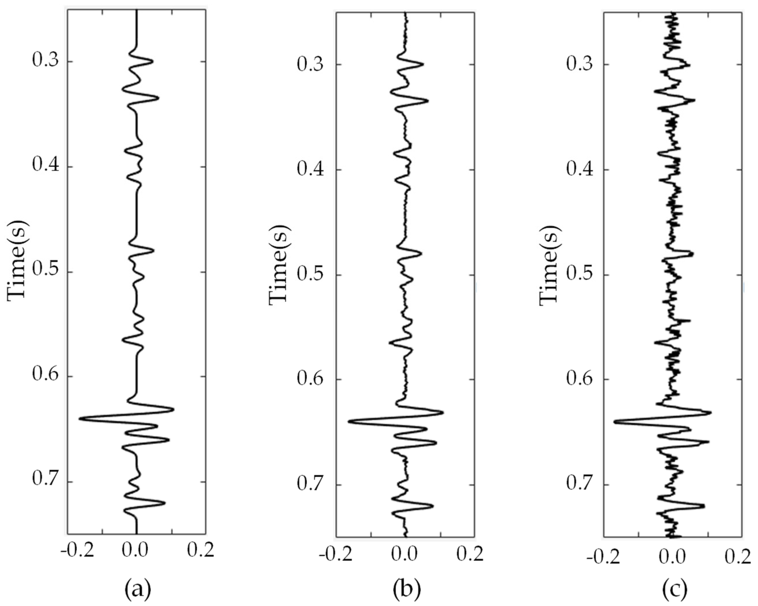
The seismic data shown in Figure 1a are obtained from the convolution of the reflectivity series in Figure 2a with the 55 Hz Ricker wavelet. The corresponding impedance model is shown in Figure 3a. Then, 5% Gaussian random noise with zero mean was added to the synthetic seismic data. The noise-contaminated seismic data is shown in Figure 1b. The sample rate is 1 ms, and the time length is 0.95s. Therefore, n = 950 in this test. From the convolution model of seismic data generation, the vertical axes of these figures are travel time of seismic wave. The horizontal axe of Figure 1 is the amplitude of seismic data; the horizontal axe of Figure 2 is the magnitude of reflectivity series; the horizontal axe of Figure 3 is the value of impedance.

Figure 1. Synthetic seismic data. (a) Noise free; (b) Noise-contaminated synthetic seismic data with 5% Gaussian random noise; (c) Noise-contaminated synthetic seismic data with 20% Gaussian random noise.

Figure 2. The true reflectivity series and inverted reflectivity series with synthetic seismic data in Figure 1b. (a) true; (b) IHTA; (c) IHyTA.

Figure 3. The true impedance and inverted impedance with synthetic seismic data in Figure 1b. (a) true; (b) IHTA; (c) IHyTA.

Then, two algorithms are applied to such noise-contaminated seismic data in Figure 1b. The first one is IHTA, and the second one is IHyTA. The actual impedance model was smoothed by a high-cut filter with a threshold of 15 Hz to obtain an initial solution. In addition, this low-frequency impedance model is served as the a priori constraint in Equation (14). The regularization parameters and tolerance values are the same for both algorithms. The inverted reflectivity series from IHTA and IHyTA are plotted in the last two panels of Figure 2, respectively. The inverted impedance from IHTA and IHyTA are plotted in the last two panels of Figure 3, respectively. Figure 2 and Figure 3 show that both algorithms can recover the reflectivity series and impedance from noise-contaminated seismic data with large ration of signal to noise (SNR). But the reflectivity series inverted by IHyTA is more accurate, especially at some small reflectivity series (note at the position in ovals).

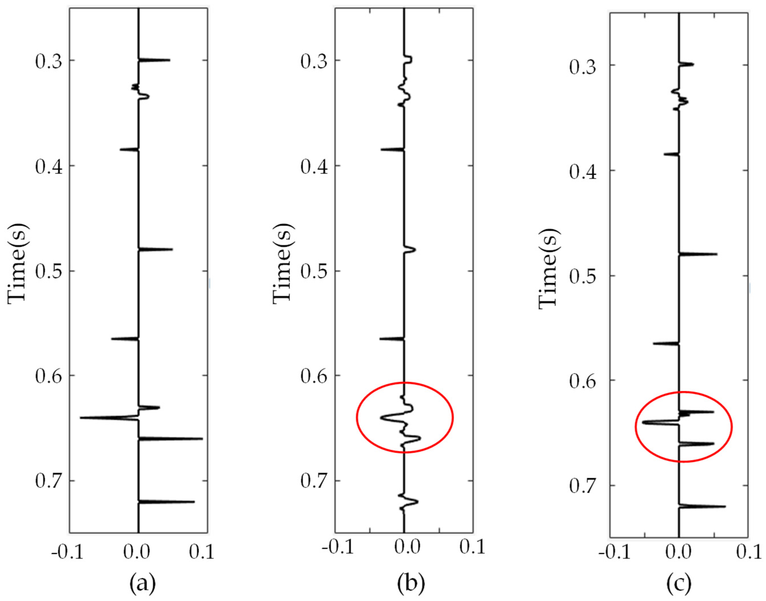
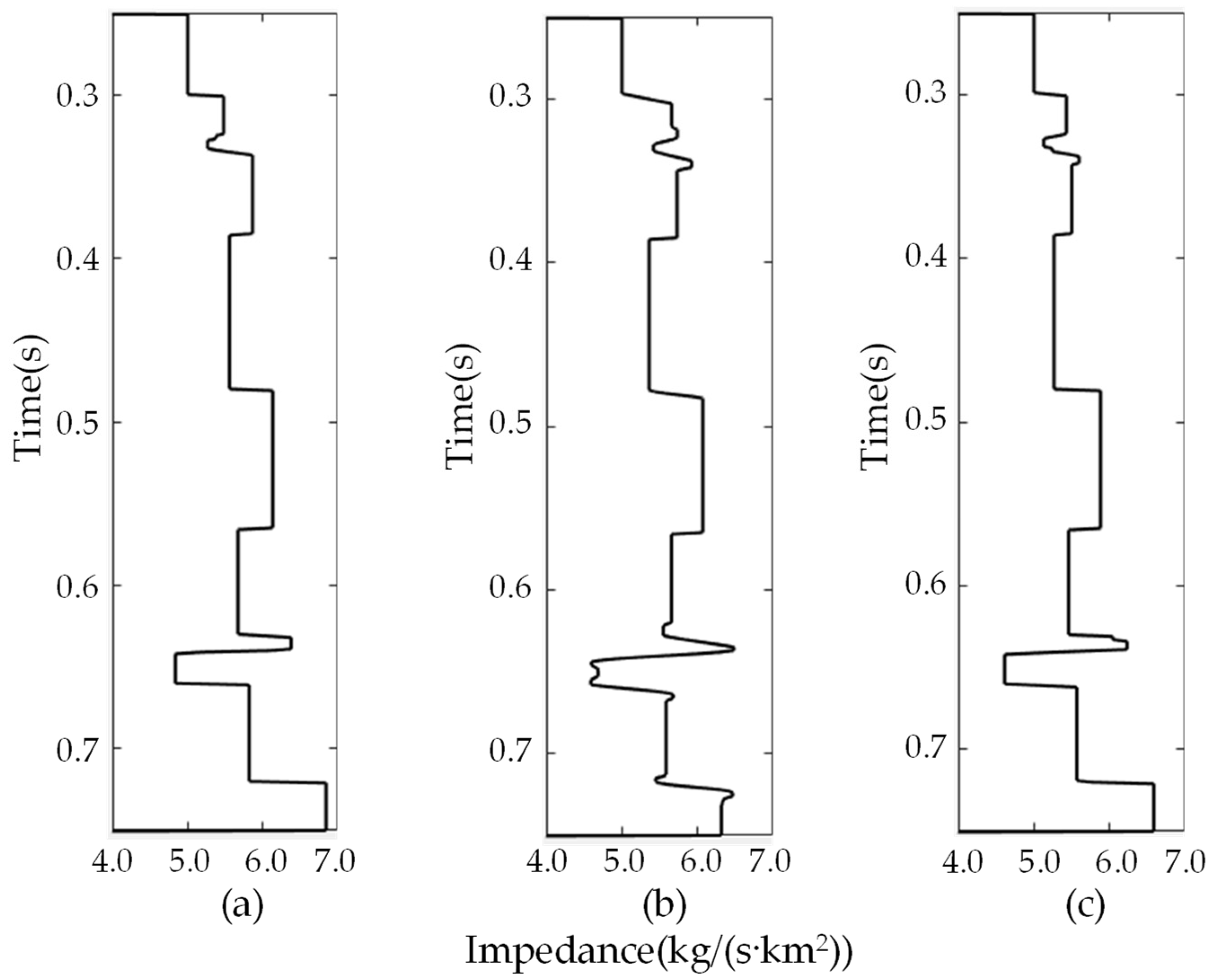
In order to further test the stability (i.e., noise resistance) of IHyTA compared to IHTA, 20% Gaussian random noise with zero mean was added to the synthetic seismic data. The noise-contaminated seismic data is shown in Figure 1c. Then, IHTA and IHyTA are applied to this noise-contaminated seismic data with the same regularization parameters and tolerance values. The initial solution and the a priori model are also the same as the above tests. The inverted reflectivity series from IHTA and IHyTA are plotted in the last two panels of Figure 4, respectively. The inverted impedance from IHTA and IHyTA are plotted in the last two panels of Figure 5, respectively. Figure 4 and Figure 5 show that the reflectivity series and impedance inverted by IHyTA from noise-contaminated seismic data with small ration of signal to noise (SNR) is more accurate, especially at some small reflectivity series (note at the position in ovals). Hence, IHyTA improves the noise resistance.

Figure 4. The true reflectivity series and inverted reflectivity series with synthetic seismic data in Figure 1c. (a) true; (b) IHTA; (c) IHyTA.

Figure 5. The true impedance and inverted impedance with synthetic seismic data in Figure 1c. (a) true; (b) IHTA; (c) IHyTA.

To assess the quality of the inverted reflectivity series produced by reflectivity series quantitatively, the relative errors (RE) and correlation coefficient (CC) are computed for the various inverted reflectivity series in comparison to the true reflectivity series. The RE are calculated by:

$$\mathrm{RE}={\displaystyle \frac{{‖\hat{r}-r‖}_2^2}{{‖r‖}_2^2}},$$

(21)

where r is the true reflectivity series, and $\hat{r}$ is the inverted reflectivity series. And the CC are calculated by the common formula in statistics.

The REs and CCs are detailed in Table 1 and Table 2. As indicated in Table 1 and Table 2, in the case of different noise case, the REs of the inverted reflectivity series produced by IHyTA are both lower than those of the inverted reflectivity series by IHTA, and the CCs of the inverted reflectivity series produced by IHyTA are both larger than those of the inverted reflectivity series by IHTA.

Table 1. The REs of inverted reflectivity series by different algorithms.

Inversion Method	RE (5% Random Noise)	RE (20% Random Noise)
IHyTA	0.0599	0.0829
IHTA	0.1025	0.1276

Table 2. The CCs of inverted reflectivity series by different algorithms.

Inversion Method	CC (5% Random Noise)	CC (20% Random Noise)
IHyTA	0.9551	0.8879
IHTA	0.8212	0.7553

In addition, we compare the computational times of IHTA, FIHTA, IHyTA, and OTA proposed by Zhao with the interior point method [20]. The computational times are recorded when they reach the maximum number of iteration. In this case, we set the maximum number of iteration equal to 500. The results are listed in Table 3. One can see that OTA costs the most computational time while FIHTA costs the least computational time. IHyTA costs a moderate amount of time. The reasons are that, in each iteration, OTA uses the interior point method to perform the optimal thresholding, which is time-consuming; on the other hand, IHTA and FIHTA just perform hard thresholding or inertial acceleration steps in each iteration [8]. Hence, the computation costs are lower compared to OTA and IHyTA.

Table 3. The computational times for synthetic seismic data tests by different algorithms.

Inversion Method	Times (ms)
IHyTA	311
IHTA	165
FIHTA	62
OTA	1788

3.2. Real Seismic Data Applications

Next, in order to evaluate the applicability of IHyTA on real seismic data, we use a real 3D seismic data volume from East China. The seismic data volume includes 101 Inlines from 545 to 645, and each Inline contains 61 Crosslines from 795 to 855. 3D seismic is recorded over an area in which data is sampled densely along a regular grid and the processed output is available in a volume. On land, 3D acquisition is done with a closely spaced grid of shot and receiver points spread over an area called a “swath”. Along the swath, receivers are placed on parallel lines and shot points are positioned on parallel lines (which are the so-called Crosslines) orthogonal to receiver lines (which are the so-called Inlines).

An interpolated impedance model is built by Kriging interpolation method with actual well logs in this work area under the constraint of seismic geologic horizon. After that, the 15 Hz low-pass filter is performed on the interpolation model to obtain a low-frequency model to serve as the a priori constraint and initial solution of IHyTA. Then, IHyTA is applied to the real seismic data volume.

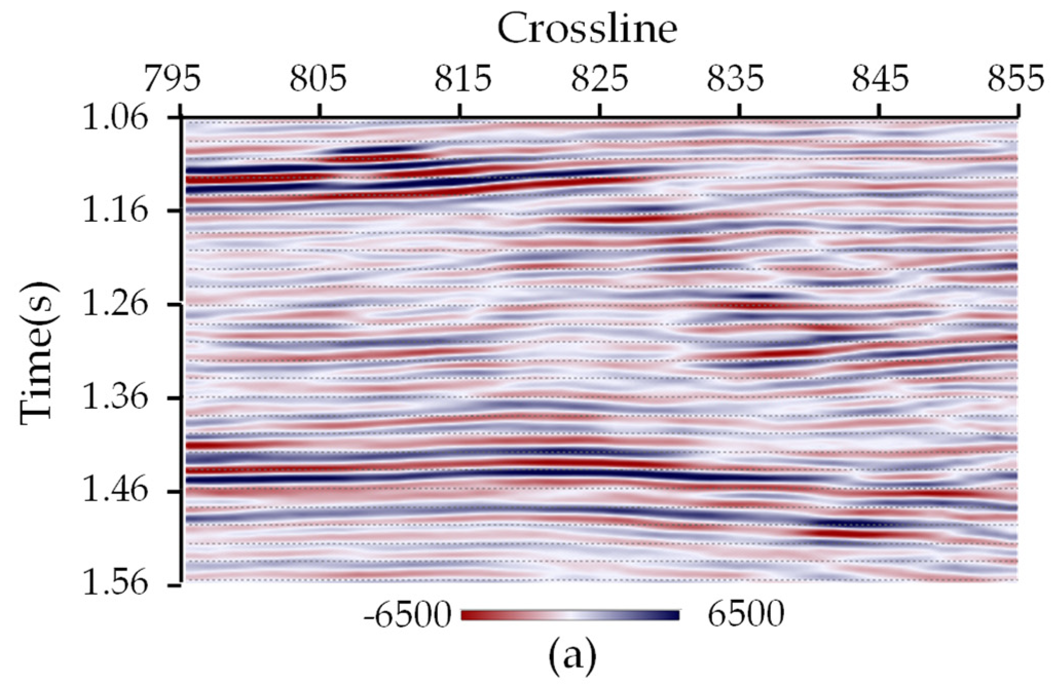
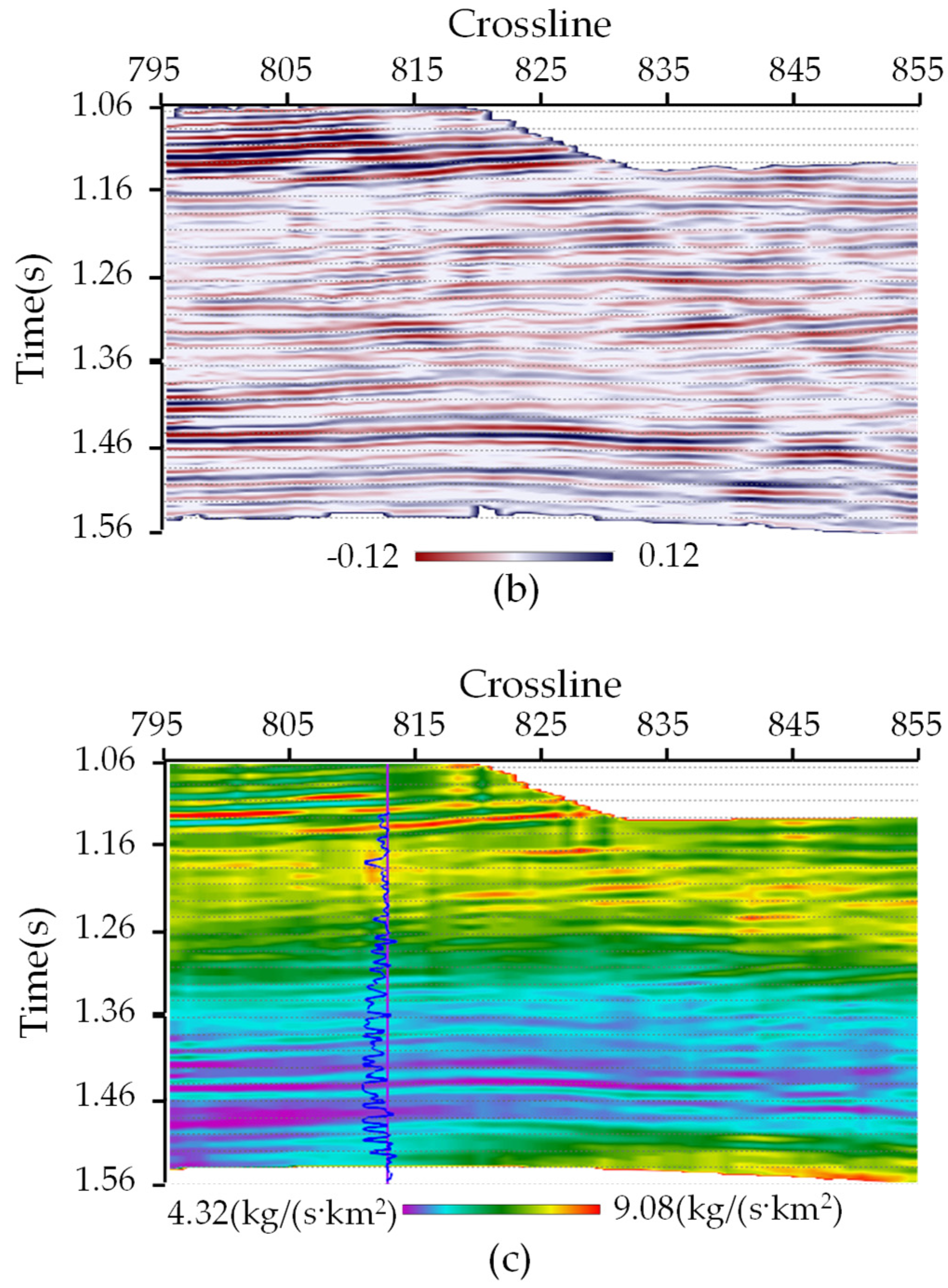
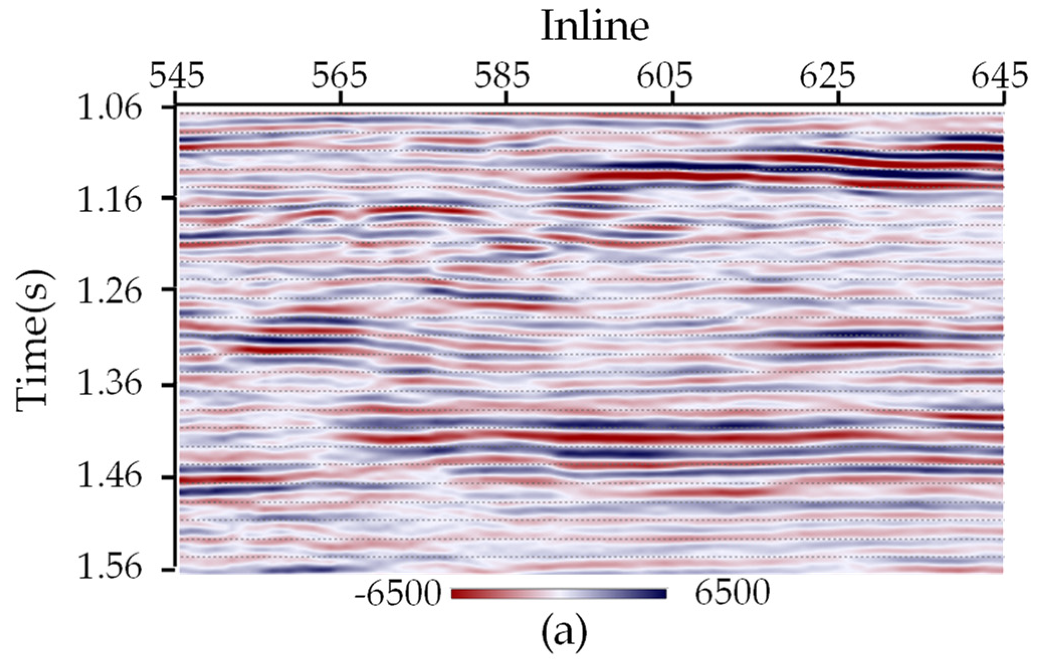
Figure 6a–c displays the real seismic data profile for Inline 598 and its corresponding inverted reflectivity series profiles and inverted impedance profiles in color, respectively. The vertical axe is the travel time of seismic wave, and the horizontal axe is the Crossline number at Inline 598. Furthermore, Figure 7a–c displays the real seismic data for Crossline 800 and its corresponding inverted reflectivity series profiles and inverted impedance profiles in color, respectively. The vertical axe is the travel time of seismic wave, and the horizontal axe is the Inline number at Crossline 800. It can be seen that the inverted reflectivity series matches well with the original seismic data and have good tectonic structure and lateral distribution of strata. The inverted impedance also matches well with the logging data. In the inverted impedance, the main stratigraphic boundaries are exact. The inversion results have “blocky behavior”, characterized by sparse constraints; that is, the contrast between the layers is obvious. The resolution of the inverted reflectance series is significantly higher than that of the original seismic data. Major stratigraphic boundaries are accurately delineated in the inverted impedance. The clear vertical and spatial variation features of estimated reflectivity series and impedance can be well-used in the further reservoir prediction and description. For example, the streaks shown in purple near 1.46 s in the Figure 6 and Figure 7 are the underground distribution of the impedance of a rock in a certain formation.

Figure 6. The real seismic data profile for Inline 598, and its corresponding inverted reflectivity series profiles and inverted impedance profiles. (a) real seismic data; (b) reflectivity series; (c) impedance.

Figure 7. The real seismic data for Crossline 800, and its corresponding inverted reflectivity series profiles and inverted impedance profiles. (a) real seismic data; (b) reflectivity series; (c) impedance.

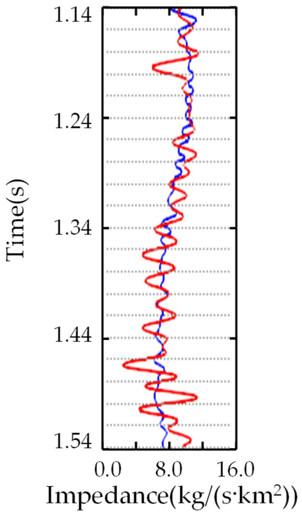
Figure 8 visually compares the inverted impedance of the well position with the real logging data, where the blue line represents the inverted impedance and the red line represents the logging data. The vertical axe is the travel time, and the horizontal axe is the value of impedance. It can be seen that the inverted impedance matches the real log data on the relative trend.

Figure 8. The single trace comparison between well log data and inverted impedance. The red curve is well log, the blue curve is inverted impedance.

4. Discussions

The basic idea of this paper is to solve the sparse-spike seismic inversion with L0-norm sparse regularization through the idea of ROTA. However, the interior point method in ROTA is too time-consuming to deal with massive real seismic data.

In the solution process, due to the particularity of the sparse constraints in the convex relaxation model of ROTA, we formulate it as a L1-norm problem when dealt with the location of non-zero elements and use a MISTA to solve it. Combining IHTA and ISTA, it forms the proposed IHyTA. The feasibility, convergence, and convergence rate of IHyTA have not been analyzed. But we use synthetic data and real data application to test its feasibility and noise resistance. Using the theoretical analysis on convergence and convergence rate of IHyTA, one can follow Zhao’s work [20]. We hope that readers interested in this work will do this work. It is not described specifically here. We cannot do this work due to the lack of relevant mathematical knowledge for the theoretical analysis of algorithms. We, the authors, are engaged in the practical application of mathematics in geophysics.

In addition, in the practical application of seismic inversion, computational efficiency is a key factor to be considered. There is not only the external loop like IHTA or ROTA, but also the inner loop of MISTA, which may lead to more iterations. When dealing with massive real seismic data, there is a compromise between the computation cost and the convergence rata. A faster version of IHyTA can be a topic in the future. Nesterov’s accelerated method [26] or Momentum acceleration method [27] may be two good choices.

To choose the appropriate regularization parameters, we use quality control to determine these regularization parameters in this paper. It needs available actual well logs. In quality control, we think the actual well logs are the ”answer” to the inversion of near-well seismic traces. The actual well logs represent the actual geological setting of underground formations. The best value of regularization parameters is determined by doing quality control at well locations. That is, adjust the value of the regularization parameters, obtain the inversion result from the near well seismic traces for each set of regularization parameters, and choose the one whose inversion result has the best match with the well log. Then, the chosen regularization parameters are adopted when we perform inversion for other seismic traces.

In addition, regularization is a common technique used in machine learning and deep learning, which aims to improve the generalization ability of the model by introducing penalty terms and limiting its complexity. Among these, L1 regularization and L2 regularization are the most common regularization methods. The problem in this paper is similar to machine learning models, based on which, in future work, we can combine the sparse-spike seismic inversion with machine learning models and deep learning methods. In the inversion process, try to apply machine learning methods, such as EM algorithm, Monte Carlo method, Markov Chain, neural network learning, etc.

5. Conclusions

Noise resistance is a key factor to be considered in the practical application of seismic inversion. To this end, we propose IHyTA to solve sparse-spike seismic inversion. The main contributions of this algorithm are that it inherits the advantages of ROTA, which can avoid residue’s oscillation and loss of large amounts of information from small elements and combines IHTA and ISTA to make the inversion results more stable to better suppress the noise, and protects small reflectivity series compared to IHTA. We use a synthetic seismic data trace and a real seismic data volume to test the performance of IHyTA. Compared with IHTA, the inversion results of IHyTA are more accurate with the same SNR. In the case of different noise case, the REs of the inverted reflectivity series produced by IHyTA are both lower than those of the inverted reflectivity series by IHTA, and the CCs of the inverted reflectivity series produced by IHyTA are both larger than those of the inverted reflectivity series by IHTA. Hence, we can conclude that the proposed algorithm significantly improves the accuracy of inversion results and enhances the noise resistance. It provides a new effective alternative to solving the sparse-spike seismic inversion.

References

- Wu, Q.; Huang, W.; Qiao, B. Integrated seismic prediction techniques research on sandstone-type uranium deposit: A case study of uranium deposit in Qiharigetu depression. Prog. Geophys. 2018, 33, 2002–2014. [Google Scholar]
- Zhang, F.; Dai, R.; Liu, H. Seismic inversion based on L1-norm misfit function and total variation regularization. J. Appl. Geophys. 2014, 109, 111–118. [Google Scholar] [CrossRef]
- Wang, Y. Seismic Inversion: Theory and Applications; Wiley-Blackwell: Malden, MA, USA, 2017; pp. 68–83. [Google Scholar]
- Liu, D.; Niu, W.; Wang, X.; Sacchi, M.D.; Chen, W.; Wang, C. Improving vertical resolution of vintage seismic data by a weakly supervised method based on cycle generative adversarial network. Geophysics 2023, 88, V445–V458. [Google Scholar] [CrossRef]
- Renaut, R.A.; Hnetynkova, I.; Mead, J. Regularization parameter estimation for large-scale Tikhonov regularization using a priori information. Comput. Stat. Data Anal. 2010, 54, 3430–3445. [Google Scholar] [CrossRef][Green Version]
- Tarantola, A. Inverse Problem Theory and Methods for Model Parameter Estimation; SIAM: Philadelphia, PA, USA, 2005; pp. 101–158. [Google Scholar]
- Bouchot, J.L. A generalized class of hard thresholding algorithms for sparse signal recovery. In Approximation Theory XIV: San Antonio 2013, Proceedings of the 14th International Conference on Approximation Theory, San Antonio, TX, USA, 7–10 April 2013; Springer Proceedings in Mathematics & Statistics; Fasshauer, G., Schumaker, L., Eds.; Springer: Berlin/Heidelberg, Germany, 2013; Volume 83, pp. 45–63. [Google Scholar]
- Li, G.; Yang, J.; Yang, W.; Wang, Y.; Wang, W.; Liu, L. 2D Normalized Iterative Hard Thresholding Algorithm for Fast Compressive Radar Imaging. Remote Sens. 2017, 9, 619. [Google Scholar] [CrossRef]
- Moosaei, H.; Hladik, M. Sparse solution of least-squares twin multi-class support vector machine using l0 and lp-norm for classification and feature selection. Neural Netw. 2023, 166, 471–486. [Google Scholar] [CrossRef] [PubMed]
- Bi, H.; Li, Y.; Zhu, D.; Bi, G.; Zhang, B.; Hong, W.; Wu, Y. An improved iterative thresholding algorithm for L1-norm regularization based sparse SAR imaging. Sci. China 2020, 63, 330–339. [Google Scholar] [CrossRef]
- Candes, E.J.; Wakin, M.B.; Boyd, S.P. Enhancing sparsity by reweighted ℓ1 minimization. J. Fourier Anal. Appl. 2008, 14, 877–905. [Google Scholar] [CrossRef]
- Alemie, W.; Sacchi, M.D. High-resolution three-term AVO inversion by means of a Trivariate Cauchy probability distribution. Geophysics 2011, 76, 43–55. [Google Scholar] [CrossRef]
- Dai, R.; Zhang, F.; Liu, H. Seismic inversion based on proximal objective function optimization algorithm. Geophysics 2016, 81, 237–246. [Google Scholar] [CrossRef]
- Sacchi, M.D. Reweighting strategies in seismic deconvolution. Geophys. J. Int. 1997, 129, 651–656. [Google Scholar] [CrossRef]
- Zhang, F.; Dai, R. Nonlinear inversion of pre-stack seismic data using variable metric method. J. Appl. Geophys. 2016, 129, 111–125. [Google Scholar] [CrossRef]
- Aravkin, A.; Friedlander, M.P.; Herrmann, F.J.; Leeuwen, T.V. Robust inversion, dimensionality reduction, and randomized sampling. Math. Program. 2012, 134, 101–125. [Google Scholar] [CrossRef]
- Li, C.; Zhang, F. Amplitude-versus-angle inversion based on the L1-norm-based likelihood function and the total variation regularization constraint. Geophysics 2017, 82, R173–R182. [Google Scholar] [CrossRef]
- Dai, R.; Yang, J. An alternative method based on region fusion to solve L0-norm constrained sparse seismic inversion. Explor. Geophys. 2021, 52, 624–632. [Google Scholar] [CrossRef]
- Simon, F. Hard thresholding pursuit: An algorithm for compressive sensing. SIAM J. Numer. Anal. 2011, 49, 2543–2563. [Google Scholar]
- Zhao, Y. Optimal k-thresholding algorithms for sparse optimization problems. SIAM J. Optim. 2020, 30, 31–55. [Google Scholar] [CrossRef]
- Cipolla, S.; Gondzio, J.; Zanetti, F.; Slowinski, R.; Artalejo, J.; Billaut, J.; Dyson, R.; Peccati, L. A regularized interior point method for sparse optimal transport on graphs. Eur. J. Oper. Res. 2024, 319, 413–426. [Google Scholar] [CrossRef]
- Sun, J.; Du, S. An effective smoothing Newton projection algorithm for finding sparse solutions to NP-hard tensor complementarity problems. J. Comput. Appl. Math. 2024, 451, 116074. [Google Scholar] [CrossRef]
- Koutrouvelis, A.I.; Hendriks, R.C.; Heusdens, R.; Jensen, J.R. A Convex Approximation of the Relaxed Binaural Beamforming Optimization Problem. IEEE/ACM Trans. Audio Speech Lang. Process. 2019, 27, 321–331. [Google Scholar] [CrossRef]
- Cao, D.; Yin, X.; Zhang, F.; Kong, Q. A study on the method of joint inversion of multiscale seismic data. Chin. J. Geophys. 2009, 52, 1059–1067. (In Chinese) [Google Scholar]
- Wang, Y. Time-Frequency Analysis of Seismic Signals; Wiley: Hoboken, NJ, USA, 2023. [Google Scholar]
- Nesterov, Y. Basis Course. In Introductory Lectures on Convex Optimization; Springer: New York, NY, USA, 2003. [Google Scholar]
- Ning, Q. On the momentum term in gradient descent learning algorithms. Neural Netw. 1999, 12, 145–151. [Google Scholar]
Disclaimer/Publisher’s Note: The statements, opinions and data contained in all publications are solely those of the individual author(s) and contributor(s) and not of MDPI and/or the editor(s). MDPI and/or the editor(s) disclaim responsibility for any injury to people or property resulting from any ideas, methods, instructions or products referred to in the content. |
© 2024 by the authors. Licensee MDPI, Basel, Switzerland. This article is an open access article distributed under the terms and conditions of the Creative Commons Attribution (CC BY) license (https://creativecommons.org/licenses/by/4.0/).