Article

Analyzing Russia–Ukraine War Patterns Based on Lanchester Model Using SINDy Algorithm

Department of Mathematics, Keimyung University, Daegu 42601, Republic of Korea
*
Author to whom correspondence should be addressed.
Mathematics 2024, 12(6), 851; https://doi.org/10.3390/math12060851
Submission received: 25 January 2024 / Revised: 4 March 2024 / Accepted: 11 March 2024 / Published: 14 March 2024
(This article belongs to the Section Dynamical Systems)

Abstract

:
In this paper, we present an effective method for analyzing patterns in the Russia–Ukraine war based on the Lanchester model. Due to the limited availability of information on combat powers of engaging forces, we utilize the loss of armored equipment as the primary data source. To capture the intricate dynamics of modern warfare, we partition the combat loss data into disjoint subsets by examining their geometric properties. Separate systems of ordinary differential equations for these subsets are then identified using the Sparse Identification of Nonlinear Dynamics (SINDy) algorithm under a generalized formulation of the historical Lanchester model. We provide simulations of our method to demonstrate its effectiveness and performance in analyzing contemporary warfare dynamics.

1. Introduction

Throughout history, warfare has evolved from small-scale tribal conflicts to complex battles involving numerous stakeholders utilizing advanced technology and intricate strategies. Although warfare has undergone various complex evolutions, the fundamental need to predict outcomes, interpret the dynamics of military confrontations, and understand the nature of essence of war remains unchanged. This persistent need has led to the creation of numerous mathematical models to capture the dynamics of combat, most notably the Lanchester model [1]. The Lanchester Attrition Model employs differential equations to predict the outcomes of military engagements by taking into account the numerical strength and combat efficiency of the forces involved. This model has played a pivotal role in the analysis of military confrontations for several decades, and many mathematical methods have been developed for its application in diverse scenarios.
Morse and Kimball proposed a linear Lanchester model focusing on aimed fire and small skirmishes [2]. Weiss explored the model in the context of the American Civil War [3], while Peterson suggested a tensorial generalization of the early Lanchester-type equations and examined the feasibility of the exponential Lanchester model for armored combat [4]. Dietchman [5] and Schaffer [6] introduced variants for irregular warfare. In addition, Hartley and Helmbold used data from the Inchon Landing during the Korean War—a confrontation between the U.S. 1st Marine Division and the North Korean Army—to develop an exponential Lanchester model [7]. In [8], recent advances in Lanchester modeling, focusing on modern conflicts and capturing the role of targeting information in irregular warfare such as insurgencies, were reviewed, and models that captured the multi-party situation of conflicts were presented in [8,9]. In addition to the traditional Lanchester model, which uses ordinary differential equations, partial differential equation-type models that incorporate spatial information have been introduced in [10,11,12]. They have also recently been used in a variety of fields such as combat in nonhuman animals [13], human evolution [14], market share competition [15], and video games [16].
The Russia–Ukraine war, which began on 24 February 2022, epitomizes contemporary warfare. Characterized by geopolitical tensions, this war manifests a mix of traditional military tactics, guerrilla warfare, cyberattacks, and cutting-edge technology. Recent developments in artificial intelligence and networking made it possible to aggregate and process data from various battlefronts in real-time. In this paper, our objective is to apply the Lanchester model to this contemporary conflict using extensive combat force loss data from both nations to find ways to improve or adapt the model. In particular, to prevent the fidelity deterioration of a developed model to the data, we partition the time-series data based on their geometric properties into disjoint subsets and model a system for each subset rather than identifying a single system for the extensive dataset.
Throughout history, various forms of conflict have continuously emerged, directly and indirectly affecting not only the parties involved but also a wide range of people. This research was motivated by the desire to gain deeper insights into the dynamics of modern warfare and to bridge the gap between historical combat models and the complexity of modern warfare. To achieve this goal, this paper applies the Sparse Identification of Nonlinear Dynamics (SINDy) [17] algorithm to armor-centric combat loss data from the ongoing war between Russia and Ukraine. SINDy is a data-driven algorithm for discovering the governing equations of nonlinear dynamical systems. The algorithm constructs a library of potential terms that may appear in the equations and then uses sparse regressions to identify the subset of terms that are actually relevant, approximating the data’s governing equations. SINDy is especially useful for dynamical systems that are too complex for analytical modeling or where noisy data are available. One of the primary benefits of SINDy is its ability to directly identify the system’s governing equations from data, without any prior knowledge of the system’s dynamics. This enables the discovery of governing equations for complex systems that are not amenable to traditional modeling approaches. Moreover, SINDy can be used to reduce the complexity of a model by identifying a subset of terms essential for capturing the dynamics of the system, allowing for more efficient simulation and analysis. Numerous applications and variants of the SINDy algorithm in modeling dynamical systems can be observed, encompassing recent works such as [18,19,20,21,22,23,24]. The Lanchester model is a nonlinear dynamical system, and for some models, the dynamical equations are difficult to solve analytically. In this paper, we utilize SINDy to identify the governing equations of the Lanchester model from attrition data of combat equipment. Subsequently, we simulate and analyze the dynamics of the system.
The paper is structured to first provide a theoretical review of the simple Lanchester model, setting the foundation for our more complex investigations in Section 2. We then describe the armor-centric loss data from the Russia–Ukraine war, detailing why this particular set of data provides a unique opportunity for analysis in Section 3. After introducing the SINDy algorithm in Section 4, we present our method for identifying systems that fit the given data based on the Lanchester model in Section 5. The simulation and analysis of the resulting models, along with a discussion of the implications of our findings, will be presented in Section 6. Finally, in Section 7, we present the conclusions of our study.

2. Lanchester Model

The Lanchester model describes the time-variant changes in the combat power of two engaging forces. It employs two elements: the combat power and combat efficiency, expressed in the form of differential equations. Generally, equations can be represented assuming two scenarios. One is where the combat between forces is centered around aimed fire, where the differential equations are as follows:
x = α y , y = β x ,
where x = x ( t ) and y = y ( t ) represent the total combat power of the two factions, x and y, at time t > 0 . The other scenario is characterized by primarily unaimed fire. In situations of combat where both parties engage in area fire, such as artillery barrages, the general locations of the opposing forces are known. However, the precise positions and outcomes of their fire are uncertain, making concentrated fire through aiming impossible. In situations where the opposing side engages in area fire, the potential loss of combat power increases with one’s own combat power. Therefore, the rate of loss of one’s own forces is not only proportional to the combat power of the opponent but also to one’s own combat power. The differential equations for this scenario are as follows.
x = α x y , y = β x y .
The analysis of this system is well known under Lanchester’s square law and linear law. Formulated as a theorem, these laws can be articulated as follows.
Theorem 1
(Lanchester’s Square and Linear Law). The solutions to Equations (1) and (2), respectively, satisfy the following state equations.
α ( y 0 2 y 2 ) = β ( x 0 2 x 2 ) ( Square Law ) α ( y 0 y ) = β ( x 0 x ) ( Linear Law )
where x 0 = x ( 0 ) and y 0 = y ( 0 ) .
The above theorem can be easily proven by separating the variables after dividing each equation and then integrating both sides. The solutions to Equations (1) and (2) are well known, and their asymptotic behaviors are easily understood. For explicit forms of solutions and a detailed analysis of their behaviors, readers may refer to [9]. In scenario Equation (2), where the change in combat power of both sides is proportional to the size of their forces, an alternative expression can be used. Instead of assuming that the change in force size is proportional to the product of the sizes of both forces, it can be assumed that the change in force size is proportional to the size of each force individually. Additionally, by incorporating additional factors beyond the force size, the following differential equation model can be constructed.
x = a 1 + b 1 x + c 1 y , y = a 2 + b 2 x + c 2 y .
In the classical model, the coefficients b 1 and c 2 are considered the non-combat attrition rates for each side due to accidents, diseases, desertions, and other factors. Meanwhile, a 1 and a 2 are defined as the reinforcements of combat power for each force, respectively. In the classical model, all coefficients are stipulated to be negative. However, modern warfare is highly complex and influenced by various internal and external factors. Therefore, the restriction on the sign of the coefficients is unnecessary.
Reducing systems of ODEs to simple forms of state equations, as presented in Theorem 1, can be challenging. However, the coefficients’ magnitude and sign can help explain the specific conflict’s complex nature. In the above equation, a 1 and a 2 represent the influence of external factors on the change in combat power, while b 1 , b 2 , c 1 , and c 2 can be considered as the rate of change due to the size of each respective combat power. The solution to the equation above can be expressed in closed form as follows.
Lemma 1.
The solutions of (3) are as follows:
x ( t ) = k 1 ( λ 2 b 1 ) e λ 1 t + k 2 ( λ 1 b 1 ) e λ 2 t + a 1 c 2 b 1 c 1 b 1 b 2 + a 1 y ( t ) = k 1 a 2 e λ 1 t + k 2 e λ 2 t + a 2 c 1 b 1 c 2 b 1 b 2 + a 1
where λ 1 , 2 = b 1 + b 2 ± ( b 1 + b 2 ) 2 4 ( b 1 b 2 + a 1 ) 2 and k 1 , k 2 are some constants.
Creating a scenario that accurately represents the complex nature of warfare is a challenging task. The changes in combat power of the forces are generally presumed to be proportional to their size, but the exact nature of this proportionality is difficult to ascertain. To represent the system in a more general form, the following system of equations may be used.
x = a 1 + b 1 x + c 1 y + d 1 x 2 + e 1 x y + f 1 y 2 + , y = a 2 + b 2 x + c 2 y + d 2 x 2 + e 2 x y + f 2 y 2 + .
This paper aims to estimate equations that represent the nature of warfare, focusing on recent armored warfare data from Russia and Ukraine, using the SINDy algorithm recalled in the following section. However, information about the combat power of each nation is classified. In particular, data on the combat power at the beginning of hostilities is a national secret and not easily accessible. Therefore, we will consider the loss of armored equipment reported through the media as a loss of combat power and adjust the equations accordingly based on these data.
Remark 1.
If x ¯ ( t ) and y ¯ ( t ) are defined as the cumulative losses of combat power up to time t for each side, then the combat power of the two factions can be expressed as
x ( t ) = x ( 0 ) x ¯ ( t ) , y ( t ) = y ( 0 ) y ¯ ( t ) .
Substituting the above expression into the equation concerning combat power yields an equation for the combat power loss. For instance, substituting expression (5) into Equation (3) allows for the derivation of a system concerning the cumulative combat power losses of both forces as follows:
x ¯ = ( a 1 + b 1 x 0 + c 1 y 0 ) + b 1 x ¯ + c 1 y ¯ , y ¯ = ( a 2 + b 2 x 0 + c 2 y 0 ) + b 2 x ¯ + c 2 y ¯ ,
where x 0 = x ( 0 ) and y 0 = y ( 0 ) .

3. Russia–Ukraine Data

In warfare, the loss of equipment by the warring parties is a highly confidential matter, making it challenging to acquire accurate data on the combat losses of both sides. However, the recent advancements in artificial intelligence technology have made it possible to collect specific data such as specific types of equipment, country of manufacture, and year of production for the equipment lost in combat by both sides. This is achieved by gathering photos and videos of the lost equipment. Particularly, ref. [25] is currently providing daily updates on the combat losses of both countries in the ongoing Russia–Ukraine war. Ref. [25] utilizes such photographic and video evidence to update a list of destroyed vehicles and equipment daily. Through this site, we have acquired data on the combat equipment losses of Russia and Ukraine during the period from 24 February 2022 to 25 September 2023. The data obtained from [25] is based on photographic and video evidence, indicating that the actual combat losses may be much greater than recorded. Additionally, while ref. [25] categorizes the lost combat equipment into destroyed, abandoned, and captured, we have not distinguished between these as they are all considered combat incapacitated. In this paper, we have focused on armored equipment and used weights for each piece of equipment similar to those used in a previous study [26] on fitting Lanchester model for armored warfare. Ref. [26] applied the Lanchester model to fit data from the Battle of Kursk. The Battle of Kursk was a battle that focused on armor and was fought in a region similar to that of the Russia–Ukraine War, although at a different time. In modern ground warfare, tanks and artillery are both crucial pieces of equipment, each with its own advantages and disadvantages. The importance of tanks and artillery varies depending on the situation. However, since this paper focuses on combat losses, considering the average price of both types of equipment, weights in [26] are used. Table 1 shows the types of combat loss equipment used in this paper and the weight for each type.

4. SINDy Algorithm

In this section, we will provide a brief review of the SINDy algorithm [17], which is employed for model discovery and system identification. In the context of a dynamical system
x ( t ) = f ( x ( t ) )
for x ( t ) : = ( x 1 ( t ) , x 2 ( t ) , , x J ( t ) ) , x ( t ) : = ( x 1 ( t ) , x 2 ( t ) , , x J ( t ) ) , and f : = ( f 1 , f 2 , , f J ) with f j : R J R , the algorithm aims to determine an efficient representation of f concerning basis functions that best describe the dynamics of measurement data { x ( t n ) : n = 1 , , N } for N J . A library of polynomials, trigonometric functions, or other relevant mathematical expressions may be used to represent f . We can numerically approximate the derivative values, { x ( t n ) } , from the given data set, { x ( t n ) } , in cases where the derivative values are not available. Let { φ : R J R : = 1 , , L } for L N be a candidate library. We then consider a sparse regression problem of the form
X = Φ A ,
where
X : = [ x ( t n ) : n = 1 , , N ] R N × J , Φ : = [ φ ( x ( t n ) ) : n = 1 , , N , = 1 , , L ] R N × L , A : = [ α , j : = 1 , , L , j = 1 , , J ] R L × J .
The sparse solution A to this overdetermined system is obtained using the Sequential Thresholded Least-Squares (STLS) method, which can be formulated as
min A 1 2 X Φ A 2 + η R ( A ) ,
where η is the sparsity parameter, and R indicates the regularization function. See [17,27] for details.

5. Proposed Method

The objective of this section is to introduce an effective method for deriving a system of ordinary differential equations that captures the dynamics of Russia–Ukraine warfare. Due to the unavailability of initial combat strengths for both Russian and Ukrainian forces, we model the dynamics using the cumulative losses measured as in Section 3. This approach can be considered an alternative application of the Lanchester model, as discussed in Remark 1. On the other hand, since the duration of the warfare is long (579 days) enough to exhibit diverse patterns resulting from changes in tactics or strategies during battle, we opt to identify separate systems over subintervals of time to better capture the evolving character of the data, rather than using a single system for the entire period.

5.1. Partition of Data

To implement the above discussion, we partition the entire set of measurement data into disjoint subsets by examining the geometric properties of the data, specifically focusing on the sign changes in their second-order derivatives. For this purpose, we initially create a smooth approximation of the data using the Moving Least Squares (MLS) method [28]. The reason for choosing the MLS method is that when averaging the data using this method, we can control the number of contributing data points, the distribution of weights, and the accuracy of approximation based on the data properties. To be specific, let { f ( t n ) : n = 1 , 2 , , N } be the data values in a neighborhood of an evaluation point t. The approximation A f of the value f at location t is given by the expression
A f ( t ) = n = 1 N a n ( t ) f ( t n ) ,
where the coefficients { a n } are determined by solving the minimization problem
min { a n } n = 1 N a n ( t ) 2 θ ( t n , t ) subject to n = 1 N a n ( t ) p ( t n ) = p ( t ) , = 0 , 1 .
Here, θ is a penalty function depending on the distance between t n and t, e.g., θ ( t , s ) = exp ( ( t s ) 2 / h 2 ) , and p ( · ) : = ( · t ) . The problem (7) can be solved by applying the Lagrange multipliers method. Using the matrix notation, the solution a : = [ a n ( t ) : n = 1 , , N ] T R N × 1 can be represented as
a = D 1 P ( P T D 1 P ) 1 p ,
where
D : = 2 diag ( θ ( t 1 , t ) , , θ ( t N , t ) ) R N × N , P : = [ p 0 ( t n ) p 1 ( t n ) : n = 1 , , N ] R N × 2 , p : = [ p 0 ( t ) p 1 ( t ) ] T R 2 × 1 .
Next, we calculate the second-order finite differences, 2 A f , from the approximated data A f , and apply the MLS method to the differences if smoothing is needed to facilitate our investigation into the shape of the data. The resulting finite differences are denoted by ˜ 2 f . Subsequently, we identify points where the sign of ˜ 2 f changes. Based on these locations, we partition the entire set T of sampling times into K disjoint subsets T k for k = 1 , 2 , , K .

5.2. Identification of System

Let x = x ( t ) and y = y ( t ) be the state variables representing the cumulative losses of Russian and Ukrainian combat forces at time t, respectively. For each subset T k obtained by applying the partitioning method from the previous subsection, we consider a system of the form
x ( t ) = f 1 ( x ( t ) , y ( t ) ) , y ( t ) = f 2 ( x ( t ) , y ( t ) ) ,
where functions f 1 and f 2 represent the dynamics constraints of the data x ( T k ) and y ( T k ) . In this paper, f 1 and f 2 are determined based on the generalized Lanchester model in (4). Specifically, we employ the SINDy algorithm described in Section 4 to identify a sparse set of coefficients using the library of polynomials of degree up to 2,
{ x p y q : 0 p + q 2 } .
Subsequently, for the resulting system, we conduct a phase plane analysis based on qualitative theory, as presented in [29]. We investigate the battle performance in terms of the ratio x / y , revealing patterns in Russia–Ukraine warfare. Refer to [30] for details on the ratio.

6. Simulations

In this section, we showcase the simulation results of the proposed method detailed in Section 5. We subdivide the complete dataset of Russia–Ukraine warfare, as obtained in Section 3, into six disjoint subsets using the method introduced in Section 5.1. We then identify a system representing the dynamics of warfare over each time interval by applying the SINDy algorithm discussed in Section 5.2.

6.1. Partitioned Times

Denoting by T : = Z [ 0 , 578 ] the set of sampling times during the entire period of the data, we applied the MLS approximation in (6) with a parameter setting of h = 30 to obtain the smoothed data A x ( T ) and A y ( T ) , along with their smoothed second-order finite differences ˜ 2 x ( T ) and ˜ 2 y ( T ) . For the MLS evaluation at each time t T , we used the data in the closest 61-point neighborhood of t (i.e., N = 61 ). Figure 1a–c illustrate the original data, their smoothed versions, and the finite differences, respectively. We located the points in T where the signs of ˜ 2 x ( T ) and ˜ 2 y ( T ) change. The union of these locations constitutes the candidates for the end points of each subinterval. The final locations for the partition were determined by taking the average of two points whose distance are smaller than 60. We obtained six disjoint subsets T k T for k = 1 , 2 , , 6 as
T 1 = { 0 , , 126 } , T 2 = { 127 , , 225 } , T 3 = { 226 , , 336 } , T 4 = { 337 , , 420 } , T 5 = { 421 , , 510 } , T 6 = { 511 , , 578 } .
The resulting partition is visualized in Figure 1c,d as dotted lines. If the character of data changes over time, unlike the scenario where the data are governed by a single system of equations throughout the entire time period, then the outcome of the system identification through a data-driven method, such as the SINDy algorithm, will depend on the choice of partition. The objective of the above approach is to find a suitable partition capturing the change in character by investigating the local properties of data.

6.2. Identified Systems

To identify systems of the form (8) capturing combat dynamics, we applied the SINDy algorithm to the data x ( T k ) and y ( T k ) for each subset T k in (10). For this, we used the polynomial library in (9) and applied the STLS method with a threshold of 5 × 10 4 . This results in a first-order linear system of the form
x = a 1 + b 1 x + c 1 y , y = a 2 + b 2 x + c 2 y ,
where the coefficients of the second-degree terms vanish. The solutions to this system reveal the characteristic of the warfare during the corresponding period. For a more informative analysis, we conduct a phase plane analysis for the system based on qualitative theory, as presented in [29]. Denoting
A : = b 1 c 1 b 2 c 2 ,
the solution to the system (11) can be characterized by the eigenvalues of the matrix A. To this end, we denote the characteristic equation of A by
λ 2 τ λ + δ = 0
for τ : = tr ( A ) and δ : = det ( A ) , and its discriminant by γ : = τ 2 4 δ . Moreover, we investigate the ratio x / y of loss rates, which assesses the battle performance in each period. Eventually, from the identified system over each time interval T k , we want to compute the quantities τ , δ , γ , and also x / y as a function of time. Our analysis results on the systems identified from the data x ( T k ) and y ( T k ) for T k , k = 1 , 2 , , 6 in (10) are presented as follows.
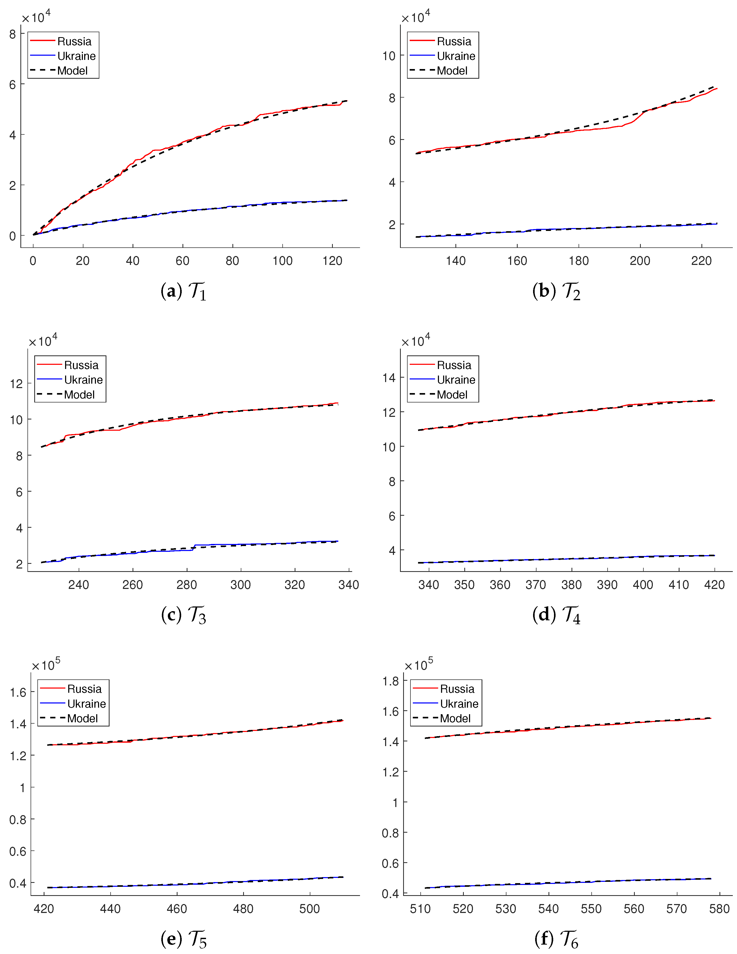
  • System over T 1 . From the data x ( T 1 ) and y ( T 1 ) with the initial values x ( 0 ) = 127 and y ( 0 ) = 178 , we obtained the coefficients of the system (11) as
a 1 = 8.8548 × 10 2 , b 1 = 4.0035 × 10 3 , c 1 = 6.7647 × 10 2 , a 2 = 2.2672 × 10 2 , b 2 = 1.0672 × 10 3 , c 2 = 1.7409 × 10 2 .
The solution to the system with these coefficients is illustrated in Figure 2a. To categorize the solution behavior, we compute τ , δ , and γ as defined in (12):
τ = 1.3405 × 10 2 , δ = 2.4958 × 10 6 , γ = 1.6972 × 10 4 .
According to the classification scheme in [29] Chapter 4.8, the solutions travel toward the equilibrium as time goes toward infinity. This implies that the dynamics of military confrontations approach a steady state as long as there is no change in strategy. The nature of warfare is further revealed by the exchange rate x / y [30]. As seen in Figure 3a, the exchange rate stays around 4; although, it is slightly decreasing. It indicates that the Russian force was losing its strength four times faster than Ukraine during this period.
  • System over T 2 . For the measurements x ( T 2 ) and y ( T 2 ) with the initial values x ( 127 ) = 53,307 and y ( 127 ) = 13,835, the coefficients were determined as
a 1 = 4.8645 × 10 2 , b 1 = 1.9494 × 10 2 , c 1 = 2.7033 × 10 2 , a 2 = 1.8309 × 10 2 , b 2 = 1.1743 × 10 3 , c 2 = 1.1203 × 10 2 .
The graph of the solution to the corresponding system is presented in Figure 2b. In this case, we have the quantities
τ = 8.2915 × 10 3 , δ = 1.8665 × 10 4 , γ = 8.1535 × 10 4 ,
from which the origin of the system is classified as a saddle point, meaning that the solutions travel away from the origin. This indicates that the combat effectiveness was one-sided in this time interval, a characteristic that can be precisely assessed by the ratio x / y . The ratio, depicted in Figure 3b, rapidly increases, implying that the battle performance of the Ukraine force was superior to its counterpart during this period.
  • System over T 3 . The losses x ( T 3 ) and y ( T 3 ) with the initial observations x ( 226 ) = 84,524 and y ( 226 ) = 20,525 were fitted by the system (11) with the coefficients
a 1 = 3.2046 × 10 3 , b 1 = 4.3059 × 10 2 , c 1 = 4.7392 × 10 2 , a 2 = 1.2074 × 10 3 , b 2 = 1.5011 × 10 2 , c 2 = 1.4344 × 10 2 .
This produces the fitting curve shown in Figure 2c. The measurements for the analysis of long term behaviors are
τ = 2.8715 × 10 2 , δ = 9.3742 × 10 5 , γ = 4.4959 × 10 4 ,
whose signs are the same as the case over T 1 . It follows that the behavior of the solutions to this system is equivalent to that over T 1 . From the graph of the ratio x / y shown in Figure 3c, we observe that the war situation had changed from the last time interval and was improving for the Russian forces.
  • System over T 4 . The cumulative losses over T 4 with the initial measurements x ( 337 ) = 109,293 and y ( 337 ) = 32,461 were modeled by the system with coefficients
a 1 = 2.5282 × 10 3 , b 1 = 5.1988 × 10 2 , c 1 = 2.4497 × 10 1 , a 2 = 4.6444 × 10 2 , b 2 = 1.2166 × 10 2 , c 2 = 5.3601 × 10 2 .
We illustrate its solution in Figure 2d. In this case, we have
τ = 1.6130 × 10 3 , δ = 1.9364 × 10 4 , γ = 7.7195 × 10 4 .
The matrix A for this system has complex eigenvalues, and its trace is negative, classifying the equilibrium point as a spiral. This suggests that the loss rates of the engaging forces would dynamically change until reaching a steady state. The ratio of loss rates is plotted in Figure 3d, from which it follows that the Russian force was reducing its loss quickly in this period; although, its loss rate at the beginning was high.
  • System over T 5 . With the initial measurements x ( 421 ) = 126,402 and y ( 421 ) = 36,758, the estimation of the system over T 5 resulted in the coefficient
a 1 = 9.9682 × 10 2 , b 1 = 0 , c 1 = 2.9732 × 10 2 , a 2 = 1.0718 × 10 3 , b 2 = 1.7079 × 10 2 , c 2 = 2.8389 × 10 2 .
It is interesting to note that the loss rate of the Russian force is modeled not to depend on its own losses in this period. The solution to this system is demonstrated in Figure 2e, and its behavior is characterized in terms of
τ = 2.8389 × 10 2 , δ = 5.0780 × 10 4 , γ = 2.8371 × 10 3 ,
which indicates that the solutions travel away from the origin as during T 2 . This implies that the losses of both forces would diverge as time goes by; although, the one-sidedness of battle performance is not as significant as in the case over T 2 . As shown in Figure 3e, the exchange rate stays around 2.375 within this period. This suggests that there were no significant changes in tactics for both forces.
  • System over T 6 . We modeled the dynamics of losses over T 6 with x ( 511 ) = 141,866 and y ( 511 ) = 43,289 in terms of coefficients
a 1 = 6.1406 × 10 , b 1 = 2.3476 × 10 2 , c 1 = 7.1825 × 10 2 , a 2 = 4.1192 × 10 2 , b 2 = 8.0844 × 10 3 , c 2 = 3.2585 × 10 2 .
The solution of the system with these coefficients is plotted in Figure 2f. It follows from the measurements
τ = 9.1094 × 10 3 , δ = 1.8430 × 10 4 , γ = 8.2017 × 10 4
that the solutions behave as in the last period, implying that the nature of warfare was not significantly changed. The ratio of loss rates shown in Figure 3f indicates that the Ukraine force was gaining in combat performance during this season.
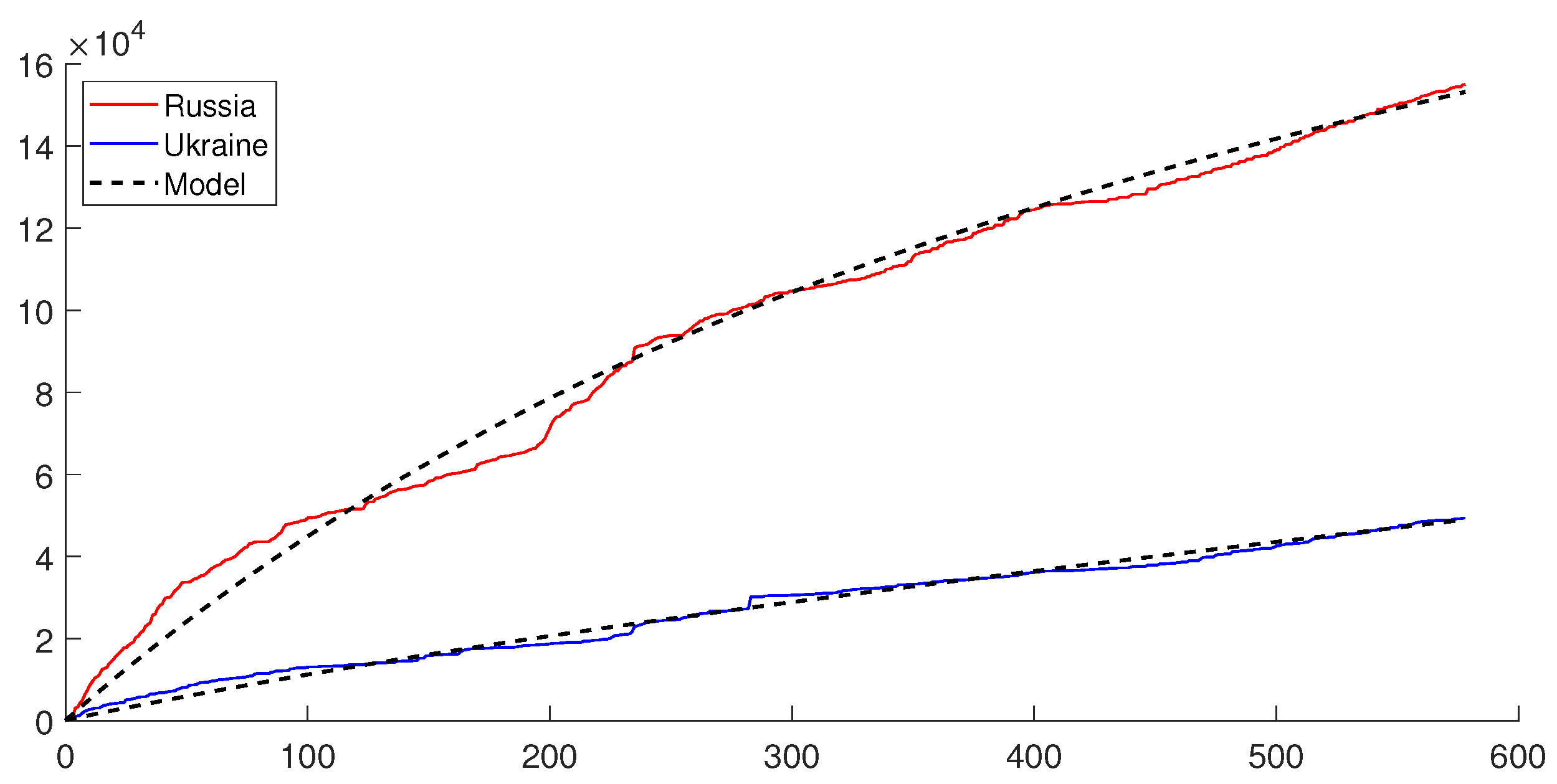
The aggregate plot of the simulations over the entire period is presented in Figure 4. In Table 2, we summarize the mean relative errors
MRE ( x d a t a , x s i m u l ) : = 1 N j = 1 N | ( x d a t a ( t j ) x s i m u l ( t j ) ) / ( x d a t a ( t j ) + ϵ ) |
between the data x d a t a and the simulations x s i m u l . In our simulation, we set ϵ = 1 . To validate the improvement in data fitting performance achieved by the proposed approach, we tested the SINDy algorithm without data partitioning, which resulted in a single model with coefficients
a 1 = 5.1789 × 10 2 , b 1 = 4.6750 × 10 3 , c 1 = 6.8759 × 10 3 , a 2 = 1.2181 × 10 2 , b 2 = 8.6829 × 10 4 , c 2 = 1.6349 × 10 3 .
This model is illustrated in Figure 5. The effectiveness of the proposed method can be assessed by comparing Figure 4 and Figure 5. The mean relative errors for the model with coefficients (14) are 6.9007 × 10 2 and 7.8420 × 10 2 for Russia and Ukraine, respectively. These values are over three times larger than the corresponding average errors of the proposed method, which are 1.8712 × 10 2 and 1.6154 × 10 2 for Russia and Ukraine, respectively.

7. Conclusions

In this study, we embarked on a journey to bridge the historical foundations of combat modeling, epitomized by the Lanchester model, with the intricate dynamics of contemporary warfare, exemplified by the Russia–Ukraine war. The persistent need to comprehend the essence of war and predict its outcomes propelled us to explore innovative methodologies, particularly the Sparse Identification of Nonlinear Dynamics (SINDy) algorithm, to enhance the applicability and adaptability of the Lanchester model in the face of modern complexities. Our application of SINDy to armor-centric combat loss data from the ongoing Russia–Ukraine war has yielded insightful results. The algorithm, operating without prior knowledge of the system’s dynamics, successfully identified governing equations for the Lanchester model, specifically tailored to the attrition data of combat equipment. This approach not only overcomes the challenges posed by the nonlinear and analytically complex nature of the modern warfare dynamics but also provides a pathway for efficient simulation and analysis.
Our proposed method, outlined in Section 5, strategically partitioned the time-series data and employed SINDy for system identification, enhancing the fidelity of the model to the dynamic nature of the conflict. The subsequent simulations, discussed in Section 6, provided a nuanced understanding of the dynamics, offering valuable insights into the evolving nature of warfare in the Russia–Ukraine war. Despite this, the MLS and SINDy algorithms utilized in the current study have limitations. It is not easy to preserve abrupt changes in data because the MLS smoothing uses the same weights for every evaluation. The derivative values required for applying the SINDy method are estimated from measurement data using a simple finite difference, which may lead to degraded performance under noisy circumstances, as discussed in [24]. To obtain more accurate results, we can enhance the current versions of MLS and SINDy by incorporating data-adapted weights and employing more sophisticated techniques to estimate derivatives, respectively. This issue could be addressed through a more in-depth investigation into combat scenarios and the geometric characteristics of the data. Such research endeavors have the potential to provide a basis for more sophisticated analysis and predictions of combat performance. It is our intention to address these challenges in future research, aiming to contribute solutions that enhance the precision of analysis and predictions related to combat effectiveness.

Author Contributions

Conceptualization, D.C.; methodology, D.C. and B.J.; software, B.J.; validation, D.C. and B.J.; formal analysis, D.C.; investigation, B.J.; resources, D.C.; data curation, D.C.; writing—original draft preparation, D.C. and B.J.; writing—review and editing, D.C. and B.J.; visualization, B.J.; supervision, D.C.; project administration, D.C.; funding acquisition, B.J. All authors have read and agreed to the published version of the manuscript.

Funding

This research was supported by the Bisa Research Grant of Keimyung University in 2022.

Data Availability Statement

Conflicts of Interest

The authors declare no conflicts of interest.

References

  1. Lanchester, F.W. Aircraft in Warfare: The Dawn of the Fourth Arm, 1st ed.; Constable and Co.: London, UK, 1916. [Google Scholar]
  2. Morse, P.M.; Kimball, G.E. Methods of Operations Research, 1st ed.; John Wiley: New York, NY, USA, 1951. [Google Scholar]
  3. Weiss, H.K. Combat Models and Historical Data: The U.S. Civil War. Oper. Res. 1966, 14, 759–790. [Google Scholar] [CrossRef]
  4. Peterson, R. On the Logarithmic Law of Combat and Its Application to Tank Combat. Oper. Res. 1967, 15, 557–558. [Google Scholar] [CrossRef]
  5. Dietchman, S.J. A Lanchester Model of Guerrilla Warfare. Oper. Res. 1962, 10, 818–827. [Google Scholar] [CrossRef]
  6. Schaffer, M.B. Lanchester Models of Guerrilla Engagements. Oper. Res. 1968, 16, 457–488. [Google Scholar] [CrossRef]
  7. Hartley, D.S.; Helmbold, R.S. Validating Lanchester’s square law and other attrition models. Nav. Res. Log. 1995, 42, 609–633. [Google Scholar] [CrossRef]
  8. Kress, M. Lanchester Models for Irregular Warfare. Mathematics 2020, 8, 737. [Google Scholar] [CrossRef]
  9. Cangiotti, N.; Capolli, M.; Sensi, M. A generalization of unaimed fire Lanchester’s model in multi-battle warfare. Oper. Res. Int. J. 2023, 23, 38. [Google Scholar] [CrossRef]
  10. Keane, T. Combat modelling with partial differential equations. Appl. Math. Model. 2011, 35, 2723–2735. [Google Scholar] [CrossRef]
  11. Coulson, S.G. Lanchester modelling of intelligence in combat. IMA J. Manag. Math. 2019, 30, 149–164. [Google Scholar] [CrossRef]
  12. Spradlin, C.; Spradlin, G. Lanchester’s equations in three dimensions. Comput. Math. Appl. 2007, 35, 999–1011. [Google Scholar] [CrossRef]
  13. Clifton, E. A brief review on the application of Lanchester’s models of combat in nonhuman animals. Ecol. Psychol. 2020, 32, 181–191. [Google Scholar] [CrossRef]
  14. Johnson, D.D.P.; MacKay, N.J. Fight the Power: Lanchester’s laws of combat in human evolution. Evol. Hum. Behav. 2013, 36, 152–163. [Google Scholar] [CrossRef]
  15. Jørgensen, S.; Sigué, S. A Lanchester-Type Dynamic Game of Advertising and Pricing. In Games in Management Science; Sigue, P.-O., Taboubi, S., Pineau, S., Eds.; Springer: New York, NY, USA, 2020; pp. 1–14. [Google Scholar]
  16. Stanescu, M.; Barriga, N.; Buro, M. Using Lanchester Attrition Laws for Combat Prediction in StarCraft. In Proceedings of the Eleventh AAAI Conference on Artificial Intelligence and Interactive Digital Entertainment (AIIDE-15), Santa Cruz, CA, USA, 14–18 November 2015; pp. 86–92. [Google Scholar]
  17. Brunton, S.L.; Proctor, J.L.; Kutz, J.N. Discovering governing equations from data by sparse identification of nonlinear dynamical systems. Natl. Acad. Sci. USA 2020, 113, 3932–3937. [Google Scholar] [CrossRef]
  18. Jiang, Y.-X.; Xiong, X.; Zhang, S.; Wang, J.-X.; Li, J.-C.; Du, L. Modeling and prediction of the transmission dynamics of COVID-19 based on the SINDy-LM method. Nonlinear Dyn. 2021, 105, 2775–2794. [Google Scholar] [CrossRef]
  19. Lakshminarayana, S.; Sthapit, S.; Maple, C. Application of Physics-Informed Machine Learning Techniques for Power Grid Parameter Estimation. Sustainability 2022, 14, 2051. [Google Scholar] [CrossRef]
  20. Ren, Y.; Adams, C.; Melz, T. Uncertainty Analysis and Experimental Validation of Identifying the Governing Equation of an Oscillator Using Sparse Regression. Appl. Sci. 2022, 12, 747. [Google Scholar] [CrossRef]
  21. Wei, B. Sparse dynamical system identification with simultaneous structural parameters and initial condition estimation. Chaos, Solitons Fractals 2022, 165, 112866. [Google Scholar] [CrossRef]
  22. Ayankoso, S.; Olejnik, P. Time-Series Machine Learning Techniques for Modeling and Identification of Mechatronic Systems with Friction: A Review and Real Application. Electronics 2023, 12, 3669. [Google Scholar] [CrossRef]
  23. Dong, X.; Bai, Y.-L.; Lu, Y.; Fan, M. An improved sparse identification of nonlinear dynamics with Akaike information criterion and group sparsity. Nonlinear Dyn. 2023, 111, 1485–1510. [Google Scholar] [CrossRef]
  24. Champion, K.P.; Brunton, S.L.; Kutz, J.N. Discovery of Nonlinear Multiscale Systems: Sampling Strategies and Embeddings. SIAM J. Appl. Dyn. Syst. 2019, 18, 312–333. [Google Scholar] [CrossRef]
  25. Oryx’ Site. Available online: https://www.oryxspioenkop.com/2022/02/attack-on-europe-documenting-equipment.html (accessed on 1 August 2023).
  26. Turkes, T. Fitting Lanchester and Other Equations to the Battle of Kursk Data. Master’s Thesis, Naval Postgraduate School, Monterey, CA, USA, March 2000. [Google Scholar]
  27. Zhang, L.; Schaeffer, H. On the convergence of the SINDy algorithm. Multiscale Model. Simul. 2019, 17, 948–972. [Google Scholar] [CrossRef]
  28. Levin, D. The approximation power of moving least-squares. Math. Comput. 1998, 67, 1517–1531. [Google Scholar] [CrossRef]
  29. Allen, L. An Introduction to Mathematical Biology; Pearson: Upper Saddle River, NJ, USA, 2006. [Google Scholar]
  30. Duffey, R.B. Dynamic theory of losses in wars and conflicts. Eur. J. Oper. Res. 2017, 261, 1013–1027. [Google Scholar] [CrossRef]
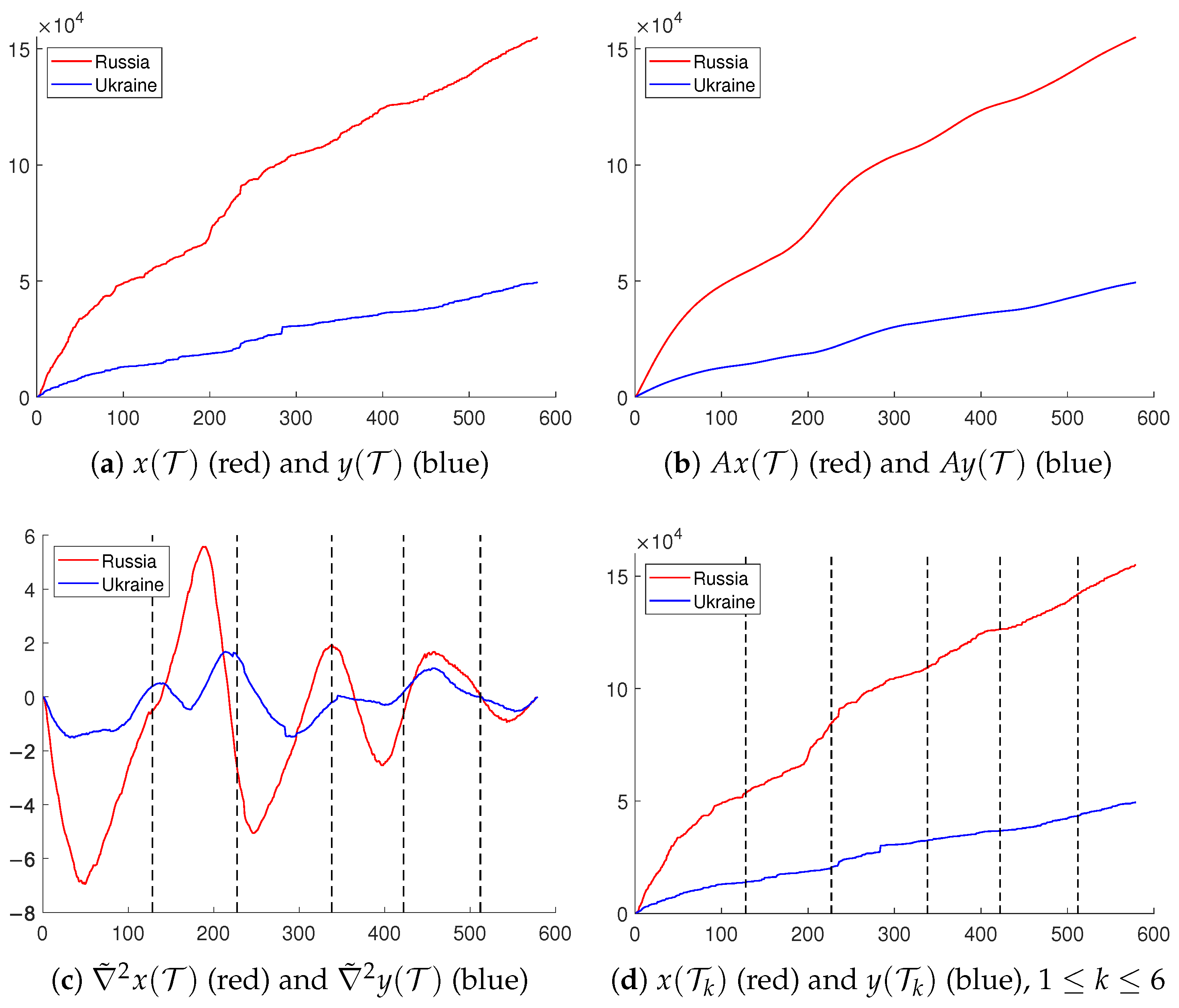
Figure 1. Partition of the cumulative loss data: dotted lines visualize the partition.
Mathematics 12 00851 g001
Figure 2. Models over the six subsets of measurement times, T k , k = 1 , 2 , , 6 : cumulative losses of Russian forces (red), Ukrainian forces (blue), and models (black dashed).
Mathematics 12 00851 g002
Figure 3. Ratio x / y of loss rates over the six subsets of measurement times, T k , k = 1 , 2 , , 6 .
Mathematics 12 00851 g003
Figure 4. Aggregated model over the entire time period: cumulative losses of Russian force (red), Ukrainian force (blue), and model (black dashed).
Mathematics 12 00851 g004
Figure 5. Model with coefficients in (14) obtained by the SINDy algorithm without partitioning of data: cumulative losses of Russian force (red), Ukrainian force (blue), and model (black dashed).
Mathematics 12 00851 g005
Table 1. Equipment types and weights for measuring combat losses.
Equipment TypesWeightsEquipments
Tanks40Tanks
Self-Propelled Tank Missile Systems
Artillery20Artillery
Self-Propelled Artillery
Towed Artillery
Multiple Rocket Launchers
Artillery Support Vehicles Furthermore, Equipment
Armored Vehicles5Armoured Fighting Vehicles
Armoured Personnel Carriers
Infantry Fighting Vehicles
Infantry Mobility Vehicles
Mine-Resistant Ambush Protected
Support Equipments5Command Posts
Communications Stations
Communications Vehicles
Engineering Vehicles Furthermore, Equipment
Anti-tank Personal Firearms and Mortars3Anti-Tank Guided Missiles
Mortars
Other Combat Vehicles3Trucks
Vehicles and Jeeps
Table 2. Mean relative errors (13) between the data and the model over subsets of times in (10).
Time SubsetErrors of RussiaErrors of Ukraine
T 1 6.1514 × 10 2 3.4004 × 10 2
T 2 1.6780 × 10 2 1.4301 × 10 2
T 3 6.0071 × 10 3 2.2299 × 10 2
T 4 3.0560 × 10 3 3.8061 × 10 3
T 5 2.8975 × 10 3 5.7214 × 10 3
T 6 2.5939 × 10 3 4.5478 × 10 3
Disclaimer/Publisher’s Note: The statements, opinions and data contained in all publications are solely those of the individual author(s) and contributor(s) and not of MDPI and/or the editor(s). MDPI and/or the editor(s) disclaim responsibility for any injury to people or property resulting from any ideas, methods, instructions or products referred to in the content.