Optimization of Personal Credit Evaluation Based on a Federated Deep Learning Model

Abstract

Financial institutions utilize data for the intelligent assessment of personal credit. However, the privacy of financial data is gradually increasing, and the training data of a single financial institution may exhibit problems regarding low data volume and poor data quality. Herein, by fusing federated learning with deep learning (FL-DL), we innovatively propose a dynamic communication algorithm and an adaptive aggregation algorithm as means of effectively solving the following problems, which are associated with personal credit evaluation: data privacy protection, distributed computing, and distributed storage. The dynamic communication algorithm utilizes a combination of fixed communication intervals and constrained variable intervals, which enables the federated system to utilize multiple communication intervals in a single learning task; thus, the performance of personal credit assessment models is enhanced. The adaptive aggregation algorithm proposes a novel aggregation weight formula. This algorithm enables the aggregation weights to be automatically updated, and it enhances the accuracy of individual credit assessment by exploiting the interplay between global and local models, which entails placing an additional but small computational burden on the powerful server side rather than on the resource-constrained client side. Finally, with regard to both algorithms and the FL-DL model, experiments and analyses are conducted using Lending Club financial company data; the results of the analysis indicate that both algorithms outperform the algorithms that are being compared and that the FL-DL model outperforms the advanced learning model.

1. Introduction

The development of internet finance has led to a dramatic increase in personal credit data; however, the models that are derived from the training of most financial institutions, which are based on only their own data sets, are overfit for practical applications, and they cannot effectively identify defaulted loan information. Consequently, a substantial increase in the default rate of various loan operations has occurred, and to a certain extent, confusion has occurred in the financial market. Meanwhile, because credit financial data exhibit somewhat high-dimensional and high-noise characteristics, financial institutions began to continuously utilize novel learning methods; thus, they aimed to enhance the accuracy of personal credit evaluation models.

A large number of scholars have considered enhancing the accuracy of personal credit assessment models. In 2014, Stjepan Oreski et al. [1] observed that the data analyzed by current financial institutions are high-dimensional data, and they noted that the existence of numerous irrelevant features may reduce the prediction accuracy of neural networks. Stjepan Oreski et al. selected crucial data preprocessing features through genetic algorithms, and they utilized neural network modeling. Their experimental results indicated that the accuracy of credit evaluation models can be enhanced using feature selection techniques. In 2018, Yashna Sayjadah et al. [2] compared the prediction accuracy of logistic regression, decision tree, and random forest algorithms, and they considered credit data; the results indicated that random forest exhibits a high accuracy rate. Linear statistical methods such as logistic regression do not exhibit a good fit for the current complex, multidimensional, and nonlinear financial credit data; traditional neural networks exhibit high requirements for the dimensionality and amount of data, and random forests require a certain level of data volume to obtain more desirable results. Due to the development of computing device performance, the deep learning capability of convolutional neural networks has been widely observed in recent years, and increasingly complex and expressive network models, such as VGGNet [3], DenseNet [4], and MobileNet [5], have emerged. These models are also utilized for personal credit evaluation; however, in regard to overall quantity and data dimensionality, the data available to a single financial institution are limited. Thus, the information learned from a limited data set is not accurate enough for a large and complex real-world market. To address the problems of privacy leakage and a lack of device performance, which is associated with learning tasks, the authors propose a federated deep learning model.

Federated learning is a distributed setup that enables each client to collaboratively train a federated global model while locally keeping the data. Thus, federated learning exhibits private data protection, distributed computation, and distributed storage. In regard to the research on federated learning systems, both communication and aggregation represent crucial and relevant performance bottlenecks [6]. Deep learning, which is a type of machine learning algorithm, is a technique through which machine learning can be implemented, and typical algorithms include deep belief networks (DBN) [7], convolutional neural networks (CNN), and recursive neural networks (RNN) [8]. Unlike traditional machine learning algorithms that usually focus on pre-built “feature engineering”, deep learning can automatically learn “feature engineering”, which is also referred to as “feature detectors” [9]. By effectively combining federated learning and deep learning with the advantages of nonlinear mapping and parallel processing, federated deep learning learns the multidimensional complex features of financial loan data through its own network structure, and it automatically adjusts the internal large number of connection weights to accurately fit the data features. The self-organization, self-learning, superb memory, and high fault tolerance capabilities that characterize federated deep learning are suitable for processing the current multidimensional and highly noisy nonlinear data such as credit data.

The subsequent research structure is as follows. First, by classifying major approaches to personal credit evaluation, as well as their advantages and disadvantages, and background knowledge, key techniques, such as federated learning, incremental learning, and deep learning are introduced. Subsequently, to solve the key problems associated with federated learning, a dynamic communication algorithm and adaptive aggregation algorithm are proposed. Thus, the FL-DL model architecture is constructed, and the pseudo-code description is provided. Subsequently, using relevant data obtained from financial institutions, the constructed FL-DL model is analyzed, and by comparing four related models, the accuracy of the FL-DL model is verified. Finally, through the conclusion of the analysis of the FL-DL model, the next research direction is proposed.

This study enhances the scenario that is characterized by the following problems: susceptibility to adopting local optimal solutions, privacy leakage, and the insufficient device performance that may characterize other personal credit assessment models. The FL-DL model can enhance the prediction accuracy and convergence speed of the model; this enhancement entails adopting the distributed architecture of federated deep learning for modeling, which solves the data silo problem of financial institutions and achieves the goal of secure joint modeling by multiple financial institutions using local credit data without disclosing data privacy.

2. Background Knowledge and Key Technologies

Federated deep learning, an emerging data mining algorithm, exhibits a wide range of applications in the field of credit evaluation, and in regard to the limited-data scenario, it is able to build models with excellent performance.

2.1. Main Assessment Methods for Personal Credit

The main methods for personal credit evaluation are statistical learning and machine learning (

Table 1. Comparison of Personal Credit Evaluation Methods.

Methodology	Advantages	Disadvantages
LDA	Reduce the subjectivity of manual credit assessment discriminations	Presence of parameter estimation sample selection bias
K-nn	The overall idea is simple, and the effect is powerful. Utilized to solve regression problems	Cannot avoid the problem of “dimensional disaster” occasioned by high-dimensional data
LR	The independent variables do not need to conform to the normal distribution between the samples without the same distribution between the requirements	The requirement that the feature space is not very large, and it requires data without missing and wrong data
LP	Linear processing with satisfactory accuracy evaluation	High subjectivity of indicator classification
Bayesian network	Strong interpretability of classification results, handling both stereotypical and quantitative attributes	Weak evaluation power when correlation between attributes are high
CNN	Suitable for high-dimensional, nonlinear, noise-laden data	Susceptible to local minima; not determinable for the parameters of the neural network
SVM	Avoids non-linearity, “dimensional disasters”, etc.	Inefficient computation of large amounts of data
DT	No distribution requirement for sample data; strong generalization ability	Difficult to handle data with a wide range of fluctuations
Aprioi	Mineable correlations between attributes	Low computational efficiency
Fuzzy	Can reflect the relative importance of the evaluation indicators, making the comprehensive evaluation results more scientific and reasonable	There may be subjectivity in setting the weights, which makes the comprehensive evaluation results have certain deviations

), among which the method of assessing personal credit using mathematical statistics cannot be effectively applied for high-dimensional sparse and noisy credit data, as this method has poor mapping ability for nonlinear data. By contrast, machine language exhibits a strong nonlinear mapping capability; thus, the requirements for data features and ranges are reduced, and it can also be applied to sparse and noisy data. Therefore, this study utilizes machine learning as the basic model for personal credit evaluation.

2.2. Federated Learning

Federated learning, a distributed setup proposed by McMahan et al. [10] in 2017, enables clients to collaboratively train a federated global model; simultaneously, it enables them to locally store data on their devices. Federated learning enables the decentralized clients to collaboratively train a shared global model without sharing local data. Thus, the goals of privacy preservation, distributed computing, and storage are achieved. Federated learning is divided into horizontal federated learning [11], vertical federated learning [12], and federated migration learning [13].

Federated learning comprises a server side and multiple clients. Figure 1 indicates that where the arrows connecting the server side to each client represent the communication process, the blue arrow represents the scenario in which each client is sending a local model to the server side, and the green arrow represents the server side broadcasting a global model to each client. In the federated learning system, the server side is mainly responsible for two tasks. First, it selects the clients at the beginning of training, and it broadcasts the initial global model to each client; second, with regard to forming a new global model, it is responsible for aggregating the received local models and for subsequently broadcasting the new global model to each client during the subsequent training. The decentralized clients are responsible for independently training the models broadcasted on the server side using the privacy data and for retransmitting the trained model parameters to the server side.

Multiple data transfers between the server side and each client are required; in federated learning, this phenomenon is known as communication. Typically, the clients that constitute a federated learning system synchronously communicate with the server; each client locally sends the trained model parameters to the server after a fixed number of training rounds. Furthermore, the server generates a new global model, and it distributes it to the clients for further training. It is commonly accepted that the cost of cross-device communication is often much higher than the cost of communication within or between data centers. Therefore, in regard to practically applying federated learning systems, because communication represents a major performance bottleneck, it exhibits immense practical importance.

In addition, using an algorithm, the server side aggregates the received local models of each decentralized training into a global model, which is the tool utilized to finally evaluate the learning effectiveness of the system. Therefore, aggregation, which is closely linked with communication, is another bottleneck affecting the performance of federated learning systems, and with respect to the federated learning field, it is a major research topic. Most of the current state-of-the-art research aggregates each dispersed client model by averaging the parameters; however, none of these studies can theoretically explain why averaging is an effective approach. Therefore, research on designing more effective aggregation algorithms is a crucial research direction for federated learning. The standard federated learning model [14], which is depicted in Algorithm 1, provides the basis for the current research.

Algorithm 1 Federated average algorithm.

Server side:   1: Initialize $G{M}_0$   2: for epoch t in range (0, E) do   3:    for client k in range (n) do   4:       $M_k^t$← ClientShare $(k,G{M}_t)$   5:    end for   6:    $G{M}_{t+1}\leftarrow N_k/N{\sum }_{k=1}^n{M}_k^t$   7: end for   ClientShare $(k,GM)$:   8: $\beta \leftarrow$ Assign $D_k$ randomly by size B   9: for client batch $b\in \beta$ do 10:    $M_k⟵GM-\nabla L(M_k,b)$ 11: end for 12: return $M_p$

Here, the federated average algorithm n represents the total number of clients in the system, $D_k$ represents the local training set of client k, $N_k$ represents the size of the local data set $D_k$ of client k, N represents the size of the whole data set, $M_k$ represents the local model of client k, B represents the minimum batch size for local training, E represents the total number of training iterations, and $\eta$ represents the learning rate.

2.3. Incremental Learning

A satisfactory machine learning algorithm should be interpretable and generalizable. When the amount of training data is immensely small, the model may not learn sufficiently, and because its knowledge may become limited to a small population, generalizability cannot be satisfied. Incremental learning is an approach that incrementally updates knowledge without forgetting, and it can solve the problem of not being able to obtain all the data at once, which characterizes realistic tasks. Thus, when subjected to multiple batches of small data sets, it exhibits effective performance. In scientific research, it is common to obtain all the training data at once and to train these data in batches; thus, a model can be obtained. However, real-life tasks do not always exhibit once-and-for-all characteristics, and the data pertaining to these tasks are often obtained progressively. Therefore, it is unrealistic to wait until the right amount of data is collected before learning. Such an action negates the original purpose of artificial intelligence: enhancing the convenience of human life.

Similar to other AI methods, incremental learning aims to simulate human thinking. Imagine that when we have learned the knowledge point (1) “1 + 1 = 2”, we do not need to learn the knowledge point (2) “2 × (1 + 1) = ?”. We do not need to learn point (1) again because it has been mastered before. This is the goal of incremental learning, which is subject to the “catastrophic forgetting” dilemma (i.e., how to ensure that new knowledge is learned without forgetting what has already been learned and without reusing the data already learned). Figure 2 indicates that the common incremental learning methods are divided into three categories [14]: fine-tuning, joint training, and feature extraction methods.

Figure 2A indicates that for the original multitask learning model, the test data are tested once on each old task. The fine-tuning method [15] initializes the parameters of the new model to those of the old one, and when training the new model, it fine-tunes some of the parameters. This commonly utilized method is intermediate; it represents the phase between feature extraction and joint training. Figure 2B indicates that when a new task appears, the gray legend represents the fine-tuned part of the parameters contained on the old model, and the yellow legend represents the fine-tuned new model. The joint training method [16] is depicted in Figure 2C. Whenever a new task appears, the aforementioned method feeds all the data from the old task and the new task into the model for retraining, which also represents the centralized training concept. This is apparently the most effective method; however, it is temporally and spatially expensive.The feature extraction method [17] can bridge the old and new tasks by extracting some of the features on the trained model of the old task and applying them to the new task for training. Figure 2D indicates that when there is a new task, the white legend represents the unchanged old model, and the yellow one represents the new model with some features applied to the old model.

2.4. Deep Learning

Deep learning (DL) is a technique for implementing machine learning; however, unlike traditional machine learning algorithms that focus on pre-built “feature engineering”, it is able to automatically learn “feature engineering” [18]. The performance of a DL algorithm model is proportional to the amount of trained data; the larger the amount of training data, the stronger the model performance. However, an implicit condition exists: the algorithm can model an infinite range of growth. Because the model size can be made as large as possible, the model can accommodate more tensor space for data representation, which is apparently unrealistic in terminal devices and edge devices with limited computation and storage capacity. Therefore, research on DL acceleration algorithms is crucial. Figure 3 illustrates the basic approach of DL methods.

3. Federated Deep Learning Model Construction

To enhance the accuracy of the evaluation model, which is a function of federated learning, this subsection proposes a dynamic communication algorithm and an adaptive aggregation algorithm. Subsequently, the federated deep learning model (FL-DL) is constructed based on the two aforementioned algorithms.

3.1. Dynamic Communication Algorithm Design

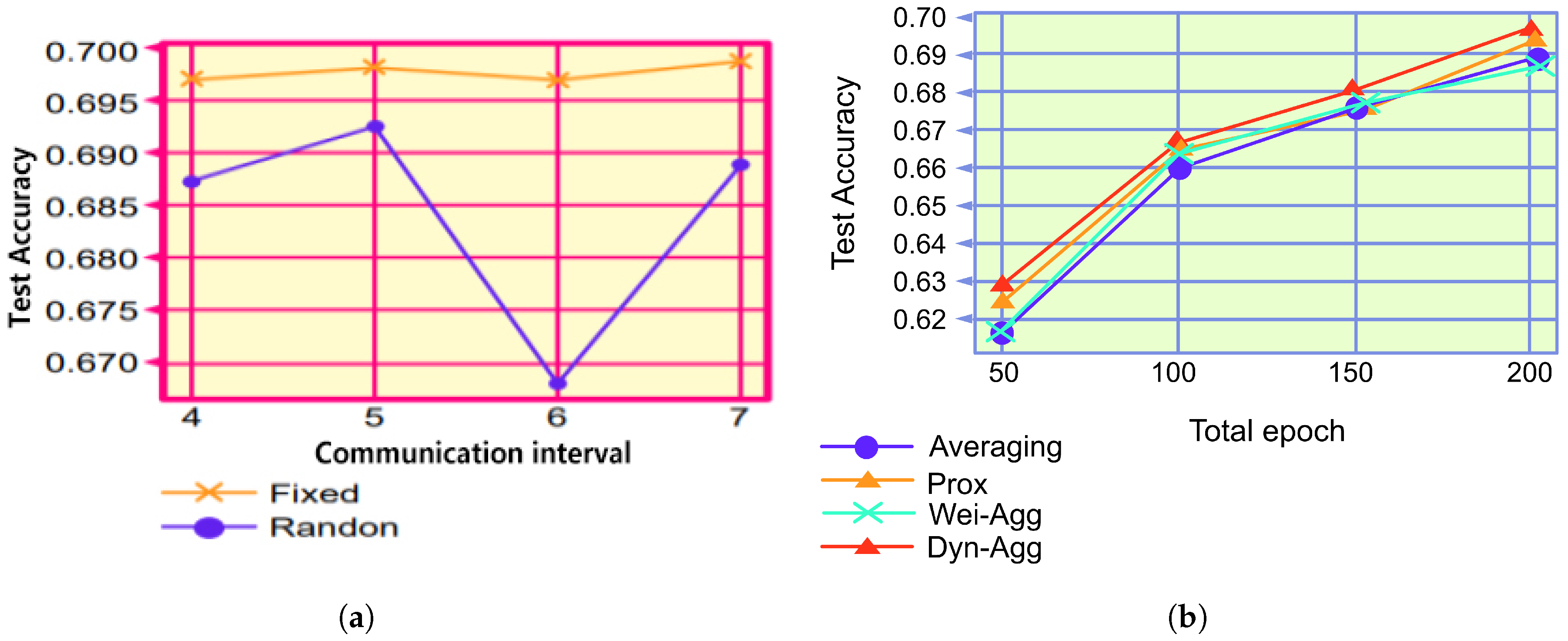
It is difficult to predict and utilize a suitable communication interval before training, and an inappropriate communication interval can adversely affect model performance [19]; therefore, a dynamic communication interval is considered. With respect to the federated learning system, we utilize a fixed communication interval in the first half-cycle of the training. Therefore, the system follows a fixed communication scheme. Subsequently, it utilizes a variable communication interval in the second half cycle. Larger communication intervals can lead to a decrease in task accuracy [20]; to address this problem, the dynamic communication algorithm adds a constraint to the variable communication interval. Thus, it prevents the communication interval from becoming immensely large. By using the constrained variable communication interval, the federated learning system follows the dynamic communication scheme in the second half cycle of training. This combination (i.e., making the federated learning system utilize a fixed communication scheme in the first half-cycle of training and a dynamic communication scheme in the second half-cycle) constitutes the dynamic communication algorithm proposed herein.

Let the total number of system training wheels be E, the fixed communication interval be f, the set of training wheels be $se{t}_t=\left\{t\in N^{*}|1\le t\le E\right\}$, the set of communication occurring wheels be $set{}_e$, and the set of communication intervals be $se{t}_{int}$. The dynamic communication algorithm is described as follows:

Step 1: Divide set ${}_t$ into three subsets of training wheels based on the fixed communication interval f and the midpoint $\lfloor E/2\rfloor$ of the total training period. Because f is not necessarily divisible by E in practical applications, the three divided subsets are as follows: ${set}_{t1}=\left[1,{\lfloor 1,E/2f\rfloor }^{*}f\right]$, set${}_{t2}=[{\lfloor E/2f\rfloor }^{*}f,{\lfloor E/f\rfloor }^{*}f]$, and ${set}_{t3}=[{\lfloor E/f\rfloor }^{*}f,E]$.

Step 2: Construct the communication interval set $se{t}_{int}$ based on the three training wheel subsets.

For ${set}_{t1}$, for each $t\in {set}_{t1}$, and for $t/f=0$, an f is added to ${set}_{int}$. It is apparent that by this operation, the algorithm adds a total number of $\lfloor E/2f\rfloor f$s to ${set}_{int}$ at $t\in {set}_{t1}$.

For ${set}_{t2}$, for each $t\in {set}_{t2}$, and for $t/f=0$, the algorithm randomly selects an integer in the interval $\left(t^{*}f-f,t^{*}f\right]$ of length f; thus, it replaces the original communication-generating wheel $t^{*}f$ and adds it to $se{t}_e$. After each addition of the randomly selected communication-generating wheel to set $t_e$, the algorithm computes the difference between the value of the last element in set $t_e$ that is not 0 and the value of its predecessor element, and it adds the computed difference to $se{t}_{int}$. Let the value of the predecessor element pertaining to the first element in $se{t}_e$ be 0. 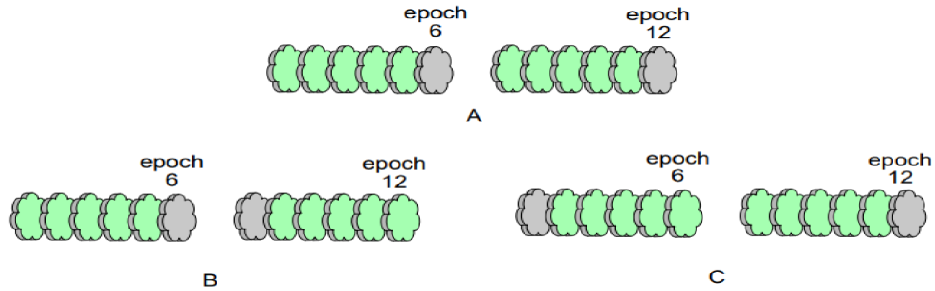By restricting the selection of the alternative communication-generating wheels to the left side of the replaced original communication-generating wheel (i.e., the $t^{*}f$-th wheel) to a left-open–right-closed position of length f, the interval between the two alternative communication-generating wheels (i.e., the variable communication interval) is made to be no more than $(2f-1)$ and no less than 1; thus, a constraint is added to the variable communication interval to prevent it from varying considerably and from occasioning the degradation of the model performance. As per Figure 4, let the fixed communication interval be 6. Figure 4A depicts the communication generation wheels of rounds 6 and 12 when the fixed communication interval is utilized, Figure 4B indicates the minimum interval case when the variable communication interval is utilized, and Figure 4C indicates the maximum interval case when the variable communication interval is utilized.

For ${set}_{t3}$, it is apparent that if f is divisible by E, then it will not exist. If f is not divisible by E, for any $t\in {set}_{t3}$, the federated learning system that follows the fixed communication scheme is not communicating. Therefore, to accurately compare the dynamic communication algorithm proposed herein with the federated learning algorithm that follows the original fixed communication scheme, the dynamic communication algorithm does not treat ${set}_{t3}$.

Step 3: Apply the constructed $se{t}_{int}$ to the server side. The server side takes one element from $se{t}_{int}$ and broadcasts it sequentially and without putting it back each time it broadcasts global model parameters to the clients. Subsequently, each client sets the value of the broadcasted element to the number of local training rounds, and the local private data set is utilized to train the global model.

Using the three aforementioned steps, the federated learning system that applies the dynamic communication algorithm will follow a fixed communication scheme during the first half-cycle of training, and it will follow a dynamic communication scheme during the second half-cycle of training. The dynamic scheme can optimally combine the two schemes; thus, an enhanced model performance is obtained. This combined approach is the dynamic communication approach (Algorithm 2).

In the scenario in which the total number of training rounds is E and the fixed communication interval is f, the dynamic communication algorithm first initializes the “midpoint” round ${\lfloor E/2f\rfloor }^{*}f$, the set of communication occurring rounds $se{t}_e$, the set of communication intervals $se{t}_{int}$, and the two self-increasing variables i and j. Subsequently, $se{t}_e$ and $se{t}_{int}$ are calculated as per the preceding three steps and the corresponding three scenarios contained in Algorithm 2. Finally, $se{t}_{int}$ is output.

Algorithm 2 Dynamic communication algorithm

1: Input: total number of training rounds of System E, fixed communication interval f 2: Initialize the “midpoint” round ${\lfloor E/2f\rfloor }^{*}f$ for division, $se{t}_e\left[1\right]=0$ for the set of communication occurring rounds, ${set}_{int}$ for the set of communication intervals, and self-incrementing variables $i=1$ and $j=1$ 3: for t in range (1, E) do: 4:      if $1\le t\le {\lfloor E/2f\rfloor }^{*}f$ and $t/f==0$:         $se{t}_{int}\left[i++\right]=f$ 5:      elif $t=={\lfloor E/2f\rfloor }^{*}f+2:$ # “randint$(a,b]$” means to choose a random integer in the interval $(a,b)$           ${set}_e{[++j]=randint(\lfloor E/2\rfloor }^{*}t]$           ${set}_{int}[i++]=se{t}_e\left[i\right]-se{t}_e[i-1]+1$ 6:      elif $t>{\lfloor E/2f\rfloor }^{*}f+2$ and $t/f==0$:        ${set}_e[++j]=randint(t-f,t]$        ${set}_{int}\left[i^{++}\right]={set}_e\left[j\right]-{set}_e[j-1]+1$ 7: Output: $se{t}_{int}$

3.2. Adaptive Aggregation Algorithm Design

Because it has been demonstrated that averaging the weights of the model parameters as per the size of the data set is not the most efficient aggregation method [21], herein, the algorithm that constructs a new aggregation weight formula and automatically updates the aggregation weights is referred to as the adaptive aggregation algorithm. The basic principle of this algorithm is as follows: the automatic updating of aggregation weights is achieved by making the aggregation weights back-propagate and optimize according to the loss of the global model before each use.

First, based on the formula provided by the standard aggregation algorithm FedAvg [22] (i.e., row 6 of Algorithm 1), a novel aggregation weight formula is proposed:

$$GM=\sum _{k=1}^{n}W\left[k\right]·\frac{N_k}{N}·M_k$$

(1)

where $GM$ denotes the global model, n denotes the number of clients, $N_k$ denotes the size of the local data set $D_k$ of client $k,N$ denotes the size of the whole data set, $M_k$ denotes the local model of client k, and $W\left[k\right]$ denotes the aggregation weights proposed for use in $M_k$. The weight $W\left[k\right]$ will be initialized as follows:

$$W\left[k\right]=\frac{ac{c}_k^e·ac{c}_k^e}{{\sum }_{k=1}^{n}ac{c}_k^e·ac{c}_k^e}$$

(2)

where $ac{c}_k^e$ denotes the task accuracy of $M_k$ at the current communication round e. Thus, the adaptive aggregation algorithm extends the impact of the better-performing local model on the global model.

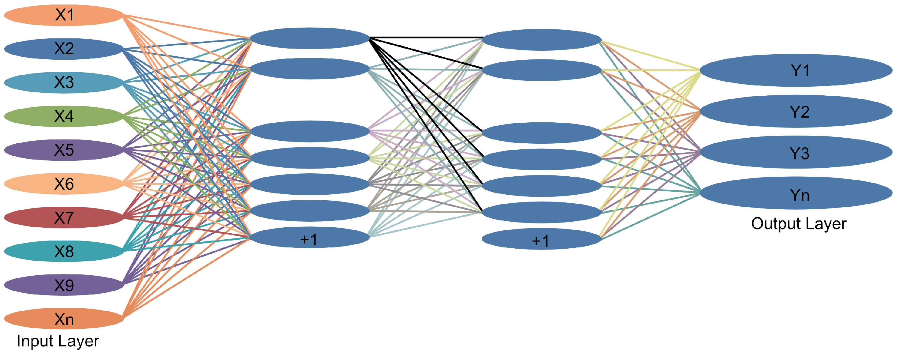
Subsequently, because the feedback mechanism of artificial neural networks enables self-learning [23], a small two-layer neural network, NeuNet (Figure 5), is utilized; thus, the aggregation weights can optimize themselves.

This study considers the manner in which the optimization goal can be set. Because the optimization goal of NeuNet is aligned with the optimization goal of the entire federated learning system, which entails reducing task loss, this study achieves NeuNet self-learning. Therefore, the output layer of NeuNet should be connected to the server side, and this connection is utilized to pass a loss value $SysLoss$ from the server side to the output layer of NeuNet in one direction; thus, $SysLoss$ can be utilized as the loss applied by NeuNet for back propagation. This passed loss value is the average loss of the global model at the end of the last communication (i.e., the average loss of each local model tested on the test set before each local model was trained locally with the global model). This method exhibits the following advantage: it is not necessary to collect the privacy data of each client on the server side to test the global loss, and the method does not add immense computational effort to each client [24]. In summary, the adaptive aggregation algorithm utilizes $W\left[n\right]$ as the input to NeuNet and SysLoss as the back-propagation loss; subsequently, the new $W\left[k\right]$ for client k after automatic optimization is:

$$W\left[k\right]\leftarrow W\left[k\right]-\eta ·\frac{\partial SyLoss}{\partial W\left[k\right]}$$

(3)

where Equation (3) represents the weight update formula of the neural network and $\eta$ denotes the learning rate of NeuNet.

Thus, the adaptive aggregation algorithm complementarily applies the influence of the global model to the local model while expanding the influence of the partial local model on the global model through Equation (2).

The pseudo-code description of the algorithm is depicted in Algorithm 3. The inputs to the adaptive aggregation algorithm are the task accuracy set $SE{T}_{ACC}$ for each local model, the parameter set $SE{T}_M$ for each local model, and the task loss rate set $SE{T}_{Less}$ for the global model. First, the algorithm initializes a two-layer neural network model and the global average loss variable. Subsequently, the global average loss is calculated as per the preceding algorithm description, and the calculated loss is utilized as a feedback for the neural network to automatically update the aggregation weights. Finally, a new global model $GM$ calculated from the new aggregation weights is output.

Algorithm 3 Adaptive aggregation algorithm.

1: Inputs: task accuracy set $SE{T}_{ACC}$ for each local model, parameter set $SE{T}_M$ for each local model, and global model task loss set $SE{T}_{LOSS}$. 2: Initialize a two-layer neural network model $NeuNet$ with global model average loss $SysLoss=0$ 3: for k in range $(1,\left|SE{T}_M\right|+1)$ do:       $acc{k}^{*}acck$ 4:      $W\left[k\right]=\frac{ac{c}_k·ac{c}_k}{{\sum }_{k=1}^{\left|SE{T}_M\right|}ac{c}_k·ac{c}_k}$ 5:      $SysLoss+=SE{T}_{LOSS}\left[k\right]$ 6:      $SysLoss=\frac{SysLos}{\left|SE{T}_M\right|}$ 7: Set $SysLoss$ as the feedback loss of the neural network $NeuNet$ to obtain the automatically optimized $W\left[\left|SE{T}_M\right|\right]$ 8: $GM={\sum }_{k=1}^{\left|SE{T}_M\right|}W\left[k\right]·\frac{N_k}{N}·M_k$ 9: Output: $GM$

3.3. FL-DL Model Design

Based on the dynamic communication algorithm and adaptive aggregation algorithm, this study proposes a new federated learning model (FL-DL), whose framework is depicted in Figure 5.

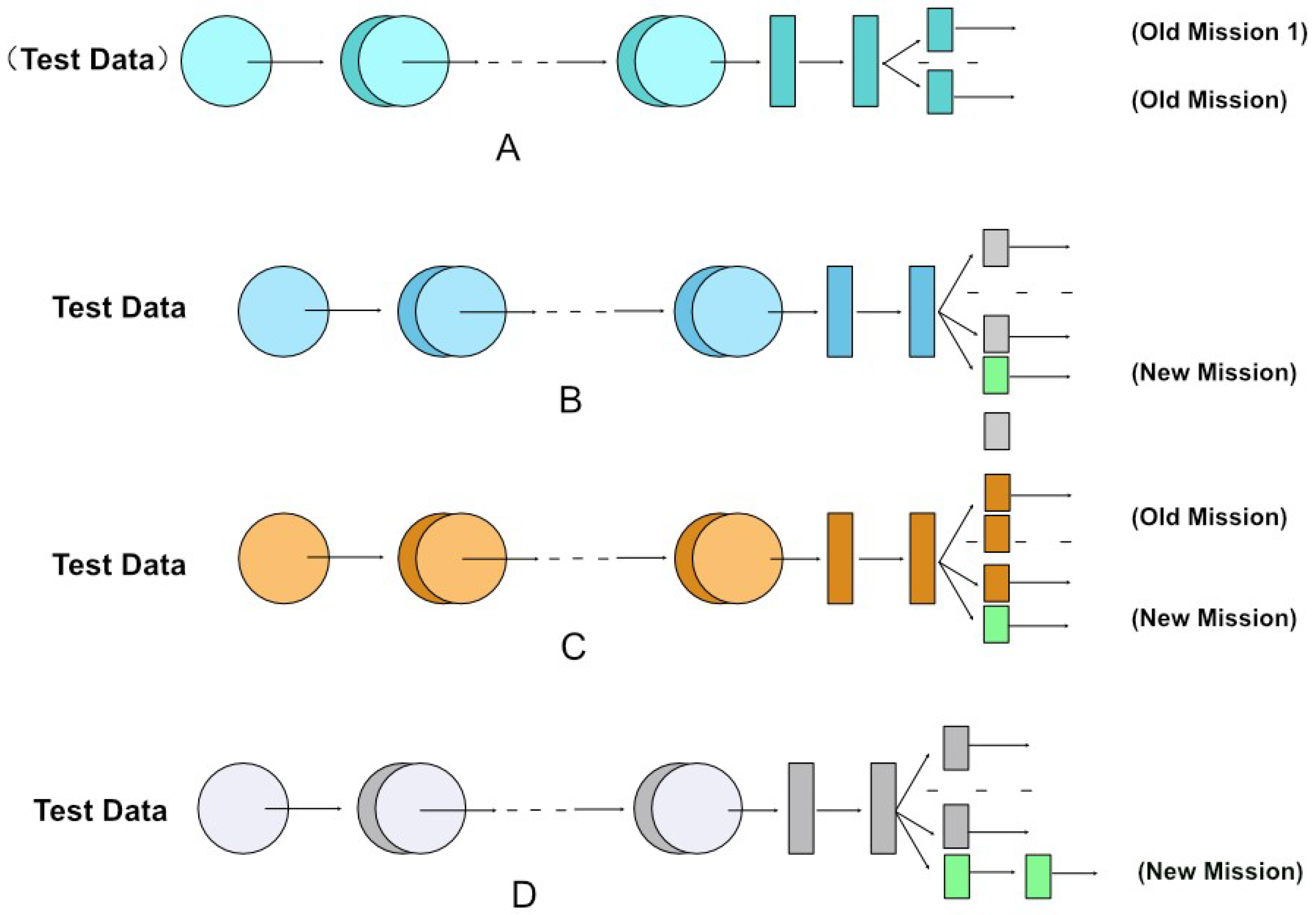
FL-DL is based on the architecture of a typical federated learning system, which comprises a server side and multiple clients. Herein, the same model is utilized for the global model on the server side and for the local model on each client (i.e., both models utilize AlexNet)[25]. It can be observed from the server-side module depicted in Figure 5 that both algorithms proposed herein are applied on the server side, which exhibits the advantage of placing the additional but small computation on the server side instead of on the client side, where computational resources are strained. The pseudo-code description of the model is depicted in Algorithm 4.

Algorithm 4 FL-DL algorithm.

Server side:   1: $if==1$:   2:      Initialize $G{M}_0$   3:      Interval ← Dynamic communication algorithm $\left(E,f\right)$   4: $else$:   5:      Receive the $M_k$ transmitted by each client to build $SE{T}_M,ac{c}_k$ to build $SE{T}_{ACC}$, and $los{s}_k$ to build $SE{T}_{LOSS}$   6:      G M ⟵ Adaptive aggregation $(SE{T}_{ACC},SE{T}_M,SE{T}_{LOSS})$   7: Broadcast the global model $G{M}_0$ or $GM$ and $Interval[i++]$ to each client   Client k:   8: Initialize $Mk\leftarrow GM$, $e\leftarrow Interval$   9: Test the local test set on the global model and obtain the global model loss ${loss}_k^0$ 10: Train the local training set on the global model for e rounds and test it to obtain the accuracy ${loss}_k^0$ of the local model $M_k^{+e}$ 11: Communicate with the server side to transmit ${loss}_k^0,ac{c}_k^{+e},M_k^{+e}$

Here, t represents the training round the system is in; $GM$ represents the global model; Interval represents the set of communication intervals; E represents the total number of training rounds; f represents the fixed communication interval; i represents the self-incrementing variable initialized to zero; $M_k$ represents the local model; $D_k$ represents the local training set of client k; and $T_k$ represents the local test set of client k.

The description of the working steps of FL-DL can be summarized as follows:

Step 1: the server side broadcasts a global model to each client, along with a communication interval $int$ generated by a dynamic communication algorithm;

Step 2: The client first tests the global model on a local test set to obtain the loss of the global model; subsequently, they train the local training set in rounds on the global model, and they test it with the local test set to obtain the local model as well as the task accuracy of the local model;

Step 3: Each client reports the trained local model parameters, the global model loss, and the local task accuracy to the server side;

Step 4: The server side aggregates the local model parameters into a new global model as per the adaptive aggregation algorithm, and it returns to Step 1.

The aforementioned four steps are repeated from round 1, and the new global model is utilized in the next iteration until the number of iterations is $E/f$.

4. Analyzing the Validity and Superiority of the New Model

It is assumed that all participants are honest and that the communication process is ideal, secure, and confidential. This study compares dynamic communication algorithms with typical fixed communication algorithms, and it compares the adaptive aggregation algorithm with the popular FedAvg and FedProx algorithms [26]. It compares the FedDAS model comprising the two proposed algorithms with three advanced federated learning models, namely FedAvg, FedProx, and centralized training. In addition, to ensure the accuracy of the comparison results, among all the compared algorithms or models, the learning models utilize the modern CNN architecture MobileNet.

4.1. Data Set

The data set utilized herein is the credit data set of Lending Club. Lending Club was the first financial company registered with the Securities and Exchange Commission (SEC) to operate a lending business, and it is domiciled in San Francisco. The company lending club offers various types of loans to its customers. When the company receives a loan application, it must decide whether to approve the loan based on the information provided by the applicant. The data set contains information about past loan applicants and whether they have “defaulted” on their loans. Thus, the lender can determine whether a person is likely to default, and different actions can be taken in response to different predictions, such as rejecting the loan application, reducing the loan amount, or lending at a higher interest rate.

The collection of credit data has a person responsible for organizing and maintaining the main aspects, include the following:

• Marital status: Banks prefer customers who are married and in a good relationship with their spouses, as they will have more stability than singles. A bank’s simulated review system shows that, all other things being equal, a married person can receive a whole level of credit enhancement over an unmarried person.
• Technical titles: Borrowers with titles, such as engineers of various grades, economists, accountants, good teachers, etc., are more favored by banks and tend to receive a credit boost.
• Job: Industry practitioners with higher stability can also receive extra points. For example, civil servants, teachers, doctors and employees of some enterprises with good benefits, fashion industry workers, and media people will also be rated on the upper side due to their strong spending power.
• Economic ability: People who provide detailed proof of personal income, stable income, and a long-term outlook for income growth will receive a higher rating.
• Personal housing: Having personal housing also shows that an individual has a certain economic foundation and can receive extra points.
• Education: There is no change in the credit ratings for high school and undergraduate education, but higher and lower education will affect the score; however, the difference will not be too great.

4.2. Verification of Algorithm Validity

4.2.1. Dynamic Communication Algorithm Validation

Because both FedAvg and FedProx utilize the fixed communication algorithm, we compared the dynamic communication algorithm with the typical fixed communication algorithm. Figure 6a and

Table 2. Comparison of algorithm performance.

Hyperparameters	Algorithm	FedAvg	Dynamic	FedProx	Wei-Agg	Self-Agg
Communication interval	4	67.34	68.29	-	-	-
	5	67.83	68.38	-	-	-
	6	65.35	68.30	-	-	-
	7	67.49	68.46	-	-	-
Number of iterations (×number of clients)	5	60.61	-	61.53	60.76	61.97
	10	65.36	-	65.49	65.36	65.66
	15	66.63	-	66.53	66.64	66.90
	20	67.73	-	68.16	67.67	68.49

depict the results of the comparison experiments, where “Fixed” denotes the FL system that exhibits a fixed communication algorithm and “Dynamic” denotes the FL system that exhibits a dynamic communication algorithm with the same total number of communications. Figure 6a indicates that increasing the communication interval is not robust against learning situations, which coheres with the findings of previous studies. Furthermore, because it is difficult to determine the number of communication intervals suitable for a particular task before training, FL systems that employ a dynamic communication approach can utilize a variety of different communication intervals for a single task; thus, model performance is enhanced. The results depicted in Figure 6a and Table 2 indicate that when setting the communication intervals to 4, 5, 6, and 7, respectively, the model performance of the dynamic communication group outperforms that of the fixed communication, which proves the effectiveness of the dynamic communication algorithm.

4.2.2. Validation of the Effectiveness of the Adaptive Aggregation Algorithm

In this section, we experimentally evaluated the performance of the aggregation algorithm. Because FedAvg and FedProx utilize different aggregation algorithms, the adaptive aggregation algorithm was compared with FedAvg and FedProx. Figure 6b and Table 2 depict the results of the comparison experiments, where “Averaging” represents the FL system using FedAvg, “Prox” represents the system using the FedProx algorithm, and “Wei-Agg” represents the system using the FedProx algorithm. “Wei-Agg” represents the system using only weighted aggregation, and “Self-Agg” represents the system using the dynamic aggregation algorithm. From Figure 6b and Table 2, it can be observed that the performance of the weighted-only aggregation algorithm is slightly better than that of FedAvg and similar to that of FedProx. The dynamic aggregation algorithm is more flexible and efficient than other aggregation algorithms, which proves the effectiveness of the algorithm.

4.3. Validation of FL-DL Model Superiority

Herein, the designed model is applied to a credit evaluation task. To simulate multiple application scenarios, this study divided the deep learning training set into subsets of multiple sizes, and it utilized data augmentation methods for each subset. The training set was first divided into n copies (to simulate a distributed setup); subsequently, the original undivided training set was data-augmented, and, finally, based on the subset size requested by the client, the lender decided whether to randomly extract some data from the augmented training set to supplement the subset. Using the deep learning test set, researchers tested the learning effect of the trained global model. For different models, their credit evaluation classification accuracies on the test set were recorded as a criterion for comparison [27].

4.3.1. FL-DL Model Accuracy Analysis

Figure 7 indicates that the FL-DL neural network model potentially exhibits higher prediction accuracy, and it can be observed that with regard to the recall rate index, the FL-DL model is apparently effective; whether all default events can be accurately detected is a crucial index that directly relates to the amount of money lost in the credit business. It can be observed that the accuracy rate of the FL-DL model is slightly lower than that of the FedProx model; however, for the overall index F1-score, the enhanced FL-DL model is somewhat superior to other enhanced traditional methods.

It can be observed that the area under the AUC curve of the FL-DL model is larger (Figure 8), which indicates that the FL-DL model exhibits a better predictive ability than other enhanced models. Therefore, the FL-DL model exhibits a superior classification effect.

4.3.2. FL-DL Model Training Scale Analysis

With respect to training set size, we conducted comparative experiments on several federated learning models. Most scholars acknowledge that the models perform better when more training data are utilized. To simulate this scenario, the study first divided the entire CIFAR-10 training data set into n parts, where n denotes the number of clients. Subsequently, this experiment performed data augmentation on the original training set, and it decided whether to randomly select some of the augmented training set to expand the training subset based on the client’s demand for the training set size. Using this augmentation strategy, the authors divided the training set into sub-training sets containing 5000, 8000, 10,000, and 20,000 images each. Figure 9a and Table 2 indicate that the centrally trained models clearly outperform the other models when the data set size is 5000 and that the performance gap between models gradually decreases as the data set size increases. Although the enhancement method utilized herein cannot sufficiently compensate for the diversity of the data, these experimental results can still demonstrate that FL-DL outperforms FedAvg and FedProx, and the proposed model achieves task accuracy that is comparable to that of centralized training.

4.3.3. Analyzing the Effect of FL-DL Model Iterations

The impact of training iterations on model performance is not negligible; therefore, this study conducted further experiments to test the impact of the number of iterations on the learning effect. The results depicted in Figure 9b and

Table 3. Comparative experimental data of different models.

Hyperparameters	Algorithm	FedAvg	FedProx	Centralized	FL-DL
data set size (×1000)	5	65.48	65.92	66.68	70.38
	8	73.97	73.05	75.14	74.95
	10	76.95	78.36	78.97	77.93
	20	77.63	78.62	79.46	79.60
Number of iterations (×number of clients)	5	72.28	73.05	74.05	75.17
	10	73.62	74.58	75.56	75.46
	15	74.46	75.54	76.44	76.81
	20	76.42	77.50	78.67	78.32
Number of clients	4	62.07	63.26	64.70	66.27
	6	69.58	70.62	71.60	71.16
	8	72.65	73.67	74.84	74.95
	10	76.11	77.40	79.36	77.93

indicate that for the credit risk assessment task, FL-DL exhibits a higher accuracy level than FedAvg and FedProx with the same number of iterations, and it achieves a similar performance to that of centralized training.

4.3.4. Analyzing the Number of Clients Pertaining to the FL-DL Model

Finally, the number of clients was compared for several models. Researchers generally believe that the performance of a model becomes optimized as the amount of training data and the number of iterations increases. However, when a new client joins an FL system that has been working for some time, the client may not be able to adapt to the global model in a short period of time, which may lead to a decrease in the task accuracy of the global model, even though the size of the training data set and the number of iterations are increasing. To simulate this scenario, we first let 3 clients join the FL system, and we added 2, 3, and 2 clients to the system after every 200 iterations, respectively. The results depicted in Figure 9c and Table 3 indicate that for the credit risk assessment task, FL-DL exhibits higher accuracy than FedAvg and FedProx when processing new participants, and the performance of the model is similar to that obtained using centralized training.

5. Summary and Discussion

With respect to the personal credit risk assessment task, the FL-DL model achieves higher test accuracy than FedAvg and FedProx, and its performance is similar to that of centralized training; thus, the prediction accuracy and convergence speed of the model is enhanced. With the FL-DL model for personal credit assessment model optimization, federated learning enables decentralized clients to collaboratively train a shared global model without sharing local data; thus, the goals of privacy protection and distributed computation and storage are achieved. However, because the augmentation methods utilized for data processing herein cannot sufficiently compensate for the diversity of the data, the performance pertaining to centralized training does not immensely exceed that of other algorithms, and subsequent studies should analyze this phenomenon.

The main innovations of this paper can be summarized as follows:

First, a dynamic communication algorithm is proposed, which allows the federated learning system to use multiple communication intervals in a single learning task in order to improve model performance;

Second, an adaptive aggregation algorithm is proposed, which exploits the interaction between global and local models in order to improve task accuracy;

Third, a dynamic aggregation algorithm is proposed, where the algorithm aligns neurons at the element level. The models are aggregated at the element level, which improves the task accuracy.

In regard to research and applications pertaining to the field of federated deep learning, the main issues and challenges can be classified into the following five points. First, there is the problem pertaining to cross-device FL settings (i.e., the problem of data silos); second, there is the problem pertaining to enhancing the efficiency and effectiveness of federated learning; third, there is the problem pertaining to attacks and defenses (e.g., adversarial attacks); fourth, there is the technical problem pertaining to achieving strict privacy protection; and fifth, there is the problem pertaining to designing fair and unbiased models.

As can be seen, the research carried out in this paper starts from studying both communication and compression. In the future, in terms of communication, this research will be dedicated to designing a more efficient way to prevent catastrophic forgetting than the work carried out in this paper. Additionally, in terms of aggregation, this research is dedicated to designing an algorithm to aggregate neurons at the element level that is more lightweight than the work conducted in this paper. In addition, in terms of other important issues and challenges of federated learning, this research will study and dig deeper to find and practice points that can be explored to better improve the performance of federated learning models. Likewise, this paper will continue to keep an eye on the latest ideas of researchers and eagerly hope that all their hard work will be put into practice soon for the advancement of science.

References

1. Oreski, S.; Oreski, G. Genetic algorithm-based heuristic for feature selection in credit risk assessment. Expert Syst. Appl. 2014, 41, 2052–2064. [Google Scholar]
2. Sayjadah, Y.; Hashem, I.A.; Alotaibi, F.; Kasmiran, K.A. Credit Card Default Prediction using Machine Learning Techniques. In Proceedings of the 2018 Fourth International Conference on Advances in Computing, Communication & Automation (ICACCA), Greater Noida, India, 14–15 December 2018; Volume 32, pp. 201–215. [Google Scholar]
3. Sikandar, A. A Deep Learning Approach for Diabetic Foot Ulcer Classification and Recognition. Information 2023, 14, 741–755. [Google Scholar]
4. Iandola, F.; Moskewicz, M.; Karayev, S.; Girshick, R.; Darrell, T.; Keutzer, K. DenseNet: Implementing Efficient ConvNet Descriptor Pyramids. arXiv 2014, arXiv:1404.1869. [Google Scholar]
5. Indraswari, R.; Rokhana, R.; Herulambang, W. Melanoma image classification based on MobileNetV2 network. Procedia Comput. Sci. 2022, 20, 568–581. [Google Scholar]
6. Ray, N.K.; Puthal, D.; Ghai, D. Federated Learning. IEEE Consum. Electron. Mag. 2021, 10, 158–171. [Google Scholar] [CrossRef]
7. Kong, F.; Li, J.; Jiang, B.; Song, H. Short-term traffic flow prediction in smart multimedia system for Internet of Vehicles based on deep belief network. Future Gener. Comput. Syst. 2019, 4, 567–571. [Google Scholar]
8. Zhang, X.; Yu, F.X.; Karaman, S.; Chang, S.F. Learning Discriminative and Transformation Covariant Local Feature Detectors. In Proceedings of the IEEE Conference on Computer Vision & Pattern Recognition, Honolulu, HI, USA, 21–26 July 2017; Volume 15, pp. 596–602. [Google Scholar]
9. McMahan, H.B.; Ramage, D.; Talwar, K.; Zhang, L. Learning Differentially Private Recurrent Language Models. arXiv 2017, arXiv:1710.06963. [Google Scholar]
10. Huang, W.; Li, T.; Wang, D.; Du, S.; Zhang, J.; Huang, T. Fairness and accuracy in horizontal federated learning. Inf. Sci. Int. J. 2022, 19, 589–611. [Google Scholar]
11. Liang, Y.; Chen, Y. DVFL: A Vertical Federated Learning Method for Dynamic Data. arXiv 2021, arXiv:2111.03341. [Google Scholar]
12. Ullah, R.; Wu, D.; Harvey, P.; Kilpatrick, P.; Spence, I.; Varghese, B. FedFly: Towards Migration in Edge-based Distributed Federated Learning. arXiv 2021, arXiv:2111.01516. [Google Scholar]
13. Zhou, D.W.; Wang, Q.W.; Qi, Z.H.; Ye, H.J.; Zhan, D.C.; Liu, Z. Deep Class-Incremental Learning: A Survey. arXiv 2023, arXiv:2302.03648. [Google Scholar]
14. Noergaard, P.M. Method of Fine Tuning a Hearing Aid System and a Hearing Aid System. U.S. Patent US2021266688A1, 26 August 2021. Volume 4, pp. 14–23. [Google Scholar]
15. Kawai, K.; Abo, M. Design of a Training Method for Muscle Power Reinforcement of the Shoulder Joint. Rigakuryoho Kagaku 2009, 24, 343–346. [Google Scholar] [CrossRef]
16. Jiang, Y.; Tang, B.; Qin, Y.; Liu, W. Feature extraction method of wind turbine based on adaptive Morlet wavelet and SVD. Renew. Energy 2011, 36, 2146–2153. [Google Scholar] [CrossRef]
17. Yu, L.; Zhang, X.; Yin, H. An extreme learning machine based virtual sample generation method with feature engineering for credit risk assessment with data scarcity. Expert Syst. Appl. 2022, 11, 202–209. [Google Scholar]
18. Huang, J.; Majumder, P.; Kim, S.; Muzahid, A.; Yum, K.H.; Kim, E.J. Communication Algorithm-Architecture Co-Design for Distributed Deep Learning. In Proceedings of the 2021 ACM/IEEE 48th Annual International Symposium on Computer Architecture (ISCA), Virtual Event, 14–19 June 2021. [Google Scholar]
19. Bauknecht, U. A genetic algorithm approach to virtual topology design for multi-layer communication networks. In Proceedings of the Genetic and Evolutionary Computation Conference, Lille, France, 10–14 July 2021; Volume 23, pp. 23–45. [Google Scholar]
20. Chen, G.; Gaebler, J.D.; Peng, M.; Sun, C.; Ye, Y. An Adaptive State Aggregation Algorithm for Markov Decision Processes. arXiv 2021, arXiv:2107.11053. [Google Scholar]
21. Haghshenas Gorgani, H.; Partovi, E.; Soleimanpour, M.A.; Abtahi, M.; Jahantigh Pak, A. A two-phase hybrid product design algorithm using learning vector quantization, design of experiments, and adaptive neuro-fuzzy interface systems to optimize geometric form in view of customers’ opinions. J. Comput. Appl. Mech. 2021, 2021, 238–245. [Google Scholar]
22. Amigó, J.M.; Giménez, A.; Martínez-Bonastre, O.; Valero, J. Internet congestion control: From stochastic to dynamical models. Stochastics Dyn. 2021, 21, 214–233. [Google Scholar] [CrossRef]
23. Guo, H.; Liu, A.; Lau, V. Analog Gradient Aggregation for Federated Learning Over Wireless Networks: Customized Design and Convergence Analysis. IEEE Internet Things J. 2021, 8, 197–210. [Google Scholar]
24. Zhang, H.; Wu, D.; Boulet, B. Adaptive Aggregation for Safety-Critical Control. arXiv 2023, arXiv:2302.03586. [Google Scholar]
25. Wen, J.; Fang, X.; Cui, J.; Fei, L.; Yan, K.; Chen, Y.; Xu, Y. Robust sparse linear discriminant analysis. IEEE Trans. Circuits Syst. Video Technol. 2019, 29, 390–403. [Google Scholar] [CrossRef]
26. Wen, J.; Xu, Y.; Liu, H. Incomplete multiview spectral clustering with adaptive graph learning. IEEE Trans. Cybern. 2020, 50, 1418–1429. [Google Scholar]
27. Wen, J.; Xu, Y.; Li, Z.; Ma, Z.; Xu, Y. Inter-class sparsity based discriminative least square regression. Neural Netw. 2018, 102, 36–47. [Google Scholar] [CrossRef] [PubMed]
Figure 1. Schematic diagram of the federated learning structure.
Mathematics 11 04499 g001
Figure 2. Common incremental learning methods.
Mathematics 11 04499 g002
Figure 3. Deep learning methods.
Mathematics 11 04499 g003
Figure 4. Schematic diagram pertaining to some possible scenarios of two adjacent communication-generating wheels at a fixed communication interval (6). (A) represents communication-generating wheels “6” and “12” at a fixed communication interval, (B) represents communication-generating wheels “6” and “7” at a minimum variable communication interval, and (C) represents communication-generating wheels “1” and “12” at a maximum variable communication interval.
Mathematics 11 04499 g004
Figure 5. Schematic diagram of FL-DL model.
Mathematics 11 04499 g005
Figure 6. Comparison of experimental results. (a) Different communication algorithms. (b) Different aggregation algorithms.
Mathematics 11 04499 g006
Figure 7. Model accuracy analysis diagram.
Mathematics 11 04499 g007
Figure 8. Model classification effect.
Mathematics 11 04499 g008
Figure 9. Comparison of experimental results graphs. (a) Different data set sizes. (b) Different numbers of iterations. (c) Different numbers of clients.
Mathematics 11 04499 g009