Abstract
Variable (feature) selection plays an important role in data analysis and mathematical modeling. This paper aims to address the significant lack of formal evaluation benchmarks for feature selection algorithms (FSAs). To evaluate FSAs effectively, controlled environments are required, and the use of synthetic datasets offers significant advantages. We introduce a set of ten synthetically generated datasets with known relevance, redundancy, and irrelevance of features, derived from various mathematical, logical, and geometric sources. Additionally, eight FSAs are evaluated on these datasets based on their relevance and novelty. The paper first introduces the datasets and then provides a comprehensive experimental analysis of the performance of the selected FSAs on these datasets including testing the FSAs’ resilience on two types of induced data noise. The analysis has guided the grouping of the generated datasets into four groups of data complexity. Lastly, we provide public access to the generated datasets to facilitate bench-marking of new feature selection algorithms in the field via our Github repository. The contributions of this paper aim to foster the development of novel feature selection algorithms and advance their study.
Keywords:
variable selection; data analysis; synthetic datasets; synthetic data generation; feature selection algorithms MSC:
62F07; 68U11; 62-11
1. Introduction
With the consistent growth in the importance of machine learning and big data analysis, feature selection stands to be one of the most relevant techniques in the field. Extending into many disciplines, we now witness the use of feature selection in medical applications, cybersecurity, DNA micro-array data, and many more areas [1,2,3]. Machine learning models can significantly benefit from the accurate selection of feature subsets to increase the speed of learning and also to generalize the results. Feature selection can considerably simplify a dataset, such that the training models using the dataset can be “faster” and can reduce overfitting. A Feature Selection Algorithm (FSA) can be described as the computational solution that produces a subset of features such that this reduced subset can produce comparable results in prediction accuracy compared to the full set of features. The general form of an FSA is a solution that algorithmically moves through the set of features until a “best” subset is achieved [4].
The existence of irrelevant and/or redundant features motivates the need for a feature selection process. An irrelevant feature is defined as a feature that does not contribute to the prediction of the target variable. On the other hand, a redundant feature is defined as a feature that is correlated with another relevant feature, meaning that it can contribute to the prediction of a target variable whilst not improving the discriminatory ability of the general set of features. FSAs are generally designed for the purpose of removing irrelevant and redundant features from the selected feature subset.
In real-life datasets, knowledge of the full extent of the relevance of the features in predicting the target variable is absent; hence, obtaining an optimal subset of features is nearly impossible. The most common ways to evaluate FSAs in such scenarios would be to employ the feature subsets in a learning algorithm and measure the resultant prediction accuracy [5]. However, this can prove to be disadvantageous, since the outcome would be sensitive to the learning algorithm itself along with the feature subset(s) [5].
Consequently, the production of controlled data environments for the purpose of evaluating FSAs has become necessary for the development of novel and robust FSAs. One way of standardizing this is through the use of synthetic datasets. The performance of FSAs depends on the extent of the relevance and irrelevance within the dataset; so, to produce an artificially controlled environment in which the relevance is known can be of significant advantage in their performance evaluation. This can be more conclusive for researchers given that the optimal solutions are known and thus do not rely on external evaluations to determine their performance. Moreover, researchers can easily indicate which algorithms are more accurate based on the number of relevant features selected [6]. In addition, the use of synthetic datasets provides a standardized platform for FSAs with different underlying architectures to be compared in a model agnostic manner. The existing literature in the field lacks a systematic evaluation of FSAs based on common benchmark datasets with controlled experimental conditions.
This paper presents a set of 10 synthetic datasets generated in a way that specifies the relevant, redundant, and irrelevant features for the purpose of standardizing and giving an unbiased evaluation of an FSA’s performance. The proposed datasets are also organized in ascending complexity to determine the level of performance for any algorithm. In total, 10 datasets are created, drawing inspiration from various natural and algorithmic sources including mathematical models, computational logic, and geometric shapes. These standardized datasets are chosen due to their generalizability compared to the more chaos-driven real-life datasets. Within this framework, we propose the use of synthetic data over real-world data. If an FSA is not able to perform desirably within a synthetic environment, then it is unlikely to perform adequately in real-world conditions. Furthermore, we evaluate the performance of eight popular FSAs to demonstrate the benchmarking capacity of the proposed synthetic datasets. These feature selection algorithms were chosen based on their relevance within the industry and their novelty in the field.
The datasets were generated using Python. The code to access and modify the proposed synthetic datasets is available on our GitHub repository (https://github.com/ro1406/SynthSelect, accessed on 24 January 2024). Researchers are encouraged to download and manipulate the relevance of features as required for the testing of their own FSAs. The goal of this paper is primarily to facilitate the development and evaluation of novel feature selection algorithms and further study existing algorithms. The contributions of this paper are summarized below:
- Introduce a universal set of synthetic datasets for the evaluation of different types of feature selection algorithms within a controlled unbiased environment with known optimal solutions.
- Conduct a comprehensive evaluation of popular feature selection algorithms using the aforementioned synthetic datasets to benchmark their performance, allowing us to gauge their performance on real-world datasets.
- Provide public access on GitHub to the proposed synthetic datasets to facilitate common benchmarking of both novel and existing FSAs.
This paper is organized as follows: in Section 2, we present the related works and a literature review. In Section 3, we describe the generation of the ten synthetic datasets and discuss their characteristics and inspirations. In Section 4, we describe the methodology used for the evaluation of the performance of eight selected FSAs. In Section 5, we present and analyze the results of Section 4. In Section 6, we provide a synopsis for using our generated synthetic datasets to test and evaluate an FSA of interest. Finally, conclusions and some insights into future work are presented in Section 7.
2. Literature Review
Synthetic datasets were popularized by Friedman et al. in the early 1990s, where continuous valued features were developed for the purposes of regression modeling in high-dimensional data [7,8]. Friedman’s 1991 paper continues to be widely cited in the feature selection literature because it addresses the complex feature selection problem through an application of synthetically generated data. In 2020, synthetically generated adaptive regression splines were used to develop a solution for feature selection in Engineering Process Control (EPC) [9]. Although specifically used in the context of recurrent neural networks, the importance of synthetic data can be seen in the development of reliable feature selection techniques.
In [10], Yamada et al. highlighted the relevance of using synthetic data for the development of novel feature selection techniques. The authors discussed the challenge of feature selection when considering nonlinear functions and proposed a solution using stochastic gates. This approach outperforms prior regression analysis methods (such as the LASSO method—for variable selection) and also is more generalizable towards nonlinear models. Examples of applications of these nonlinear models were discussed including neural networks, in which the proposed approach was able to record higher levels of sparsity. The stochastic gate algorithm was subsequently tested on both real-life and synthetically generated data to further validate its performance. The general use of synthetic datasets appears to be for the purposes of validating feature selection algorithms, which is similarly presented in [11] for the production of a feature selection framework in datasets with missing data. Ref. [12] explained that the lack of available real data is a challenge faced when considering unsupervised learning in waveform data and suggested the use of synthetically generated datasets to produce real data applications.
Other applications of synthetic data for unsupervised feature selection have been proven effective in the literature, as in the case of [13]. The authors presented two novel unsupervised FSAs, experimentally tested using synthetic data. The authors recommended the study of the impact of the noisy features within the data as an area of further work. Synthetic data have also been used for evaluating dynamic feature selection algorithms [14], the process of dynamically manipulating the feature subsets based on the learning algorithm used [15]. Unsupervised feature selection has been growing in relevance, as it removes the need for class labels in producing feature subsets. Synthetic datasets have also been used for comparatively studying causality-based feature selection algorithms [16].
Most recently, synthetic datasets were presented as a valuable benchmarking technique for the evaluation of feature selection algorithms [17]. That paper presented six discrete synthetically generated datasets that drew inspiration from digital logic circuits. In particular, the generated datasets include an OR-AND circuit, an AND-OR circuit, an Adder, a 16-segment LED display, a comparator, and finally, a parallel resistor circuit (PRC). These datasets were then used for the purposes of testing some popular feature selection algorithms. Similar work with discrete-valued synthetic datasets was presented in [18], where the authors produced a Boolean dataset based on the XOR function. The CorrAL dataset was proposed in that paper containing six Boolean features , with the target variable being determined by the Boolean function . Features were the relevant features, was irrelevant and finally, was redundant (correlated with the target variable). CorrAL was later extended to 100 features, allowing researchers to consider higher-dimensional data than the original synthetically generated dataset [19].
In [20], the authors developed synthetic data that mimic microarray data. This was based on an earlier study conducted on hybrid evolutionary approaches to feature selection, namely, memetic algorithms that combine wrapper and filter feature evaluation metrics [21]. Initially, the authors presented a feature ranking method based on a memetic framework that improved the efficiency and accuracy of non-memetic algorithm frameworks [22].
Another well-known synthetic dataset is the LED dataset, developed in 1984 by Breiman et al. [23]. This is a classification problem with 10 possible classes, described by seven binary attributes (0 indicating that a LED strip is off and 1 indicating that the LED strip is on). Two versions of this dataset were presented in the literature, one with 17 irrelevant features and another with 92 irrelevant features—both containing 50 samples. Different levels of noise were also incorporated into the dataset, with 2, 6, 10, 15, and 20% noise, allowing the evaluation of FSAs’ tolerance to the extent of noise in the dataset. These synthetic datasets were then used to test different feature selection algorithms, as indicated in [24]. A similar discrete synthetic dataset is the Madelon dataset [25], where relevant features are on the vertices of a five-dimensional hypercube. The authors included 5 redundant features and 480 irrelevant features randomly generated from Gaussian distribution. In [1], the authors tested ensemble feature selection for microarray data by creating five synthetic datasets. It was demonstrated empirically that the feature selection algorithms tested were able to find the (labeled) relevant features, which helped in the evaluation of the stability of these proposed feature selection methods.
Synthetic datasets with continuous variables have also been presented in the literature. In [26], the authors presented a framework for global redundancy minimization and subsequently tested this framework on synthetically generated data. The dataset contained a total of 400 samples across 100 features, with each sample being broken up into 10 groups of highly correlated values. These points were randomly assigned using the Gaussian distribution. This dataset, along with other existing datasets, was used as the testing framework for the algorithms proposed. Synthetic data have also been used in applications such as medical imaging, where Generative Adversarial Networks (GANs) are employed to produce image-based synthetic data [27]. However, the limitations of synthetic data must also be noted, as they often pose restrictions when it comes to the various challenges encountered in the feature selection process [17,28,29].
More specifically, it is important to acknowledge the fact that synthetic data often come with a lack of “realism”, meaning that the data generated are not as chaotic as what could be expected in the real world. Many real-world applications come with a tolerance for outliers and randomness, which cannot be accurately modeled with synthetic data [29]. Furthermore, synthetic datasets are often generated due to the lack of available real-world data, which poses an obstacle in itself. In many cases, the limited nature of the available data restricts researchers from being able to model (and thus synthesize) the data accurately. This can potentially lead to synthetically generated data that are less nuanced than their real-world counterparts. However, this is more often the case for high-dimensional information-dense applications, such as financial data [30,31].
Feature selection methods are categorized into three distinct types: filter methods, wrapper methods, and embedded methods. Filter methods are considered a preprocessing step to determine the best subset of features without employing any learning algorithms [32]. Although filter methods are computationally less expensive than wrapper methods, they come with a slight deficiency in that they do not employ a predetermined algorithm for the training of the data [33]. In wrapper methods, a subset is first generated, and a learning learning algorithm is applied to the selected subset so that the metrics pertaining to the performance of this specific subset are recorded. The subsets are algorithmically exhausted until an optimal solution is found. Embedded methods, on the other hand, combine the qualities of both filter and wrapper methods [34]. Embedded feature selection techniques have risen in popularity due to their improved accuracy and performance. They combine filters and classifiers and havee the advantages of different feature selection methods to produce the optimal selection on a given dataset.
Despite a wide variety of algorithms for feature selection, there is no agreed “best” algorithm, as FSAs are generally purpose-built for a specific application [24]. By this, we are referring to the fact that different FSAs work well on different data, depending on their size, type, and general application. In this paper, we introduce a collection of synthetic datasets that can be used to test the performance of different FSAs in a more standardized evaluation process.
3. Synthetic Datasets
In this section, we explain the generation of our proposed datasets. We discuss each of the ten datasets in terms of its inspiration and method of generation. Other details including the type of data, size, number of relevant, redundant, and irrelevant features are further discussed. Additionally, the complexity of each of the datasets is assessed to give a more complete picture regarding the type of data being generated. This will allow for further analysis of the performance of each feature selection algorithm and the difficulty it may encounter in finding relevant features.
3.1. Datasets
As mentioned above, we present here ten different datasets ranging from a simple dataset specified by a single straight line equation to datasets defined by complex geometric shapes and patterns. To generate our datasets, we used k probability distributions to generate k relevant features. We then generated redundant features by applying various linear transformations of the relevant features. Finally, we added irrelevant features randomly generated from an arbitrarily chosen distribution.
3.1.1. Straight Line Dataset (y = X)
The straight line dataset is our simplest dataset that used the simple equation y = X to create its classes. The dataset consists of two relevant features, and , generated using two normal distributions, N(1, 5) and N(2, 3). These features were then used to generate 20 redundant features, which were combined with 100 additional irrelevant features. In total, the dataset consists of 200 instances and is split using the equation (Figure 1).
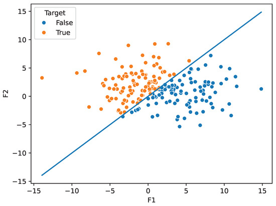
Figure 1.
Plot numerical order. displaying the dataset.
3.1.2. Trigonometric Dataset
The trigonometric dataset is a numeric dataset based on the sine function. It consists of two relevant, five redundant, and fifty irrelevant features, as well as 200 instances of data. We generated the relevant features, and , using normal distributions with N(2, 2) and N(−2, 1), respectively. We then divided the data points into two classes using the inequality (Figure 2).
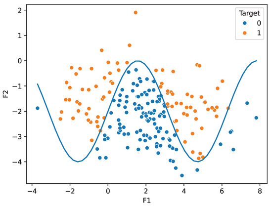
Figure 2.
Plot displaying the trigonometric dataset.
3.1.3. Hypersphere Dataset
The hypersphere dataset is a numeric dataset based on spheres. It consists of 3 relevant, 20 redundant, and 100 irrelevant features, for 400 instances of data. We generated and using exponential distributions with and , respectively, and using a gamma distribution with and . We then divided the data points into two classes using the inequality (Figure 3).
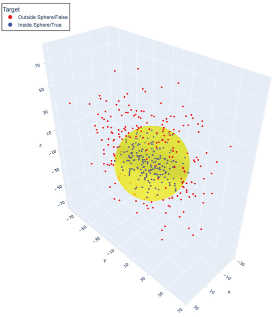
Figure 3.
Plot displaying the hypersphere dataset.
3.1.4. Cone Dataset
The cone dataset, similar to the hypersphere, is inspired by geometry. We used three relevant features, , , and , generated using three normal distributions, N(5, 9), N(0, 25), and N(10, 25). We then combined them with 20 redundant features and 100 irrelevant features. The classes were assigned using the equation: (Figure 4).
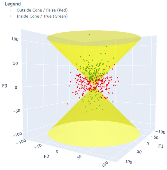
Figure 4.
Plot displaying the cone dataset.
3.1.5. Double Spiral Dataset
The double spiral dataset consists of data points found along one of two spirals drawn in three-dimensional space. The dataset consists of three relevant features used to generate 30 redundant features. Then, 120 irrelevant features were added to the dataset. Each of the three relevant features was generated using the following equations for each class, based on a continuous variable (Figure 5):
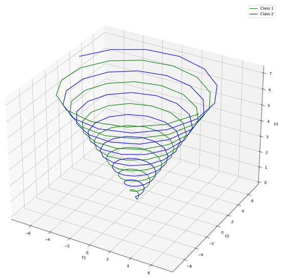
Figure 5.
Plot displaying the double spiral dataset.
Equation for Class 1:
Equation for Class 2:
3.1.6. Five-Class Multi-Cut Dataset
The multi-cut dataset is a numeric dataset with each data point belonging to one of five classes (Figure 6). It consists of 6 relevant, 20 redundant, and 100 irrelevant features for 500 instances of data points. We generated and using N(10, 5) and N(−10, 5), respectively; and using -distributions with = (10, .4) and = (15, .5), respectively; and and using exponential distributions with and , respectively. Based on the generated samples, we defined the following split equation in order to define the five classes of the target variable:
where f is an arbitrarily selected linear combination of the relevant features given by:
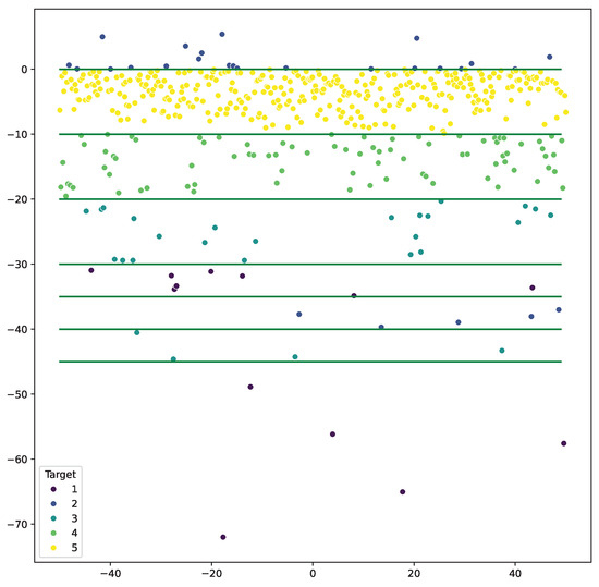
Figure 6.
Plot displaying the five-class multi-cut dataset.
3.1.7. Ten-Class Multi-Cut Dataset
This dataset is an extension of the five-class dataset with double the number of possible classes. It consists of 6 relevant, 20 redundant, and 100 irrelevant features for 500 instances of data. We generated and using N(10, 5) and N(−10, 5), and using -distributions with = (10, .4) and = (15, .5), and and using exponential distributions with and . Similar to the five-class dataset, we defined the following equation to define the ten classes of the target variable (Figure 7):
where .
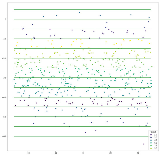
Figure 7.
Plot displaying the ten-class multi-cut dataset.
3.1.8. Yin–Yang Dataset
The image of the Chinese philosophical concept of Yin-Yang, depicted in Figure 8, inspired this dataset. To generate a dataset, we converted the pixels in an image of the Yin–Yang symbols into over a hundred thousand data points; the coordinates of each pixel are the relevant features, and the color defines the class of the binary target variable. As a result, we had two relevant features and added ten redundant and fifty irrelevant features. We scaled down the dataset to 600 instances.

Figure 8.
Plot displaying the Yin–Yang dataset.
3.1.9. 4D AND
The four-dimensional AND dataset is one that uses categorical data as its relevant features. We used four binary features, to , to generate eight redundant features using the NOT function. We then added 100 irrelevant features into the dataset. The relevant features were then used to split the dataset using the simple equation: (Figure 9).
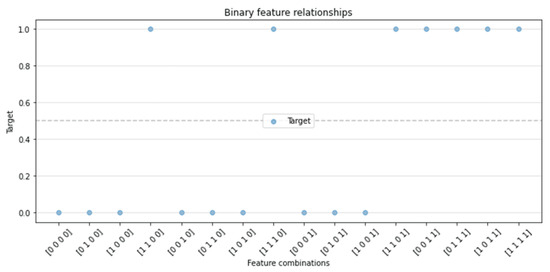
Figure 9.
Plot displaying the 4D AND dataset.
3.1.10. 5D XOR
The five-dimensional XOR dataset is very similar to the AND dataset. We used five binary features, ×1 to ×5, to generate ten redundant features using the NOT function. We then added 100 irrelevant features. We had a total of 100 instances, and the dataset was split using the XOR function as follows: (Figure 10).
Figure 10.
Plot displaying the 5D XOR dataset.
Table 1 provides a summary of our generated datasets.

Table 1.
Summary of datasets.
4. Methodology
In this study, we selected an array of FSAs and tested their performance on our synthetically generated datasets. Our tests involved running the algorithms on our datasets and tasking them to provide a number of features equal to the number of originally generated relevant features and then twice that number. Each time, we used the number of correct features selected as the performance metric. We defined a correct feature as either a relevant feature or a redundant feature of a relevant feature that had not been selected yet. If an algorithm selected two redundant features that were generated from the same relevant feature, then it counted as only one correct feature being selected.
Despite a wide variety of algorithms for feature selection, there is no agreed “best” algorithm, as FSAs are generally purpose-built for a specific application [24]. By this, we are referring to the fact that different FSAs work well on different data, depending on their size, type, and general application. One of the most popular feature selection algorithms that is well-tested within the field is Minimum Redundancy Maximum Relevance (mRMR) [35]. mRMR selects features based on calculations of which features correlate most with the target (relevance)—and which features correlate least with each other (redundancy) [36]. Both of these optimization criteria are used to develop the feature selection information. Other feature selection algorithms include decision tree entropy-based feature selection [37], Sequential Forward Selection (SFS) [38], and Sequential Backward Selection (SBS) [39].
4.1. Feature Selection Algorithm Testing
For this work, we used the following list of FSAs:
- Entropy—an algorithm that tries to maximize the information gained by selecting a certain feature with entropy as the measure of impurity [40].
- Gini Index (Gini)—similar to Entropy, this algorithm aims to maximize the information gain when selecting features but uses the Gini Index as its measure of impurity [41].
- Mutual Information (MI)—this algorithm uses the concept of mutual information, which measures the reduction in uncertainty for the target variable given the selection of a certain feature [41].
- Sequential Backward Selection (SBS)—this algorithm sequentially removes features until there is significant increase in the misclassification of a supporting classifier. We used a Support Vector Machine with an rbf kernel for our experiments [42].
- Sequential Forward Selection (SFS)—this algorithm is similar to SBS; however, it is the sequential adding of features until there is no significant decrease in the misclassifcation of a supporting classifier. We use a Support Vector Machine with an rbf kernel for our experiments [42].
- Symmetrical Uncertainty (SU)—uses the interaction of a feature with other features to determine which features are best [43].
- Minimum Redundancy Maximum Relevance (mRMR)—this algorithm is a minimal-optimal feature selection algorithm that sequentially selects the feature with maximum relevance to the target variable but also has the minimum redundancy when compared to the previously selected features [44].
- Genetic Feature Selection Algorithm (GFA)—a genetic algorithm inspired by the concepts of evolution and natural selection used from the sklearn-genetic library [45].
In the next section, the selected FASs are ranked and evaluated on their ability to identify the correct features in the generated datsets and also on their robustness or resilience to noise.
4.2. Complexity
When developing testing benchmarks for feature selection algorithms, an understanding of how difficult or complex the datasets used are is crucial. While designing and generating our synthetic datasets, we developed an understanding of how hard it would be for a feature selection algorithm to accurately pick out the relevant features. By using this information, we can measure the sophistication of feature selection algorithms based on how well they perform on datasets with different levels of complexity.
There is limited literature on a commonly agreed “difficulty” or “complexity” of synthetically generated datasets. Only a few papers such as [46,47] have attempted to define the complexity of a dataset. However, neither are regarded as the standard to measure complexity in the field. Hence, we propose groupings of complexity based merely on empirical results. To do so, we tested eight different FSAs on all the datasets and kept a record of the percentage of correct features identified across all datasets, where a correct feature is defined in the next Section 4. We used the distribution of the average percentage of identified correct features as the basis for grouping the datasets in terms of difficulty. A statistical test was applied to validate the groupings, where we expected datasets in each group to have a similar performance across the different FSAs.
4.3. Noise Resilience
Noise is a common feature of most datasets. As a result, research has been conducted into the handling of noise in all kinds of datasets and applications [48,49,50]. In this work, we explored the robustness of Feature Selection Algorithms through two kinds of noise: asymmetric label noise and irrelevant feature addition. Asymmetric label noise was created by selecting a random fraction of data points in the dataset and swapping their labels to the other class using fixed rules. For example, a point selected from the ith class would be converted to the (i + 1)th class in that dataset. Meanwhile, in our following experiments, we removed the irrelevant features from the dataset and then replaced these features while tracking the change in the FSA performance. Other methods of adding noise exist in the literature, like the addition of Gaussian noise to the data samples. We decided to limit ourselves to two methods of noise addition as it seemed sufficient for the scope of this work. Below is the summary of our noise addition methods:
- Class Changing: Randomly change the target variable classes to different classes for a subset of data.
- Reducing the number of irrelevant features: Randomly dropping a subset of irrelevant variables from the generated data, i.e., reducing the level of noise in the dataset.
For each of the two noise addition methods, we varied the size of the subset of the data to which noise was added by varying a percentage of the classes of the instances (or number of irrelevant features, respectively), between 0% and 50%. As the level of noise moves from 0% to 50% for class changing, the level of noise increases. Furthermore, the level of noise increases, as the percentage of the removed irrelevant features decreases from 50% to 0%.
5. Results
In this section, we present the results of the evaluation of the performance of the selected FSAs on our generated datasets. We begin first by counting the number of correct features identified by each algorithm for each dataset. We use the results to group the datasets in terms of complexity and examine the performance of each FSA across the different complexity groups. Further evaluation of the FSA performance was conducted by adding the two kinds of noise to the datasets, and we examine the percentage of correct features identified as the level of noise increases.
5.1. Number of Correct Features Identified Per Dataset
We examine the number of correct features identified per dataset when selecting the number of features as the actual number of relevant features (as in Table 1) and twice the actual number of relevant features. Since a full length discussion of each FSA’s results on each of the datasets would be too long and derail us from the main purpose of the paper, we have included the entire discussion in Appendix A.
In the first round of experiments, we see that the SBS and SFS were the top performing FSAs on average. The SBS was able to identify all the relevant features for six out of ten of our datasets, and the SFS was able to do the same for five. Similar results were achieved when the FSAs were tasked with finding twice the number of relevant features. On the other hand, we see that the GFA and Gini performed the worst, with each only once finding all the relevant features of a dataset when tasked with finding twice the number of relevant features. The average fraction of correct features selected by each algorithm is summarized in Table 2. This average is calculated using the results reported in Appendix A for each dataset.
Table 2.
Average and standard deviation of the FSA performance across datasets, for feature subset size equal to the number of relevant features and twice the number of relevant features from the datasets. Green represents cases where over of the correct features were chosen, and red represents cases where under of correct features were chosen.
When it comes to the datasets, we see that the FSAs often did well on the Straight line, Yin–Yang, and 4D AND datasets. At the same time, most of the FSAs failed to identify even one of the relevant features in the 5D XOR and the Double spiral datasets with the exception of the MI algorithm, which was able to identify one correct feature in the Double spiral dataset when selecting the feature subset size equal to the number of relevant features and twice the number of relevant features. Furthermore, the Entropy algorithm was able to find one of the relevant features when tasked with finding twice the number of relevant features in the 5D XOR dataset. The average performance of all the FSAs is given in Table 3 for each of the datasets.
Table 3.
Average and standard deviation of the FSA performance per dataset, for feature subset size equal to the number of relevant features and twice the number of relevant features from the datasets. Green represents cases where over of the correct features were chosen, and red represents cases where under of correct features were chosen.
5.2. Groupings of the Generated Datasets
As discussed in Section 4.2 above, we used the empirical results to construct groupings of the datasets. As observed in Figure 11, we see that the 4D AND and Straight line datasets had the best performance, while the 5D XOR and Double spiral datasets showed the worst performance. Figure 11 also suggests that the Yin–Yang dataset can be placed in the top level group; however, based on Figure 12 we see that the Yin–Yang dataset can be placed in a higher level of complexity when selecting twice the number of relevant features.
Figure 11.
The bar chart shows the average performance of the feature selection algorithms per dataset. Bars sharing the same color are in the same complexity grouping.
Figure 12.
The bar chart shows the average performance of the feature selection algorithms per dataset when looking for 2× # of relevant features. Bars sharing the same color are in the same complexity grouping.
Using both set of results, we conducted a series of Kruskal–Wallis tests to compare the set of results for each dataset. We conducted the test comparing the average fraction of correct features identified per dataset in each possible grouping of neighbors in Figure 11. We concluded the final groups when the Kruskal–Wallis test within the group showed no statistical difference but the test between the consecutive groups showed a statistically significant difference. These tests show that the four most complex datasets are actually statistically significantly different. As a result, we decided to use these four complexity groups:
- Group 1—Low Complexity: Straight line (), 4D AND;
- Group 2—Medium Complexity: Yin–Yang, Trigonometric, Hypersphere, Cone;
- Group 3—High Complexity: Ten-class multi-cut, Five-class multi-cut;
- Group 4—Very High Complexity: Double spiral, 5D XOR.
In the next section, we evaluate the noise resilience of the eight FSAs considering the complexity groupings identified above.
5.3. Noise Resilience of the FSAs
Now that we have tested several FSAs on the proposed datasets and provided a comprehensive ranking of the datasets in terms of the FSAs’ performance, we now examine the resilience of different FSAs to noisy data. We explore the two methods of adding noise to the datasets described in Section 4.3 in order to to examine the stability and resilience to noise of the FSA.
Note: Some of the figures in this section have overlapping lines. As a way to combat that, we added small lines around the markers on the graph to indicate what other markers (of the same color) are hidden behind this line. A combination of the visible markers and these lines should be able to give any reader a complete understanding of our results.
5.3.1. Class-Wise Noise
- Group 1—Low Complexity
Figure 13 depicts the average percentage of correct features identified across the complexity group 1 datasets for varying ratios of induced class flip noise when selecting a feature subset of a size equal to the number of relevant features (a) and twice the number of relevant features (b).
Figure 13.
Class flip noise results for all feature selection algorithms across the group 1 datasets. (a) Class flip noise results selecting the actual number of relevant features; (b) class flip noise results selecting twice the actual number of relevant features.
Most FSAs experienced a sharp decline in performance when 30% or more of the classes were changed as shown in Figure 13a. Most FSAs had a stable performance when less than 20% of the classes were changed, indicating a limited robustness to mislabelled data for the easy datasets. A similar trend is observed when twice the number of features were chosen as shown in Figure 13b, but a few algorithms performed slightly better on average, such as the SBS, Symmetric uncertainty, mRMR, and Entropy. We also notice that in general most algorithms performed the same or slightly better when selecting twice the number of relevant features.
- Group 2—Medium Complexity
Figure 14 shows the average percentage of correct features identified across the complexity group 2 datasets.
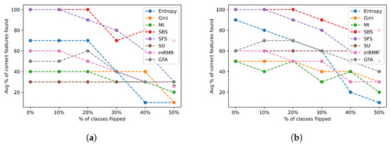
Figure 14.
Class flip noise results for all feature selection algorithms across group 2 datasets. (a) Class flip noise results selecting the actual number of relevant features; (b) class flip noise results selecting twice the actual number of relevant features.
FSAs in this group have a much more stable performance and resilience to mislabelled data, as illustrated in Figure 14a,b. In particular, almost all the FSAs obtained a stable performance with up to 20% of the classes changed, as shown in Figure 14a, with SU achieving a stable performance even with over half the classes changed. However, this performance was relatively poor. In contrast, SBS maintained a relatively stable and highly accurate performance regardless of the number of features it was asked to select. In general, we observe an obvious trend in which most of the FSAs performed better when allowed to select a larger subset of features, as shown in Figure 14b.
- Group 3—High Complexity
Figure 15 shows the average percentage of correct features identified across complexity group 3 datasets.
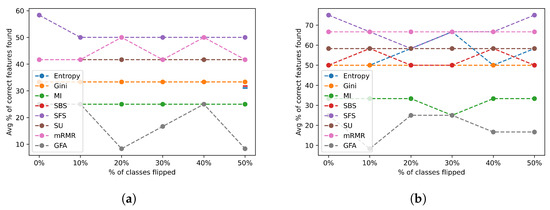
Figure 15.
Class flip noise results for all feature selection algorithms across group 3 datasets. (a) Class flip noise results selecting the actual number of relevant features; (b) class flip noise results selecting twice the actual number of relevant features.
As shown in both Figure 15a,b above, almost every FSA consistently performed the same regardless of the level of noise. Similar to group 2, Figure 15b shows a higher average performance than Figure 15a. As expected, none of the algorithms performed with over 75% accuracy, since this is the hard group of datasets. However, most algorithms were very stable but were unable to achieve over 50% accuracy when tasked with selecting fewer features. This indeed emphasizes the importance of determining the number of features to be selected, especially for a considerable level of data complexity. As seen in Figure 15b, only five FSAs were able to achieve 50% accuracy or higher. Moreover, a notable observation is that the GFA and MI failed harshly in this category identifying less than 30% of the features correctly on average. Hence, the GFA and MI are unsuitable to use for a dataset with complex decision boundaries.
- Group 4—Very High Complexity
Figure 16 shows the average percentage of correct features identified across complexity group 4 datasets.
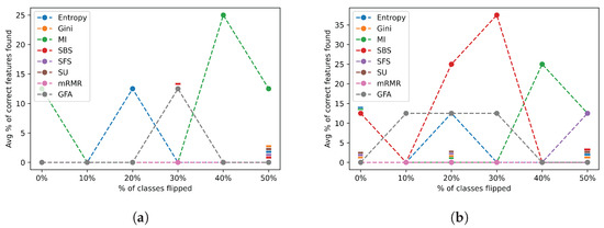
Figure 16.
Class flip noise results for all feature selection algorithms across group 4 datasets. (a) Class flip noise results selecting the actual number of relevant features; (b) class flip noise results selecting twice the actual number of relevant features.
As shown in Figure 16a,b, almost every FSA consistently performed very poorly, with most FSAs consistently not finding any features, as shown in Figure 16a. The MI, Entropy, and SBS managed to identify some of the relevant features but still eventually failed even at very low noise levels. The SBS ultimately performed the best when selecting a higher number of features (as in Figure 16b) but still achieved a maximum of below 40% accuracy. However, due to the erratic behavior of these FSAs and most of them identifying little to no correct features at 0% noise levels, we can conclude that any improvements seen here are merely coincidental or due to the random noise. Hence, the final group with the highest difficulty led to most FSAs failing completely when any mislabelled data were presented.
Table 4 and Table 5 below exhibit the average performance of each FSA across all noise levels and all datasets in each complexity group. The two tables provide the average and standard deviation values for the number of correct features identified when the size of the selected feature subset is equal to the number of relevant features (Table 4) and twice the relevant features (Table 5).
Table 4.
The average and standard deviation of the correct number of features identified across all noise levels by each FSA for selecting 1× the number of relevant features. Green represents cases where over of the correct features were chosen, and red represents cases where under of correct features were chosen.
Table 5.
The average and standard deviation of the correct number of features identified across all noise levels by each FSA for selecting 2× the number of relevant features. Green represents cases where over of the correct features were chosen, and red represents cases where under of correct features were chosen.
A well-performing FSA is has a high average and low standard deviation indicating high accuracy and high stability. As expected, all the algorithms performed better or equally well when selecting a higher number of features, as the performance of the FSAs in each group shown in Table 5 was better than their performance shown in Table 4. Furthermore, as the data complexity level increases, the FSAs suffer from reduced accuracy with increased stability.
From the above analysis, we can identify the best performing algorithm for each data complexity group:
- Group 1—Low Complexity: SBS;
- Group 2—Medium Complexity: SBS;
- Group 3—High Complexity: SFS;
- Group 4—Very High Complexity: MI.
It is worth noting that group 4 has MI as the most accurate algorithm; however, it is also the most unstable algorithm in Table 4. Moreover, the SBS may seem like the most accurate algorithm when selecting more features, as shown in Table 5; however, it has an extremely large standard deviation, making it very unstable.
All Datasets
A further examination of the trends across all the datasets presented in Figure A1a,b (Appendix A) and the last column in Table 4 and Table 5 above reveals the following main takeaways:
- There is no significant degradation in the performance of the FSAs when up to 20% of the class labels are changed. This observation holds true when selecting both the actual number of relevant features and twice the number of relevant features. This suggests that the additional features found were often not relevant when there were mislabelled data.
5.3.2. Irrelevant Feature Noise
- Group 1—Low Complexity
Figure 17 depicts the average percentage of correct features identified for the datasets in complexity group 1 for varying ratios of removed irrelevant features when selecting the actual number of relevant features (a) and twice the number of relevant features (b).
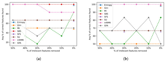
Figure 17.
Noise results for irrelevant features across group 1 datasets. (a) Irrelevant feature noise results selecting the actual number of relevant features; (b) irrelevant feature noise results selecting twice the actual number of relevant features.
Most FSAs are easily able to consistently find all the relevant features, as shown in Figure 17a,b. This is demonstrated by the straight line at 100% of the correct features found in both figures for some FSAs. However, there are a few FSAs that performed poorly, such as the Gini, GFA, and MI that identified less than 50% of the correct features. Generally speaking, most algorithms continued to maintain their performance, while others improved their accuracy when selecting a higher number of features, as shown in Figure 17b.
- Group 2—Medium Complexity
Figure 18 depicts the average percentage of correct features identified for the datasets in complexity group 2 for varying ratios of removed irrelevant features when selecting the actual number of relevant features (a) and twice the number of relevant features (b).
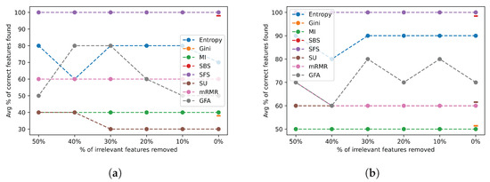
Figure 18.
Noise results for Irrelevant features across group 2 datasets. (a) Irrelevant feature noise results selecting the actual number of relevant features; (b) irrelevant feature noise results selecting twice the actual number of relevant features.
As seen in Figure 17, the FSAs have a consistent performance with group 2 datasets too. There are slight differences in performance between the group 1 datasets and the group 2 datasets. This is expected to a certain extent since most popular FSAs are generally robust to the number of irrelevant features in the dataset. Further, Figure 18 exhibits a clear improved performance of all FSAs when twice the number of relevant features are identified.
- Group 3—High Complexity
The results for the group 3 datasets are displayed in Figure 19.
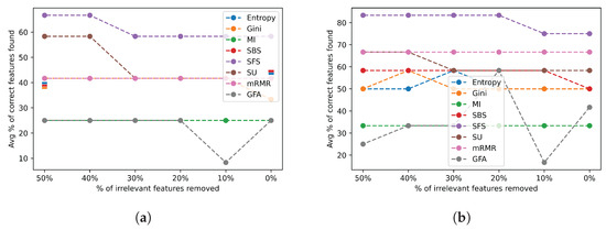
Figure 19.
Noise results for irrelevant features across group 3 datasets. (a) Irrelevant feature noise results selecting the actual number of relevant features; (b) irrelevant feature noise results selecting twice the actual number of relevant features.
On average, many FSAs continued to maintain consistent performance showing a great level of resilience to additional irrelevant features, even for harder datasets. However, this performance is less than that seen for the datasets in groups 1 and 2. Hence, even though the graphs in Figure 19a,b show some consistent performances, the average number of features identified have dropped significantly in comparison to easier groups.
- Group 4—Very High Complexity
Figure 20 shows the average percentage of correct features identified for the very high complex datasets.
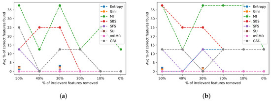
Figure 20.
Class flip noise results for irrelevant features across group 4 datasets. (a) Irrelevant feature noise results selecting the actual number of relevant features; (b) irrelevant feature noise results selecting twice the actual number of relevant features.
Figure 20a,b show the poor performance most FSAs have on the datasets in group 4, with the majority of them consistently achieving an accuracy of 0% or near. The best FSAs—MI and SBS—also fail to exceed 35% accuracy and have a relatively erratic behavior, which is very unusual compared to their performance for the datasets in groups 1, 2, and 3. This further illustrates how these datasets in group 4 make it difficult for FSAs to identify the correct features. In addition, none of the FSAs is able to achieve a major improvement when selecting a higher number of features.
Table 6.
The average and standard deviation of the correct number of features identified across all noise levels by each FSA for the number of relevant features. Green represents cases where over of the correct features were chosen, and red represents cases where under of correct features were chosen.
Table 7.
The average and standard deviation of the correct number of features identified across all noise levels by each FSA for 2× the number of relevant features. Green represents cases where over of the correct features were chosen, and red represents cases where under of correct features were chosen.
As expected, all algorithms perform better or equally well when selecting a larger number of features. The performance of the FSAs in each group shown in Table 7 is generally better than their performance shown in Table 6. As illustrated in Section 5.3.1, a desired FSA is the the one with high average and low standard deviations, which indicate high accuracy and high stability. Similar to the trend observed in Table 4 and Table 5, the more complex a dataset is, the less accurate the FSAs are in identifying the correct features. Furthermore, Table 6 and Table 7 show that the majority of the FSAs suffered from high standard deviations relative to the average performance in the group 4 datasets. These FSAs are not of much use in this case.
Based on the resilience of FSAs to irrelevant features-related noise, we can conclude the best performing algorithm for each difficulty group:
- Group 1—Low Complexity: SBS;
- Group 2—Medium Complexity: SBS and SFS;
- Group 3—High Complexity: SFS;
- Group 4—Very High Complexity: MI.
It is worth noting that the stability of several FSAs was unaffected by the number of features selected, showing that the algorithms are extremely stable in regard to the number of irrelevant features being used, as expected of an FSA.
All Datasets
A further examination of the trends across all datasets presented in Figure A2a,b (Appendix A) and the last column in Table 6 and Table 7 above reveals that, on average, most FSAs were relatively stable when dealing with noise based on the number of irrelevant features as would be expected. Most FSAs show consistent performance across every noise level but with a higher overall performance when selecting a larger number of features.
5.3.3. Discussion
Comparing the overall performance of Figure A1 and Figure A2, we see that on average, FSAs are able to identify fewer relevant features when the noise is based on the class being mislabelled than when the noise relates to the number of irrelevant features in the datasets. This is numerically seen where the highest percentage of correct features found across all datasets when altering the target variable is 60–70% depending on the number of selected features, while the lowest percentage of correct features found is 10–20%. However, the highest percentage of correct features found when the noise is based on irrelevant features is 70–80% and the lowest percentage is 20–40%. This illustrates how the irrelevant features did not affect the performance of the FSAs as much as the class changing, as expected. This can be graphically seen since Figure A2 has more straight lines showing consistent performance across different levels of noise, but there is a lack of horizontal lines in Figure A1.
This is expected since most FSAs are built to deal with a varying number of irrelevant features to begin with and, hence, are more resilient to that kind of noise. On the other hand, most FSAs are highly reliant on the distribution of the data with respect to the target variable, which is what changes when we add noise through changing the classes. This shows that most FSAs are not resilient to mislabelled data but highly resilient to additional irrelevant features.
The analysis conducted in this section is an example of how one can evaluate their own feature selection algorithm using the provided datasets. Following the analysis in this work, users of the feature selection process can draw valuable insights into the performance, points of failure, resilience to noise, and stability of the FSAs of interests. In addition to providing details about a particular FSA, this can allow a standardized form of FSA comparison that can be used to benchmark an FSA against other popular or newly developed FSAs.
Our aim of this analysis is to have it serve as a stepping stone to more a comprehensive but standardized analysis and comparison of FSAs. Further guidance on how the reader can use the datasets for their own analysis is provided in the following section.
6. How to Use Our Datasets
In this section, we give a concise and easy-to-follow guide on how to test new FSAs not included in this paper. All the datasets presented in this paper are available at our Github repository (https://github.com/ro1406/SynthSelect, accessed on 24 January 2024), with some helper functions to load them, as well as to adjust the number of redundant and irrelevant features for both numeric and categorical datasets. The latter mentioned functions can be used to conduct independent testing and allow developers to create their own datasets. However, we recommend using the datasets presented here to allow for standardized bench-marking of FSAs in the community.
6.1. Basic Test
These are the steps to test the basic performance of an FSA algorithm. Repeating the following steps multiple times is recommended to account for the variation in FSA performance. The results across datasets can also be aggregated within complexity levels for better comparison to the previously tested algorithms.
- Run the selected FSA on each dataset within a group, setting it so that the FSA must return features equal to the number of relevant features for each dataset.
- The score of any FSA would be the precentage of relevant/non-repeated redundant features correctly selected.
- It is important to note that FSAs might break and report the first n columns. It is a good idea to shuffle the arrangement of the columns during testing.
- Repeat with the FSA set to return a number of features equal to double the number of relevant features for each dataset.
6.2. Stability Test
After testing the basic performance of an FSA, one can test how stable the algorithm is. To do this, one can follow the following steps:
- Begin by selecting either the Class flip or Irrelevant feature noise. Code is provided in this Github (https://github.com/ro1406/SynthSelect, accessed on 24 January 2024).
- For each level of noise, move through the same steps listed in Section 6.1 using the newly formed dataset.
- Report the score across all noise levels and groups to have a suitable metric to compare to previously tested FSAs.
7. Conclusions
In this paper, we have presented the synthetic generation of ten separate datasets that were tested using eight feature selection algorithms. These generated datasets were designed specifically for the purposes of re-usability by researchers and for the evaluation of relevant feature selection algorithms. By conducting the experiments shown in this work, we have confirmed the promise of using synthetic datasets for determining the performance of FSAs. By allowing researchers to experiment with the specific details of datasets, such as the number of relevant, irrelevant, or redundant features, target variables, and beyond, we are able to grasp a stronger sense of any FSA’s performance. Additionally, the existence of such synthetic data and their generation allows for the development of novel feature selection techniques and algoithms. The datasets generated are provided to readers through our GitHub repository, as explained in Section 6. Researchers are encouraged to adjust the datasets according to their specific criteria. For future work, we recommend researchers continue working with the generation of datasets other than numerical, such as categorical and ordinal data. More specifically, we recommend the generation of synthetic data pertaining to time series and regression problems. This allows for further testing and evaluation of feature selection algorithms for a broader scope in the field.
Author Contributions
Conceptualization, F.K. and H.S.; methodology, R.M., E.A., D.V., H.S. and F.K.; software, R.M., E.A. and D.V.; validation, R.M., E.A. and D.V.; formal analysis, F.K., H.S., R.M., D.V. and E.A.; investigation, R.M., E.A. and D.V.; resources, R.M., E.A., D.V. and H.S.; data curation, R.M. and E.A.; writing—original draft preparation, R.M., E.A. and D.V.; writing—review and editing, H.S. and F.K.; visualization, R.M. and F.K.; supervision, H.S., F.K. and R.M.; project administration, H.S.; funding acquisition, H.S. All authors have read and agreed to the published version of the manuscript.
Funding
This research was supported, in part, by the Open Access Program from the American University of Sharjah.
Data Availability Statement
The datasets used in this study can be found at the mentioned GitHub repository (https://github.com/ro1406/SynthSelect, accessed on 24 January 2024).
Conflicts of Interest
The authors declare no conflict of interest.
Appendix A
Table A1.
4D AND.
Table A1.
4D AND.
| Algorithm | Real_Feat | 2 × Real_Feat |
|---|---|---|
| Entropy | 4 | 4 |
| GFA | 0 | 3 |
| Gini | 2 | 3 |
| MI | 4 | 4 |
| mRMR | 4 | 4 |
| SBS | 4 | 4 |
| SFS | 2 | 2 |
| SU | 2 | 3 |
The majority of the FSAs found the four correct features for the 4D AND dataset, with the other FSAs finding two and three features, respectively. This shows that it is relatively easy to identify the important features in this dataset. However, the genetic feature selection algorithm was unable to find any correct features initially but found three out of the five correct features when made to choose its top eight features. This can be explained due to the stochastic nature of feature selection algorithms. Since genetic feature selection algorithms rely on random initialization, it is possible that we do not obtain the relevant features in some cases. However, increasing the top features to twice its initial implementation increases the likelihood of finding them.
Table A2.
5D XOR.
Table A2.
5D XOR.
| Algorithm | Real_Feat | 2 × Real_Feat |
|---|---|---|
| Entropy | 0 | 1 |
| GFA | 0 | 0 |
| Gini | 0 | 0 |
| MI | 0 | 0 |
| mRMR | 0 | 0 |
| SBS | 0 | 0 |
| SFS | 0 | 0 |
| SU | 0 | 0 |
A similar trend can be seen for the Straight line dataset where all FSAs except for Mutual Information were able to find both correct features regardless of the number of features chosen. Mutual Information, however, was only able to find one correct feature even when the number of selected features was four.
Table A3.
.
Table A3.
.
| Algorithm | Real_Feat | 2 × Real_Feat |
|---|---|---|
| Entropy | 2 | 2 |
| GFA | 1 | 2 |
| Gini | 1 | 1 |
| MI | 1 | 1 |
| mRMR | 2 | 2 |
| SBS | 2 | 2 |
| SFS | 2 | 2 |
| SU | 2 | 2 |
However, a drastically different trend can be seen for the nonlinearly separable categorical XOR dataset, where none of the FSAs were able to find even a single correct feature out of the five possible correct features. Only Entropy was able to find a single correct feature when asked to select the top 10 features. Since none of the FSAs found even a single correct feature, they found the irrelevant features to be more useful in determining the final class.
Table A4.
Cone.
Table A4.
Cone.
| Algorithm | Real_Feat | 2 × Real_Feat |
|---|---|---|
| Entropy | 2 | 2 |
| GFA | 2 | 2 |
| Gini | 1 | 1 |
| MI | 1 | 1 |
| mRMR | 1 | 1 |
| SBS | 3 | 3 |
| SFS | 3 | 3 |
| SU | 1 | 3 |
In terms of the Cone dataset, only the SFS and SBS found all three correct features each time, and the SU identified only one correct feature at first but then found all three when asked to pick the top six features. Entropy also consistently found two out of three features. However, the other three algorithms only found one feature each time despite the decision boundary not being very complicated.
Table A5.
Double spiral.
Table A5.
Double spiral.
| Algorithm | Real_Feat | 2 × Real_Feat |
|---|---|---|
| Entropy | 0 | 0 |
| GFA | 0 | 0 |
| Gini | 0 | 0 |
| MI | 1 | 1 |
| mRMR | 0 | 0 |
| SBS | 0 | 1 |
| SFS | 0 | 0 |
| SU | 0 | 0 |
Lastly, only the MI was consistently able to identify only one of the three correct features in the Double spiral dataset, with none of the other FSAs identifying even one of the correct features. The SBS, however, did manage to find one correct feature when selecting the top six features.
Table A6.
Hypersphere.
Table A6.
Hypersphere.
| Algorithm | Real_Feat | 2 × Real_Feat |
|---|---|---|
| Entropy | 2 | 3 |
| GFA | 1 | 2 |
| Gini | 1 | 1 |
| MI | 1 | 1 |
| mRMR | 2 | 2 |
| SBS | 3 | 3 |
| SFS | 3 | 3 |
| SU | 1 | 2 |
A similar trend holds true for the Hypersphere dataset where the SBS and SFS find all the correct features consistently; the SU only finds one initially and eventually finds two correct features. However, this time only the Gini and MI were unable to find the majority of the correct features even when selecting the top six features for the dataset. Together, the Cone and Hypersphere datasets indicate how the Gini and MI fail to perform well on curved surface decision boundaries in higher dimensions.
Table A7.
Trigonometric.
Table A7.
Trigonometric.
| Algorithm | Real_Feat | 2 × Real_Feat |
|---|---|---|
| Entropy | 1 | 2 |
| GFA | 1 | 1 |
| Gini | 1 | 2 |
| MI | 1 | 2 |
| mRMR | 1 | 1 |
| SBS | 2 | 2 |
| SFS | 2 | 2 |
| SU | 1 | 1 |
Moreover, the Trigonometric dataset has all FSAs finding at least one out of the two correct features, with the SBS and SFS performing the best consistently and the Entropy, Gini, and MI finding the correct features when selecting the top four features.
Table A8.
Five-class multi-cut.
Table A8.
Five-class multi-cut.
| Algorithm | Real_Feat | 2 × Real_Feat |
|---|---|---|
| Entropy | 2 | 3 |
| GFA | 2 | 1 |
| Gini | 2 | 3 |
| MI | 2 | 2 |
| mRMR | 2 | 4 |
| SBS | 1 | 2 |
| SFS | 2 | 4 |
| SU | 3 | 4 |
The five-class multi-cut dataset has six correct features, which none of the algorithms found. The most correct features found was four, by the mRMR, SFS, and SU, all when choosing the top 12 features only. This shows how difficult this dataset is for feature selection algorithms when the data in the same class are disjoint. Most FSAs found two of six features easily but failed to make any major progress toward finding all six.
Table A9.
Ten-class multi-cut.
Table A9.
Ten-class multi-cut.
| Algorithm | Real_Feat | 2 × Real_Feat |
|---|---|---|
| Entropy | 3 | 3 |
| GFA | 1 | 2 |
| Gini | 2 | 3 |
| MI | 1 | 2 |
| mRMR | 3 | 4 |
| SBS | 4 | 4 |
| SFS | 5 | 5 |
| SU | 2 | 3 |
The Ten-class multi-cut dataset also has no FSA that could find all six features; however, the SFS came the closest, finding five of the six correct features consistently. SBS also performed well and much better than the in the Five-class multi-cut dataset consistently finding four out of six correct features. In fact, every FSA except for the SU performed better on the Ten-class multi-cut dataset than the Five-class multi-cut dataset. This is an interesting finding that needs to be explored.
Table A10.
Yin–Yang.
Table A10.
Yin–Yang.
| Algorithm | Real_Feat | 2 × Real_Feat |
|---|---|---|
| Entropy | 2 | 2 |
| GFA | 1 | 1 |
| Gini | 1 | 1 |
| MI | 1 | 1 |
| mRMR | 2 | 2 |
| SBS | 2 | 2 |
| SFS | 2 | 2 |
| SU | 0 | 0 |
The majority of the FSAs identified both of the correct features consistently, while the Gini and MI only found one out of the two correct features even when picking the top four features. However, the SU was consistently the poorest performer being unable to identify any of the correct features.
Below are the results of the noise testing of each FSA across all datasets.
Figure A1 contains the trends for the FSAs’ performances across all datasets for the various noise levels with class-wise noise.
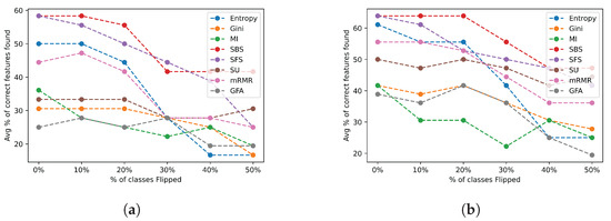
Figure A1.
Class flip noise results for all feature selection algorithms across all datasets. (a) Class flip noise results selecting the actual number of relevant features; (b) class flip noise results selecting twice the actual number of relevant features.
Figure A2 contains the trends for the FSAs’ performances across all datasets for the various noise levels with irrelevant feature-based noise.
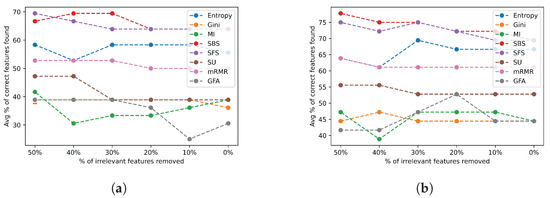
Figure A2.
Noise results for irrelevant features across all datasets. (a) Irrelevant feature noise results selecting the actual number of relevant features; (b) irrelevant feature noise results selecting twice the actual number of relevant features.
References
- Bolón-Canedo, V.; Sánchez-Maroño, N.; Alonso-Betanzos, A. An ensemble of filters and classifiers for microarray data classification. Pattern Recognit. 2012, 45, 531–539. [Google Scholar] [CrossRef]
- Shilaskar, S.; Ghatol, A. Feature selection for medical diagnosis: Evaluation for cardiovascular diseases. Expert Syst. Appl. 2013, 40, 4146–4153. [Google Scholar] [CrossRef]
- Feng, Y.; Akiyama, H.; Lu, L.; Sakurai, K. Feature Selection for Machine Learning-Based Early Detection of Distributed Cyber Attacks. In Proceedings of the 2018 IEEE 16th Intl Conf on Dependable, Autonomic and Secure Computing, 16th Intl Conf on Pervasive Intelligence and Computing, 4th Intl Conf on Big Data Intelligence and Computing and Cyber Science and Technology Congress(DASC/PiCom/DataCom/CyberSciTech), Athens, Greece, 12–15 August 2018; pp. 173–180. [Google Scholar] [CrossRef]
- Sulieman, H.; Alzaatreh, A. A Supervised Feature Selection Approach Based on Global Sensitivity. Arch. Data Sci. Ser. (Online First) 2018, 5, 3. [Google Scholar]
- Pudjihartono, N.; Fadason, T.; Kempa-Liehr, A.W.; O’Sullivan, J.M. A Review of Feature Selection Methods for Machine Learning-Based Disease Risk Prediction. Front. Bioinform. 2022, 2, 927312. [Google Scholar] [CrossRef]
- Mitra, R.; Varam, D.; Ali, E.; Sulieman, H.; Kamalov, F. Development of Synthetic Data Benchmarks for Evaluating Feature Selection Algorithms. In Proceedings of the 2022 2nd International Seminar on Machine Learning, Optimization, and Data Science (ISMODE), Virtual, 22–23 December 2022; pp. 47–52. [Google Scholar] [CrossRef]
- Friedman, J.H. Multivariate Adaptive Regression Splines. Ann. Stat. 1991, 19, 1–67. [Google Scholar] [CrossRef]
- Breiman, L. Bagging predictors. Mach. Learn. 1996, 24, 123–140. [Google Scholar] [CrossRef]
- Kao, L.J.; Chiu, C.C. Application of integrated recurrent neural network with multivariate adaptive regression splines on SPC-EPC process. J. Manuf. Syst. 2020, 57, 109–118. [Google Scholar] [CrossRef]
- Yamada, Y.; Lindenbaum, O.; Negahban, S.; Kluger, Y. Deep supervised feature selection using Stochastic Gates. arXiv 2018, arXiv:1810.04247. [Google Scholar]
- Yu, K.; Yang, Y.; Ding, W. Causal Feature Selection with Missing Data. ACM Trans. Knowl. Discov. Data 2022, 16, 1–24. [Google Scholar] [CrossRef]
- Alkhalifah, T.; Wang, H.; Ovcharenko, O. MLReal: Bridging the gap between training on synthetic data and real data applications in machine learning. arXiv 2021, arXiv:2109.05294. [Google Scholar] [CrossRef]
- Panday, D.; Cordeiro de Amorim, R.; Lane, P. Feature weighting as a tool for unsupervised feature selection. Inf. Process. Lett. 2018, 129, 44–52. [Google Scholar] [CrossRef]
- Kaya, S.K.; Navarro-Arribas, G.; Torra, V. Dynamic Features Spaces and Machine Learning: Open Problems and Synthetic Data Sets. In Integrated Uncertainty in Knowledge Modelling and Decision Making; Huynh, V.N., Entani, T., Jeenanunta, C., Inuiguchi, M., Yenradee, P., Eds.; Springer: Cham, Switzerland, 2020; pp. 125–136. [Google Scholar]
- Rughetti, D.; Sanzo, P.D.; Ciciani, B.; Quaglia, F. Dynamic Feature Selection for Machine-Learning Based Concurrency Regulation in STM. In Proceedings of the 2014 22nd Euromicro International Conference on Parallel, Distributed, and Network-Based Processing, Torino, Italy, 12–14 February 2014; pp. 68–75. [Google Scholar] [CrossRef]
- Yu, K.; Guo, X.; Liu, L.; Li, J.; Wang, H.; Ling, Z.; Wu, X. Causality-based Feature Selection: Methods and Evaluations. arXiv 2019, arXiv:1911.07147. [Google Scholar] [CrossRef]
- Kamalov, F.; Sulieman, H.; Cherukuri, A.K. Synthetic Data for Feature Selection. arXiv 2022, arXiv:2211.03035. [Google Scholar] [CrossRef]
- John, G.H.; Kohavi, R.; Pfleger, K. Irrelevant Features and the Subset Selection Problem. In Machine Learning Proceedings 1994; Cohen, W.W., Hirsh, H., Eds.; Morgan Kaufmann: San Francisco, CA, USA, 1994; pp. 121–129. [Google Scholar] [CrossRef]
- Kim, G.; Kim, Y.; Lim, H.; Kim, H. An MLP-based feature subset selection for HIV-1 protease cleavage site analysis. Artif. Intell. Med. 2010, 48, 83–89. [Google Scholar] [CrossRef] [PubMed]
- Zhu, Z.; Ong, Y.S.; Zurada, J.M. Identification of Full and Partial Class Relevant Genes. IEEE/ACM Trans. Comput. Biol. Bioinform. 2010, 7, 263–277. [Google Scholar] [CrossRef] [PubMed]
- Liu, X.Y.; Liang, Y.; Wang, S.; Yang, Z.Y.; Ye, H.S. A Hybrid Genetic Algorithm with Wrapper-Embedded Approaches for Feature Selection. IEEE Access 2018, 6, 22863–22874. [Google Scholar] [CrossRef]
- Zhu, Z.; Ong, Y.S.; Dash, M. Wrapper–Filter Feature Selection Algorithm Using a Memetic Framework. IEEE Trans. Syst. Man Cybern. Part B (Cybern.) 2007, 37, 70–76. [Google Scholar] [CrossRef] [PubMed]
- Breiman, L.; Friedman, J.H.; Olshen, R.A.; Stone, C.J. Classification and Regression Trees; Wadsworth International Group: Belmont, CA, USA, 1984. [Google Scholar]
- Bolón-Canedo, V.; Sánchez-Maroño, N.; Alonso-Betanzos, A. A review of feature selection methods on synthetic data. Knowl. Inf. Syst. 2012, 34, 483–519. [Google Scholar] [CrossRef]
- Guyon, I.; Li, J.; Mader, T.; Pletscher, P.A.; Schneider, G.; Uhr, M. Competitive baseline methods set new standards for the NIPS 2003 feature selection benchmark. Pattern Recognit. Lett. 2007, 28, 1438–1444. [Google Scholar] [CrossRef]
- Wang, D.; Nie, F.; Huang, H. Feature Selection via Global Redundancy Minimization. IEEE Trans. Knowl. Data Eng. 2015, 27, 2743–2755. [Google Scholar] [CrossRef]
- Figueira, A.; Vaz, B. Survey on Synthetic Data Generation, Evaluation Methods and GANs. Mathematics 2022, 10, 2733. [Google Scholar] [CrossRef]
- Varol, G.; Romero, J.; Martin, X.; Mahmood, N.; Black, M.J.; Laptev, I.; Schmid, C. Learning from Synthetic Humans. In Proceedings of the 2017 IEEE Conference on Computer Vision and Pattern Recognition (CVPR), Honolulu, HI, USA, 21–26 July 2017; IEEE: Piscataway, NJ, USA, 2017. [Google Scholar] [CrossRef]
- Ward, C.M.; Harguess, J.; Hilton, C. Ship Classification from Overhead Imagery using Synthetic Data and Domain Adaptation. In Proceedings of the OCEANS 2018 MTS/IEEE Charleston, Charleston, SC, USA, 22–25 October 2018; pp. 1–5. [Google Scholar]
- Assefa, S.A.; Dervovic, D.; Mahfouz, M.; Tillman, R.E.; Reddy, P.; Veloso, M. Generating Synthetic Data in Finance: Opportunities, Challenges and Pitfalls. In Proceedings of the First ACM International Conference on AI in Finance, New York, NY, USA, 15–16 October 2021. [Google Scholar] [CrossRef]
- Bonnéry, D.; Feng, Y.; Henneberger, A.K.; Johnson, T.L.; Lachowicz, M.; Rose, B.A.; Shaw, T.; Stapleton, L.M.; Woolley, M.E.; Zheng, Y. The Promise and Limitations of Synthetic Data as a Strategy to Expand Access to State-Level Multi-Agency Longitudinal Data. J. Res. Educ. Eff. 2019, 12, 616–647. [Google Scholar] [CrossRef]
- Chen, G.; Chen, J. A novel wrapper method for feature selection and its applications. Neurocomputing 2015, 159, 219–226. [Google Scholar] [CrossRef]
- Sánchez-Maroño, N.; Alonso-Betanzos, A.; Tombilla-Sanromán, M. Filter Methods for Feature Selection—A Comparative Study. In Proceedings of the Intelligent Data Engineering and Automated Learning—IDEAL 2007, Birmingham, UK, 16–19 December 2007; Yin, H., Tino, P., Corchado, E., Byrne, W., Yao, X., Eds.; Springer: Berlin/Heidelberg, Germany, 2007; pp. 178–187. [Google Scholar]
- Xiao, Z.; Dellandrea, E.; Dou, W.; Chen, L. ESFS: A new embedded feature selection method based on SFS. In Ecole Centrale Lyon; Université de Lyon; LIRIS UMR 5205 CNRS/INSA de Lyon/Université Claude Bernard Lyon 1/Université Lumière Lyon 2/École Centrale de Lyon; Research Report; Tsinghua University: Bejing, China, 2008. [Google Scholar]
- Peng, H.; Long, F.; Ding, C. Feature selection based on mutual information criteria of max-dependency, max-relevance, and min-redundancy. IEEE Trans. Pattern Anal. Mach. Intell. 2005, 27, 1226–1238. [Google Scholar] [CrossRef] [PubMed]
- Jo, I.; Lee, S.; Oh, S. Improved Measures of Redundancy and Relevance for mRMR Feature Selection. Computers 2019, 8, 42. [Google Scholar] [CrossRef]
- Azad, M.; Chikalov, I.; Hussain, S.; Moshkov, M. Entropy-Based Greedy Algorithm for Decision Trees Using Hypotheses. Entropy 2021, 23, 808. [Google Scholar] [CrossRef] [PubMed]
- Ververidis, D.; Kotropoulos, C. Sequential forward feature selection with low computational cost. In Proceedings of the 2005 13th European Signal Processing Conference, Antalya, Turkey, 4–8 September 2005; pp. 1–4. [Google Scholar]
- Reeves, S.; Zhe, Z. Sequential algorithms for observation selection. IEEE Trans. Signal Process. 1999, 47, 123–132. [Google Scholar] [CrossRef]
- Coifman, R.; Wickerhauser, M. Entropy-based algorithms for best basis selection. IEEE Trans. Inf. Theory 1992, 38, 713–718. [Google Scholar] [CrossRef]
- Shang, W.; Huang, H.; Zhu, H.; Lin, Y.; Qu, Y.; Wang, Z. A novel feature selection algorithm for text categorization. Expert Syst. Appl. 2007, 33, 1–5. [Google Scholar] [CrossRef]
- Ferri, F.; Pudil, P.; Hatef, M.; Kittler, J. Comparative study of techniques for large-scale feature selection Pattern Recognition in Practice IV. In Machine Intelligence and Pattern Recognition; Gelsema, E.S., Kanal, L.S., Eds.; Elsevier: Amsterdam, The Netherlands, 1994; Volume 16, pp. 403–413. [Google Scholar] [CrossRef]
- Yu, L.; Liu, H. Feature selection for high-dimensional data: A fast correlation-based filter solution. In Proceedings of the 20th International Conference on Machine Learning (ICML-03), Washington, DC, USA, 21 August 2003; pp. 856–863. [Google Scholar]
- Ding, C.; Peng, H. Minimum Redundancy Feature Selection From Microarray Gene Expression Data. In Proceedings of the 2003 IEEE Bioinformatics Conference, CSB2003, Stanford, CA, USA, 11–14 August 2003; Volume 3, pp. 523–528. [Google Scholar] [CrossRef]
- Leardi, R.; Boggia, R.; Terrile, M. Genetic algorithms as a strategy for feature selection. J. Chemom. 1992, 6, 267–281. [Google Scholar] [CrossRef]
- Anwar, N.; Jones, G.; Ganesh, S. Measurement of Data Complexity for Classification Problems with Unbalanced Data. Stat. Anal. Data Min. 2014, 7, 194–211. [Google Scholar] [CrossRef]
- Li, L.; Abu-Mostafa, Y.S. Data Complexity in Machine Learning; California Institute of Technology: Pasadena, CA, USA, 2006. [Google Scholar]
- Blanchard, G.; Flaska, M.; Handy, G.; Pozzi, S.; Scott, C. Classification with Asymmetric Label Noise: Consistency and Maximal Denoising. arXiv 2016, arXiv:1303.1208. [Google Scholar] [CrossRef]
- Xi, M.; Li, J.; He, Z.; Yu, M.; Qin, F. NRN-RSSEG: A Deep Neural Network Model for Combating Label Noise in Semantic Segmentation of Remote Sensing Images. Remote Sens. 2022, 15, 108. [Google Scholar] [CrossRef]
- Scott, C.; Blanchard, G.; Handy, G. Classification with Asymmetric Label Noise: Consistency and Maximal Denoising. In Proceedings of the 26th Annual Conference on Learning Theory, Princeton, NJ, USA, 12–14 June 2013; Volume 30, pp. 489–511. [Google Scholar]
Disclaimer/Publisher’s Note: The statements, opinions and data contained in all publications are solely those of the individual author(s) and contributor(s) and not of MDPI and/or the editor(s). MDPI and/or the editor(s) disclaim responsibility for any injury to people or property resulting from any ideas, methods, instructions or products referred to in the content. |
© 2024 by the authors. Licensee MDPI, Basel, Switzerland. This article is an open access article distributed under the terms and conditions of the Creative Commons Attribution (CC BY) license (https://creativecommons.org/licenses/by/4.0/).