Article

Dynamic Analysis of a Standby System with Retrial Strategies and Multiple Working Vacations

by
Changjiang Lai
1,2,
Ehmet Kasim
1,2,* and
Ahmadjan Muhammadhaji
1,2
1
College of Mathematics and Systems Science, Xinjiang University, Urumqi 830046, China
2
Xinjiang Key Laboratory of Applied Mathematics, Xinjiang University, Urumqi 830046, China
*
Author to whom correspondence should be addressed.
Mathematics 2024, 12(24), 3999; https://doi.org/10.3390/math12243999
Submission received: 11 October 2024 / Revised: 10 December 2024 / Accepted: 18 December 2024 / Published: 19 December 2024
(This article belongs to the Special Issue Research on Dynamical Systems and Differential Equations)

Abstract

:
In this paper, we developed a new standby system that combines a retrial strategy with multiple working vacations, and we performed a dynamic analysis of the system. We investigated its well−posedness and asymptotic behavior using the theory of the C 0 semigroup in the functional analysis. First, the corresponding model was transformed into an abstract Cauchy problem in Banach space by introducing the state space, the main operator, and its domain of definition. Second, we demonstrated that the model had a unique non−negative time−dependent solution. Using Greiner’s boundary perturbation idea and the spectral properties of the corresponding operator, the non−negative time−dependent solution strongly converged to its steady−state solution. We also provide numerical examples to illustrate the effect of different parameters on the system’s reliability metrics.

1. Introduction

Reliability theory is the study of the universal quantitative laws of the operational reliability of systems and the theory and methods of their analysis, evaluation, design, and control. The problem of reliability was first identified as a consequence of the need for large−scale industrial production and the development and use of complex military equipment during the Second World War. Although the reliability of units continues to improve significantly, the quantitative evaluation and improvement of the system’s reliability have become important issues due to the increasing structural complexity of large systems and the wide range of functions that they must execute. The concept of a WV was first introduced in queuing systems in 2002 by Servi and Finn [1], who studied the M/M/1 queuing system with a WV. In this system, attendants served customers at a lower rate during the vacation period instead of stopping the service altogether. In 2005, Baba [2] expanded the M/M/1 queuing system [1] to a GI/M/1 queuing system. In 2006, Wu and Takagi [3] extended the results of Servi and Finn [1] to M/G/1 queuing systems with multiple WVs. In 2007, Jain and Agrawal [4] used a probability−generating function to investigate the M/ E k /1 queue with WV and derive the average queue length. In 2010, Jain and Jain [5] studied a WV queuing model with multiple server breakdown types. In 2015, Yang and Wu [6] studied N−policy M/M/1 queuing systems with WV and server breakdowns. In 2020, Jeganathan and Reiyas [7] studied parallel heterogeneous server inventory management systems with modified and delayed WVs. In 2021, Yang et al. [8] investigated service queues with working breakdowns and delayed WVs, and they derived the Laplace−Stilgers transform of sojourn times.
The subject of WV strategies has been the focus of considerable research in the field of queuing models and in the context of reliability models. In 2009, Wang et al. [9] investigated the M/M/1 machine repair problem using a WV policy and determined the optimal number of machines and two different repair rates using a direct search method and Newton’s method. In 2015, Liu et al. [10] used the matrix−analytic method to study a cold standby repairable system with multiple WVs and vacation interruptions. In 2021, Deora et al. [11] used particle swarm for the cost optimization of the machine repair problem with WV. In 2024, Wu et al. [12] conducted a sensitivity analysis of a machine repair problem with two failure modes and WV.
In 1986, Fayolle [13] first introduced the constant retrial rate to build telephone exchange systems. Falin and Templeton [14] and Artalejo and G o ´ mez−Corral [15] comprehensively summarized the main models and approaches to retrial queuing. In 2013, Wang and Zhang [16] investigated equilibrium strategic behavior and social optimization in the M/M/1 retrial queues. In 2021, Gao and Wang [17] conducted a reliability analysis of a retrial system with mixed standbys and an unreliable repair facility.
In the field of reliability modeling, the k/n(G) system represents a significant redundant system with a diverse range of applications, including those in aerospace, materials science, weapons systems, nuclear reactor safety systems, and beyond. In 1999, Krishnamoorthy and Ushakumari [18] studied the k/n(G) repairable system with retries, where both repair and retrial rates followed an exponential distribution. In 2013, Wu and Tang [19] studied k/n(G) repairable systems with multiple vacations for repairmen and replaceable repair equipment, where the repair rate followed an exponential distribution. In 2017, Sharma and Kumar [20] studied a k/n(G) repairable system with multiple WVs and standby. In 2022, Wang et al. [21] conducted a linear consecutive k/n(F) repairable retrial system with an unreliable repair facility. In 2022, Kumar and Gupta [22] studied load−sharing k/n(G) repairable systems with WVs and suggested closed structure analytic expressions for the reliability and other performance measures. In 2022, Hu et al. [23] performed a reliability analysis of a repairable k/n(G) system with two failure modes and a retrial feature. In 2023, Yu et al. [24] conducted a reliability analysis of a discrete−time k/n(G) retrial system based on Bernoulli shocks. Furthermore, the k/n(G) system containing different strategies have all been studied in depth by Zhao et al. [25], Li et al. [26], and Dui et al. [27].
In recent years, the WV strategy combined with the retrial strategy has been the subject of extensive discussion among experts and scholars in queuing models and reliability models to satisfy the needs of engineering practice. In 2019, Li et al. [28] investigated the M/M/1 queuing model with retries and WVs with feedback scenarios. In this model, the service rate and retrial rate were assumed to be following an exponential distribution. In 2019, Yang and Tsao [29] conducted a reliability analysis of a standby system with WV and retrial of failed parts. In 2020, Do et al. [30] studied a constant−retrial−rate queuing system with WVs. They used a matrix analysis to determine the steady−state probability distribution of the system. In 2023, Kumar et al. [31] studied the reliability model of a fault−tolerant system with double retrial features and WVs.
Several studies have been conducted on the subject of reliability modeling with WVs and retrial strategies. However, to the best of our knowledge, no studies have been conducted on the application of multiple WVs in combination with retrial strategies to k/n(G) systems. In this paper, we generalize the model in [18] with the assumption that the repair rate follows a general distribution and introduce the WV strategy into this model. We also improve the model in [19] with the assumption that the repair rate follows a general distribution and introduce the retrial strategy into that model.
The SVM was initially proposed by Cox [32] in 1955 as a pivotal approach to analyze the reliability of repairable systems. It was subsequently integrated into the field of reliability theory by Gaver [33] in 1963, which addressed the case where the repair distribution was not negatively exponential. In 2001, Gupur [34] used the C 0 semigroup theory to conduct a dynamic analysis of a reliability model constructed using SVM with two components connected in parallel. In 2006, Gupur [35] initially investigated the asymptotic behavior of the TDS of a reliability model. In 2011, Gupur and Wong [36] conducted a reliability analysis of a system that comprised a reliable machine, an unreliable machine, and a storage buffer with infinite capacity. In 2020, Kasim and Gupur [37] studied a complex system consisting of two units, one of which had priority and a preemptive repeated repair discipline. In 2023, Yiming and Guo [38] studied the asymptotic behavior of an M/G/1 retrial queuing system with server breakdowns. In 2023, Yumaier and Kasim [39] performed a dynamic analysis of a multi−state reliability system with the priority repair discipline.
In this paper, we first extend the mathematical model presented in the literature [18,19], Our model differs from that of [18], as we add multiple WV strategies and assume that repair times follow a general distribution. In contrast to [19], we integrate WVs and retrial strategies, with repair times following a general distribution. Overall, we have developed a new mathematical model that includes retrial strategies and multiple WVs, using the supplementary variable technique. Then, we use the C 0 semigroup theory to investigate the well−posedness of the model and asymptotic behavior of the dynamic solutions. We apply concepts and methodologies from the existing literature [34,40] to demonstrate that the model has a unique, non−negative, TDS that satisfies the probabilistic properties. Subsequently, we use Greiner’s boundary perturbation techniques [41] and the spectral properties of the corresponding operators [40] to demonstrate that the TDS of the model strongly converges to the SSS.

2. Description and Assumptions of the System

2.1. Mathematical Model of the System

The following assumptions have been made about the system:
  • This system consists of three components and a repairer.
  • The system operates normally when there are no or only one failed component. However, if two components fail, the system may fail and stop working.
  • During system failure, the functioning components stop working and will not resume until the failed component is repaired. Once the failure has been repaired, the normal components will resume operations and the system will return to its operational state.
  • When the system is properly functioning, the repairer operates on a round of WVs. If the component fails during the vacation period, the repairer will repair it, but at a lower rate than during a normal working period.
  • If a component fails within the system by the end of the repairer’s WV, it will be immediately repaired and returned to operational status. Once the repair is complete, if there are no other failures, the repairer will then advance to the subsequent round of WVs. Conversely, the repairer will move directly to the next round of WVs until a failed component is detected in the system at the end of the vacation.
  • If the system fails and the repairer is idle, the repair is immediately accepted. However, if the repairer is busy, the failed component is placed on a retrial orbit. After a certain period, the repair is requested again, and the retrying process continues until it is successful.
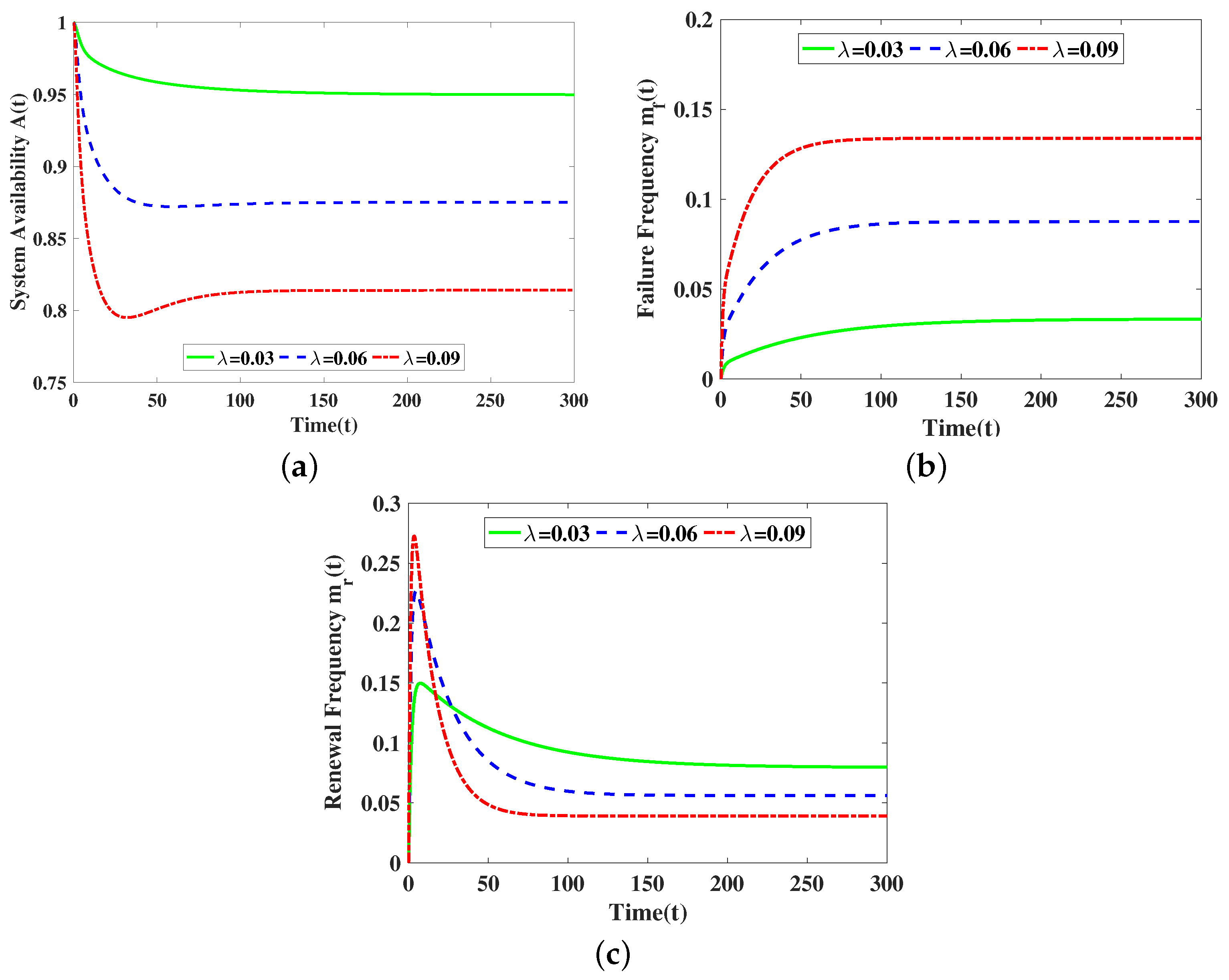
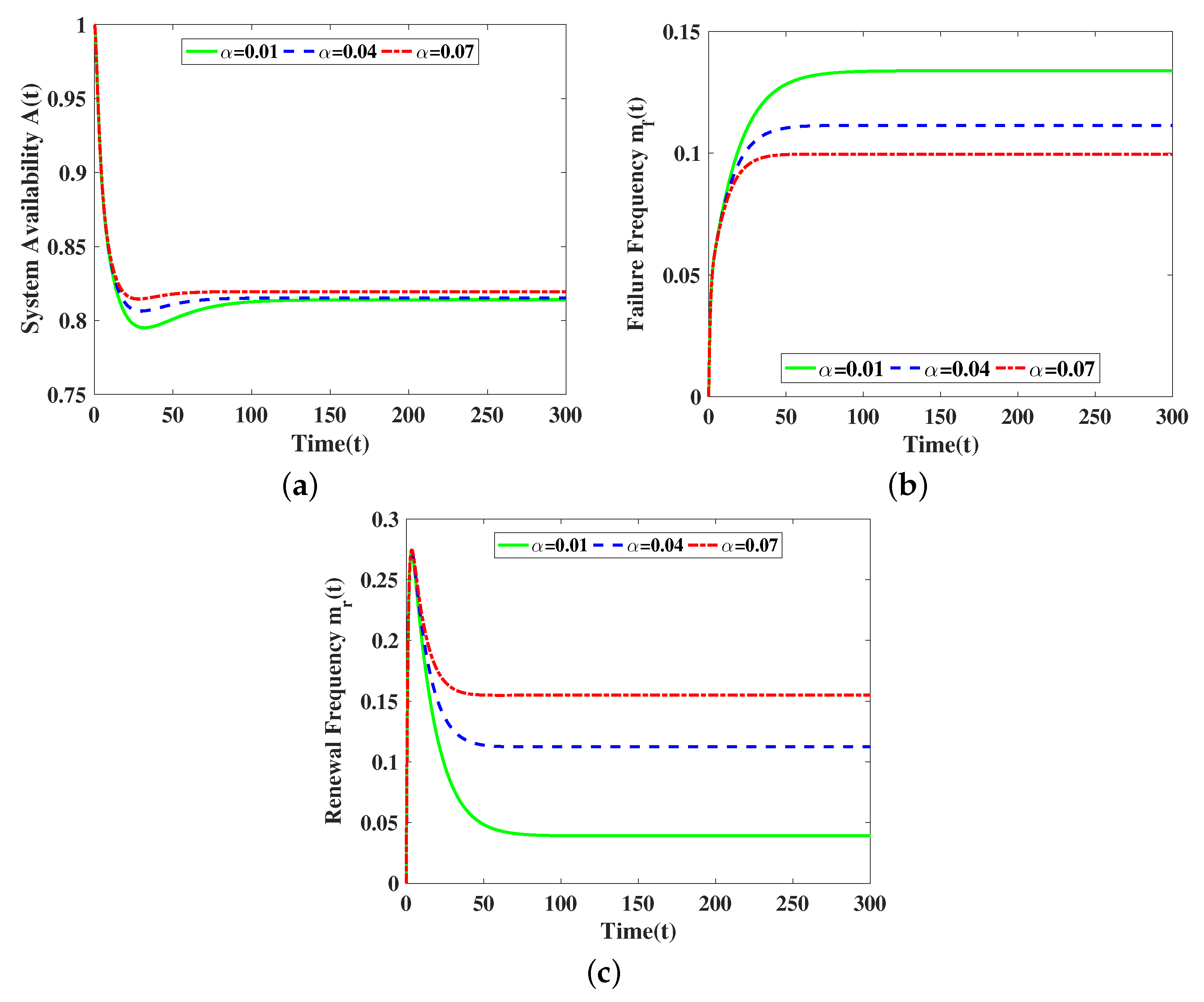
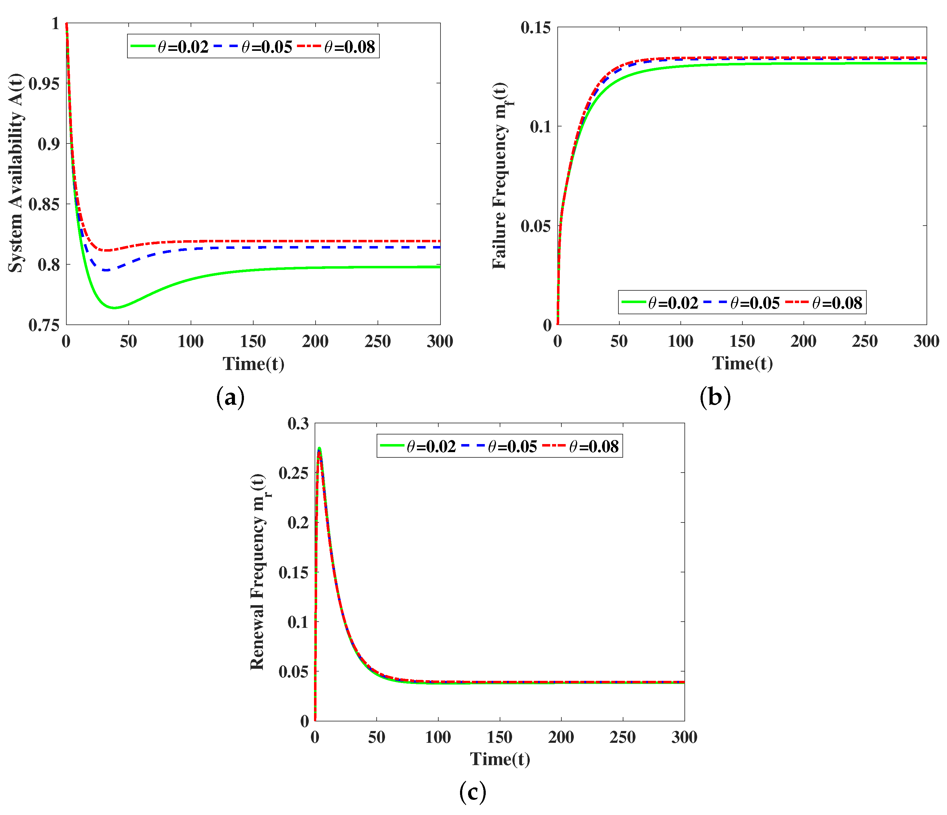
  • The component failure rate, the retry rate for components in orbit, and the repairer’s vacation time are each governed by exponential distributions with the respective parameters λ , θ , and α .
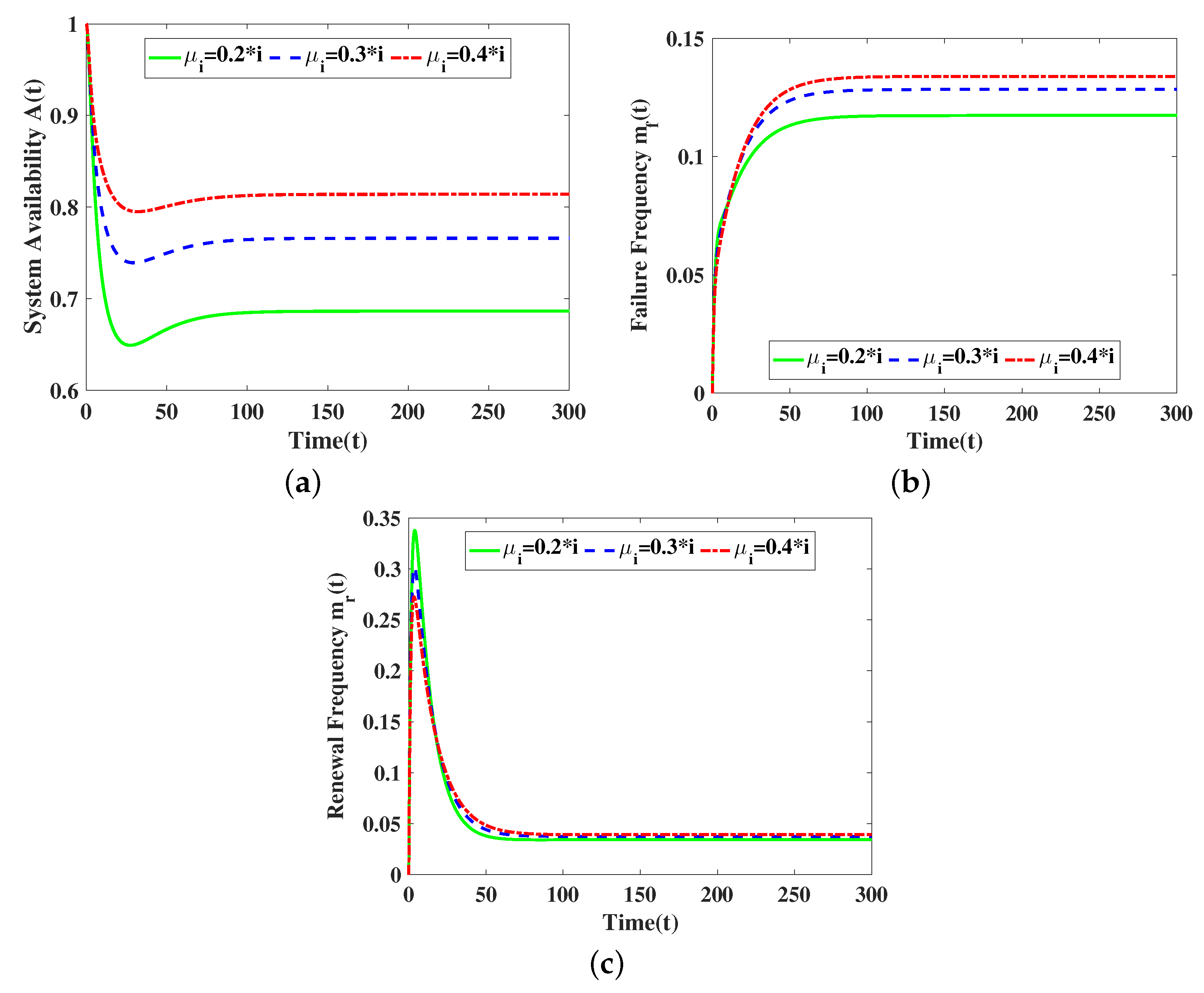
  • The repair rates of the components follow a general distribution. ς 1 ( x ) denotes the repair rate during the repairer’s WV, and ς 2 ( x ) represents the repair rate during a regular busy period. Both satisfy ς l ( x ) 0 , 0 ς l ( x ) d x = , ( l = 1 , 2 ) .
  • The failure probability of each component is independent of the others. All the above five random variables are independent of each other.
Before introducing the system model, we provide the following definitions.
G i , 0 ( t ) ( i = 0 , 1 ) is the probability that there is no failed component on the orbit and the repairer is in a WV period at time t.
G i , 1 ( t , x ) d x ( i = 0 , 1 ) represents the probability that at time t the repairer is in a WV period, with i failed components on the orbit, and the consumed repair time falls in the interval [ x , x + d x ) .
G 1 , 2 ( t ) ( i = 0 , 1 ) is the probability that at time t, there is one failed component on the orbit, and the repairer is idle during a regular busy period.
G i , 3 ( t , x ) d x ( i = 0 , 1 ) represents the probability that at time t the repairer is in a regular busy period, there are i failed components on the orbit, and the elapsed repair time for the failed component is in [ x , x + d x ) .
Taking into account the assumptions of the system outlined above, and using the SVM, we derive the following system of equations:
d G 0 , 0 ( t ) d t = 3 λ G 0 , 0 ( t ) + 0 G 0 , 1 ( t , x ) ς 1 ( x ) d x + 0 G 0 , 3 ( t , x ) ς 2 ( x ) d x ,
d G 1 , 0 ( t ) d t = ( 2 λ + α + θ ) G 1 , 0 ( t ) + 0 G 1 , 1 ( t , x ) ς 1 ( x ) d x ,
G 0 , 1 ( t , x ) t + G 0 , 1 ( t , x ) x = [ 2 λ + θ + ς 1 ( x ) ] G 0 , 1 ( t , x ) ,
G 1 , 1 ( t , x ) t + G 1 , 1 ( t , x ) x = [ θ + ς 1 ( x ) ] G 1 , 1 ( t , x ) + 2 λ G 0 , 1 ( t , x ) ,
d G 1 , 2 ( t ) d t = ( 2 λ + α ) G 1 , 2 ( t ) + 0 G 1 , 3 ( t , x ) ς 2 ( x ) d x + θ G 1 , 0 ( t ) ,
G 0 , 3 ( t , x ) t + G 0 , 3 ( t , x ) x = [ 2 λ + ς 2 ( x ) ] G 0 , 3 ( t , x ) ,
G 1 , 3 ( t , x ) t + G 1 , 3 ( t , x ) x = ς 2 ( x ) G 1 , 3 ( t , x ) + 2 λ G 0 , 3 ( t , x ) .
with the boundary and initial conditions being as follows:
G 0 , 1 ( t , 0 ) = 3 λ G 0 , 0 ( t ) + α G 1 , 0 ( t ) ,
G 1 , 1 ( t , 0 ) = 2 λ G 1 , 0 ( t ) ,
G 0 , 3 ( t , 0 ) = α G 1 , 2 ( t ) + θ 0 G 0 , 1 ( t , x ) d x ,
G 1 , 3 ( t , 0 ) = 2 λ G 1 , 2 ( t ) + θ 0 G 1 , 1 ( t , x ) d x ,
G 0 , 0 ( 0 ) = 1 , G 1 , 0 ( 0 ) = G 1 , 2 ( 0 ) = G i , j ( 0 , x ) = 0 , ( i = 0 , 1 j = 1 , 3 ) .
where ( t , x ) [ 0 , ) × [ 0 , ) .

2.2. Reset the Model

Let us consider the state space to be as for:
X = G G = ( G 0 , 0 , G 1 , 0 , G 0 , 1 , G 1 , 1 , G 1 , 2 , G 0 , 3 , G 1 , 3 ) , G 0 , 0 , G 1 , 0 , G 1 , 2 R , G 0 , 1 ( x ) , G 1 , 1 ( x ) , G 0 , 3 ( x ) , G 1 , 3 ( x ) L 1 [ 0 , ) , G = i = 0 1 | G i , 0 | + i = 0 1 G i , 1 L 1 [ 0 , ) + | G 1 , 2 | + i = 0 1 G i , 3 L 1 [ 0 , ) .
X is a Banach space.
The maximal operator ( S m , D ( S m ) ) (see Greiner [41]) is defined as follows:
S m G = 3 λ 0 ψ 1 0 0 ψ 2 0 0 ( 2 λ + α + θ ) 0 ψ 1 0 0 0 0 0 ϕ 0 1 0 0 0 0 0 0 2 λ ϕ 1 0 0 0 0 θ 0 0 ( 2 λ + α ) 0 ψ 2 0 0 0 0 0 ϕ 0 2 0 0 0 0 0 0 2 λ ϕ 2 G ,
D ( S m ) = G X d G i , j d x L 1 [ 0 , ) , G i , j ( x ) are absolutely continuous functions and i = 0 1 d G i , 1 d x L 1 [ 0 , ) + i = 0 1 d G i , 3 d x L 1 [ 0 , ) < .
Then, let us consider
ψ 1 ϱ : = 0 ς 1 ( x ) ϱ ( x ) d x , ψ 1 : L 1 [ 0 , ) R , ϱ L 1 ( 0 , ) , ψ 2 ϱ : = 0 ς 2 ( x ) ϱ ( x ) d x , ψ 2 : L 1 [ 0 , ) R , ϱ L 1 ( 0 , ) , ϕ 0 1 ϱ : = d ϱ ( x ) d x [ 2 λ + θ + ς 1 ( x ) ] ϱ ( x ) , ϱ W 1 , 1 [ 0 , ) , ϕ 1 ϱ : = d ϱ ( x ) d x [ θ + ς 1 ( x ) ] ϱ ( x ) , ϱ W 1 , 1 [ 0 , ) , ϕ 0 2 ϱ : = d ϱ ( x ) d x [ 2 λ + ς 2 ( x ) ] ϱ ( x ) , ϱ W 1 , 1 [ 0 , ) , ϕ 2 ϱ : = d ϱ ( x ) d x ς 2 ( x ) ϱ ( x ) , ϱ W 1 , 1 [ 0 , ) .
Following boundary space and operators:
X = R 4 , Θ : D ( S m ) X ,
Θ G = G 0 , 1 ( 0 ) G 1 , 1 ( 0 ) G 0 , 3 ( 0 ) G 1 , 3 ( 0 ) ,
and
Ψ : D ( S m ) X ,
Ψ G = 3 λ α 0 0 0 0 0 0 2 λ 0 0 0 0 0 0 0 θ φ 0 α 0 0 0 0 0 θ φ 2 λ 0 0 G ,
where
φ ϱ : = 0 ϱ ( x ) d x , ϱ L 1 ( 0 , ) .
If we define operator S ¯ as
S ¯ G = S m G , D ( S ¯ ) = G D ( S m ) | Θ G = Ψ G .
The aforementioned Equations (1)–(12) can be rewritten as an ACP in the X.
d G ( t ) d t = S m G ( t ) , t ( 0 , ) , G ( 0 ) = ( 1 , 0 , 0 , 0 , 0 , 0 , 0 ) .

3. Well−Posedness of System

Firstly, we demonstrate that the operator S ¯ generates a positive contraction C 0 semigroup T ( t ) . Next we show that S ¯ is a conservative operator and furthermore obtain that T ( t ) is isometric. This establishes the well−posedness of the system.
Theorem 1. 
Let ς l = sup x [ 0 , ) ς l ( x ) < ( l = 1 , 2 ) ; then, S ¯ generates a positive contraction C 0 semigroup T ( t ) .
The proof can be found in Appendix A.
The dual space X * of X is defined as follows:
X * = G * G * = ( G 0 , 0 * , G 1 , 0 * , G 0 , 1 * , G 1 , 1 * , G 1 , 2 * , G 0 , 3 * , G 1 , 3 * ) , G 0 , 0 * , G 1 , 0 * , G 1 , 2 * R , G 0 , 1 * ( x ) , G 1 , 1 * ( x ) , G 0 , 3 * ( x ) , G 1 , 3 * ( x ) L [ 0 , ) , | | | G * | | | = max { | G 0 , 0 * | , | G 1 , 0 * | , | G 1 , 2 * | , G 0 , 1 * L [ 0 , ) , G 1 , 1 * L [ 0 , ) , G 0 , 3 * L [ 0 , ) , G 1 , 3 * L [ 0 , ) } .
X * is a Banach space. In space X, we define the subset
Y = G X G = ( G 0 , 0 , G 1 , 0 , G 0 , 1 ( x ) , G 1 , 1 ( x ) , G 1 , 2 , G 0 , 3 ( x ) , G 1 , 3 ( x ) ) , G i , 0 0 , G 1 , 2 0 , G i , j ( x ) 0 , i = 0 , 1 , j = 1 , 3 , x [ 0 , ) .
According to Theorem 1, we can conclude that T ( t ) Y Y . For G D ( S ¯ ) Y , we take G * = G ( 1 , 1 , 1 , 1 , 1 , 1 , 1 ) ; then, G * X * and
S ¯ G , G * = 3 λ G 0 , 0 + 0 G 0 , 1 ( x ) ς 1 ( x ) d x + 0 G 0 , 3 ( x ) ς 2 ( x ) d x G + ( 2 λ + α + θ ) G 1 , 0 + 0 G 1 , 1 ( x ) ς 1 ( x ) d x G + 0 d G 0 , 1 ( x ) d x [ 2 λ + θ + ς 1 ( x ) ] G 0 , 1 ( x ) G d x + 0 d G 1 , 1 ( x ) d x [ θ + ς 1 ( x ) ] G 1 , 1 ( x ) + 2 λ G 0 , 1 ( x ) G d x + ( 2 λ + α ) G 1 , 2 + 0 G 1 , 3 ( x ) ς 2 ( x ) d x + θ G 1 , 0 G + 0 d G 0 , 3 ( x ) d x [ 2 λ + ς 2 ( x ) ] G 0 , 3 ( x ) G d x + 0 d G 1 , 3 ( x ) d x ς 2 ( x ) G 1 , 3 ( x ) + 2 λ G 0 , 3 ( x ) G d x = G 3 λ G 0 , 0 + G 0 G 0 , 1 ( x ) ς 1 ( x ) d x + G 0 G 0 , 3 ( x ) ς 2 ( x ) d x G ( 2 λ + α + θ ) G 1 , 0 + G 0 G 1 , 1 ( x ) ς 1 ( x ) d x + G G 0 , 1 ( 0 ) G 0 G 0 , 1 ( x ) [ 2 λ + θ + ς 1 ( x ) ] d x + G G 1 , 1 ( 0 ) G 0 G 1 , 1 ( x ) [ θ + ς 1 ( x ) ] d x + G 0 2 λ G 0 , 1 ( x ) d x G ( 2 λ + α ) G 1 , 2 + G θ G 1 , 0 + G 0 G 1 , 3 ( x ) ς 2 ( x ) d x + G G 0 , 3 ( 0 ) G 0 G 0 , 3 ( x ) [ 2 λ + ς 2 ( x ) ] d x + G G 1 , 3 ( 0 ) G 0 G 1 , 3 ( x ) ς 2 ( x ) d x + G 0 2 λ G 0 , 3 ( x ) d x = 0 .
Thus, S ¯ is conservative for the set
ϖ ( G ) = { G * X * | G , G * = G 2 = | | | G * | | | 2 } .
Since G ( 0 ) D ( S ¯ 2 ) Y , the following result was obtained by applying Fattorini’s method [42].
Theorem 2. 
T ( t ) is isometric for G ( 0 ) , i.e.,
T ( t ) G ( 0 ) = G ( 0 ) , t [ 0 , ) .
By combining Theorem 1 with Theorem 2 we obtain the desired result in this section.
Theorem 3. 
Let ς l = sup x [ 0 , ) ς l ( x ) < ( l = 1 , 2 ) ; then system (13) has a unique nonnegative TDS G ( t , x ) that satisfies
G ( t , · ) = 1 , t [ 0 , ) .
Proof. 
Since G ( 0 ) D ( S ¯ 2 ) Y , by Theorems 1 and 1.81 [40], we obtain that system (13) has a unique positive TDS G ( t , x ) which can be expressed as
G ( t , x ) = T ( t ) G ( 0 ) , t [ 0 , ) .
By Theorem 2, it has
G ( t , · ) = T ( t ) G ( 0 ) = G ( 0 ) = 1 , t [ 0 , ) .
This justifies the physics reflected by G ( t , x ) . □

4. Asymptotic Behavior of the TDS of System

By looking at the system (13), we realize that the key to the solution lies in the boundary conditions. In 1987, Greiner [41] introduced the idea of studying the spectrum of S ¯ by perturbing the boundary conditions. In this section, we use this method to obtain the spectrum of S ¯ on the imaginary axis, thus obtaining the asymptotic behavior of the TDS of system (13).
Lemma 1. 
Let
2 λ + α + θ > 0 [ 2 λ + α ( 1 e 2 λ x ) ] e θ x 0 x ς 1 ( ϑ ) d ϑ ς 1 ( x ) d x ,
0 e 2 λ x 0 x ς 2 ( ϑ ) d ϑ ς 2 ( x ) d x < ,
then, 0 σ p ( S ¯ ) and the geometric multiplicity is 1.
Proof. 
For the Equation S ¯ G = 0 , i.e.,
3 λ G 0 , 0 = 0 G 0 , 1 ( x ) ς 1 ( x ) d x + 0 G 0 , 3 ( x ) ς 2 ( x ) d x ,
( 2 λ + α + θ ) G 1 , 0 = 0 G 1 , 1 ( x ) ς 1 ( x ) d x ,
d G 0 , 1 ( x ) d x = 2 λ + θ + ς 1 ( x ) G 0 , 1 ( x ) ,
d G 1 , 1 ( x ) d x = θ + ς 1 ( x ) G 1 , 1 ( x ) + 2 λ G 0 , 1 ( x ) ,
( 2 λ + α ) G 1 , 2 = 0 G 1 , 3 ( x ) ς 2 ( x ) d x + θ G 1 , 0 ,
d G 0 , 3 ( x ) d x = 2 λ + ς 2 ( x ) G 0 , 3 ( x ) ,
d G 1 , 3 ( x ) d x = ς 2 ( x ) G 1 , 3 ( x ) + 2 λ G 0 , 3 ( x ) ,
G 0 , 1 ( 0 ) = 3 λ G 0 , 0 + α G 1 , 0 ,
G 1 , 1 ( 0 ) = 2 λ G 1 , 0 ,
G 0 , 3 ( 0 ) = α G 1 , 2 + θ 0 G 0 , 1 ( x ) d x ,
G 1 , 3 ( 0 ) = 2 λ G 1 , 2 + θ 0 G 1 , 1 ( x ) d x .
By solving Equations (16), (17), (19) and (20) and using Equations (21)–(24) we obtain
G 0 , 1 ( x ) = e 2 λ x θ x 0 x ς 1 ( ϑ ) d ϑ ( 3 λ G 0 , 0 + α G 1 , 0 ) ,
G 1 , 1 ( x ) = e θ x 0 x ς 1 ( ϑ ) d ϑ 2 λ G 1 , 0 + ( 1 e 2 λ x ) ( 3 λ G 0 , 0 + α G 1 , 0 ) ,
G 0 , 3 ( x ) = e 2 λ x 0 x ς 2 ( ϑ ) d ϑ α G 1 , 2 + θ 0 G 0 , 1 ( x ) d x ,
G 1 , 3 ( x ) = e 0 x ς 2 ( ϑ ) d ϑ [ 2 λ G 1 , 2 + θ 0 G 1 , 1 ( x ) d x + ( 1 e 2 λ x ) α G 1 , 2 + θ 0 G 0 , 1 ( x ) d x ] .
Substituting Equations (25) and (26) into Equations (27) and (28) gives
G 0 , 3 ( x ) = e 2 λ x 0 x ς 2 ( ϑ ) d ϑ × α G 1 , 2 + θ ( 3 λ G 0 , 0 + α G 1 , 0 ) 0 e 2 λ x θ x 0 x ς 1 ( ϑ ) d ϑ d x ,
G 1 , 3 ( x ) = e 0 x ς 2 ( ϑ ) d ϑ [ 2 λ G 1 , 2 + α G 1 , 2 ( 1 e 2 λ x ) + 2 λ θ G 1 , 0 0 e θ x 0 x ς 1 ( ϑ ) d ϑ d x + θ ( 3 λ G 0 , 0 + α G 1 , 0 ) 0 e θ x 0 x ς 1 ( ϑ ) d ϑ d x θ 3 λ G 0 , 0 + α G 1 , 0 e 2 λ x 0 e 2 λ x θ x 0 x ς 1 ( ϑ ) d ϑ d x ] .
Combining Equations (26) and (30) with Equations (15) and (18) we have
G 1 , 0 = 3 λ 0 ( 1 e 2 λ x ) e θ x 0 x ς 1 ( ϑ ) d ϑ ς 1 ( x ) d x 2 λ + α + θ 0 [ 2 λ + α ( 1 e 2 λ x ) ] e θ x 0 x ς 1 ( ϑ ) d ϑ ς 1 ( x ) d x G 0 , 0 ,
G 1 , 2 = Π α 0 e 2 λ x 0 x ς 2 ( ϑ ) d ϑ ς 2 ( x ) d x G 0 , 0 .
where
Π = 3 λ θ { [ 0 e θ x 0 x ς 1 ( ϑ ) d ϑ d x 0 e 2 λ x θ x 0 x ς 1 ( ϑ ) d ϑ d x 0 e 2 λ x 0 x ς 2 ( ϑ ) d ϑ ς 2 ( x ) d x ] + [ 1 + ( 2 λ + α ) 0 e θ x 0 x ς 1 ( ϑ ) d ϑ d x α 0 e 2 λ x θ x 0 x ς 1 ( ϑ ) d ϑ d x 0 e 2 λ x 0 x ς 2 ( ϑ ) d ϑ ς 2 ( x ) d x ] × 0 ( 1 e 2 λ x ) e θ x 0 x ς 1 ( ϑ ) d ϑ ς 1 ( x ) d x 2 λ + α + θ 0 [ 2 λ + α ( 1 e 2 λ x ) ] e θ x 0 x ς 1 ( ϑ ) d ϑ ς 1 ( x ) d x } .
From Equations (25), (26), and (29)–(32) we estimate
G G 0 , 0 + G 1 , 0 + G 1 , 2 + 3 λ G 0 , 0 + α G 1 , 0 0 e 2 λ x θ x 0 x ς 1 ( ϑ ) d ϑ d x + 3 λ G 0 , 0 + ( 2 λ + α ) G 1 , 0 0 e θ x 0 x ς 1 ( ϑ ) d ϑ d x + 3 λ G 0 , 0 + α G 1 , 0 0 e 2 λ x θ x 0 x ς 1 ( ϑ ) d ϑ d x + α G 1 , 2 + θ 3 λ G 0 , 0 + α G 1 , 0 0 e 2 λ x θ x 0 x ς 1 ( ϑ ) d ϑ d x × 0 e 2 λ x 0 x ς 2 ( ϑ ) d ϑ d x + ( 2 λ + α ) G 1 , 2 0 e 0 x ς 2 ( ϑ ) d ϑ d x + θ 3 λ G 0 , 0 + ( 2 λ + α ) G 1 , 0 0 e θ x 0 x ς 1 ( ϑ ) d ϑ d x 0 e 0 x ς 2 ( ϑ ) d ϑ d x + α G 1 , 2 + θ 3 λ G 0 , 0 + α G 1 , 0 0 e 2 λ x θ x 0 x ς 1 ( ϑ ) d ϑ d x × 0 e 2 λ x 0 x ς 2 ( ϑ ) d ϑ d x { [ 1 + 6 λ 0 e 2 λ x θ x 0 x ς 1 ( ϑ ) d ϑ d x + 3 λ 0 e θ x 0 x ς 1 ( ϑ ) d ϑ d x + 6 λ θ 0 e 2 λ x θ x 0 x ς 1 ( ϑ ) d ϑ d x 0 e 2 λ x 0 x ς 2 ( ϑ ) d ϑ d x + 3 λ θ 0 e θ x 0 x ς 1 ( ϑ ) d ϑ d x 0 e 0 x ς 2 ( ϑ ) d ϑ d x ] + [ 1 + 2 α 0 e 2 λ x θ x 0 x ς 1 ( ϑ ) d ϑ d x + ( 2 λ + α ) 0 e θ x 0 x ς 1 ( ϑ ) d ϑ d x + 2 α θ 0 e 2 λ x θ x 0 x ς 1 ( ϑ ) d ϑ d x 0 e 2 λ x 0 x ς 2 ( ϑ ) d ϑ d x + θ ( 2 λ + α ) 0 e θ x 0 x ς 1 ( ϑ ) d ϑ d x 0 e 0 x ς 2 ( ϑ ) d ϑ d x ] × 3 λ 0 1 e 2 λ x e θ x 0 x ς 1 ( ϑ ) d ϑ ς 1 ( x ) d x 2 λ + α + θ 0 2 λ + α 1 e 2 λ x e θ x 0 x ς 1 ( ϑ ) d ϑ ς 1 ( x ) d x + 1 + 2 α 0 e 2 λ x 0 x ς 2 ( ϑ ) d ϑ d x + ( 2 λ + α ) 0 e 0 x ς 2 ( ϑ ) d ϑ d x × Π α 0 e 2 λ x 0 x ς 2 ( ϑ ) d ϑ ς 2 ( x ) d x } G 0 , 0 < .
This demonstrates that 0 is an eigenvalue of S ¯ . Furthermore, Equations (25), (26), and (29)–(32) mean that the GM of 0 is 1. □
Subsequently, we apply Greiner’s ideas [41] to investigate the resolvent set of S ¯ on the imaginary axis. If we define ( S 0 , D ( S 0 ) ) as
S 0 G = S m G , D ( S 0 ) = G D ( S m ) | Θ G = 0 ,
then for any given W = ( W 0 , 0 , W 1 , 0 , W 0 , 1 , W 1 , 1 , W 1 , 2 , W 0 , 3 , W 1 , 3 ) X , for the Equation ( γ I S 0 ) G = W , i.e.,
( γ + 3 λ ) G 0 , 0 = 0 G 0 , 1 ( x ) ς 1 ( x ) d x + 0 G 0 , 3 ( x ) ς 2 ( x ) d x + W 0 , 0 ,
( γ + 2 λ + α + θ ) G 1 , 0 = 0 G 1 , 1 ( x ) ς 1 ( x ) d x + W 1 , 0 ,
d G 0 , 1 ( x ) d x = γ + 2 λ + θ + ς 1 ( x ) G 0 , 1 ( x ) + W 0 , 1 ( x ) ,
d G 1 , 1 ( x ) d x = γ + θ + ς 1 ( x ) G 1 , 1 ( x ) + 2 λ G 0 , 1 ( x ) + W 1 , 1 ( x ) ,
( γ + 2 λ + α ) G 1 , 2 = 0 G 1 , 3 ( x ) ς 2 ( x ) d x + θ G 1 , 0 + W 1 , 2 ,
d G 0 , 3 ( x ) d x = γ + 2 λ + ς 2 ( x ) G 0 , 3 ( x ) + W 0 , 3 ( x ) ,
d G 1 , 3 ( x ) d x = γ + ς 2 ( x ) G 1 , 3 ( x ) + 2 λ G 0 , 3 ( x ) + W 1 , 3 ( x ) ,
G i , j ( 0 ) = 0 , i = 0 , 1 , j = 1 , 3 .
Solving Equations (33)–(39) and combining them with Equation (40), we obtain
G 0 , 0 = 1 γ + 3 λ W 0 , 0 + 1 γ + 3 λ 0 G 0 , 1 ( x ) ς 1 ( x ) d x + 1 γ + 3 λ 0 G 0 , 3 ( x ) ς 2 ( x ) d x ,
G 1 , 0 = 1 γ + 2 λ + α + θ W 1 , 0 + 1 γ + 2 λ + α + θ 0 G 1 , 1 ( x ) ς 1 ( x ) d x ,
G 0 , 1 ( x ) = e 0 x [ γ + 2 λ + θ + ς 1 ( ϑ ) ] d ϑ 0 x W 0 , 1 ( ϑ ) e 0 ϑ [ γ + 2 λ + θ + ς 1 ( ω ) ] d ω d ϑ ,
G 1 , 1 ( x ) = e 0 x [ γ + θ + ς 1 ( ϑ ) ] d ϑ 0 x W 1 , 1 ( ϑ ) e 0 ϑ [ γ + θ + ς 1 ( ω ) ] d ω d ϑ
+ e 0 x [ γ + θ + ς 1 ( ϑ ) ] d ϑ 0 x 2 λ G 0 , 1 ( ϑ ) e 0 ϑ [ γ + θ + ς 1 ( ω ) ] d ω d ϑ ,
G 1 , 2 = 1 γ + 2 λ + α W 1 , 2 + θ γ + 2 λ + α G 1 , 0 + 1 γ + 2 λ + α 0 G 1 , 3 ( x ) ς 2 ( x ) d x ,
G 0 , 3 ( x ) = e 0 x [ γ + 2 λ + ς 2 ( ϑ ) ] d ϑ 0 x W 0 , 3 ( ϑ ) e 0 ϑ [ γ + 2 λ + ς 2 ( ω ) ] d ω d ϑ ,
G 1 , 3 ( x ) = e 0 x [ γ + ς 2 ( ϑ ) ] d ϑ 0 x W 1 , 3 ( ϑ ) e 0 ϑ [ γ + ς 2 ( ω ) ] d ω d ϑ + e 0 x [ γ + ς 2 ( ϑ ) ] d ϑ 0 x 2 λ G 0 , 3 ( ϑ ) e 0 ϑ [ γ + ς 2 ( ω ) ] d ω d ϑ .
For any ϱ L 1 [ 0 , ) , if we set
E 1 ϱ ( x ) = e 0 x [ γ + 2 λ + θ + ς 1 ( ϑ ) ] d ϑ 0 x ϱ ( ϑ ) e 0 ϑ [ γ + 2 λ + θ + ς 1 ( ω ) ] d ω d ϑ ,
E ˜ 1 ϱ ( x ) = e 0 x [ γ + θ + ς 1 ( ϑ ) ] d ϑ 0 x ϱ ( ϑ ) e 0 ϑ [ γ + θ + ς 1 ( ω ) ] d ω d ϑ ,
E 2 ϱ ( x ) = e 0 x [ γ + 2 λ + ς 2 ( ϑ ) ] d ϑ 0 x ϱ ( ϑ ) e 0 ϑ [ γ + 2 λ + ς 2 ( ω ) ] d ω d ϑ ,
E ˜ 2 ϱ ( x ) = e 0 x [ γ + ς 2 ( ϑ ) ] d ϑ 0 x ϱ ( ϑ ) e 0 ϑ [ γ + ς 2 ( ω ) ] d ω d ϑ .
By applying ψ l ϱ ( x ) = 0 ϱ ( x ) ς l ( x ) d x ( l = 1 , 2 ) , Equations (41)–(47) can be simplified as follows:
G 0 , 0 = 1 γ + 3 λ W 0 , 0 + 1 γ + 3 λ ψ 1 E 1 W 0 , 1 ( x ) + 1 γ + 3 λ ψ 2 E 2 W 0 , 3 ( x ) ,
G 1 , 0 = 1 γ + 2 λ + α + θ W 1 , 0 + 1 γ + 2 λ + α + θ ψ 1 E ˜ 1 W 1 , 1 ( x ) + 2 λ γ + 2 λ + α + θ ψ 1 E ˜ 1 E 1 W 0 , 1 ( x ) ,
G 0 , 1 ( x ) = E 1 W 0 , 1 ( x ) ,
G 1 , 1 ( x ) = E ˜ 1 W 1 , 1 ( x ) + 2 λ E ˜ 1 E 1 W 0 , 1 ( x ) ,
G 1 , 2 = 1 γ + 2 λ + α W 1 , 2 + θ ( γ + 2 λ + α ) ( γ + 2 λ + α + θ ) × W 1 , 0 + ψ 1 E ˜ 1 W 1 , 1 ( x ) + 2 λ ψ 1 E ˜ 1 E 1 W 0 , 1 ( x ) + 1 γ + 2 λ + α ψ 2 E ˜ 2 W 1 , 3 ( x ) + 2 λ γ + 2 λ + α ψ 2 E ˜ 2 E 2 W 0 , 3 ( x ) ,
G 0 , 3 ( x ) = E 2 W 0 , 3 ( x ) ,
G 1 , 3 ( x ) = E ˜ 2 W 1 , 3 ( x ) + 2 λ E ˜ 2 E 2 W 0 , 3 ( x ) .
According to Equations (52)–(58), we get
( γ I S 0 ) 1 W = 1 γ + 3 λ 0 ψ 1 E 1 γ + 3 λ 0 0 ψ 2 E 2 γ + 3 λ 0 0 1 γ + 2 λ + α + θ 2 λ ψ 1 E ˜ 1 E 1 γ + 2 λ + α + θ ψ 1 E ˜ 1 γ + 2 λ + α + θ 0 0 0 0 0 E 1 0 0 0 0 0 0 2 λ E ˜ 1 E 1 E ˜ 1 0 0 0 0 θ Λ 2 λ θ ψ 1 E ˜ 1 E 1 Λ θ ψ 1 E ˜ 1 Λ 1 γ + 2 λ + α 2 λ ψ 2 E ˜ 2 E 2 γ + 2 λ + α ψ 2 E ˜ 2 γ + 2 λ + α 0 0 0 0 0 E 2 0 0 0 0 0 0 2 λ E ˜ 2 E 2 E ˜ 2 W ,
where Λ = ( γ + 2 λ + α ) ( γ + 2 λ + α + θ ) .
According to the definition of the resolvent set, we can obtain the following result.
Lemma 2. 
Let ς l ( x ) : [ 0 , ) [ 0 , ) be measurable and
0 < inf x [ 0 , ) ς l ( x ) < sup x [ 0 , ) ς l ( x ) < , l = 1 , 2 ,
then,
γ C Re γ + inf x [ 0 , ) ς l ( x ) > 0 , l = 1 , 2 ρ ( S 0 ) ,
which shows that all points on the imaginary axis belong to ρ ( S 0 ) .
Proof. 
For any ϱ L 1 [ 0 , ) C 0 [ 0 , ) , we estimate
0 E 1 ϱ ( x ) d x 0 e ( Re γ + 2 λ + θ ) x 0 x ς 1 ( ϑ ) d ϑ 0 x | ϱ ( ϑ ) | e ( Re γ + 2 λ + θ ) ϑ + 0 ϑ ς 1 ( ω ) d ω d ϑ d x = 0 1 Re γ + 2 λ + θ + ς 1 ( x ) 0 x | ϱ ( ϑ ) | e ( Re γ + 2 λ + θ ) ϑ + 0 ϑ ς 1 ( ω ) d ω d ϑ × d e ( Re γ + 2 λ + θ ) x 0 x ς 1 ( ϑ ) d ϑ = 1 Re γ + 2 λ + θ + inf x [ 0 , ) ς 1 ( x ) { e ( Re γ + 2 λ + θ ) x 0 x ς 1 ( ϑ ) d ϑ × 0 x | ϱ ( ϑ ) | e ( Re γ + 2 λ + θ ) ϑ + 0 ϑ ς 1 ( ω ) d ω d ϑ | x = 0 x = 0 e ( Re γ + 2 λ + θ ) x 0 x ς 1 ( ϑ ) d ϑ × e ( Re γ + 2 λ + θ ) x + 0 x ς 1 ( ϑ ) d ϑ | ϱ ( x ) | d x } = 1 Re γ + 2 λ + θ + inf x [ 0 , ) ς 1 ( x ) { lim x e ( Re γ + 2 λ + θ ) x 0 x ς 1 ( ϑ ) d ϑ × 0 x | ϱ ( ϑ ) | e ( Re γ + 2 λ + θ ) ϑ + 0 ϑ ς 1 ( ω ) d ω d ϑ + 0 | ϱ ( x ) | d x } 1 Re γ + 2 λ + θ + inf x [ 0 , ) ς 1 ( x ) ϱ L 1 [ 0 , ) .
Similarly,
0 E ˜ 1 ϱ ( x ) d x 1 Re γ + θ + inf x [ 0 , ) ς 1 ( x ) ϱ L 1 [ 0 , ) .
0 E 2 ϱ ( x ) d x 1 Re γ + 2 λ + inf x [ 0 , ) ς 2 ( x ) ϱ L 1 [ 0 , ) .
0 E ˜ 2 ϱ ( x ) d x 1 Re γ + inf x [ 0 , ) ς 2 ( x ) ϱ L 1 [ 0 , ) .
According to Adams [43], C 0 [ 0 , ) is dense in L 1 [ 0 , ) , and it follows that Equations (60)–(63) hold for all ϱ L 1 [ 0 , ) .
By using Equations (59)–(63) with the condition Re γ + inf x [ 0 , ) ς l ( x ) > 0 ( l = 1 , 2 ) we estimate, for W X ,
( γ I A 0 ) 1 W 1 γ + 3 λ W 0 , 0 + 1 γ + 3 λ ψ 1 E 1 W 0 , 1 + 1 γ + 3 λ ψ 2 E 2 W 0 , 3 + 1 γ + 2 λ + α + θ W 1 , 0 + 2 λ γ + 2 λ + α + θ ψ 1 E ˜ 1 E 1 W 0 , 1 + 1 γ + 2 λ + α + θ ψ 1 E ˜ 1 W 1 , 1 + E 1 W 0 , 1 + 2 λ E ˜ 1 E 1 W 0 , 1 + E ˜ 1 W 1 , 1 + | θ ( γ + 2 λ + α ) ( γ + 2 λ + α + θ ) W 1 , 0 + 2 λ θ ( γ + 2 λ + α ) ( γ + 2 λ + α + θ ) ψ 1 E ˜ 1 E 1 W 0 , 1 + θ ( γ + 2 λ + α ) ( γ + 2 λ + α + θ ) ψ 1 E ˜ 1 W 1 , 1 + 1 γ + 2 λ + α W 1 , 2 + 2 λ γ + 2 λ + α ψ 2 E ˜ 2 E 2 W 0 , 3 + 1 γ + 2 λ + α ψ 2 E ˜ 2 W 1 , 3 | + E 2 W 0 , 3 + 2 λ E ˜ 2 E 2 W 0 , 3 + E ˜ 2 W 1 , 3 1 | γ + 3 λ | W 0 , 0 + 1 | γ + 2 λ + α + θ | + θ | ( γ + 2 λ + α ) ( γ + 2 λ + α + θ ) | W 1 , 0 + 1 | γ + 2 λ + α | W 1 , 2 + 1 | γ + 3 λ | ψ 1 E 1 + 2 λ | γ + 2 λ + α + θ | ψ 1 E ˜ 1 E 1 + E 1 + 2 λ E ˜ 1 E 1 + 2 λ θ | ( γ + 2 λ + α ) ( γ + 2 λ + α + θ ) | ψ 1 E ˜ 1 E 1 W 0 , 1 L 1 [ 0 , ) + 1 | γ + 2 λ + α + θ | ψ 1 E ˜ 1 + E ˜ 1 + θ | ( γ + 2 λ + α ) ( γ + 2 λ + α + θ ) | ψ 1 E ˜ 1 × W 1 , 1 L 1 [ 0 , ) + 1 | γ + 3 λ | ψ 2 E 2 + 2 λ | γ + 2 λ + α | ψ 2 E ˜ 2 E 2 + E 2 + 2 λ E ˜ 2 E 2 × W 0 , 3 L 1 [ 0 , ) + 1 | γ + 2 λ + α | ψ 2 E ˜ 2 + E ˜ 2 W 1 , 3 L 1 [ 0 , ) sup { 1 Re γ + 2 λ + θ + inf x [ 0 , ) ς 1 ( x ) + 1 | γ + 3 λ | sup x [ 0 , ) ς 1 ( x ) Re γ + 2 λ + θ + inf x [ 0 , ) ς 1 ( x ) + 1 Re γ + θ + inf x [ 0 , ) ς 1 ( x ) 2 λ Re γ + 2 λ + θ + inf x [ 0 , ) ς 1 ( x ) + 2 λ | γ + 2 λ + α + θ | 1 Re γ + θ + inf x [ 0 , ) ς 1 ( x ) sup x [ 0 , ) ς 1 ( x ) Re γ + 2 λ + θ + inf x [ 0 , ) ς 1 ( x ) + 2 λ | ( γ + 2 λ + α ) ( γ + 2 λ + α + θ ) | θ Re γ + θ + inf x [ 0 , ) ς 1 ( x ) sup x [ 0 , ) ς 1 ( x ) Re γ + 2 λ + θ + inf x [ 0 , ) ς 1 ( x ) , 1 Re γ + 2 λ + inf x [ 0 , ) ς 2 ( x ) + 1 | γ + 3 λ | sup x [ 0 , ) ς 2 ( x ) Re γ + 2 λ + inf x [ 0 , ) ς 2 ( x ) + 1 Re γ + inf x [ 0 , ) ς 2 ( x ) 2 λ Re γ + 2 λ + inf x [ 0 , ) ς 2 ( x ) + 2 λ | γ + 2 λ + α | 1 Re γ + inf x [ 0 , ) ς 2 ( x ) sup x [ 0 , ) ς 2 ( x ) Re γ + 2 λ + inf x [ 0 , ) ς 2 ( x ) } W < .
Which completes the proof. □
Lemma 3. 
Let ς l ( x ) : [ 0 , ) [ 0 , ) be measurable and
0 < inf x [ 0 , ) ς l ( x ) < sup x [ 0 , ) ς l ( x ) < , l = 1 , 2 ,
if
γ γ C | Re γ + inf x [ 0 , ) ς l ( x ) > 0 , l = 1 , 2 ,
then,
G ker ( γ I S m ) G = G 0 , 0 , G 1 , 0 , G 0 , 1 ( x ) , G 1 , 1 ( x ) , G 1 , 2 , G 0 , 3 ( x ) , G 1 , 3 ( x ) G 0 , 0 = 1 γ + 3 λ [ 0 a 0 , 1 e ( γ + 2 λ + θ ) x 0 x ς 1 ( ϑ ) d ϑ ς 1 ( x ) d x + 0 a 0 , 3 e ( γ + 2 λ ) x 0 x ς 2 ( ϑ ) d ϑ ς 2 ( x ) d x ] ,
G 1 , 0 = 1 γ + 2 λ + α + θ [ 0 a 1 , 1 e ( γ + θ ) x 0 x ς 1 ( ϑ ) d ϑ ς 1 ( x ) d x + 0 a 0 , 1 1 e 2 λ x e ( γ + θ ) x 0 x ς 1 ( ϑ ) d ϑ ς 1 ( x ) d x ] ,
G 0 , 1 ( x ) = a 0 , 1 e ( γ + 2 λ + θ ) x 0 x ς 1 ( ϑ ) d ϑ ,
G 1 , 1 ( x ) = a 1 , 1 + a 0 , 1 1 e 2 λ x e ( γ + θ ) x 0 x ς 1 ( ϑ ) d ϑ ,
G 1 , 2 = 1 γ + 2 λ + α { 0 a 1 , 3 + a 0 , 3 1 e 2 λ x e γ x 0 x ς 2 ( ϑ ) d ϑ ς 2 ( x ) d x + θ γ + 2 λ + α + θ 0 a 1 , 1 + a 0 , 1 1 e 2 λ x e ( γ + θ ) x 0 x ς 1 ( ϑ ) d ϑ ς 1 ( x ) d x } ,
G 0 , 3 ( x ) = a 0 , 3 e ( γ + 2 λ ) x 0 x ς 2 ( ϑ ) d ϑ ,
G 1 , 3 ( x ) = a 1 , 3 + a 0 , 3 1 e 2 λ x e γ x 0 x ς 2 ( ϑ ) d ϑ .
Proof. 
If G ker ( γ I S m ) , then ( γ I S m ) G = 0 , i.e.,
( γ + 3 λ ) G 0 , 0 = 0 G 0 , 1 ( x ) ς 1 ( x ) d x + 0 G 0 , 3 ( x ) ς 2 ( x ) d x ,
( γ + 2 λ + α + θ ) G 1 , 0 = 0 G 1 , 1 ( x ) ς 1 ( x ) d x ,
d G 0 , 1 ( x ) d x = γ + 2 λ + θ + ς 1 ( x ) G 0 , 1 ( x ) ,
d G 1 , 1 ( x ) d x = γ + θ + ς 1 ( x ) G 1 , 1 ( x ) + 2 λ G 0 , 1 ( x ) ,
( γ + 2 λ + α ) G 1 , 2 = 0 G 1 , 3 ( x ) ς 2 ( x ) d x + θ G 1 , 0 ,
d G 0 , 3 ( x ) d x = γ + 2 λ + ς 2 ( x ) G 0 , 3 ( x ) ,
d G 1 , 3 ( x ) d x = γ + ς 2 ( x ) G 1 , 3 ( x ) + 2 λ G 0 , 3 ( x ) .
By solving Equations (73), (74), (76), and (77), we have
G 0 , 1 ( x ) = a 0 , 1 e ( γ + 2 λ + θ ) x 0 x ς 1 ( ϑ ) d ϑ ,
G 1 , 1 ( x ) = a 1 , 1 e ( γ + θ ) x 0 x ς 1 ( ϑ ) d ϑ + e ( γ + θ ) x 0 x ς 1 ( ϑ ) d ϑ × 0 x 2 λ G 0 , 1 ( ϑ ) e ( γ + θ ) ϑ + 0 ϑ ς 1 ( ω ) d ω d ϑ ,
G 0 , 3 ( x ) = a 0 , 3 e ( γ + 2 λ ) x 0 x ς 2 ( ϑ ) d ϑ ,
G 1 , 3 ( x ) = a 1 , 3 e γ x 0 x ς 2 ( ϑ ) d ϑ + e γ x 0 x ς 2 ( ϑ ) d ϑ × 0 x 2 λ G 0 , 3 ( ϑ ) e γ ϑ + 0 ϑ ς 2 ( ω ) d ω d ϑ .
Substituting Equations (78) and (80) into Equations (79) and (81) gives
G 1 , 1 ( x ) = a 1 , 1 + a 0 , 1 1 e 2 λ x e ( γ + θ ) x 0 x ς 1 ( ϑ ) d ϑ ,
G 1 , 3 ( x ) = a 1 , 3 + a 0 , 3 1 e 2 λ x e γ x 0 x ς 2 ( ϑ ) d ϑ .
Substituting Equations (78), (80), (82), and (83) into Equations (71), (72), and (75) we derive
G 0 , 0 = 1 γ + 3 λ [ 0 a 0 , 1 e ( γ + 2 λ + θ ) x 0 x ς 1 ( ϑ ) d ϑ ς 1 ( x ) d x + 0 a 0 , 3 e ( γ + 2 λ ) x 0 x ς 2 ( ϑ ) d ϑ ς 2 ( x ) d x ] ,
G 1 , 0 = 1 γ + 2 λ + α + θ [ 0 a 1 , 1 e ( γ + θ ) x 0 x ς 1 ( ϑ ) d ϑ ς 1 ( x ) d x + 0 a 0 , 1 1 e 2 λ x e ( γ + θ ) x 0 x ς 1 ( ϑ ) d ϑ ς 1 ( x ) d x ] ,
G 1 , 2 = 1 γ + 2 λ + α { 0 a 1 , 3 + a 0 , 3 1 e 2 λ x e γ x 0 x ς 2 ( ϑ ) d ϑ ς 2 ( x ) d x + θ γ + 2 λ + α + θ 0 a 1 , 1 + a 0 , 1 1 e 2 λ x e ( γ + θ ) x 0 x ς 1 ( ϑ ) d ϑ ς 1 ( x ) d x } .
In accordance with the imbedding theorem [43], the implication of G ker ( γ I S m ) , G D ( S m ) is as follows:
i = 0 1 a i , j i = 0 1 G i , j L [ 0 , ) i = 0 1 G i , j L 1 [ 0 , ) + i = 0 1 d G i , j d x L 1 [ 0 , ) < , j = 1 , 3 .
Then, Equation (87) shows a i , j R ( i = 0 , 1 , j = 1 , 3 ) , and from the above equations, it can be concluded that Equations (64)–(70) are correct.
Contrarily, if Equations (64)–(70) are valid, then the application of a i , j R ( i = 0 , 1 , j = 1 , 3 ) and Re γ + inf x [ 0 , ) ς l ( x ) > 0 ( l = 1 , 2 ) allows for the estimation of
G 0 , 1 L 1 [ 0 , ) 0 a 0 , 1 e ( Re γ + 2 λ + θ ) x 0 x ς 1 ( ϑ ) d ϑ d x 1 Re γ + 2 λ + θ + inf x [ 0 , ) ς 1 ( x ) a 0 , 1 G 1 , 1 L 1 [ 0 , ) 0 a 1 , 1 e ( Re γ + θ ) x 0 x ς 1 ( ϑ ) d ϑ d x + 0 a 0 , 1 e ( Re γ + θ ) x 0 x ς 1 ( ϑ ) d ϑ d x + 0 a 0 , 1 e ( Re γ + 2 λ + θ ) x 0 x ς 1 ( ϑ ) d ϑ d x 1 Re γ + θ + inf x [ 0 , ) ς 1 ( x ) a 1 , 1 + 1 Re γ + θ + inf x [ 0 , ) ς 1 ( x ) a 0 , 1 + 1 Re γ + 2 λ + θ + inf x [ 0 , ) ς 1 ( x ) a 0 , 1 i = 0 1 G i , 1 L 1 [ 0 , ) 2 Re γ + 2 λ + θ + inf x [ 0 , ) ς 1 ( x ) a 0 , 1 + 1 Re γ + θ + inf x [ 0 , ) ς 1 ( x ) i = 0 1 a i , 1 < .
G 0 , 3 L 1 [ 0 , ) 0 a 0 , 3 e ( Re γ + 2 λ ) x 0 x ς 2 ( ϑ ) d ϑ d x 1 Re γ + 2 λ + inf x [ 0 , ) ς 2 ( x ) a 0 , 3 G 1 , 3 L 1 [ 0 , ) 0 a 1 , 3 e ( Re γ ) x 0 x ς 2 ( ϑ ) d ϑ d x + 0 a 0 , 3 e ( Re γ ) x 0 x ς 2 ( ϑ ) d ϑ d x + 0 a 0 , 3 e ( Re γ + 2 λ ) x 0 x ς 2 ( ϑ ) d ϑ d x 1 Re γ + inf x [ 0 , ) ς 2 ( x ) a 1 , 3 + 1 Re γ + inf x [ 0 , ) ς 2 ( x ) a 0 , 3 + 1 Re γ + 2 λ + inf x [ 0 , ) ς 2 ( x ) a 0 , 3 i = 0 1 G i , 3 L 1 [ 0 , ) 2 Re γ + 2 λ + inf x [ 0 , ) ς 2 ( x ) a 0 , 3 + 1 Re γ + inf x [ 0 , ) ς 2 ( x ) i = 0 1 a i , 3 < .
From Equations (88) and (89) we obtain
i = 0 1 G i , 0 + i = 0 1 G i , 1 L 1 ( 0 , ) + G 1 , 2 + i = 0 1 G i , 3 L 1 [ 0 , ) < .
According to Equations (66) and (67), we obtain
d G 0 , 1 ( x ) d x = γ + 2 λ + θ + ς 1 ( x ) G 0 , 1 ( x ) , d G 1 , 1 ( x ) d x = γ + θ + ς 1 ( x ) G 1 , 1 ( x ) + 2 λ G 0 , 1 ( x ) . d G 0 , 1 d x L 1 [ 0 , ) 0 | γ | + 2 λ + θ + sup x ( 0 , ) ς 1 ( x ) | G 0 , 1 ( x ) | d x = | γ | + 2 λ + θ + sup x [ 0 , ) ς 1 ( x ) G 0 , 1 L 1 [ 0 , ) .
d G 1 , 1 d x L 1 [ 0 , ) 0 | γ | + θ + sup x ( 0 , ) ς 1 ( x ) | G 1 , 1 ( x ) | d x + 0 2 λ | G 0 , 1 ( x ) | d x = | γ | + θ + sup x [ 0 , ) ς 1 ( x ) G 1 , 1 L 1 [ 0 , ) + 2 λ G 0 , 1 L 1 [ 0 , ) .
From Equations (91) and (92), we immediately estimate
i = 0 1 d G i , 1 d x L 1 ( 0 , ) | γ | + 2 λ + θ + sup x [ 0 , ) ς 1 ( x ) G 0 , 1 L 1 [ 0 , ) + | γ | + θ + sup x [ 0 , ) ς 1 ( x ) G 1 , 1 L 1 [ 0 , ) + 2 λ G 0 , 1 L 1 [ 0 , ) | γ | + 4 λ + θ + sup x [ 0 , ) ς 1 ( x ) i = 0 1 G i , 1 L 1 [ 0 , ) < .
Similarly, we estimate
i = 0 1 d G i , 3 d x L 1 ( 0 , ) < .
In summary, we can deduce that G ker ( γ I S m ) .
Since Θ is a surjective operator, for any γ ρ ( S 0 ) ,
Θ | ker ( γ I S m ) : ker ( γ I S m ) X
is invertible. If for any γ ρ ( A 0 ) , then the Dirichlet operator can be defined as
D γ : = Θ | ker ( γ I S m ) 1 : X ker ( γ I S m ) .
Then Lemma 3 contains a specific expression for D γ :
D γ a 0 , 1 a 1 , 1 a 0 , 3 a 1 , 3 = ψ 1 η 0 , 0 γ + 3 λ 0 ψ 2 ω 0 , 0 γ + 3 λ 0 ψ 1 η 1 , 0 γ + 2 λ + α + θ ψ 1 η 1 , 1 γ + 2 λ + α + θ 0 0 η 0 , 0 0 0 0 η 1 , 0 η 1 , 1 0 0 θ ψ 1 η 1 , 0 Λ θ ψ 1 η 1 , 1 Λ ψ 2 ω 1 , 0 γ + 2 λ + α ψ 2 ω 1 , 1 γ + 2 λ + α 0 0 ω 0 , 0 0 0 0 ω 1 , 0 ω 1 , 1 a 0 , 1 a 1 , 1 a 0 , 3 a 1 , 3 ,
where
η 0 , 0 = e ( γ + 2 λ + θ ) x 0 x ς 1 ( ϑ ) d ϑ , η 1 , 0 = ( 1 e 2 λ x ) e ( γ + θ ) x 0 x ς 1 ( ϑ ) d ϑ , η 1 , 1 = e ( γ + θ ) x 0 x ς 1 ( ϑ ) d ϑ , ω 0 , 0 = e ( γ + 2 λ ) x 0 x ς 2 ( ϑ ) d ϑ , ω 1 , 0 = ( 1 e 2 λ x ) e γ x 0 x ς 2 ( ϑ ) d ϑ , ω 1 , 1 = e γ x 0 x ς 2 ( ϑ ) d ϑ , Λ = ( γ + 2 λ + α ) ( γ + 2 λ + α + θ ) .
Using Equation (95) and the expression of Ψ , we have
Ψ D γ a 0 , 1 a 1 , 1 a 0 , 3 a 1 , 3 = 3 λ ψ 1 η 0 , 0 γ + 3 λ + α ψ 1 η 1 , 0 γ + 2 λ + α + θ α ψ 1 η 1 , 1 γ + 2 λ + α + θ 3 λ ψ 2 ω 0 , 0 γ + 3 λ 0 2 λ ψ 1 η 1 , 0 γ + 2 λ + α + θ 2 λ ψ 1 η 1 , 1 γ + 2 λ + α + θ 0 0 θ φ η 0 , 0 + α θ ψ 1 η 1 , 0 Λ α θ ψ 1 η 1 , 1 Λ α ψ 2 ω 1 , 0 γ + 2 λ + α α ψ 2 ω 1 , 1 γ + 2 λ + α θ φ η 1 , 0 + 2 λ θ ψ 1 η 1 , 0 Λ θ φ η 1 , 1 + 2 λ θ ψ 1 η 1 , 1 Λ 2 λ ψ 2 ω 1 , 0 γ + 2 λ + α 2 λ ψ 2 ω 1 , 1 γ + 2 λ + α a 0 , 1 a 1 , 1 a 0 , 3 a 1 , 3 .
Lemma 4. 
Let ς l ( x ) : [ 0 , ) [ 0 , ) be measurable and
0 < inf x [ 0 , ) ς l ( x ) < sup x [ 0 , ) ς l ( x ) < , l = 1 , 2 ,
then, all points on the imaginary axis except 0 belong to ρ ( S ¯ ) .
Proof. 
Let γ = i v , v 0 . From Riemann−Lebesgue lemma
lim v 0 ϱ ( x ) c o s ( v x ) d x = 0 , lim v 0 ϱ ( x ) s i n ( v x ) d x = 0 , ϱ L 1 ( 0 , ) .
There exists J > 0 for | v | > J ,
| 0 ϱ ( x ) e i v x d x | 2 = 0 ϱ ( x ) c o s ( v x ) d x 2 + 0 ϱ ( x ) s i n ( v x ) d x 2 < 0 ϱ ( x ) d x 2 , 0 < ϱ ( x ) L 1 [ 0 , ) .
which applying the fact 0 ς l ( x ) e 0 y ς l ( ϑ ) d ϑ d x = 1 ( l = 1 , 2 ) , and
| 0 ς 1 ( x ) e 0 x [ i v + 2 λ + θ + ς 1 ( ϑ ) ] d ϑ d x | 0 ς 1 ( x ) | e i v x | | e 0 x [ 2 λ + θ + ς 1 ( ϑ ) ] d ϑ | d x = 0 ς 1 ( x ) e 0 x [ 2 λ + θ + ς 1 ( ϑ ) ] d ϑ d x , | 0 ς 1 ( x ) e 0 x [ i v + θ + ς 1 ( ϑ ) ] d ϑ d x | 0 ς 1 ( x ) | e i v x | | e 0 x [ θ + ς 1 ( ϑ ) ] d ϑ | d x = 0 ς 1 ( x ) e 0 x [ θ + ς 1 ( ϑ ) ] d ϑ d x , | 0 ς 2 ( x ) e 0 x [ i v + 2 λ + ς 2 ( ϑ ) ] d ϑ d x | 0 ς 2 ( x ) | e i v x | | e 0 x [ 2 λ + ς 2 ( ϑ ) ] d ϑ | d x = 0 ς 2 ( x ) e 0 x [ 2 λ + ς 2 ( ϑ ) ] d ϑ d x , | 0 ς 2 ( x ) e 0 x [ i v + ς 2 ( ϑ ) ] d ϑ d x | 0 ς 2 ( x ) | e i v x | | e 0 x ς 2 ( ϑ ) d ϑ | d x = 0 ς 2 ( x ) e 0 x ς 2 ( ϑ ) d ϑ d x .
For a = ( a 0 , 1 , a 1 , 1 , a 0 , 3 , a 1 , 3 ) R 4 , we estimate
Ψ D γ ( a 1 , a 3 ) | 3 λ ψ 1 η 0 , 0 γ + 3 λ | + | α ψ 1 η 1 , 0 γ + 2 λ + α + θ | | a 0 , 1 | + | α ψ 1 η 1 , 1 γ + 2 λ + α + θ | | a 1 , 1 | + | 3 λ ψ 2 ω 0 , 0 γ + 3 λ | | a 0 , 3 | + | 2 λ ψ 1 η 1 , 0 γ + 2 λ + α + θ | | a 0 , 1 | + 2 λ ψ 1 η 1 , 1 γ + 2 λ + α + θ a 1 , 1 + | θ φ η 0 , 0 | + | α θ ψ 1 η 1 , 0 ( γ + 2 λ + α ) ( γ + 2 λ + α + θ ) | | a 0 , 1 | + | α θ ψ 1 η 1 , 1 ( γ + 2 λ + α ) ( γ + 2 λ + α + θ ) | | a 1 , 1 | + | α ψ 2 ω 1 , 0 γ + 2 λ + α | a 0 , 3 + | α ψ 2 ω 1 , 1 γ + 2 λ + α | a 1 , 3 + | θ φ η 1 , 0 | + | 2 λ θ ψ 1 η 1 , 0 ( γ + 2 λ + α ) ( γ + 2 λ + α + θ ) | a 0 , 1 + | θ φ η 1 , 1 | + 2 λ θ ψ 1 η 1 , 1 ( γ + 2 λ + α ) ( γ + 2 λ + α + θ ) a 1 , 1 + | 2 λ ψ 2 ω 1 , 0 γ + 2 λ + α | | a 0 , 3 | + | 2 λ ψ 2 ω 1 , 1 γ + 2 λ + α | | a 1 , 3 | = { 3 λ ψ 1 η 0 , 0 | γ + 3 λ | + ( 2 λ + α ) ψ 1 η 1 , 0 | γ + 2 λ + α + θ | + ( 2 λ + α ) θ ψ 1 η 1 , 0 | ( γ + 2 λ + α ) ( γ + 2 λ + α + θ ) | + θ φ η 0 , 0 + θ φ η 10 } a 0 , 1 + ( 2 λ + α ) ψ 1 η 1 , 1 | γ + 2 λ + α + θ | + ( 2 λ + α ) θ ψ 1 η 1 , 1 | ( γ + 2 λ + α ) ( γ + 2 λ + α + θ ) | + θ φ η 1 , 1 a 1 , 1 + ( 2 λ + α ) ψ 2 ω 1 , 0 | γ + 2 λ + α | + 3 λ ψ 2 ω 0 , 0 | γ + 3 λ | a 0 , 3 + ( 2 λ + α ) ψ 2 ω 1 , 1 | γ + 2 λ + α | a 1 , 3 3 λ | i v + 3 λ | | 0 ς 1 ( x ) e 0 x i v + 2 λ + θ + ς 1 ( ϑ ) d ϑ d x | a 0 , 1 + ( 2 λ + α ) ( 1 + θ ) | ( i v + 2 λ + α ) ( i v + 2 λ + α + θ ) | × | 0 ς 1 ( x ) 1 e 2 λ x e 0 x i v + θ + ς 1 ( ϑ ) d ϑ d x | a 0 , 1 + θ | 0 e 0 x i v + 2 λ + θ + ς 1 ( ϑ ) d ϑ d x | a 0 , 1 + θ | 0 1 e 2 λ x e 0 x i v + θ + ς 1 ( ϑ ) d ϑ d x | a 0 , 1 + ( 2 λ + α ) ( 1 + θ ) | ( i v + 2 λ + α ) ( i v + 2 λ + α + θ ) | | 0 ς 1 ( x ) e 0 x i v + θ + ς 1 ( ϑ ) d ϑ d x | a 1 , 1 + θ | 0 e 0 x i v + θ + ς 1 ( ϑ ) d ϑ d x | a 1 , 1 + 3 λ | i v + 3 λ | | 0 ς 2 ( x ) e 0 x i v + 2 λ + ς 2 ( ϑ ) d ϑ d x | a 0 , 3 + 2 λ + α | i v + 2 λ + α | | 0 ς 2 ( x ) 1 e 2 λ x e 0 x i v + ς 2 ( ϑ ) d ϑ d x | a 0 , 3 + 2 λ + α | i v + 2 λ + α | | 0 ς 2 ( x ) e 0 x i v + ς 2 ( ϑ ) d ϑ d x | a 1 , 3 < 0 ς 1 ( x ) e 0 x [ 2 λ + θ + ς 1 ( ϑ ) ] d ϑ d x | a 0 , 1 | + 0 ς 1 ( x ) 1 e 2 λ x e 0 x θ + ς 1 ( ϑ ) d ϑ d x | a 0 , 1 | + θ 0 e 0 x [ 2 λ + θ + ς 1 ( ϑ ) ] d ϑ d x | a 0 , 1 | + θ 0 1 e 2 λ x e 0 x θ + ς 1 ( ϑ ) d ϑ d x | a 0 , 1 | + 0 ς 1 ( x ) e 0 x [ θ + ς 1 ( ϑ ) ] d ϑ d x | a 1 , 1 | + θ 0 e 0 x [ θ + ς 1 ( ϑ ) ] d ϑ d x | a 1 , 1 | + 0 ς 2 ( x ) e 0 x [ 2 λ + ς 2 ( ϑ ) ] d ϑ d x | a 0 , 3 | + 0 ς 2 ( x ) 1 e 2 λ x e 0 x ς 2 ( ϑ ) d ϑ d x | a 0 , 3 | + 0 ς 2 ( x ) e 0 x ς 2 ( ϑ ) d ϑ d x | a 1 , 3 | = 0 ς 1 ( x ) e θ x 0 x ς 1 ( ϑ ) d ϑ d x a 0 , 1 + θ 0 e θ x 0 x ς 1 ( ϑ ) d ϑ d x a 0 , 1 + 0 ς 1 ( x ) e θ x 0 x ς 1 ( ϑ ) d ϑ d x a 1 , 1 + θ 0 e θ x 0 x ς 1 ( ϑ ) d ϑ d x a 1 , 1 + 0 ς 2 ( x ) e 0 x ς 2 ( ϑ ) d ϑ d x a 0 , 3 + 0 ς 2 ( x ) e 0 x ς 2 ( ϑ ) d ϑ d x a 1 , 3 = 0 e θ x d e 0 x ς 1 ( ϑ ) d ϑ a 0 , 1 + θ 0 e θ x 0 x ς 1 ( ϑ ) d ϑ d x a 0 , 1 0 e θ x d e 0 x ς 1 ( ϑ ) d ϑ a 1 , 1 + θ 0 e θ x 0 x ς 1 ( ϑ ) d ϑ d x a 1 , 1 + a 0 , 3 + a 1 , 3 = a 0 , 1 θ 0 e θ x 0 x ς 1 ( ϑ ) d ϑ d x a 0 , 1 + θ 0 e θ x 0 x ς 1 ( ϑ ) d ϑ d x a 0 , 1 + a 1 , 1 θ 0 e θ x 0 x ς 1 ( ϑ ) d ϑ d x a 1 , 1 + θ 0 e θ x 0 x ς 1 ( ϑ ) d ϑ d x a 1 , 1 + a 0 , 3 + a 1 , 3 = a 0 , 1 + a 1 , 1 + a 0 , 3 + a 1 , 3 = a 1 , a 3 .
This shows
Ψ D γ < 1
Equation (96) implies that 1 σ ( Ψ D γ ) for | v | > J , and in conjunction with Lemma 3.2 [44] we know that γ = i v σ ( S ¯ ) as | v | > J , i.e.,
i v | | v | > J ρ ( S ¯ ) , i v | | v | J σ ( S ¯ ) i R .
According to Theorem 1, the C 0 semigroup T ( t ) is a positive contraction. Additionally, Nagel [45] shows that σ ( S ¯ ) i R is imaginary and additively cyclic, consequently, for any positive integer k, we have
i v σ ( S ¯ ) i R i v k σ ( S ¯ ) i R .
In summary, combining Equation (97) and Lemma 1, we can deduce that σ ( S ¯ ) i R = { 0 } . □
Further, we consider S ¯ * , which is the conjugate operator of S ¯ , and then demonstrate that 0 σ p ( S ¯ * ) and the GM is 1.
Lemma 5. 
S ¯ * is expressed as follows:
S ¯ * G * = 3 λ 0 0 0 0 0 0 0 ( 2 λ + α + θ ) 0 0 θ 0 0 ς 1 ( x ) 0 ω 1 2 λ 0 0 0 0 ς 1 ( x ) 0 ω 2 0 0 0 0 0 0 0 ( 2 λ + α ) 0 0 ς 2 ( x ) 0 0 0 0 w ˜ 1 2 λ 0 0 0 0 ς 2 ( x ) 0 w ˜ 2 G * + 3 λ 0 0 0 α 2 λ 0 0 0 0 θ 0 0 0 0 θ 0 0 α 2 λ 0 0 0 0 0 0 0 0 G 0 , 1 * ( 0 ) G 1 , 1 * ( 0 ) G 0 , 3 * ( 0 ) G 1 , 3 * ( 0 ) ,
D ( S ¯ * ) = G * X * d P i , j * ( x ) d x are exist and P i , j * ( ) = χ ( i = 0 , 1 , j = 1 , 3 ) ,
where χ in D ( S ¯ * ) is a constant which is irrelevant to i , j , and
w 1 = d d x 2 λ + θ + ς 1 ( x ) , w ˜ 1 = d d x 2 λ + ς 2 ( x ) , w 2 = d d x θ + ς 1 ( x ) , w ˜ 2 = d d x ς 2 ( x ) .
The proof can be found in Appendix B.
Lemma 6. 
Let
2 λ + α + θ > 0 [ 2 λ + α ( 1 e 2 λ x ) ] e θ x 0 x ς 1 ( ϑ ) d ϑ ς 1 ( x ) d x ,
0 e 2 λ x 0 x ς 2 ( ϑ ) d ϑ ς 2 ( x ) d x < ,
then 0 σ p ( S ¯ * ) and the GM is 1.
Proof. 
For the Equation S ¯ * G * = 0 , i.e.,
3 λ G 0 , 0 * + 3 λ G 0 , 1 * ( 0 ) = 0 ,
( 2 λ + α + θ ) G 1 , 0 * + θ G 1 , 2 * + α G 0 , 1 * ( 0 ) + 2 λ G 1 , 1 * ( 0 ) = 0 ,
d G 0 , 1 * ( x ) d x 2 λ + θ + ς 1 ( x ) G 0 , 1 * ( x ) + ς 1 ( x ) G 0 , 0 * + 2 λ G 1 , 1 * ( x ) + θ G 0 , 3 * ( 0 ) = 0 ,
d G 1 , 1 * ( x ) d x θ + ς 1 ( x ) G 1 , 1 * ( x ) + ς 1 ( x ) G 1 , 0 * + θ G 13 * ( 0 ) = 0 ,
( 2 λ + α ) G 1 , 2 * + α G 0 , 3 * ( 0 ) + 2 λ G 1 , 3 * ( 0 ) = 0 ,
d G 0 , 3 * ( x ) d x 2 λ + ς 2 ( x ) G 0 , 3 * ( x ) + ς 2 ( x ) G 0 , 0 * + 2 λ G 1 , 3 * ( x ) = 0 ,
d G 1 , 3 * ( x ) d x ς 2 ( x ) G 1 , 3 * ( x ) + ς 2 ( x ) G 1 , 2 * = 0 ,
G 0 , 1 * ( ) = G 1 , 1 * ( ) = G 0 , 3 * ( ) = G 1 , 3 * ( ) = χ .
Solving Equations (98)–(104) we obtain
G 0 , 1 * ( x ) = b 0 , 1 e 2 λ x + θ x + 0 x ς 1 ( ϑ ) d ϑ e 2 λ x + θ x + 0 x ς 1 ( ϑ ) d ϑ × 0 x ς 1 ( ϑ ) G 0 , 0 * + 2 λ G 1 , 1 * ( ϑ ) + θ G 0 , 3 * ( 0 ) e 2 λ ϑ θ ϑ 0 ϑ ς 1 ( ω ) d ω d ϑ ,
G 1 , 1 * ( x ) = b 1 , 1 e θ x + 0 x ς 1 ( ϑ ) d ϑ e θ x + 0 x ς 1 ( ϑ ) d ϑ × 0 x ς 1 ( ϑ ) G 1 , 0 * + θ G 1 , 3 * ( 0 ) e θ ϑ 0 ϑ ς 1 ( ω ) d ω d ϑ ,
G 0 , 3 * ( x ) = b 0 , 3 e 2 λ x + 0 x ς 2 ( ϑ ) d ϑ e 2 λ x + 0 x ς 2 ( ϑ ) d ϑ × 0 x ς 2 ( ϑ ) G 0 , 0 * + 2 λ G 1 , 3 * ( ϑ ) e 2 λ ϑ 0 ϑ ς 2 ( ω ) d ω d ϑ ,
G 1 , 3 * ( x ) = b 1 , 3 e 0 x ς 2 ( ϑ ) d ϑ e 0 x ς 2 ( ϑ ) d ϑ 0 x ς 2 ( ϑ ) G 1 , 2 * e 0 ϑ ς 2 ( ω ) d ω d ϑ .
G 0 , 1 * ( 0 ) = G 1 , 1 * ( 0 ) = G 0 , 3 * ( 0 ) = G 1 , 3 * ( 0 ) = G 0 , 0 * = G 1 , 0 * = G 1 , 2 * ,
We multiply the two sides of Equations (106)–(109), respectively, by
e 2 λ x θ x 0 x ς 1 ( ϑ ) d ϑ , e θ x 0 x ς 1 ( ϑ ) d ϑ , e 2 λ x 0 x ς 2 ( ϑ ) d ϑ , e 0 x ς 2 ( ϑ ) d ϑ .
Then, we take the limit at x and apply Equation (105) to obtain
b 0 , 1 = 0 [ ς 1 ( ϑ ) G 0 , 0 * + 2 λ G 1 , 1 * ( ϑ ) + θ G 0 , 3 * ( 0 ) ] e 2 λ ϑ θ ϑ 0 ϑ ς 1 ( ω ) d ω d ϑ ,
b 1 , 1 = 0 [ ς 1 ( ϑ ) G 1 , 0 * + θ G 1 , 3 * ( 0 ) ] e θ ϑ 0 ϑ ς 1 ( ω ) d ω d ϑ ,
b 0 , 3 = 0 [ ς 2 ( ϑ ) G 0 , 0 * + 2 λ G 1 , 3 * ( ϑ ) ] e 2 λ ϑ 0 ϑ ς 2 ( ω ) d ω d ϑ ,
b 1 , 3 = 0 ς 2 ( ϑ ) G 1 , 2 * e 0 ϑ ς 2 ( ω ) d ω d ϑ .
Inserting Equations (111)–(114) into Equations (106)–(109), respectively, we obtain
G 0 , 1 * ( x ) = e 2 λ x + θ x + 0 x ς 1 ( ϑ ) d ϑ × x ς 1 ( ϑ ) G 0 , 0 * + 2 λ G 1 , 1 * ( ϑ ) + θ G 1 , 2 * e 2 λ ϑ θ ϑ 0 ϑ ς 1 ( ω ) d ω d ϑ ,
G 1 , 1 * ( x ) = e θ x + 0 x ς 1 ( ϑ ) d ϑ x ς 1 ( ϑ ) G 1 , 0 * + θ G 1 , 2 * e θ ϑ 0 ϑ ς 1 ( ω ) d ω d ϑ ,
G 0 , 3 * ( x ) = e 2 λ x + 0 x ς 2 ( ϑ ) d ϑ x ς 2 ( ϑ ) G 0 , 0 * + 2 λ G 1 , 3 * ( ϑ ) e 2 λ ϑ 0 ϑ ς 2 ( ω ) d ω d ϑ ,
G 1 , 3 * ( x ) = e 0 x ς 2 ( ϑ ) d ϑ x ς 2 ( ϑ ) G 1 , 2 * e 0 ϑ ς 2 ( ω ) d ω d ϑ .
Solving for Equations (116) and (118) and combining Equation (110) and 0 ς l ( x ) d x = ( l = 1 , 2 ) , we obtain
G 1 , 1 * ( x ) = G 0 , 0 * e θ x + 0 x ς 1 ( ϑ ) d ϑ e θ ϑ 0 ϑ ς 1 ( ω ) d ω | x = G 0 , 0 * ,
G 1 , 3 * ( x ) = G 0 , 0 * e 0 x ς 2 ( ϑ ) d ϑ e 0 ϑ ς 2 ( ω ) d ω | x = G 0 , 0 * .
Substituting Equations (119) and (120) into Equations (115) and (117), respectively, and then combining that with Equation (110) and 0 ς l ( x ) d x = ( l = 1 , 2 ) , we deduce
G 0 , 1 * ( x ) = e 2 λ x + θ x + 0 x ς 1 ( ϑ ) d ϑ G 0 , 0 * x ς 1 ( ϑ ) + 2 λ + θ e 2 λ ϑ θ ϑ 0 ϑ ς 1 ( ω ) d ω d ϑ = G 0 , 0 * e 2 λ x + θ x + 0 x ς 1 ( ϑ ) d ϑ e 2 λ ϑ θ ϑ 0 ϑ ς 1 ( ω ) d ω | x = G 0 , 0 * ,
G 0 , 3 * ( x ) = e 2 λ x + 0 x ς 2 ( ϑ ) d ϑ G 0 , 0 * x ς 2 ( ϑ ) + 2 λ e 2 λ ϑ 0 ϑ ς 2 ( ω ) d ω d ϑ = G 0 , 0 * e 2 λ x + 0 x ς 2 ( ϑ ) d ϑ e 2 λ ϑ 0 ϑ ς 2 ( ω ) d ω | x = G 0 , 0 * .
Summarizing Equations (110), (119)–(122) gives
| | | G * | | | = max | G 0 , 0 * | , | G 1 , 0 * | , | G 1 , 2 * | , G 0 , 1 * L [ 0 , ) , G 1 , 1 * L [ 0 , ) , G 0 , 3 * L [ 0 , ) , G 1 , 3 * L [ 0 , ) = | G 0 , 0 * | < .
It can be observed that Equation (123) demonstrates that 0 is an eigenvalue of S ¯ * . Furthermore, Equations (110), (119)–(122) indicate that the GM of 0 is 1. □
In summary, in conjunction with Theorem 1.96 [40], we can derive the following main result:
Theorem 4. 
Let ς l ( x ) : [ 0 , ) [ 0 , ) be measurable and
0 < inf x [ 0 , ) ς l ( x ) < sup x [ 0 , ) ς l ( x ) < , l = 1 , 2 ,
then, the TDS of system (13) strongly converges to its SSS, i.e.,
lim t G ( · , t ) G ( · ) = 0 ,
where = G * , G ( 0 ) and G is the eigenvector corresponding to eigenvalue 0 in Lemma 1.

5. Numerical Results

In this section, we discuss some reliability metrics of the system, such as system availability A ( t ) , system reliability R ( t ) , failure frequency m f ( t ) , renewal frequency m r ( t ) , and mean time to failure (MTTF), by means of specific examples. Moreover, we analyze the impact of variations in the system parameters on the system reliability metrics. First, we assume that the repair time of the system is distributed exponentially and the repair rate is constant, i.e., μ 1 ( x ) = μ 1 , μ 2 ( x ) = μ 2 , for both the WV period and the normal working period. The system parameters are fixed as λ = 0.09 , α = 0.01 , θ = 0.05 , and μ i = 0.4 i ( i = 1 , 2 ) . The influence of the parameter changes on the instantaneous reliability index of the system is discussed below.
From Figure 1, it can be seen that these reliability metrics converge to a fixed value as time increases. In addition, m f ( t ) (Figure 1b) increases as λ increases, and A ( t ) (Figure 1a) and m r ( t ) (Figure 1c) decrease as λ increases.
From Figure 2, it can be seen that these reliability metrics converge to a fixed value as time increases. In addition, A ( t ) (Figure 2a), m f ( t ) (Figure 2b), and m r ( t ) (Figure 2c) all increase as μ i ( i = 1 , 2 ) increases, but the effect of μ i ( i = 1 , 2 ) on m r ( t ) (Figure 2c) is not significant.
From Figure 3, it can be seen that these reliability metrics converge to a fixed value as time increases. In addition, m f ( t ) (Figure 3b) decreases as α increases, and A ( t ) (Figure 3a) and m r ( t ) (Figure 3c) increase as α increases, but the effect of α on A ( t ) (Figure 3a) is not significant.
From Figure 4, it can be seen that these reliability metrics converge to a fixed value as time increases. In addition, A ( t ) (Figure 4a), m f ( t ) (Figure 4b), and m r ( t ) (Figure 4c) all increase as θ increases, but the effect of θ on m f ( t ) (Figure 4b) and m r ( t ) (Figure 4c) are not significant.
From Figure 5a, it can be seen that R ( t ) decreases with time and eventually tends to 0, and the larger λ is, the smaller the reliability is. From Figure 5b it can be seen that MTTF decreases with an increase in λ .

6. Conclusions

In this paper, we have extended the mathematical models previously discussed in the literature [18,19] by introducing multiple working vacations and retrial strategies, under the assumption that repair times follow a general distribution. By applying the C 0 semigroup theory, we have analyzed the well−posedness and asymptotic behavior of the dynamic solutions of the model. Our results demonstrate that the dynamic solutions converge strongly to the SSS. In addition, the influence of each parameter on system reliability is elucidated through specific examples. Obviously, the findings of this study not only encompass the results from the literature [18,19] as a special case but also validate the accuracy of the hypotheses established therein.
By deriving the spectral distribution of the main operator, we may obtain an asymptotic expressions for the system’s dynamical solution. However, due to the intricacy of the derivation process, we have yet to reach this conclusion, and this will be addressed in a future study.

Author Contributions

Conceptualization, C.L. and E.K.; methodology, C.L. and E.K.; validation, C.L.; writing—original draft preparation, C.L.; writing—review and editing, E.K. and A.M.; Funding acquisition, E.K. and A.M. All authors have read and agreed to the published version of the manuscript.

Funding

This research was funded by the Natural Science Foundation of Xinjiang Uygur Autonomous Region, 2022D01C46 and the Open Project of the Key Laboratory of Applied Mathematics of Xinjiang Uygur Autonomous Region, 2023D04045.

Data Availability Statement

Data are contained within the article.

Acknowledgments

The authors would like to thank the editor and referees for their valuable comments.

Conflicts of Interest

The authors declare no conflicts of interest.

Abbreviations

The following abbreviations are used in this manuscript:
WVworking vacation
ACPabstract Cauchy problem
TDStime−dependent solution
SSSsteady−state solution
SVMsupplementary variable method
GMgeometric multiplicity

Appendix A

Proof of Theorem 1. 
Let S ¯ G = ( S + K + F ) G , where
S G ( x ) = 3 λ ( 2 λ + α + θ ) d d x d d x 0 ( 2 λ + α ) d d x 0 d d x G ,
K G ( x ) = 0 0 [ 2 λ + θ + ς 1 ( x ) ] 2 λ [ θ + ς 1 ( x ) ] 0 0 [ 2 λ + ς 2 ( x ) ] 0 2 λ ς 2 ( x ) G ,
F G ( x ) = 0 G 0 , 1 ( x ) ς 1 ( x ) d x + 0 G 0 , 3 ( x ) ς 2 ( x ) d x 0 G 1 , 1 ( x ) ς 1 ( x ) d x 0 0 θ G 1 , 0 + 0 G 1 , 3 ( x ) ς 2 ( x ) d x 0 0 .
Firstly, we estimate ( γ I S ) 1 . For the Equation ( γ I S ) G = Y , Y X , i.e.,
( γ + 3 λ ) G 0 , 0 = Y 0 , 0 ,
( γ + 2 λ + α + θ ) G 1 , 0 = Y 1 , 0 ,
d G 0 , 1 ( x ) d x = γ G 0 , 1 ( x ) + Y 0 , 1 ( x ) ,
d G 1 , 1 ( x ) d x = γ G 1 , 1 ( x ) + Y 1 , 1 ( x ) ,
( γ + 2 λ + α ) G 1 , 2 = Y 1 , 2 ,
d G 0 , 3 ( x ) d x = γ G 0 , 3 ( x ) + Y 0 , 3 ( x ) ,
d G 1 , 3 ( x ) d x = γ G 1 , 3 ( x ) + Y 1 , 3 ( x ) ,
G 0 , 1 ( 0 ) = 3 λ G 0 , 0 + α G 1 , 0 ,
G 1 , 1 ( 0 ) = 2 λ G 1 , 0 ,
G 0 , 3 ( 0 ) = α G 1 , 2 + θ 0 G 0 , 1 ( x ) d x ,
G 1 , 3 ( 0 ) = 2 λ G 1 , 2 + θ 0 G 1 , 1 ( x ) d x .
Solving Equations (A1)–(A7) and combining them with Equations (A8)–(A11) yields
G 0 , 0 = 1 γ + 3 λ Y 0 , 0 ,
G 1 , 0 = 1 γ + 2 λ + α + θ Y 1 , 0 ,
G 1 , 2 = 1 γ + 2 λ + α Y 1 , 2 ,
G 0 , 1 ( x ) = ( 3 λ G 0 , 0 + α G 1 , 0 ) e γ x + e γ x 0 x Y 0 , 1 ( ϑ ) e γ ϑ d ϑ ,
G 1 , 1 ( x ) = 2 λ G 1 , 0 e γ x + e γ x 0 x Y 1 , 1 ( ϑ ) e γ ϑ d ϑ ,
G 0 , 3 ( x ) = α G 1 , 2 e γ x + θ e γ x 0 G 0 , 1 ( x ) d x + e γ x 0 x Y 0 , 3 ( ϑ ) e γ ϑ d ϑ ,
G 1 , 3 ( x ) = 2 λ G 1 , 2 e γ x + θ e γ x 0 G 1 , 1 ( x ) d x + e γ x 0 x Y 1 , 3 ( ϑ ) e γ ϑ d ϑ .
Combining Equations (A12)–(A18) with the Fubini theorem, we obtain (assuming γ > θ )
i = 0 1 G i , 1 L [ 0 , ) [ 3 λ | G 0 , 0 | + ( 2 λ + α ) | G 1 , 0 | ] 0 e γ x d x + i = 0 1 0 e γ x 0 x | Y i , 1 ( ϑ ) | e γ x d ϑ d x 3 λ γ ( γ + 3 λ ) | Y 0 , 0 | + 2 λ + α γ ( γ + 2 λ + α + θ ) | Y 1 , 0 | + 1 γ i = 0 1 Y i , 1 L 1 [ 0 , ) .
i = 0 1 G i , 3 L [ 0 , ) ( 2 λ + α ) | G 1 , 2 | + θ 0 G 0 , 1 ( x ) d x + θ 0 G 1 , 1 ( x ) d x × 0 e γ x d x + i = 0 1 0 e γ x 0 x | Y i , 3 ( ϑ ) | e γ x d ϑ d x 2 λ + α γ ( γ + 2 λ + α ) | Y 1 , 2 | + θ γ i = 0 1 G i , 1 L 1 [ 0 , ) + 1 γ i = 0 1 Y i , 3 L 1 [ 0 , ) 2 λ + α γ ( γ + 2 λ + α ) | Y 1 , 2 | + 3 λ θ γ 2 ( γ + 3 λ ) | Y 0 , 0 | + ( 2 λ + α ) θ γ 2 ( γ + 2 λ + α + θ ) | Y 1 , 0 | + θ γ 2 i = 0 1 Y i , 1 L 1 [ 0 , ) + 1 γ i = 0 1 Y i , 3 L 1 [ 0 , ) .
Combining Equations (A12), (A14), (A19) and (A20), we estimate
G = ( G 0 , G 1 , G 2 , G 3 ) 1 γ + 3 λ | Y 0 , 0 | + 1 γ + 2 λ + α + θ | Y 1 , 0 | + 3 λ γ ( γ + 3 λ ) | Y 0 , 0 | + 2 λ + α γ ( γ + 2 λ + α + θ ) | Y 1 , 0 | + 1 γ i = 0 1 Y i , 1 L 1 [ 0 , ) + 1 γ + 2 λ + α | Y 1 , 2 | + 2 λ + α γ ( γ + 2 λ + α ) | Y 1 , 2 | + 3 λ θ γ 2 ( γ + 3 λ ) | Y 0 , 0 | + ( 2 λ + α ) θ γ 2 ( γ + 2 λ + α + θ ) | Y 1 , 0 | + θ γ 2 i = 0 1 Y i , 1 L 1 [ 0 , ) + 1 γ i = 0 1 Y i , 3 L 1 [ 0 , ) = γ 2 + 3 λ ( γ + θ ) γ 2 ( γ + 3 λ ) | Y 0 , 0 | + γ 2 + ( 2 λ + α ) ( γ + θ ) γ 2 ( γ + 2 λ + α + θ ) | Y 1 , 0 | + γ + 2 λ + α γ ( γ + 2 λ + α ) | Y 1 , 2 | + γ + θ γ 2 i = 0 1 Y i , 1 L 1 [ 0 , ) + 1 γ i = 0 1 Y i , 3 L 1 [ 0 , ) γ + θ γ 2 | Y 0 , 0 | + γ + θ γ 2 | Y 1 , 0 | + 1 γ | Y 1 , 2 | + γ + θ γ 2 i = 0 1 Y i , 1 L 1 [ 0 , ) + 1 γ i = 0 1 Y i , 3 L 1 [ 0 , ) 1 γ θ ( Y 0 , Y 1 , Y 2 , Y 3 ) .
In Equation (A21) we applied the following inequalities:
γ > θ > 0 0 < γ 2 θ 2 < γ 2 ( γ θ ) ( γ + θ ) < γ 2 γ + θ γ 2 < 1 γ θ , 0 < γ 3 θ γ 4 + 3 λ γ 3 + 3 λ θ γ 2 < γ 4 + ( 3 λ + θ ) γ 3 + 3 λ θ γ 2 γ 2 ( γ 2 + 3 λ γ + 3 λ θ ) < γ 2 ( 3 λ + γ ) ( γ + θ ) γ 2 + 3 λ γ + 3 λ θ γ 2 ( 3 λ + γ ) < γ + θ γ 2 , 0 < θ 2 + 2 γ θ ( γ + 2 λ + α ) γ + ( 2 λ + α ) θ < ( γ + 2 λ + α ) γ + ( 2 λ + α ) θ + θ 2 + 2 γ θ ( γ + 2 λ + α ) γ + ( 2 λ + α ) θ γ 2 ( γ + 2 λ + α + θ ) < γ + θ γ 2 .
Equation (A21) implies that ( γ I S ) 1 exists when γ > θ , and
( γ I S ) 1 1 γ θ .
Subsequently, we apply the method of Gupur [40] and easily prove that D ( S ) is dense in X. Combining the above two steps with the Hill-Yosida theorem [45], we know that S generates a C 0 semigroup.
It is a straightforward matter to demonstrate that the operators K and F are bounded linear operators. Thus, by the perturbation theorem of a C 0 semigroup, we have the operator S + K + F generating a C 0 semigroup T ( t ) .
Finally, in order to demonstrate that S + K + F is a dispersive operator, for any G D ( S ) , we take
( x ) = [ G 0 , 0 ] + G 0 , 0 , [ G 1 , 0 ] + G 1 , 0 , [ G 0 , 1 ( x ) ] + G 0 , 1 ( x ) , [ G 1 , 1 ( x ) ] + G 1 , 1 ( x ) , [ G 1 , 2 ] + G 1 , 2 , [ G 0 , 3 ( x ) ] + G 0 , 3 ( x ) , [ G 1 , 3 ( x ) ] + G 1 , 3 ( x ) ,
where
[ G i , 0 ] + = G i , 0 , G i , 0 > 0 0 , G i , 0 0 , i = 0 , 1 , [ G 1 , 2 ] + = G 1 , 2 , G 1 , 2 > 0 0 , G 1 , 2 0 , G i , j ( x ) + = G i , j ( x ) , G i , j ( x ) > 0 0 , G i , j ( x ) 0 , i = 0 , 1 , j = 1 , 3 .
Let Ω i , j + = { x [ 0 , ) | G i , j ( x ) > 0 } and Ω i , j = { x [ 0 , ) | G i , j ( x ) 0 } for i = 0 , 1 , j = 1 , 3 , then we calculate
0 d G i , j ( x ) d x G i , j ( x ) + G i , j ( x ) d x = Ω i , j + d G i , j ( x ) d x G i , j ( x ) + G i , j ( x ) d x + Ω i , j d G i , j ( x ) d x G i , j ( x ) + G i , j ( x ) d x = Ω i , j + d G i , j ( x ) d x d x = G i , j ( 0 ) + , i = 0 , 1 , j = 1 , 3 .
In Equation (A22), the following equation were employed:
G i , j L 1 [ 0 , ) G i , j ( ) = 0 , i = 0 , 1 , j = 1 , 3 .
For G D ( S ) and ( x ) , combining Equations (A8)–(A11) with (A22) and using the following inequalities:
G i , 0 + G i , 0 1 , G 1 , 2 + G 1 , 2 1 , i = 0 , 1 , G 1 , 0 G 1 , 2 + G 1 , 2 G 1 , 0 + G 1 , 2 + G 1 , 2 G 1 , 0 + , 0 G i , 1 ( x ) ς 1 ( x ) d x 0 G i , 1 ( x ) + ς 1 ( x ) d x , i = 0 , 1 , 0 G i , 3 ( x ) ς 2 ( x ) d x 0 G i , 3 ( x ) + ς 2 ( x ) d x , i = 0 , 1 , 0 G 0 , j ( x ) G 1 , j ( x ) + G 1 , j ( x ) d x 0 G 0 , j ( x ) + G 1 , j ( x ) + G 1 , j ( x ) d x 0 G 0 , j ( x ) + d x , j = 1 , 3 .
We have
( S + K + F ) G , = { 3 λ G 0 , 0 + 0 G 0 , 1 ( x ) ς 1 ( x ) d x + 0 G 0 , 3 ( x ) ς 2 ( x ) d x } [ G 0 , 0 ] + G 0 , 0 + { ( 2 λ + α + θ ) G 1 , 0 + 0 G 1 , 1 ( x ) ς 1 ( x ) d x } [ G 1 , 0 ] + G 1 , 0 + 0 d G 0 , 1 ( x ) d x [ 2 λ + θ + ς 1 ( x ) ] G 0 , 1 ( x ) [ G 0 , 1 ( x ) ] + G 0 , 1 ( x ) d x + 0 d G 1 , 1 ( x ) d x [ θ + ς 1 ( x ) ] G 1 , 1 ( x ) + 2 λ G 0 , 1 ( x ) [ G 1 , 1 ( x ) ] + G 1 , 1 ( x ) d x + { ( 2 λ + α ) G 1 , 2 + 0 G 1 , 3 ( x ) ς 2 ( x ) d x + θ G 1 , 0 } [ G 1 , 2 ] + G 1 , 2 + 0 d G 0 , 3 ( x ) d x [ 2 λ + ς 2 ( x ) ] G 0 , 3 ( x ) [ G 0 , 3 ( x ) ] + G 0 , 3 ( x ) d x + 0 d G 1 , 3 ( x ) d x ς 2 ( x ) G 1 , 3 ( x ) + 2 λ G 0 , 3 ( x ) [ G 1 , 3 ( x ) ] + G 1 , 3 ( x ) d x 3 λ [ G 0 , 0 ] + ( 2 λ + α + θ ) [ G 1 , 0 ] + + i = 0 1 [ G i , 0 ] + G i , 0 0 [ G i , 1 ( x ) ] + ς 1 ( x ) d x + [ G 0 , 0 ] + G 0 , 0 0 [ G 0 , 3 ( x ) ] + ς 2 ( x ) d x + 3 λ [ G 0 , 0 ] + + ( 2 λ + α ) [ G 1 , 0 ] + 0 [ 2 λ + θ + ς 1 ( x ) ] [ G 0 , 1 ( x ) ] + d x 0 [ θ + ς 1 ( x ) ] [ G 1 , 1 ( x ) ] + d x + 2 λ 0 [ G 0 , 1 ( x ) ] + d x ( 2 λ + α ) [ G 1 , 2 ] + + [ G 1 , 2 ] + G 1 , 2 0 [ G 1 , 3 ( x ) ] + ς 2 ( x ) d x + θ [ G 1 , 0 ] + + ( 2 λ + α ) [ G 1 , 2 ] + + θ 0 [ G 0 , 1 ( x ) ] + d x + θ 0 [ G 1 , 1 ( x ) ] + d x 0 [ 2 λ + ς 2 ( x ) ] [ G 0 , 3 ( x ) ] + d x 0 ς 2 ( x ) [ G 1 , 3 ( x ) ] + d x + 2 λ 0 [ G 0 , 3 ( x ) ] + d x = i = 0 1 [ G i , 0 ] + G i , 0 1 0 [ G i , 1 ( x ) ] + ς 1 ( x ) d x + [ G 0 , 0 ] + G 0 , 0 1 0 [ G 0 , 3 ( x ) ] + ς 2 ( x ) d x + [ G 1 , 2 ] + G 1 , 2 1 0 [ G 1 , 3 ( x ) ] + ς 2 ( x ) d x 0 .
Equation (A23) implies that S + K + F is a dispersion operator. Applying the Fillips theorem [45], we complete the proof. □

Appendix B

Proof of Lemma 5. 
For G D ( S ¯ ) and G * D ( S ¯ * ) , we obtain
S ¯ G , G * = 3 λ G 0 , 0 G 0 , 0 * + G 0 , 0 * 0 G 0 , 1 ( x ) ς 1 ( x ) d x + G 0 , 0 * 0 G 0 , 3 ( x ) ς 2 ( x ) d x ( 2 λ + α + θ ) G 1 , 0 G 1 , 0 * + G 1 , 0 * 0 G 1 , 1 ( x ) ς 1 ( x ) d x 0 d G 0 , 1 ( x ) d x G 0 , 1 * ( x ) d x 0 2 λ + θ + ς 1 ( x ) G 0 , 1 ( x ) G 0 , 1 * ( x ) d x 0 d G 1 , 1 ( x ) d x G 1 , 1 * ( x ) d x 0 θ + ς 1 ( x ) G 1 , 1 ( x ) G 1 , 1 * ( x ) d x + 0 2 λ G 0 , 1 ( x ) G 1 , 1 * ( x ) d x ( 2 λ + α ) G 1 , 2 G 1 , 2 * + G 1 , 2 * 0 G 1 , 3 ( x ) ς 2 ( x ) d x + θ G 1 , 0 G 1 , 2 * 0 d G 0 , 3 ( x ) d x G 0 , 3 * ( x ) d x 0 2 λ + ς 2 ( x ) G 0 , 3 ( x ) G 0 , 3 * ( x ) d x 0 d G 1 , 3 ( x ) d x G 1 , 3 * ( x ) d x 0 ς 2 ( x ) G 1 , 3 ( x ) G 1 , 3 * ( x ) d x + 0 2 λ G 0 , 3 ( x ) G 1 , 3 * ( x ) d x = G 0 , 0 3 λ G 0 , 0 * + G 1 , 0 ( 2 λ + α + θ ) G 1 , 0 * + θ G 1 , 2 * + 0 G 0 , 1 ( x ) d G 0 , 1 * ( x ) d x 2 λ + θ + ς 1 ( x ) G 0 , 1 * ( x ) + 2 λ G 1 , 1 * ( x ) + ς 1 ( x ) G 0 , 0 * d x + 0 G 1 , 1 ( x ) d G 1 , 1 * ( x ) d x θ + ς 1 ( x ) G 1 , 1 * ( x ) + ς 1 ( x ) G 1 , 0 * d x + G 1 , 2 ( 2 λ + α ) G 1 , 2 * + 0 G 0 , 3 ( x ) d G 0 , 3 * ( x ) d x 2 λ + ς 2 ( x ) G 0 , 3 * ( x ) + 2 λ G 1 , 3 * ( x ) + ς 2 ( x ) G 0 , 0 * d x + 0 G 1 , 3 ( x ) d G 1 , 3 * ( x ) d x ς 2 ( x ) G 1 , 3 * ( x ) + ς 2 ( x ) G 1 , 2 * d x + G 0 , 0 3 λ G 0 , 1 * ( 0 ) + G 1 , 0 α G 0 , 1 * ( 0 ) + 2 λ G 1 , 1 * ( 0 ) + 0 G 0 , 1 ( x ) θ G 0 , 3 * ( 0 ) d x + 0 G 1 , 1 ( x ) θ G 1 , 3 * ( 0 ) d x + G 1 , 2 α G 0 , 3 * ( 0 ) + 2 λ G 1 , 3 * ( 0 ) = G , S ¯ * G * .
Which completes the proof. □

References

  1. Servi, L.D.; Finn, S.G. M/M/1 queues with working vacations (m/m/1/wv). Perform. Eval. 2002, 50, 41–52. [Google Scholar] [CrossRef]
  2. Baba, Y. Analysis of a GI/M/1 queue with multiple working vacations. Oper. Res. Lett. 2005, 33, 201–209. [Google Scholar] [CrossRef]
  3. Wu, D.; Takagi, H. M/G/1 queue with multiple working vacations. Perform. Eval. 2006, 63, 654–681. [Google Scholar] [CrossRef]
  4. Jain, M.; Agrawal, P.K. M/Ek/1 queueing system with working vacation. Qual. Technol. Quant. Manag. 2007, 4, 455–470. [Google Scholar] [CrossRef]
  5. Jain, M.; Jain, A. Working vacations queueing model with multiple types of server breakdowns. Appl. Math. Model. 2010, 34, 1–13. [Google Scholar] [CrossRef]
  6. Yang, D.Y.; Wu, C.H. Cost-minimization analysis of a working vacation queue with N-policy and server breakdowns. Comput. Ind. Eng. 2015, 82, 151–158. [Google Scholar] [CrossRef]
  7. Jeganathan, K.; Reiyas, M.A. Two parallel heterogeneous servers Markovian inventory system with modified and delayed working vacations. Math. Comput. Simul. 2020, 172, 273–304. [Google Scholar] [CrossRef]
  8. Yang, D.Y.; Chung, C.H.; Wu, C.H. Sojourn times in a Markovian queue with working breakdowns and delayed working vacations. Comput. Ind. Eng. 2021, 156, 107239. [Google Scholar] [CrossRef]
  9. Wang, K.H.; Chen, W.L.; Yang, D.Y. Optimal management of the machine repair problem with working vacation: Newton’s method. J. Comput. Appl. Math. 2009, 233, 449–458. [Google Scholar] [CrossRef]
  10. Liu, B.; Cui, L.; Wen, Y.; Shen, J. A cold standby repairable system with working vacations and vacation interruption following Markovian arrival process. Reliab. Eng. Syst. Saf. 2015, 142, 1–8. [Google Scholar] [CrossRef]
  11. Deora, P.; Kumari, U.; Sharma, D.C. Cost analysis and optimization of machine repair model with working vacation and feedback-policy. Int. J. Appl. Comput. Math. 2021, 7, 1–14. [Google Scholar] [CrossRef]
  12. Wu, C.H.; Yang, D.Y.; Ko, M.H. Performance Sensitivity Analysis for Machine Repair Problem with Two Failure Modes and Working Vacation. Int. J. Reliab. Qual. Saf. Eng. 2024, 2350040. [Google Scholar] [CrossRef]
  13. Fayolle, G. A simple telephone exchange with delayed feedbacks. In Proceedings of the International Seminar on Teletraffic Analysis and Computer Performance Evaluation, Amsterdam, The Netherlands, 2–6 June 1986; pp. 245–253. [Google Scholar]
  14. Falin, G.; Templeton, J.G. Retrial Queues; Chapman and Hall: London, UK, 1997. [Google Scholar]
  15. Artalejo, J.R.; Gómez-Corral, A. Retrial Queueing Systems. Math. Comput. Model. 1999, 30, 13–15. [Google Scholar]
  16. Wang, J.; Zhang, F. Strategic joining in M/M/1 retrial queues. Eur. J. Oper. Res. 2013, 230, 76–87. [Google Scholar] [CrossRef]
  17. Gao, S.; Wang, J. Reliability and availability analysis of a retrial system with mixed standbys and an unreliable repair facility. Reliab. Eng. Syst. Saf. 2021, 205, 107240. [Google Scholar] [CrossRef]
  18. Krishnamoorthy, A.; Ushakumari, P.V. Reliability of a k-out-of-n system with repair and retrial of failed units. Top 1999, 7, 293–304. [Google Scholar] [CrossRef]
  19. Wu, W.; Tang, Y. A Study of the k/n(G) Voting Repairable System with Repairers on Multiple Leave and Repairable Equipment Replacement. Syst. Eng.-Theory Pract. 2013, 33, 2604–2614. (In Chinese) [Google Scholar]
  20. Sharma, R.; Kumar, G. Availability improvement for the successive k-out-of-n machining system using standby with multiple working vacations. Int. J. Reliab. Saf. 2017, 11, 256–267. [Google Scholar] [CrossRef]
  21. Wang, Y.; Hu, L.; Yang, L.; Li, J. Reliability modeling and analysis for linear consecutive-k-out-of-n: F retrial systems with two maintenance activities. Reliab. Eng. Syst. Saf. 2022, 226, 108665. [Google Scholar] [CrossRef]
  22. Kumar, S.; Gupta, R. Working vacation policy for load sharing K-out-of-N: G system. J. Reliab. Stat. Stud. 2022, 583–616. [Google Scholar] [CrossRef]
  23. Hu, L.; Liu, S.; Peng, R.; Liu, Z. Reliability and sensitivity analysis of a repairable k-out-of-n: G system with two failure modes and retrial feature. Commun. Stat.-Theory Methods 2022, 51, 3043–3064. [Google Scholar] [CrossRef]
  24. Yu, X.; Hu, L.; Ma, M. Reliability measures of discrete time k-out-of-n: G retrial systems based on Bernoulli shocks. Reliab. Eng. Syst. Saf. 2023, 239, 109491. [Google Scholar] [CrossRef]
  25. Zhao, X.; Wu, C.; Wang, X.; Sun, J. Reliability analysis of k-out-of-n: F balanced systems with multiple functional sectors. Appl. Math. Model. 2020, 82, 108–124. [Google Scholar] [CrossRef]
  26. Li, M.; Hu, L.; Peng, R.; Bai, Z. Reliability modeling for repairable circular consecutive-k-out-of-n: F systems with retrial feature. Reliab. Eng. Syst. Saf. 2021, 216, 107957. [Google Scholar] [CrossRef]
  27. Dui, H.; Tian, T.; Zhao, J.; Wu, S. Comparing with the joint importance under consideration of consecutive-k-out-of-n system structure changes. Reliab. Eng. Syst. Saf. 2022, 219, 108255. [Google Scholar] [CrossRef]
  28. Li, J.T.; Li, T.; An, M. An M/M/1 retrial queue with working vacation, orbit search and balking. Eng. Lett. 2019, 27, 97–102. [Google Scholar]
  29. Yang, D.Y.; Tsao, C.L. Reliability and availability analysis of standby systems with working vacations and retrial of failed components. Reliab. Eng. Syst. Saf. 2019, 182, 46–55. [Google Scholar] [CrossRef]
  30. Do, N.H.; Do, T.V.; Melikov, A. Equilibrium customer behavior in the M/M/1 retrial queue with working vacations and a constant retrial rate. Oper. Res. 2020, 20, 627–646. [Google Scholar] [CrossRef]
  31. Kumar, P.; Jain, M.; Meena, R.K. Transient analysis and reliability modeling of fault-tolerant system operating under admission control policy with double retrial features and working vacation. ISA Trans. 2023, 134, 183–199. [Google Scholar] [CrossRef]
  32. Cox, D.R. The analysis of non-Markovian stochastic processes by the inclusion of supplementary variables. Math. Proc. Camb. Philos. Soc. 1955, 51, 433–441. [Google Scholar] [CrossRef]
  33. Gaver, D.P. Time to failure and availability of paralleled systems with repair. IEEE Trans. Reliab. 1963, 12, 30–38. [Google Scholar] [CrossRef]
  34. Gupur, G. Well-posedness of the system consisting of two repairable units. Acta Anal. Funct. Appl. 2001, 3, 188–192. [Google Scholar]
  35. Gupur, G. Asymptotic property of the solution of a repairable, standby, human and machine system. Int. J. Pure Appl. Math. 2006, 8, 35–54. [Google Scholar]
  36. Gupur, G.; Wong, M.W. On a dynamical system for a reliability model. J. -Pseudo-Differ. Oper. Appl. 2011, 2, 509–542. [Google Scholar] [CrossRef]
  37. Kasim, E.; Gupur, G. Dynamic analysis of a complex system under preemptive repeat repair discipline. Bound. Value Probl. 2020, 2020, 71. [Google Scholar] [CrossRef]
  38. Yiming, N.; Guo, B.Z. Asymptotic behavior of a retrial queueing system with server breakdowns. J. Math. Anal. Appl. 2023, 520, 126867. [Google Scholar] [CrossRef]
  39. Yumaier, A.; Kasim, E. Dynamic Analysis of the Multi-state Reliability System with Priority Repair Discipline. Acta Math. Appl. Sin. Engl. Ser. 2023, 40, 665–694. [Google Scholar] [CrossRef]
  40. Gupur, G. Functional Analysis Methods for Reliability Models; Springer Science & Business Media: Berlin/Heidelberg, Germany, 2011. [Google Scholar]
  41. Greiner, G. Perturbing the boundary-conditions of a generator. Houst. J. Math. 1987, 13, 213–229. [Google Scholar]
  42. Fattorini, H.O. The Cauchy Problem; Cambridge University Press: Cambridge, UK, 1983. [Google Scholar]
  43. Adams, R.A.; Fournier, J.J. Sobolev Spaces; Elsevier: Amsterdam, The Netherlands, 2003. [Google Scholar]
  44. Haji, A.; Radl, A. A semigroup approach to queueing systems. Semigroup Forum 2007, 75, 609–623. [Google Scholar] [CrossRef]
  45. Nagel, R. One-Parameter Semigroups of Positive Operators; Springer: Berlin, Germany, 1986. [Google Scholar]
Figure 1. Influence of parameter λ on the transient reliability index of the system. (a) A ( t ) for different λ ; (b) m f ( t ) for different λ ; (c) m r ( t ) for different λ .
Mathematics 12 03999 g001
Figure 2. Influence of parameter μ i ( i = 1 , 2 ) on the transient reliability index of the system. (a) A ( t ) for different μ i ( i = 1 , 2 ) ; (b) m f ( t ) for different μ i ( i = 1 , 2 ) ; (c) m r ( t ) for different μ i ( i = 1 , 2 ) .
Mathematics 12 03999 g002
Figure 3. Influence of parameter α on the transient reliability index of the system. (a) A ( t ) for different α ; (b) m f ( t ) for different α ; (c) m r ( t ) for different α .
Mathematics 12 03999 g003
Figure 4. Influence of parameter θ on the transient reliability index of the system. (a) A ( t ) for different θ ; (b) m f ( t ) for different θ ; (c) m r ( t ) for different θ .
Mathematics 12 03999 g004
Figure 5. Reliability and MTTF for exponentially distributed repair time. (a) Reliability for different λ ; (b) effect of λ on MTTF.
Mathematics 12 03999 g005
Disclaimer/Publisher’s Note: The statements, opinions and data contained in all publications are solely those of the individual author(s) and contributor(s) and not of MDPI and/or the editor(s). MDPI and/or the editor(s) disclaim responsibility for any injury to people or property resulting from any ideas, methods, instructions or products referred to in the content.

