A Rumor-Spreading Model with Three Identical Time Delays

Abstract

Understanding the effect of time delays on rumor spreading is of special importance to curbing the spread of rumors. This article proposes a rumor-spreading model with three identical time delays: a delay associated with the negative influence of a spreader on an exposed ignorant individual, a delay associated with the natural change from a spreader to a stifler, and a delay associated with the positive influence of a stifler on an exposed spreader. The basic reproduction number for the model is determined. A criterion for the existence of rumor-endemic equilibrium is provided. Interestingly, the model undergoes a conditional forward bifurcation. A collection of criteria for the asymptotic stability of the rumor-free equilibrium is derived. In the absence of a time delay, a criterion for the asymptotic stability of the rumor-endemic equilibrium is presented. By developing a novel technique for dealing with small time delays, a criterion for the asymptotic stability of the rumor-endemic equilibrium is established. Finally, the effect of some factors on the existence of rumor-endemic equilibrium is investigated. In particular, the effect of the time delay on rumor spreading is revealed. This work facilitates a deep understanding of the dynamics of rumor-spreading models with time delays.

1. Introduction

A rumor is an unverified piece of information circulating among people, especially without solid evidence [1]. In 1946, Allport and Postman [2] declared that the laws of rumor spreading could be revealed scientifically. In particular, the authors conjectured that the amount of propagation of a rumor is linearly proportional to the importance of the rumor and the vagueness of the evidences supporting the rumor [2]. Since then, the research of rumor spreading has garnered sustained attention from multiple domains, ranging from communication science and sociology to psychology and information science. With the aid of social media, rumors could diffuse at an unprecedented speed. However, the rapid spread of some rumors may possibly cause serious consequences, ranging from bringing huge financial losses to leading to severe social panic. Consequently, understanding the mechanism of rumor spreading and stipulating effective rumor stifling policies are of critical importance.

Research on the dynamics of infectious diseases dates back to 1927 [3]. In 1964, Goffman and Newill [4] defined an epidemic process as a transition from one state to another owing to exposure to some phenomenon. The authors compared the transmission of ideas to the spread of infectious diseases and elucidated the importance of inspecting various propagation processes through epidemic modeling. In response to the suggestion, Daley and Dendall [5] initiated the study of rumor spreading through epidemic modeling and introduced the first rumor-spreading model [6]. Since then, the dynamic modeling of rumor spreading has received considerable interest. Most existing rumor-spreading models fall into three types: population-based, where the underlying rumor propagation network is homogeneous [7,8,9,10]; degree-based, where the rumor propagation network is heterogeneous and can be characterized by a degree sequence [11,12,13,14]; individual-based, where the rumor propagation network is heterogeneous and can be captured by an adjacency matrix [15,16,17,18].

For a rumor circulating in an online social network, the population is typically divided into three classes: ignorant persons, who are unaware of the rumor; spreaders, who are aware of the rumor and spread it; stiflers, who are aware of the rumor but refuse to spread it. The state of each individual may change with the elapse in time. First, owing to the negative impact of a spreader, an exposed ignorant person may become rumor-spreading. Second, owing to the positive influence of a stifler, an exposed spreader may become rumor-stifling. Thirdly, owing to personal reasons such as bad memory and losing interest, a spreader may become rumor-stifling. As a result, a wide spectrum of rumor-spreading models have been suggested.

Time delays are ubiquitous phenomena in nature, society, and engineering. In general, the existence of time delay is of practical significance. The stability of delayed systems is a core research topic in the domain of delayed systems. Most existing stability criteria for delayed systems fall into two classes: delay-independent and delay-dependent [19]. Since delay-dependent criteria are less conservative than delay-independent criteria when the time delay is short, most efforts on the stability of delayed systems are concentrated on delay-dependent criteria [20,21,22,23]. Under this framework, a stability criterion can be improved by constructing a new Lyapunov–Krasovskii functional [24,25], establishing a new inequality for estimating the integral terms [26,27,28,29], or dealing with the delay-dependent terms in the derivative of the Lyapunov–Krasovskii functional [30,31].

When it comes to rumor spreading, there exist different time delays that have an effect on rumor spreading. In order to gain deep insight into the effect of a time delay on rumor spreading and, hence, effectively restrain the spread of rumors, a variety of delayed rumor-spreading models have been proposed. Among these models, some have the response delay of spreaders [32,33,34,35,36,37,38,39,40,41], some have the response delay of ignorant persons [42], some have the response delay of both ignorant persons and spreaders [43,44], some have the response delay of stiflers [45,46], and some have the response delay of both ignorant persons and stiflers [47].

In the real world, there exist three types of time delays in rumor spreading. First, when an ignorant individual is exposed to a spreader, there is a delay associated with the negative influence of the latter on the former. Second, owing to different reasons, a spreader may become rumor-stifling naturally, with a delay associated with the change. Thirdly, when a spreader is exposed to a stifler, there is a delay associated with the positive influence of the latter on the former. To our knowledge, to date, there is no report in the literature on a rumor-spreading model with all three time delays based on the discussions.

In this research, a new rumor-spreading model with three identical time delays is proposed. The subsequent materials are organized in the following fashion: Section 2 formulates the delayed rumor-spreading model and determines the basic reproduction number of the model. Section 3 offers a criterion for the existence of a rumor-endemic equilibrium. Section 4 presents a collection of criteria for the asymptotic stability of the rumor-free equilibrium. Section 5 derives criteria for the local asymptotic stability of a rumor-endemic equilibrium either in the absence of a time delay or in the presence of a small time delay. Section 6 verifies the theoretical results through simulation experiments. Section 7 examines the effect of different parameters on a rumor-endemic equilibrium. In particular, the effect of the time delay on rumor spreading is revealed. Finally, Section 8 summarizes this study.

2. A Delayed Rumor-Spreading Model

Consider an online social network. All persons inside (and outside) the network are referred to as insiders (and outsiders, respectively). It is assumed that each outsider can enter the network freely, and each insider can exit the network freely.

Consider a rumor that circulates in the network. It is assumed that all the insiders fall into three categories: ignorant persons (i.e., persons who are unaware of the rumor), spreaders (i.e., persons who are aware of the rumor and spread it), and stiflers (i.e., persons who are aware of the rumor but refuse to spread it). Additionally, it is assumed that all outsiders are ignorant. Let $S\left(t\right)$, $I\left(t\right)$, and $R\left(t\right)$ denote the number of ignorant insiders, spreaders, and stiflers at time t, respectively. The following assumptions are made:

($A_1$)

Outsiders enter the network at a constant rate $\mu >0$.

($A_2$)

Each insider exits the network at a constant rate $\delta >0$.

($A_3$)

When exposed to a spreader, an ignorant insider becomes rumor-spreading at a constant rate $\beta >0$. Moreover, the time delay for a spreader to have a negative impact on an exposed ignorant insider is $\tau$.

($A_4$)

When exposed to a stifler, a spreader naturally becomes rumor-stifling at a constant rate ${\gamma }_1>0$. Moreover, the time delay for the conversion is $\tau$.

($A_5$)

When exposed to a stifler, a spreader becomes rumor-stifling at a constant rate ${\gamma }_2>0$. Moreover, the time delay for a stifler to have a positive influence on a spreader is $\tau$.

By combining the assumptions, the following delayed rumor-spreading model is formed:

$$\left\{\begin{array}{cc}\hfill {\displaystyle \frac{dS\left(t\right)}{dt}}& =\mu -\beta S\left(t\right)I(t-\tau )-\delta S\left(t\right),\hfill \\ \hfill {\displaystyle \frac{dI\left(t\right)}{dt}}& =\beta S\left(t\right)I(t-\tau )-{\gamma }_{1}I(t-\tau )-{\gamma }_{2}I\left(t\right)R(t-\tau )-\delta I\left(t\right),\hfill \\ \hfill {\displaystyle \frac{dR\left(t\right)}{dt}}& ={\gamma }_{1}I(t-\tau )+{\gamma }_{2}I\left(t\right)R(t-\tau )-\delta R\left(t\right),\hfill \\ \hfill S\left(\theta \right)& ={\varphi }_0\left(\theta \right),I\left(\theta \right)={\varphi }_1\left(\theta \right),R\left(\theta \right)={\varphi }_2\left(\theta \right),\theta \in [-\tau ,0].\hfill \end{array}\right.$$

(1)

The technique presented in [48,49] is used to reduce the dimensionality of a system (1). Let $N\left(t\right)=S\left(t\right)+I\left(t\right)+R\left(t\right)$ denote the total number of insiders at time t. Then, ${\displaystyle \frac{dN\left(t\right)}{dt}}=\mu -\delta N\left(t\right)$. So, ${lim}_{t\to +\infty }N\left(t\right)={\displaystyle \frac{\mu }{\delta }}$. Hence, the plane $S+I+R={\displaystyle \frac{\mu }{\delta }}$ is an invariant manifold of the system (1), which is attracting in the first octant. In what follows, our attention shall be concentrated on the following reduced, delayed rumor-spreading model.

$$\left\{\begin{array}{cc}\hfill {\displaystyle \frac{dI\left(t\right)}{dt}}& =\beta \left({\displaystyle \frac{\mu }{\delta }}-I\left(t\right)-R\left(t\right)\right)I(t-\tau )-{\gamma }_{1}I(t-\tau )-{\gamma }_{2}I\left(t\right)R(t-\tau )-\delta I\left(t\right),\hfill \\ \hfill {\displaystyle \frac{dR\left(t\right)}{dt}}& ={\gamma }_{1}I(t-\tau )+{\gamma }_{2}I\left(t\right)R(t-\tau )-\delta R\left(t\right),\hfill \\ \hfill I\left(\theta \right)& ={\varphi }_1\left(\theta \right),R\left(\theta \right)={\varphi }_2\left(\theta \right),\theta \in [-\tau ,0].\hfill \end{array}\right.$$

(2)

Let

$$F(I\left(t\right),I(t-\tau ),R\left(t\right),R(t-\tau ))=\beta \left({\displaystyle \frac{\mu }{\delta }}-I\left(t\right)-R\left(t\right)\right)I(t-\tau ),$$

(3)

$$V(I\left(t\right),I(t-\tau ),R\left(t\right),R(t-\tau ))={\gamma }_{1}I(t-\tau )+{\gamma }_{2}I\left(t\right)R(t-\tau )+\delta I\left(t\right).$$

(4)

Then,

$${\displaystyle \frac{\partial F\left(I\right(t),I(t-\tau ),R(t),R(t-\tau \left)\right)}{\partial I\left(t\right)}}{|}_{(0,0,0,0)}=0,$$

(5)

$${\displaystyle \frac{\partial F\left(I\right(t),I(t-\tau ),R(t),R(t-\tau \left)\right)}{\partial I(t-\tau )}}{|}_{(0,0,0,0)}={\displaystyle \frac{\beta \mu }{\delta }},$$

(6)

$${\displaystyle \frac{\partial V\left(I\right(t),I(t-\tau ),R(t),R(t-\tau \left)\right)}{\partial I\left(t\right)}}{|}_{(0,0,0,0)}=\delta ,$$

(7)

$${\displaystyle \frac{\partial V\left(I\right(t),I(t-\tau ),R(t),R(t-\tau \left)\right)}{\partial I(t-\tau )}}{|}_{(0,0,0,0)}={\gamma }_1.$$

(8)

Here, the notation ${|}_{(0,0,0,0)}$ represents “evaluated at $\left(I\right(t),I(t-\tau ),R(t),R(t-\tau \left)\right)=(0,0,0,0)$”. It follows from the next-generation matrix method [50,51] that the basic reproduction number for model (2) equals

$$R_0={\displaystyle \frac{\beta \mu }{\delta ({\gamma }_1+\delta )}}.$$

(9)

3. Existence of a Rumor-Endemic Equilibrium

It is easily verified that model (2) always admits the unique rumor-free equilibrium $E_0=(0,0)$. A criterion for the existence of a rumor-endemic equilibrium of model (2) is provided by the following lemma.

Lemma 1.

Consider model (2). Let

$$M_1={\displaystyle \frac{{\gamma }_2{\delta }^2-\beta {\gamma }_2\mu -\beta {\gamma }_1\delta -\beta {\delta }^2}{\beta {\gamma }_2\delta }},$$

(10)

$$M_2={\displaystyle \frac{\beta \mu -\delta ({\gamma }_1+\delta )}{\beta {\gamma }_2}}={\displaystyle \frac{\delta ({\gamma }_1+\delta )(R_0-1)}{\beta {\gamma }_2}}.$$

(11)

Then, the model admits a rumor-endemic equilibrium $E^{*}=(I^{*},R^{*})$ if and only if the following three conditions are met:

(C1) 

$0<I^{*}<{\displaystyle \frac{\delta }{{\gamma }_2}}$.

(C2) 

$I^{*2}+M_1{I}^{*}+M_2=0$.

(C3) 

$R^{*}={\displaystyle \frac{{\gamma }_1{I}^{*}}{\delta -{\gamma }_2{I}^{*}}}$.

Proof of Lemma  1.

Necessity: Suppose $E^{*}=(I^{*},R^{*})$ is a rumor-endemic equilibrium of model (2). Then, $I^{*}>0$ and $R^{*}>0$. Using model (2), the following two equations are met:

$$\beta \left({\displaystyle \frac{\mu }{\delta }}-I^{*}-R^{*}\right)-{\gamma }_1-{\gamma }_2{R}^{*}-\delta =0,$$

(12)

$${\gamma }_1{I}^{*}+{\gamma }_2{I}^{*}{R}^{*}-\delta R^{*}=0.$$

(13)

Solving Equation (12) for $R^{*}$ leads to $R^{*}={\displaystyle \frac{\frac{\beta \mu }{\delta }-{\gamma }_1-\delta -\beta I^{*}}{\beta +{\gamma }_2}}$. Substituting it into Equation (13) yields ${\gamma }_1{I}^{*}+{\gamma }_2{I}^{*}\times {\displaystyle \frac{\frac{\beta \mu }{\delta }-{\gamma }_1-\delta -\beta I^{*}}{\beta +{\gamma }_2}}-\delta \times {\displaystyle \frac{\frac{\beta \mu }{\delta }-{\gamma }_1-\delta -\beta I^{*}}{\beta +{\gamma }_2}}=0$. Simplification produces $I^{*2}+M_1{I}^{*}+M_2=0$. Additionally, Equation (13) implies $R^{*}={\displaystyle \frac{{\gamma }_1{I}^{*}}{\delta -{\gamma }_2{I}^{*}}}$. Hence, $I^{*}<{\displaystyle \frac{\delta }{{\gamma }_2}}$. The proof is complete.

Sufficiency: Suppose $E^{*}=(I^{*},R^{*})$ meets the three conditions. It is easily verified that Equations (12) and (13) are met. The argument is straightforward. Hence, $E^{*}=(I^{*},R^{*})$ is a rumor-endemic equilibrium of model (2). The proof is complete. □

A complete picture for the distribution of the rumor-endemic equilibria of model (2) is provided by the following lemma.

Lemma 2.

Consider model (2). Let

$$\begin{array}{cc}\hfill \Delta & =M_1^2-4M_2\hfill \\ \hfill & ={\displaystyle \frac{1}{{\beta }^2{\gamma }_2^2{\delta }^2}}({\gamma }_2^2{\delta }^4+{\beta }^2{\gamma }_2^2{\mu }^2+{\beta }^2{\gamma }_1^2{\delta }^2+{\beta }^2{\delta }^4-2\beta {\gamma }_2^2\mu {\delta }^2+2\beta {\gamma }_1{\gamma }_2{\delta }^3+2\beta {\gamma }_2{\delta }^4\hfill \\ \hfill & +2{\beta }^2{\gamma }_1{\gamma }_2\mu \delta -2{\beta }^2{\gamma }_2\mu {\delta }^2+2{\beta }^2{\gamma }_1{\delta }^3).\hfill \end{array}$$

(14)

Let

$$M_3=M_1+{\displaystyle \frac{2\delta }{{\gamma }_2}}={\displaystyle \frac{{\gamma }_2{\delta }^2-\beta {\gamma }_2\mu -\beta {\gamma }_1\delta +\beta {\delta }^2}{\beta {\gamma }_2\delta }}.$$

(15)

Then, the following claims hold:

(C1) 

Suppose $\Delta <0$. The model admits no rumor-endemic equilibrium.

(C2) 

Suppose $\Delta =0$, either $M_1\ge 0$ or $M_3\le 0$. The model admits no rumor-endemic equilibrium.

(C3) 

Suppose $\Delta =0$, $M_1<0$, and $M_3>0$. The model admits the unique rumor-endemic equilibrium $E_1^{*}=(I_1^{*},R_1^{*})$, where $I_1^{*}={\displaystyle \frac{-M_1}{2}}$ and $R_1^{*}={\displaystyle \frac{-{\gamma }_1{M}_1}{{\gamma }_2{M}_3}}$.

(C4) 

Suppose $\Delta >0$, either $\sqrt{\Delta }\le M_1$ or $\sqrt{\Delta }\le -M_3$. The model admits no rumor-endemic equilibrium.

(C5) 

Suppose $\Delta >0$, $\sqrt{\Delta }\ge -M_1$, and $\sqrt{\Delta }\ge M_3$. The model admits no rumor-endemic equilibrium.

(C6) 

Suppose $\Delta >0$, $\sqrt{\Delta }\ge M_3$, and $-M_3<\sqrt{\Delta }<-M_1$. The model admits the unique rumor-endemic equilibrium $E_2^{*}=(I_2^{*},R_2^{*})$, where $I_2^{*}={\displaystyle \frac{-M_1-\sqrt{\Delta }}{2}}$ and $R_2^{*}={\displaystyle \frac{{\gamma }_1(-M_1-\sqrt{\Delta })}{{\gamma }_2(M_3+\sqrt{\Delta })}}$.

(C7) 

Suppose $\Delta >0$, $\sqrt{\Delta }\ge -M_1$, and $M_1<\sqrt{\Delta }<M_3$. The model admits the unique rumor-endemic equilibrium $E_3^{*}=(I_3^{*},R_3^{*})$, where $I_3^{*}={\displaystyle \frac{-M_1+\sqrt{\Delta }}{2}}$ and $R_3^{*}={\displaystyle \frac{{\gamma }_1(-M_1+\sqrt{\Delta })}{-{\gamma }_2(-M_3+\sqrt{\Delta })}}$.

(C8) 

If $\Delta >0$, $M_1<\sqrt{\Delta }<M_3$ and $-M_3<\sqrt{\Delta }<-M_1$. The model admits a pair of rumor-endemic equilibria, $E_2^{*}$ and $E_3^{*}$.

Proof of Lemma 2.

The quadratic equation $z^2+M_{1}z+M_2=0$ admits a pair of roots:

$$z_1={\displaystyle \frac{-M_1-\sqrt{\Delta }}{2}}={\displaystyle \frac{-M_3-\sqrt{\Delta }}{2}}+{\displaystyle \frac{\delta }{{\gamma }_2}},$$

(16)

$$z_2={\displaystyle \frac{-M_1+\sqrt{\Delta }}{2}}={\displaystyle \frac{-M_3+\sqrt{\Delta }}{2}}+{\displaystyle \frac{\delta }{{\gamma }_2}}.$$

(17)

In the case where $\Delta <0$, it follows that $z_1$ and $z_2$ are complex. Hence, model (2) admits no rumor-endemic equilibrium.

In the case where $\Delta =0$ and $M_1\ge 0$, it follows that $z_1=z_2=-{\displaystyle \frac{M_1}{2}}\le 0$. Hence, model (2) admits no rumor-endemic equilibrium.

In the case where $\Delta =0$ and $M_3\le 0$, it follows that $M_1\le -{\displaystyle \frac{2\delta }{{\gamma }_2}}$. So, $z_1=z_2=-{\displaystyle \frac{M_1}{2}}\ge {\displaystyle \frac{\delta }{{\gamma }_2}}$. Hence, model (2) admits no rumor-endemic equilibrium.

In the case where $\Delta =0$, $M_1<0$, and $M_3>0$, it follows that $0<z_1=z_2=-{\displaystyle \frac{M_1}{2}}<{\displaystyle \frac{\delta }{{\gamma }_2}}$. Hence, model (2) admits the unique rumor-endemic equilibrium $E_1^{*}=(I_1^{*},R_1^{*})$, where $I_1^{*}=z_1=-{\displaystyle \frac{M_1}{2}}$ and $R_1^{*}={\displaystyle \frac{{\gamma }_1{I}_1^{*}}{\delta -{\gamma }_2{I}_1^{*}}}={\displaystyle \frac{-{\gamma }_1{M}_1}{{\gamma }_2{M}_3}}$.

In the case where $\Delta >0$ and $\sqrt{\Delta }\le M_1$, it follows that $z_2\le 0$ and $z_1\le 0$. Hence, model (2) admits no rumor-endemic equilibrium.

In the case where $\Delta >0$ and $\sqrt{\Delta }\le -M_3$, it follows that $z_1\ge {\displaystyle \frac{\delta }{{\gamma }_2}}$ and $z_2\ge {\displaystyle \frac{\delta }{{\gamma }_2}}$. Hence, model (2) admits no rumor-endemic equilibrium.

In the case where $\Delta >0$, $\sqrt{\Delta }\ge -M_1$, and $\sqrt{\Delta }\ge M_3$, it follows that $z_1\le 0$ and $z_2\ge {\displaystyle \frac{\delta }{{\gamma }_2}}$. Hence, model (2) admits no rumor-endemic equilibrium.

In the case where $\Delta >0$, $\sqrt{\Delta }\ge M_3$, and $-M_3<\sqrt{\Delta }<-M_1$, it follows that $0<z_1<{\displaystyle \frac{\delta }{{\gamma }_2}}$ and $z_2\ge {\displaystyle \frac{\delta }{{\gamma }_2}}$. Hence, model (2) admits the unique rumor-endemic equilibrium $E_2^{*}=(I_2^{*},R_2^{*})$, where $I_2^{*}=z_1={\displaystyle \frac{-M_1-\sqrt{\Delta }}{2}}$ and $R_2^{*}={\displaystyle \frac{{\gamma }_1{I}_2^{*}}{\delta -{\gamma }_2{I}_2^{*}}}={\displaystyle \frac{{\gamma }_1(-M_1-\sqrt{\Delta })}{{\gamma }_2(M_3+\sqrt{\Delta })}}$.

In the case where $\Delta >0$, $\sqrt{\Delta }\ge -M_1$, and $M_1<\sqrt{\Delta }<M_3$, it follows that $z_1\le 0$ and $0<z_2<{\displaystyle \frac{\delta }{{\gamma }_2}}$. Hence, model (2) admits the unique rumor-endemic equilibrium $E_3^{*}=(I_3^{*},R_3^{*})$, where $I_3^{*}=z_2={\displaystyle \frac{-M_1+\sqrt{\Delta }}{2}}$ and $R_3^{*}={\displaystyle \frac{{\gamma }_1{I}_3^{*}}{\delta -{\gamma }_2{I}_3^{*}}}={\displaystyle \frac{{\gamma }_1(-M_1+\sqrt{\Delta })}{-{\gamma }_2(-M_3+\sqrt{\Delta })}}$.

In the case where $\Delta >0$, $M_1<\sqrt{\Delta }<M_3$, and $-M_3<\sqrt{\Delta }<-M_1$, it follows that $0<z_1<{\displaystyle \frac{\delta }{{\gamma }_2}}$, $0<z_2<{\displaystyle \frac{\delta }{{\gamma }_2}}$, Hence, the model admits the pair of rumor-endemic equilibria $E_2^{*}=(I_2^{*},R_2^{*})$ and $E_3^{*}=(I_3^{*},R_3^{*})$, where $I_2^{*}=z_1$ and $I_3^{*}=z_2$. □

The following question arises naturally: can the lemma be simplified? The answer is positive. The following lemma plays a key role in the simplification of Lemma 2.

Lemma 3.

Suppose $\Delta >0$. Then, $\sqrt{\Delta }>M_3$, $\sqrt{\Delta }>-M_3$.

Proof of Lemma 3.

It follows from Equations (14) and (15) that

$$\begin{array}{cc}\hfill & \Delta -M_3^2\hfill \\ \hfill & ={\displaystyle \frac{1}{{\beta }^2{\gamma }_2^2{\delta }^2}}({\gamma }_2^2{\delta }^4+{\beta }^2{\gamma }_2^2{\mu }^2+{\beta }^2{\gamma }_1^2{\delta }^2+{\beta }^2{\delta }^4-2\beta {\gamma }_2^2\mu {\delta }^2+2\beta {\gamma }_1{\gamma }_2{\delta }^3+2\beta {\gamma }_2{\delta }^4\hfill \\ \hfill & +2{\beta }^2{\gamma }_1{\gamma }_2\mu \delta -2{\beta }^2{\gamma }_2\mu {\delta }^2+2{\beta }^2{\gamma }_1{\delta }^3)-{\left({\displaystyle \frac{{\gamma }_2{\delta }^2-\beta {\gamma }_2\mu -\beta {\gamma }_1\delta +\beta {\delta }^2}{\beta {\gamma }_2\delta }}\right)}^2\hfill \\ \hfill & ={\displaystyle \frac{4{\gamma }_1\delta (\beta +{\gamma }_2)}{\beta {\gamma }_2^2}}>0.\hfill \end{array}$$

(18)

So, $\Delta >M_3^2$. Thus, $\sqrt{\Delta }>\left|M_3\right|$. Hence, $\sqrt{\Delta }>M_3$ and $\sqrt{\Delta }>-M_3$. □

The combination of Lemma 2 with Lemma 3 leads to a more accurate picture for the distribution of the rumor-endemic equilibria for model (2), which is characterized by the following theorem.

Theorem 1.

Consider model (2). The following claims hold:

(C1) 

Suppose $\Delta <0$. The model admits no rumor-endemic equilibrium.

(C2) 

Suppose $\Delta =0$, either $M_1\ge 0$ or $M_3\le 0$. The model admits no rumor-endemic equilibrium.

(C3) 

Suppose $\Delta =0$, $M_1<0$, and $M_3>0$. The model admits the unique rumor-endemic equilibrium $E_1^{*}$.

(C4) 

Suppose $\Delta >0$, either $\sqrt{\Delta }\le M_1$ or $\sqrt{\Delta }\ge -M_1$. The model admits no rumor-endemic equilibrium.

(C5) 

Suppose $\Delta >0$ and $\sqrt{\Delta }<-M_1$. The model admits the unique rumor-endemic equilibrium $E_2^{*}$.

Proof of Theorem 1.

The first three claims of the theorem are the same as the first three claims of Lemma 2.

By Lemma 3, claim (C4) of Lemma 2 is equivalent to “Suppose $\Delta >0$, $\sqrt{\Delta }\le M_1$. Then, the model admits no rumor-endemic equilibrium”.

By Lemma 3, claim (C5) of Lemma 2 is equivalent to “Suppose $\Delta >0$, $\sqrt{\Delta }\ge -M_1$. Then, the model admits no rumor-endemic equilibrium”.

By Lemma 3, claim (C6) of Lemma 2 is equivalent to “Suppose $\Delta >0$, $\sqrt{\Delta }\le M_1$. Then, the model admits the unique rumor-endemic equilibrium $E_2^{*}$”.

Using Lemma 3, claims (C7) and (C8) of Lemma 2 are nonsense.

The claimed theorem continues by combining these results. □

Theorem 1 is a significant improvement of Lemma 2. By Lemma 2, it seems that model (2) may possibly admit the rumor-endemic equilibrium $E_3^{*}$. Furthermore, it seems that the two rumor-endemic equilibria $E_2^{*}$ and $E_3^{*}$ may possibly coexist. However, Theorem 1 shows that $E_3^{*}$ never exists, not to mention the coexistence of $E_2^{*}$ and $E_3^{*}$.

Generally speaking, the existence of a rumor-endemic equilibrium of a rumor-spreading model is closely related to the basic reproduction number of the model. For this purpose, the relationship between $R_0$ and $\Delta$ is characterized using the following two lemmas.

Lemma 4.

Let

$$M_4=1+{\displaystyle \frac{\beta {\gamma }_2{M}_1^2}{4\delta ({\gamma }_1+\delta )}}\ge 1.$$

(19)

The following claims hold:

(C1) 

$\Delta <0\iff R_0>M_4$.

(C2) 

$\Delta =0\iff R_0=M_4$.

(C3) 

$\Delta >0\iff R_0<M_4$.

Proof of Lemma 4.

It follows from Equations (10), (11), and (19) that

$$\begin{array}{cc}\hfill \Delta & =M_1^2-4M_2={\left({\displaystyle \frac{{\gamma }_2{\delta }^2-\beta {\gamma }_2\mu -\beta {\gamma }_1\delta -\beta {\delta }^2}{\beta {\gamma }_2\delta }}\right)}^2-{\displaystyle \frac{4\delta ({\gamma }_1+\delta )(R_0-1)}{\beta {\gamma }_2}}\hfill \\ \hfill & ={\displaystyle \frac{4\delta ({\gamma }_1+\delta )}{\beta {\gamma }_2}}\left[1+{\displaystyle \frac{\beta {\gamma }_2{M}_1^2}{4\delta ({\gamma }_1+\delta )}}-R_0\right]={\displaystyle \frac{4\delta ({\gamma }_1+\delta )}{\beta {\gamma }_2}}(M_4-R_0).\hfill \end{array}$$

(20)

Hence, the three claims of this lemma hold. □

Lemma 5.

Suppose $\Delta >0$. The following claims hold:

(C1) 

$\sqrt{\Delta }<M_1$⇔$R_0>1$ ∧ $M_1>0$.

(C2) 

$\sqrt{\Delta }\le M_1$⇔$R_0\ge 1$ ∧ $M_1>0$.

(C3) 

$\sqrt{\Delta }>M_1$⇔$R_0<1$ ∨ $M_1\le 0$.

(C4) 

$\sqrt{\Delta }\ge M_1$⇔$R_0\le 1$ ∨ $M_1\le 0$.

(C5) 

$\sqrt{\Delta }<-M_1$⇔$R_0>1$ ∧ $M_1<0$.

(C6) 

$\sqrt{\Delta }\le -M_1$⇔$R_0\ge 1$ ∧ $M_1<0$.

(C7) 

$\sqrt{\Delta }>-M_1$⇔$R_0<1$ ∨ $M_1\ge 0$.

(C8) 

$\sqrt{\Delta }\ge -M_1$⇔$R_0\le 1$ ∨ $M_1\ge 0$.

Proof of Lemma 5.

The proof of claim (C1) is provided below. The arguments for the remaining claims are analogous and, hence, are omitted.

Necessity: Assume $\sqrt{\Delta }<M_1$. Then, $M_1>0$ and $\Delta =M_1^2-4M_2<M_1^2$. So, $M_2>0$. Using Equation (11), $M_2={\displaystyle \frac{\delta ({\gamma }_1+\delta )(R_0-1)}{\beta {\gamma }_2}}$. Hence, $R_0>1$. The proof is complete.

Sufficiency: Assume $R_0>1$ and $M_1>0$. Then, $\Delta -M_1^2=M_1^2-4M_2-M_1^2=-4M_2={\displaystyle \frac{-4\delta ({\gamma }_1+\delta )(R_0-1)}{\beta {\gamma }_2}}<0$. So, $\Delta <M_1^2$. Hence, $\sqrt{\Delta }<M_1$. The proof is complete. □

The following theorem offers a complete picture for the distribution of the rumor-endemic equilibria of model (2) in terms of the basic reproduction number.

Theorem 2.

Consider model (2). The following claims hold:

(C1) 

Suppose $R_0>M_4$. The model admits no rumor-endemic equilibrium.

(C2) 

Suppose $R_0=M_4$, either $M_1\ge 0$ or $M_3\le 0$. The model admits no rumor-endemic equilibrium.

(C3) 

Suppose $R_0=M_4$, $M_1<0$, and $M_3>0$. The model admits the unique rumor-endemic equilibrium $E_1^{*}$.

(C4) 

Suppose $R_0\le 1$. The model admits no rumor-endemic equilibrium.

(C5) 

Suppose $1<R_0<M_4$ and $M_1\ge 0$. The model admits no rumor-endemic equilibrium.

(C6) 

Suppose $1<R_0<M_4$ and $M_1<0$. The model admits the unique rumor-endemic equilibrium $E_2^{*}$.

Proof of Theorem 2.

The first three claims follow by combining the first three claims of Theorem 1 with Lemma 4.

Suppose $\Delta >0$ and $\sqrt{\Delta }\ge -M_1$. First, it follows from Lemma 4 that $R_0<M_4$. Second, it follows from claim (C8) of Lemma 5 that $R_0\le 1$ or $M_1\ge 0$. So, the two assumptions can be integrated into the assumption that either $R_0\le 1$ or ($1<R_0<M_4$ and $M_1\ge 0$). Thirdly, by claim (C4) of Theorem 1, model (2) admits no rumor-endemic equilibrium. Hence, claims (C4) and (C5) are proven.

Suppose $\Delta >0$ and $\sqrt{\Delta }\le M_1$. First, it follows from Lemma 4 that $R_0<M_4$. Second, it follows from claim (C2) of Lemma 5 that $R_0\ge 1$ and $M_1>0$. So, the two assumptions can be integrated into the assumption that ($1\le R_0<M_4$ and $M_1>0$). Thirdly, by claim (C4) of Theorem 1, model (2) admits no rumor-endemic equilibrium. This result can be derived from claim (C4) and claim (C5).

Suppose $\Delta >0$ and $\sqrt{\Delta }<-M_1$. First, it follows from Lemma 4 that $R_0<M_4$. Second, it follows from claim (C5) of Lemma 5 that $R_0>1$ and $M_1<0$. So, the two assumptions can be integrated into the assumption that ($1\le R_0<M_4$ and $M_1<0$). Thirdly, by claim (C5) of Theorem 1, model (2) admits the rumor-endemic equilibrium $E_2^{*}$. Hence, claim (C6) is proven. □

To further simplify Theorem 2, the following lemma is critical.

Lemma 6.

Let

$$\begin{array}{cc}\hfill M_5& ={\gamma }_2^2{\delta }^4+{\beta }^2{\gamma }_2^2{\mu }^2+{\beta }^2{\gamma }_1^2{\delta }^2+{\beta }^2{\delta }^4-2\beta {\gamma }_2^2\mu {\delta }^2+2\beta {\gamma }_1{\gamma }_2{\delta }^3+2\beta {\gamma }_2{\delta }^4\hfill \\ \hfill & +2{\beta }^2{\gamma }_1{\gamma }_2\mu \delta -2{\beta }^2{\gamma }_2\mu {\delta }^2+2{\beta }^2{\gamma }_1{\delta }^3.\hfill \end{array}$$

(21)

The following claims hold:

(C1) 

$M_5>0$.

(C2) 

$R_0<M_4$.

Proof of Lemma 6.

Arranging Formula (21) according to $\mu$ yields the following:

$$M_5={\beta }^2{\gamma }_2^2({\mu }^2+M_6\mu +M_7),$$

(22)

where

$$M_6={\displaystyle \frac{2\delta (\beta {\gamma }_1-\beta \delta -{\gamma }_2\delta )}{\beta {\gamma }_2}},$$

(23)

$$M_7={\displaystyle \frac{{\delta }^2({\gamma }_2^2{\delta }^2+{\beta }^2{\gamma }_1^2+{\beta }^2{\delta }^2+2\beta {\gamma }_1{\gamma }_2\delta +2\beta {\gamma }_2{\delta }^2+2{\beta }^2{\gamma }_1\delta )}{{\beta }^2{\gamma }_2^2}}.$$

(24)

Straight algebraic calculations lead to the following:

$$\begin{array}{cc}\hfill & M_6^2-4M_7\hfill \\ \hfill & ={\left[{\displaystyle \frac{2\delta (\beta {\gamma }_1-\beta \delta -{\gamma }_2\delta )}{\beta {\gamma }_2}}\right]}^2-4{\displaystyle \frac{{\delta }^2({\gamma }_2^2{\delta }^2+{\beta }^2{\gamma }_1^2+{\beta }^2{\delta }^2+2\beta {\gamma }_1{\gamma }_2\delta +2\beta {\gamma }_2{\delta }^2+2{\beta }^2{\gamma }_1\delta )}{{\beta }^2{\gamma }_2^2}}\hfill \\ \hfill & ={\displaystyle \frac{-16{\gamma }_1{\delta }^3(\beta +{\gamma }_1)}{\beta {\gamma }_2^2}}<0.\hfill \end{array}$$

(25)

Claim (C1) follows Equations (9), (11), and (19), demonstrating the following:

$$\begin{array}{cc}\hfill & M_4-R_0=1+{\displaystyle \frac{\beta {\gamma }_2{M}_1^2}{4\delta ({\gamma }_1+\delta )}}-{\displaystyle \frac{\beta \mu }{\delta ({\gamma }_1+\delta )}},\hfill \\ \hfill & =1+{\displaystyle \frac{{\left({\gamma }_2{\delta }^2-\beta {\gamma }_2\mu -\beta {\gamma }_1\delta -\beta {\delta }^2\right)}^2}{4\beta {\gamma }_2({\gamma }_1+\delta ){\delta }^3}}-{\displaystyle \frac{\beta \mu }{\delta ({\gamma }_1+\delta )}}={\displaystyle \frac{M_5}{4\beta {\gamma }_2({\gamma }_1+\delta ){\delta }^3}}.\hfill \end{array}$$

(26)

Claim (C2) follows. □

By combining Theorem 2 with Lemma 6, the following theorem is provided.

Theorem 3.

Consider model (2). The following claims hold:

(C1) 

Suppose $R_0\le 1$. The model admits no rumor-endemic equilibrium.

(C2) 

Suppose $R_0>1$ and $M_1\ge 0$. The model admits no rumor-endemic equilibrium.

(C3) 

Suppose $R_0>1$ and $M_1<0$. The model admits the unique rumor-endemic equilibrium $E^{*}=(I^{*},R^{*})$, where $I^{*}={\displaystyle \frac{-M_1-\sqrt{\Delta }}{2}}$ and $R^{*}={\displaystyle \frac{{\gamma }_1(-M_1-\sqrt{\Delta })}{{\gamma }_2(M_3+\sqrt{\Delta })}}$.

Proof of Theorem 3.

By the second claim of Lemma 6, the first three claims of Theorem 2 are nonsense. By the second claim of Lemma 6, claim (C5) of Theorem 2 can be reduced as “Suppose $R_0>1$ and $M_1\ge 0$. Then, the model admits no rumor-endemic equilibrium”, and claim (C6) of Theorem 2 can be reduced as “Suppose $R_0>1$ and $M_1<0$. Then, the model admits the unique rumor-endemic equilibrium $E^{*}=(I^{*},R^{*})$, where $I^{*}={\displaystyle \frac{-M_1-\sqrt{\Delta }}{2}}$ and $R^{*}={\displaystyle \frac{{\gamma }_1(-M_1-\sqrt{\Delta })}{{\gamma }_2(M_3+\sqrt{\Delta })}}$”. The proof is complete. □

Theorem 3 presents the most simplified picture of the existence of a rumor-endemic equilibrium for model (2). On this basis, the following conclusions are drawn:

(a)

In the case where $R_0\le 1$, there exists no rumor-endemic equilibrium. Hence, there exists no backward bifurcation.

(b)

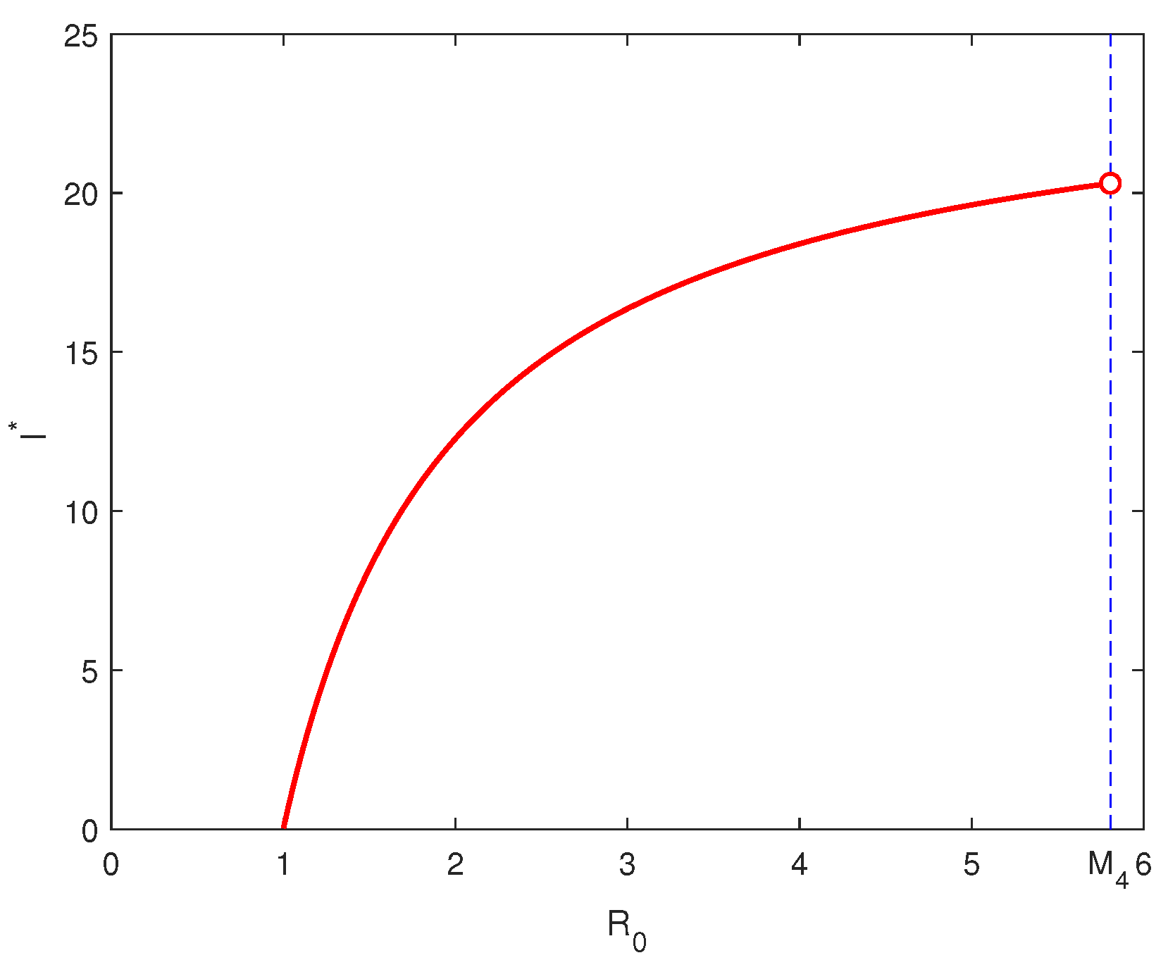
In the case where $R_0>1$, the existence of a rumor-endemic equilibrium is determined by the negativity of $M_1$. As a consequence, there exists a conditional forward bifurcation.

See Figure 1 for a schematic diagram of the conditional forward bifurcation of model (2).

4. Dynamics of the Rumor-Free Equilibrium

This section is devoted to the research of the asymptotic stability of the rumor-free equilibrium.

4.1. Local Asymptotic Stability

The linearized system of model (2) at $E_0=(0,0)$ is as follows:

$$\left\{\begin{array}{cc}\hfill {\displaystyle \frac{dx\left(t\right)}{dt}}& =-\delta x\left(t\right)+\left({\displaystyle \frac{\beta \mu }{\delta }}-{\gamma }_1\right)x(t-\tau ),\hfill \\ \hfill {\displaystyle \frac{dy\left(t\right)}{dt}}& ={\gamma }_{1}x(t-\tau )-\delta y\left(t\right).\hfill \end{array}\right.$$

(27)

The characteristic equation for the system is the following:

$$(\lambda +\delta )\left(\lambda +\delta -\left({\displaystyle \frac{\beta \mu }{\delta }}-{\gamma }_1\right)e^{-\lambda \tau }\right)=0.$$

(28)

Theorem 4.

Consider model (2) with no time delay. The following claims hold:

(1) 

Suppose $R_0<1$. Then, $E_0$ is locally asymptotically stable.

(2) 

Suppose $R_0>1$. Then, $E_0$ is unstable.

Proof of Theorem 4.

In this case, Equation (28) admits the negative root $-\delta$ and the root $({\gamma }_1+\delta )(R_0-1)$, which is negative or positive as $R_0<1$ or $R_0>1$. The claims follow from the Lyapunov stability theorem. □

Theorem 5.

Consider model (2) with a time delay. The following claims hold:

(1) 

Suppose $R_0<1$ and ${\displaystyle \frac{\beta \mu }{\delta }}+\delta \ge {\gamma }_1$. Then, $E_0$ is locally asymptotically stable.

(2) 

Suppose $R_0>1$. Then, $E_0$ is unstable.

Proof of Theorem 5.

Equation (28) admits the negative root $-\delta$. Let

$$P\left(\lambda \right)=\lambda +\delta -\left({\displaystyle \frac{\beta \mu }{\delta }}-{\gamma }_1\right)e^{-\lambda \tau }.$$

(29)

Two possibilities are distinguished.

Case 1: $R_0>1$. Then, $P\left(0\right)=({\gamma }_1+\delta )(1-R_0)<0$ and ${lim}_{\lambda \to +\infty }P\left(\lambda \right)=+\infty$. It follows from the continuity of $P\left(\lambda \right)$ that $P\left(\lambda \right)$ admits a positive zero. Hence, $E_0$ is unstable.

Case 2: $R_0<1$. Then, $P\left(0\right)=({\gamma }_1+\delta )(1-R_0)>0$ and ${lim}_{\lambda \to +\infty }P\left(\lambda \right)=+\infty$. In the case where ${\displaystyle \frac{\beta \mu }{\delta }}>{\gamma }_1$, it follows that $P^{\prime }\left(\lambda \right)=1+\left({\displaystyle \frac{\beta \mu }{\delta }}-{\gamma }_1\right)\tau e^{-\lambda \tau }>0$. So, $P\left(\lambda \right)$ is increasing on $[0,+\infty )$. Hence, $P\left(\lambda \right)$ admits no non-negative zero. In the case where ${\displaystyle \frac{\beta \mu }{\delta }}<{\gamma }_1$, it follows that $P\left(\lambda \right)>0$. Hence, $P\left(\lambda \right)$ admits no non-negative zero. In a word, $P\left(\lambda \right)$ admits no non-negative zero. Hence, if $P\left(\lambda \right)$ admits a zero with a positive real part, the zero must be complex and can be derived from a pair of complex conjugate zeros that cross the imaginary axis, denoted as $\pm i\omega$ ($\omega >0$) [52]. This implies the following:

$$P\left(i\omega \right)=i\omega +\delta -\left({\displaystyle \frac{\beta \mu }{\delta }}-{\gamma }_1\right)e^{-i\omega \tau }=0.$$

(30)

At this point, the method presented in [53] is used. Separating the real and imaginary parts, we obtain the following:

$$\left\{\begin{array}{cc}\hfill \left({\displaystyle \frac{\beta \mu }{\delta }}-{\gamma }_1\right)cos\left(\omega \tau \right)& =\delta ,\hfill \\ \hfill \left({\displaystyle \frac{\beta \mu }{\delta }}-{\gamma }_1\right)sin\left(\omega \tau \right)& =-\omega .\hfill \end{array}\right.$$

(31)

Taking both sides of each of the two equations into account, summing up the two resulting equations, and carrying out simple algebraic calculations, the following holds:

$${\omega }^2=\left({\displaystyle \frac{\beta \mu }{\delta }}+\delta -{\gamma }_1\right)({\gamma }_1+\delta )(R_0-1).$$

(32)

This implies ${\displaystyle \frac{\beta \mu }{\delta }}+\delta <{\gamma }_1$. Then, a contradiction occurs. Hence, $P\left(\lambda \right)$ admits no complex zero with a non-negative real part. Combining the above discussions, $P\left(\lambda \right)$ admits no zero with a non-negative real part. It follows from the Hurwitz criterion that $E_0$ is locally asymptotically stable. □

4.2. Global Asymptotic Stability

Theorem 6.

Consider model (2) and suppose $\beta \mu \le {\delta }^2$. Then, $E_0$ is globally attractive.

Proof of Theorem 6.

Consider the following positive definite function:

$$U\left(t\right)=I\left(t\right)+R\left(t\right)+\delta {\int }_{t-\tau }^{t}I\left(s\right)ds.$$

(33)

Then,

$$\begin{array}{cc}\hfill & {\displaystyle \frac{dU\left(t\right)}{dt}}={\displaystyle \frac{d{U}_1\left(t\right)}{dt}}+{\displaystyle \frac{d{U}_2\left(t\right)}{dt}}\hfill \\ \hfill & =\beta \left({\displaystyle \frac{\mu }{\delta }}-I\left(t\right)-R\left(t\right)\right)I(t-\tau )-{\gamma }_{1}I(t-\tau )-{\gamma }_{2}I\left(t\right)R(t-\tau )-\delta I\left(t\right)+{\gamma }_{1}I(t-\tau )\hfill \\ \hfill & +{\gamma }_{2}I\left(t\right)R(t-\tau )-\delta R\left(t\right)+\delta I\left(t\right)-\delta I(t-\tau )\hfill \\ \hfill & =\beta \left({\displaystyle \frac{\mu }{\delta }}-I\left(t\right)-R\left(t\right)\right)I(t-\tau )-\delta R\left(t\right)-\delta I(t-\tau )\hfill \\ \hfill & \le \left({\displaystyle \frac{\beta \mu }{\delta }}-\delta \right)I(t-\tau )\le 0.\hfill \end{array}$$

(34)

Moreover, ${\displaystyle \frac{dU\left(t\right)}{dt}}=0$ if and only if $I\left(t\right)=R\left(t\right)=0$. It follows from LaSalle’s invariance principle that $E_0$ is globally attractive. □

Theorem 7.

Consider model (2) with no time delay and suppose $\beta \mu \le {\delta }^2$. Then, $E_0$ is globally asymptotically stable.

Proof of Theorem 7.

The claim follows by combining Theorem 4 with Theorem 6. □

Theorem 8.

Consider model (2) with a time delay and suppose ${\gamma }_1-\delta \le {\displaystyle \frac{\beta \mu }{\delta }}\le \delta$. Then, $E_0$ is globally asymptotically stable.

Proof of Theorem 8.

The claim follows by combining Theorem 5 with Theorem 6. □

5. Dynamics of a Rumor-Endemic Equilibrium

Theorem 3 shows that in the case where $R_0>1$, depending on the negativity of $M_1$, model (2) either admits no rumor-endemic equilibrium or admits the unique rumor-endemic equilibrium $E^{*}=(I^{*},R^{*})$. In what follows, assume $R_0>1$ and $M_1<0$. Hence, a rumor-endemic equilibrium $E^{*}$ exists.

The linearized system of model (2) at $E^{*}$ is as follows:

$$\left\{\begin{array}{cc}\hfill {\displaystyle \frac{dx\left(t\right)}{dt}}& =-(\delta +\beta I^{*}+{\gamma }_2{R}^{*})x\left(t\right)+\left({\displaystyle \frac{\beta \mu }{\delta }}-{\gamma }_1-\beta I^{*}-\beta R^{*}\right)x(t-\tau )-\beta I^{*}y\left(t\right)\hfill \\ \hfill & -{\gamma }_2{I}^{*}y(t-\tau ),\hfill \\ \hfill {\displaystyle \frac{dy\left(t\right)}{dt}}& ={\gamma }_2{R}^{*}x\left(t\right)+{\gamma }_{1}x(t-\tau )-\delta y\left(t\right)+{\gamma }_2{I}^{*}y(t-\tau ).\hfill \end{array}\right.$$

(35)

In view of Equation (12), the following holds:

$$\left\{\begin{array}{cc}\hfill {\displaystyle \frac{dx\left(t\right)}{dt}}& =-(\delta +\beta I^{*}+{\gamma }_2{R}^{*})x\left(t\right)+({\gamma }_2{R}^{*}+\delta )x(t-\tau )-\beta I^{*}y\left(t\right)-{\gamma }_2{I}^{*}y(t-\tau ),\hfill \\ \hfill {\displaystyle \frac{dy\left(t\right)}{dt}}& ={\gamma }_2{R}^{*}x\left(t\right)+{\gamma }_{1}x(t-\tau )-\delta y\left(t\right)+{\gamma }_2{I}^{*}y(t-\tau ).\hfill \end{array}\right.$$

(36)

The characteristic equation for the system is as follows:

$$\begin{array}{cc}\hfill Q\left(\lambda \right)& =(\lambda +(\delta +\beta I^{*}+{\gamma }_2{R}^{*})-({\gamma }_2{R}^{*}+\delta )e^{-\lambda \tau })(\lambda +\delta -{\gamma }_2{I}^{*}{e}^{-\lambda \tau })\hfill \\ \hfill & +(\beta I^{*}+{\gamma }_2{I}^{*}{e}^{-\lambda \tau })({\gamma }_2{R}^{*}+{\gamma }_1{e}^{-\lambda \tau })\hfill \\ \hfill & =0.\hfill \end{array}$$

(37)

Simplification yields the following:

$$Q\left(\lambda \right)={\lambda }^2+a_1\lambda +a_2+(a_3\lambda +a_4)e^{-\lambda \tau }+a_5{e}^{-2\lambda \tau }=0,$$

(38)

where

$$a_1=2\delta +\beta I^{*}+{\gamma }_2{R}^{*}>0,$$

(39)

$$a_2={\delta }^2+\beta \delta I^{*}+{\gamma }_2\delta R^{*}+\beta {\gamma }_2{I}^{*}{R}^{*}>0,$$

(40)

$$a_3=-(\delta +{\gamma }_2{I}^{*}+{\gamma }_2{R}^{*})<0,$$

(41)

$$a_4=-({\delta }^2+{\gamma }_2\delta I^{*}+{\gamma }_2\delta R^{*}+\beta {\gamma }_2{I}^{*2})+\beta {\gamma }_1{I}^{*},$$

(42)

$$a_5={\gamma }_2{I}^{*}({\gamma }_1+\delta +{\gamma }_2{R}^{*})>0.$$

(43)

Theorem 9.

Consider model (2) with no time delay. Suppose the following conditions are met:

(C1) 

$a_1+a_3>0$.

(C2) 

$a_2+a_4+a_5>0$.

Then, $E^{*}$ is locally asymptotically stable.

Proof of Theorem 9.

In this case, $Q\left(\lambda \right)={\lambda }^2+(a_1+a_3)\lambda +(a_2+a_4+a_5)$. By the Hurwitz criterion, $Q\left(\lambda \right)$ admits a pair of zeros with negative real parts. The claim follows from the Lyapunov stability theorem. □

Theorem 10.

Consider model (2) with a very small time delay. Let

$${\omega }_0=\sqrt{{\displaystyle \frac{\sqrt{{(a_1^2-2a_2-a_3^2)}^2+4{(a_4+a_5)}^2}-(a_1^2-2a_2-a_3^2)}{2}}}.$$

(44)

Suppose the following conditions are met:

(C1) 

$a_1+a_3\ge 0$.

(C2) 

Either $a_4>0$ or ($a_4\le 0$ ∧ $a_2+a_4>0$).

(C3) 

$\left|Q\right(i{\omega }_0\left)\right|$ is not very small.

Then, $E^{*}$ is locally asymptotically stable.

Proof of Theorem 10.

Generally speaking, it is difficult to show the local asymptotic stability of a rumor-endemic equilibrium in the presence of multiple time delays. Now, develop a novel approximate technique to deal with the local asymptotic stability of model (2) with a small time delay.

Since $a_1>0$, $a_2>0$, $a_5>0$, and $a_3<0$, we have the following:

$$Q\left(\lambda \right)\ge {\lambda }^2+(a_1+a_3)\lambda +a_2+a_4{e}^{-\lambda \tau },\lambda \ge 0.$$

(45)

Two possibilities are distinguished.

Case 1: $a_4\le 0$. Then, $Q\left(\lambda \right)\ge {\lambda }^2+(a_1+a_3)\lambda +(a_2+a_4)$. It follows from condition (C1) and the second part of condition (C2) that $Q\left(\lambda \right)>0$ for all $\lambda \ge 0$.

Case 2: $a_4>0$. Then, $Q\left(\lambda \right)\ge {\lambda }^2+(a_1+a_3)\lambda +a_2$. It follows from assumption (C1) and the first part of condition (C2) that $Q\left(\lambda \right)>0$ for all $\lambda \ge 0$.

By combining these discussions, it follows that $Q\left(\lambda \right)$ admits no non-negative zero. Suppose $Q\left(\lambda \right)$ admits a zero with a positive real part. Then, the zero is complex and admits a nonzero imaginary part. This implies $Q\left(\lambda \right)$ admits a pair of purely imaginary zeros, denoted $\pm i\omega$ ($\omega >0$). Hence,

$$\begin{array}{cc}\hfill Q\left(i\omega \right)& ={\left(i\omega \right)}^2+i{a}_1\omega +a_2+(i{a}_3\omega +a_4)e^{-i\omega \tau }+a_5{e}^{-2i\omega \tau }\hfill \\ \hfill & =-{\omega }^2+i{a}_1\omega +a_2+(i{a}_3\omega +a_4)(cos\left(\omega \tau \right)-isin\left(\omega \tau \right))\hfill \\ \hfill & +a_5(cos\left(2\omega \tau \right)-isin\left(2\omega \tau \right))\hfill \\ \hfill & =(-{\omega }^2+a_2+a_3\omega sin\left(\omega \tau \right)+a_{4}cos\left(\omega \tau \right)+a_{5}cos\left(2\omega \tau \right))\hfill \\ \hfill & +i(a_1\omega +a_3\omega cos\left(\omega \tau \right)-a_{4}sin\left(\omega \tau \right)-a_{5}sin\left(2\omega \tau \right))\hfill \\ \hfill & =0.\hfill \end{array}$$

(46)

Separating the real and imaginary parts, it follows that

$$\left\{\begin{array}{cc}\hfill a_3\omega sin\left(\omega \tau \right)+a_{4}cos\left(\omega \tau \right)+a_{5}cos\left(2\omega \tau \right)& ={\omega }^2-a_2,\hfill \\ \hfill a_3\omega cos\left(\omega \tau \right)-a_{4}sin\left(\omega \tau \right)-a_{5}sin\left(2\omega \tau \right)& =-a_1\omega .\hfill \end{array}\right.$$

(47)

Taking both sides of each of the two equations into account, summing them, and carrying out algebraic calculations, it follows that

$$a_3^2{\omega }^2+a_4^2+a_5^2-2a_3{a}_5\omega sin\left(\omega \tau \right)+2a_4{a}_{5}cos\left(\omega \tau \right)={({\omega }^2-a_2)}^2+{\left(a_1\omega \right)}^2.$$

(48)

$sin\left(\omega \tau \right)\approx 0$ and $cos\left(\omega \tau \right)\approx 1$ follow from the assumption that $\tau$ is very small. So,

$$a_3^2{\omega }^2+a_4^2+a_5^2+2a_4{a}_5\approx {({\omega }^2-a_2)}^2+{\left(a_1\omega \right)}^2.$$

(49)

Simplifying, it follows that

$$R\left(\omega \right)={\omega }^4+(a_1^2-2a_2-a_3^2){\omega }^2-{(a_4+a_5)}^2\approx 0.$$

(50)

Let $z={\omega }^2$. Then,

$$R\left(z\right)=z^2+(a_1^2-2a_2-a_3^2)z-{(a_4+a_5)}^2.$$

(51)

So,

$$\omega \approx \sqrt{{\displaystyle \frac{\sqrt{{(a_1^2-2a_2-a_3^2)}^2+4{(a_4+a_5)}^2}-(a_1^2-2a_2-a_3^2)}{2}}}={\omega }_0.$$

(52)

Hence, $\left|Q\right(i{\omega }_0\left)\right|$ is very small. Then, a contradiction occurs. Therefore, $Q\left(\lambda \right)$ admits no complex zero with a non-negative real part. The claim follows from the Lyapunov stability theorem. □

Remark 1.

Condition (C3) of Theorem 10 is less conservative.

Remark 2.

It is seen from Theorems 9 and 10 that the local asymptotic stability of $E^{*}$ is determined by five quantities, $a_1$, $a_2$, $a_3$, $a_4$, and $a_5$, as well as the size of $\left|Q\right(i{\omega }_0\left)\right|$. Hence, it is difficult to use a plot to exhibit the stability transition of a rumor-endemic equilibrium for model (2).

Remark 3.

By employing the developed technique, the local asymptotic stability of the rumor-endemic equilibrium of model (2) in the presence of a small delay has been proven successfully. After preliminary research, it was found that the technique can be used to prove the local asymptotic stability of a rumor-endemic equilibrium of some rumor-spreading models with multiple distinct time delays. Related research is ongoing.

6. Simulation Experiments

In the preceding sections, some theoretical results are reported. This section is dedicated to the verification of these results through simulation experiments.

6.1. Asymptotic Stability of the Rumor-Free Equilibrium

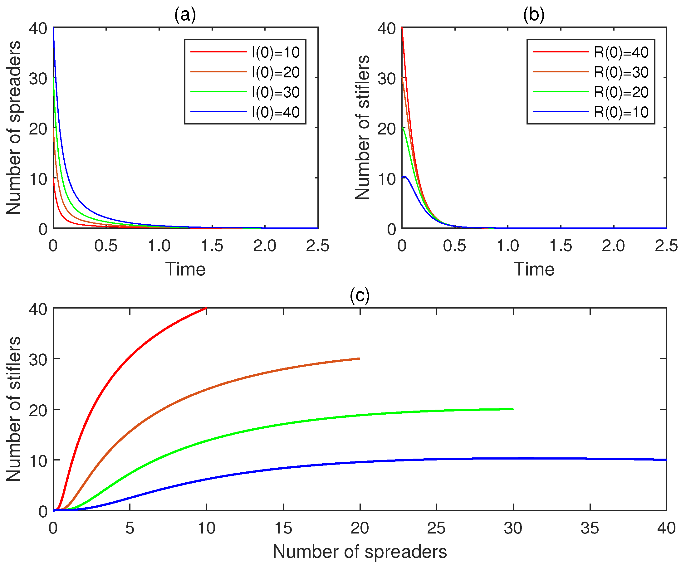
• Experiment 1: Consider model (2) with no time delay, where $\mu =500$, $\delta =10$, $\beta =0.15$, ${\gamma }_1=0.25$, and ${\gamma }_2=0.3$. Since $R_0<1$, it follows from claim (1) of Theorem 3 that the rumor-free equilibrium $E_0$ is locally asymptotically stable. Let $\left(I\right(0),R(0\left)\right)\in \left\{\right(10,40),(20,30),(30,20),(40,10\left)\right\}$. Figure 2a displays the time plot for the number of spreaders. Figure 2b exhibits the time plot for the number of stiflers. Figure 2c plots the phase portrait for the state evolution. It is seen that $E_0$ is locally asymptotically stable.
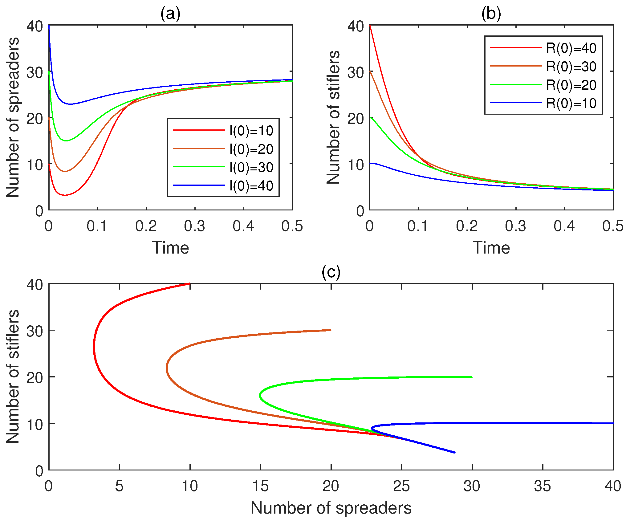
• Experiment 2: Consider model (2) with no time delay, where $\mu =500$, $\delta =10$, $\beta =0.3$, ${\gamma }_1=0.25$, and ${\gamma }_2=0.3$. Since $R_0>1$, it follows from claim (2) of Theorem 3 that the rumor-free equilibrium $E_0$ is unstable. Let $\left(I\right(0),R(0\left)\right)\in \left\{\right(10,40),(20,30),(30,20),(40,10\left)\right\}$. Figure 3a demonstrates the time plot for the number of spreaders. Figure 3b presents the time plot for the number of stiflers. Figure 3c portrays the phase portrait for the state transition. It is seen that $E_0$ is unstable.
• Experiment 3: Consider model (2) with a time delay, where $\mu =500$, $\delta =10$, $\beta =0.15$, ${\gamma }_1=0.25$, ${\gamma }_2=0.3$, and $\tau =0.5$. Since $R_0<1$ and $\beta \mu <{\delta }^2$, it follows from claim (1) of Theorem 4 that the rumor-free equilibrium $E_0$ is locally asymptotically stable. For $-\tau \le \theta \le 0$, let $\left(I\right(\theta ),R(\theta \left)\right)\equiv (10,40)$, $(20,30)$, or $(30,20)$ or $(40,10)$. Figure 4a depicts the time plot for the number of spreaders. Figure 4b provides the time plot for the number of stiflers. Figure 4c shows the phase portrait for the state transition. It is seen that $E_0$ is locally asymptotically stable.
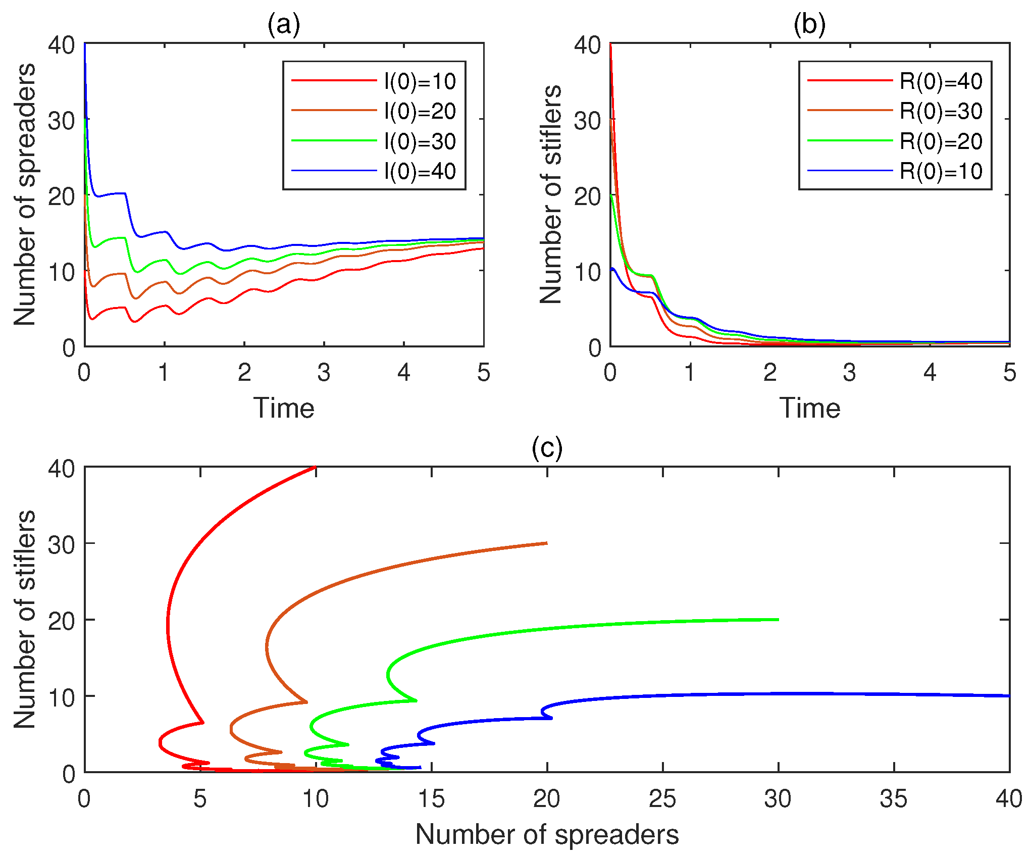
• Experiment 4: Consider model (2) with a time delay, where $\mu =500$, $\delta =10$, $\beta =0.3$, ${\gamma }_1=0.25$, ${\gamma }_2=0.3$, and $\tau =0.5$. Since $R_0>1$, it follows from claim (2) of Theorem 4 that the rumor-free equilibrium $E_0$ is unstable. For $-\tau \le \theta \le 0$, let $\left(I\right(\theta ),R(\theta \left)\right)\equiv (10,40)$, $(20,30)$, $(30,20)$, or $(40,10)$. Figure 5a exhibits the time plot for the number of spreaders. Figure 5b displays the time plot for the number of stiflers. Figure 5c plots the phase portrait for the state transition. It is seen that $E_0$ is unstable.
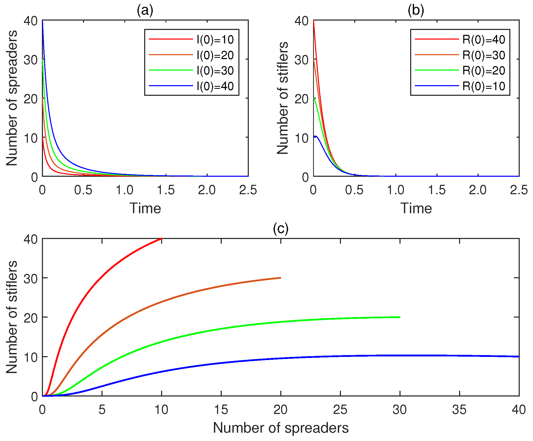
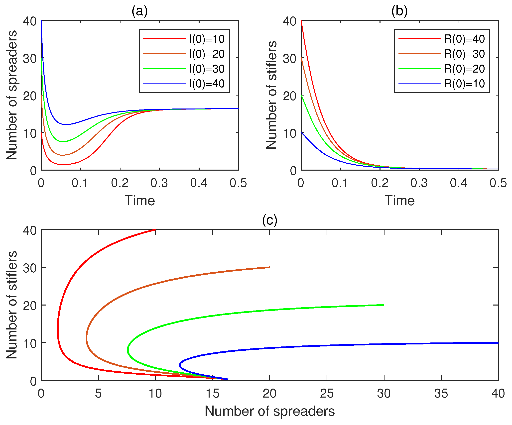
• Experiment 5: Consider model (2) with no time delay, where $\mu =500$, $\delta =10$, $\beta =0.15$, ${\gamma }_1=0.25$, and ${\gamma }_2=3$. Since $\beta \mu <{\delta }^2$, it follows from Theorem 6 that the rumor-free equilibrium $E_0$ is globally asymptotically stable. Let $\left(I\right(0),R(0\left)\right)\in \left\{\right(10,40),(20,30),(30,20),(40,10\left)\right\}$. Figure 6a depicts the time plot for the number of spreaders. Figure 6b shows the time plot for the number of stiflers. Figure 6c exhibits the phase portrait for the state transition. It is seen that $E_0$ is globally asymptotically stable.
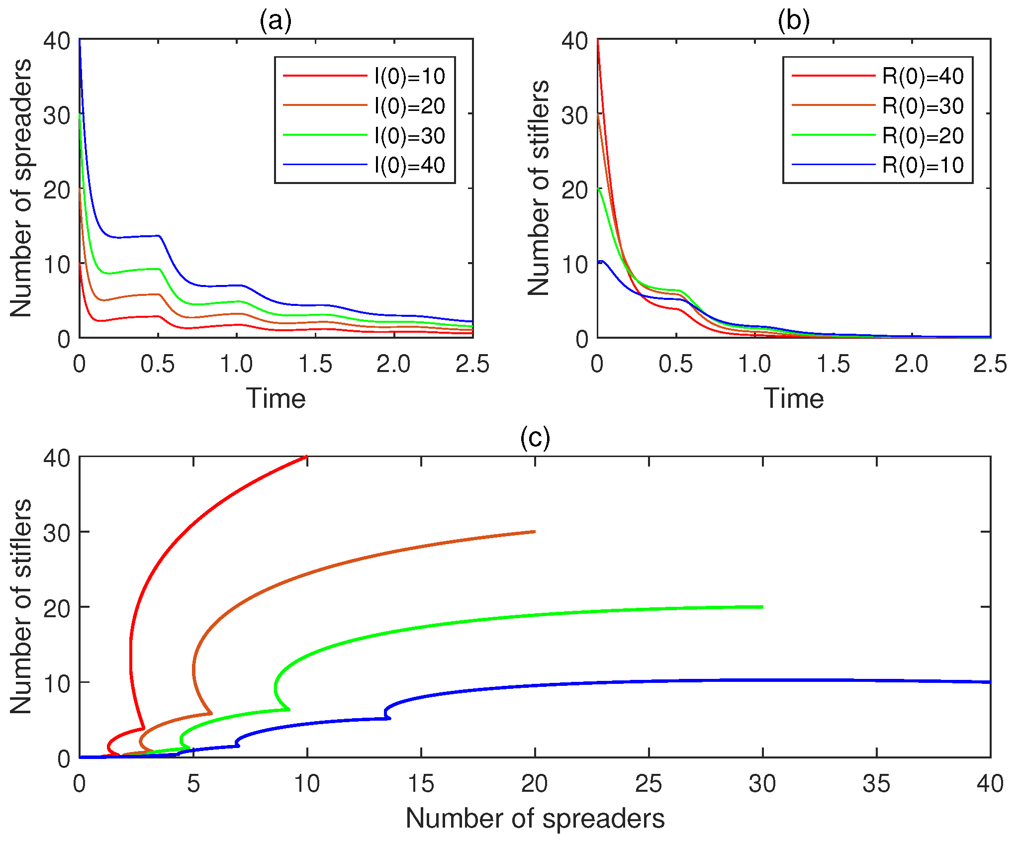
• Experiment 6: Consider model (2) with a time delay, where $\mu =500$, $\delta =10$, $\beta =0.15$, ${\gamma }_1=0.25$, ${\gamma }_2=0.3$, and $\tau =0.5$. Since ${\gamma }_1-\delta <{\displaystyle \frac{\beta \mu }{\delta }}<\delta$, it follows from Theorem 7 that the rumor-free equilibrium $E_0$ is globally asymptotically stable. For $-\tau \le \theta \le 0$, let $\left(I\right(\theta ),R(\theta \left)\right)\equiv (10,40)$, $(20,30)$, $(30,20)$, or $(40,10)$. Figure 7a provides the time plot for the number of spreaders. Figure 7b depicts the time plot for the number of stiflers. Figure 7c demonstrates the phase portrait for the state transition. It is seen that $E_0$ is globally asymptotically stable.

6.2. Asymptotic Stability of a Rumor-Endemic Equilibrium

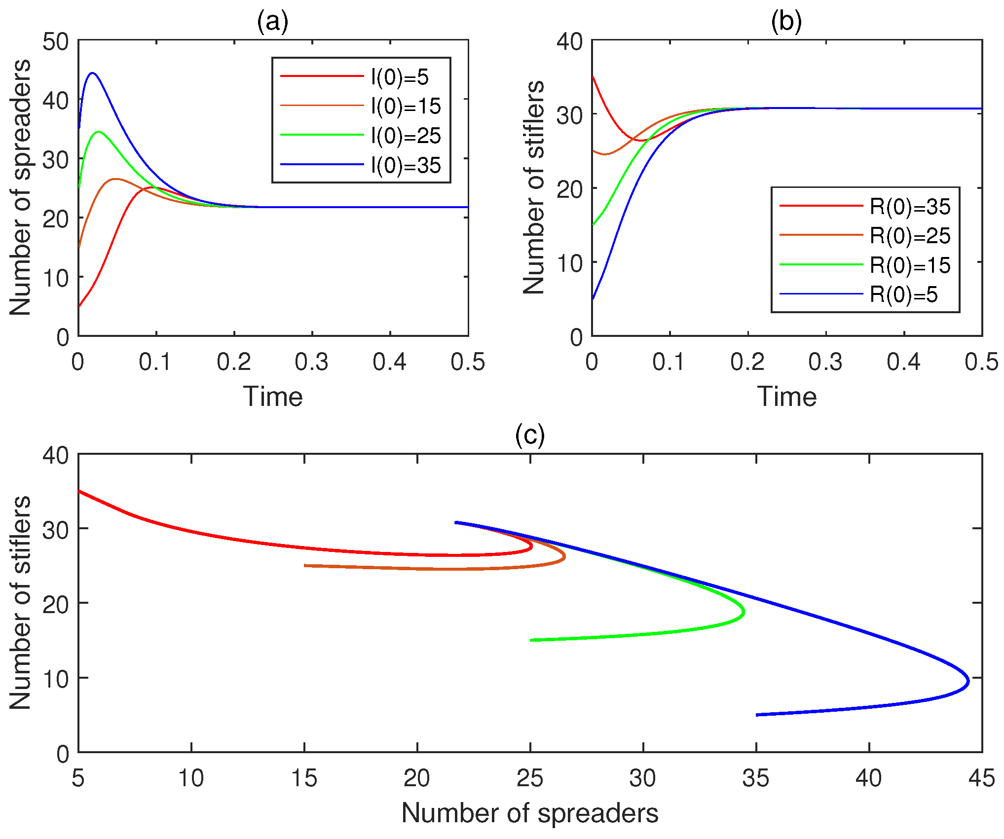
• Experiment 7: Consider model (5) with no time delay, where $\mu =472$, $\delta =20$, $\beta =2.43$, ${\gamma }_1=0.27$, and ${\gamma }_2=0.41$. Then, $E_2^{*}=(14.9193,0.2902)$ is a rumor-endemic equilibrium. Since $a_1+a_3>0$ and $a_2+a_4+a_5>0$, it follows from Theorem 8 that $E_2^{*}$ is locally asymptotically stable. Let $\left(I\right(0),R(0\left)\right)\in \left\{\right(10,40),(20,30),(30,20),(40,10\left)\right\}$. Figure 8a displays the time plot for the number of spreaders. Figure 8b exhibits the time plots for the number of stiflers. Figure 8c plots the phase portrait for the state transition. It is seen that $E_2^{*}$ is locally asymptotically stable.
• Experiment 8: Consider model (2) with a small time delay, where $\mu =600$, $\delta =10$, $\beta =3.2$, ${\gamma }_1=8$, ${\gamma }_2=0.2$, and $\tau =0.01$. Then, $E_2^{*}=(21.7237,30.7306)$ is a rumor-endemic equilibrium. Since $a_1+a_3>0$, $a_4>0$, and $\left|Q\right(i{\omega }_0\left)\right|=1440.3016$, it follows from Theorem 9 that $E_2^{*}$ is locally asymptotically stable. For $-\tau \le \theta \le 0$, let $\left(I\right(\theta ),R(\theta \left)\right)\equiv (10,40)$, $(20,30)$, $(30,20)$, or $(40,10)$. Figure 9a provides the time plot for the number of spreaders. Figure 9b depicts the time plot for the number of stiflers. Figure 9c presents the phase portrait for the state transition. It is seen that $E_2^{*}$ is locally asymptotically stable.
• Experiment 9: Consider model (2) with a small time delay, where $\mu =560$, $\delta =15$, $\beta =3.5$, ${\gamma }_1=0.3$, ${\gamma }_2=0.44$, and $\tau =0.01$. Then, $E_2^{*}=(28.7917,3.7045)$ is a rumor-endemic equilibrium. Since $a_1+a_3>0$, $a_4\le 0$, $a_2+a_4>0$, and $\left|Q\right(i{\omega }_0\left)\right|=1516.5674$, it follows from Theorem 9 that $E_2^{*}$ is locally asymptotically stable. For $-\tau \le \theta \le 0$, let $\left(I\right(\theta ),R(\theta \left)\right)\equiv (10,40)$, $(20,30)$, $(30,20)$, or $(40,10)$. Figure 10a provides the time plot for the number of spreaders. Figure 10b depicts the time plot for the number of stiflers. Figure 10c presents the phase portrait for the state transition. It is seen that $E_2^{*}$ is locally asymptotically stable.

6.3. Effect of the Time Delay

Under model (2), the effect of the time delay on rumor spreading is examined through numerical simulations.

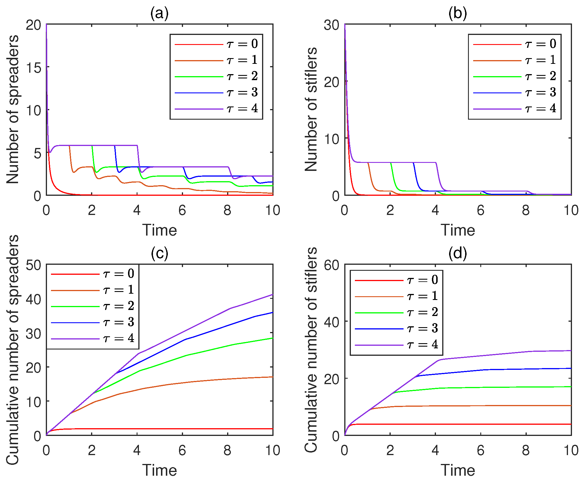
• Experiment 10: Consider five delayed rumor-spreading models, where $\mu =500$, $\delta =10$, $\beta =0.15$, ${\gamma }_1=0.25$, ${\gamma }_2=0.3$, and $\tau \in \{0,1,2,3,4\}$. For $-\tau \le \theta \le 0$, let $I\left(\theta \right)\equiv 10$ and $R\left(\theta \right))\equiv 40$. For each $\tau$, Figure 11a exhibits the time plot for the number of spreaders, Figure 11b depicts the time plot for the number of stiflers, Figure 11c displays the time plot for the cumulative number of spreaders, and Figure 11d shows the time plot for the cumulative number of stiflers. It is observed that with the increase in the time delay, the four numbers increase simultaneously.
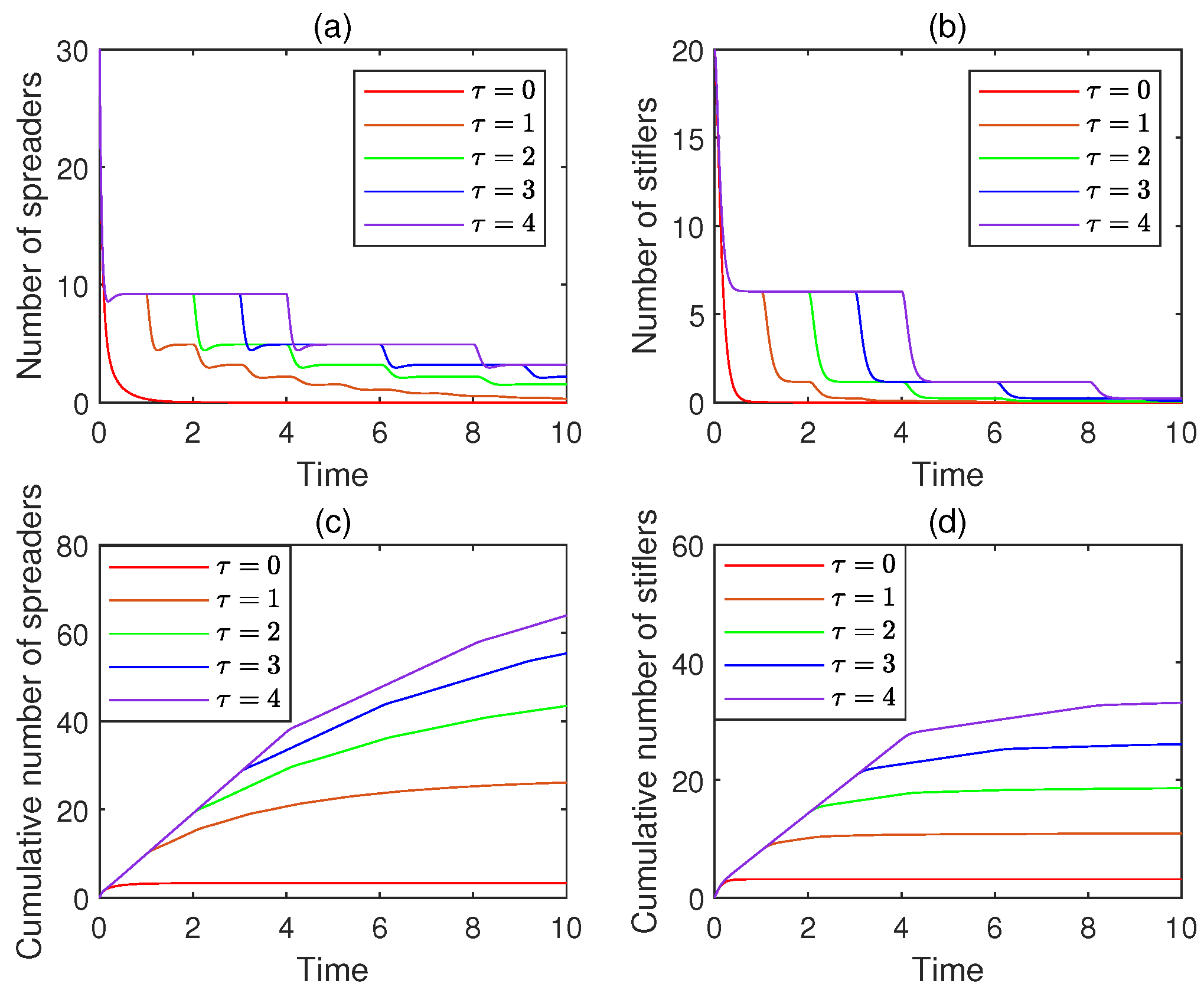
• Experiment 11: Consider five delayed rumor-spreading models, where $\mu =500$, $\delta =10$, $\beta =0.15$, ${\gamma }_1=0.25$, ${\gamma }_2=0.3$, and $\tau \in \{0,1,2,3,4\}$. For $-\tau \le \theta \le 0$, let $I\left(\theta \right)\equiv 20$ and $R\left(\theta \right))\equiv 30$. For each $\tau$, Figure 12a exhibits the time plot for the number of spreaders, Figure 12b depicts the time plot for the number of stiflers, Figure 12c displays the time plot for the cumulative number of spreaders, and Figure 12d shows the time plot for the cumulative number of stiflers. It is observed that with the increase in the time delay, the four numbers increase simultaneously.
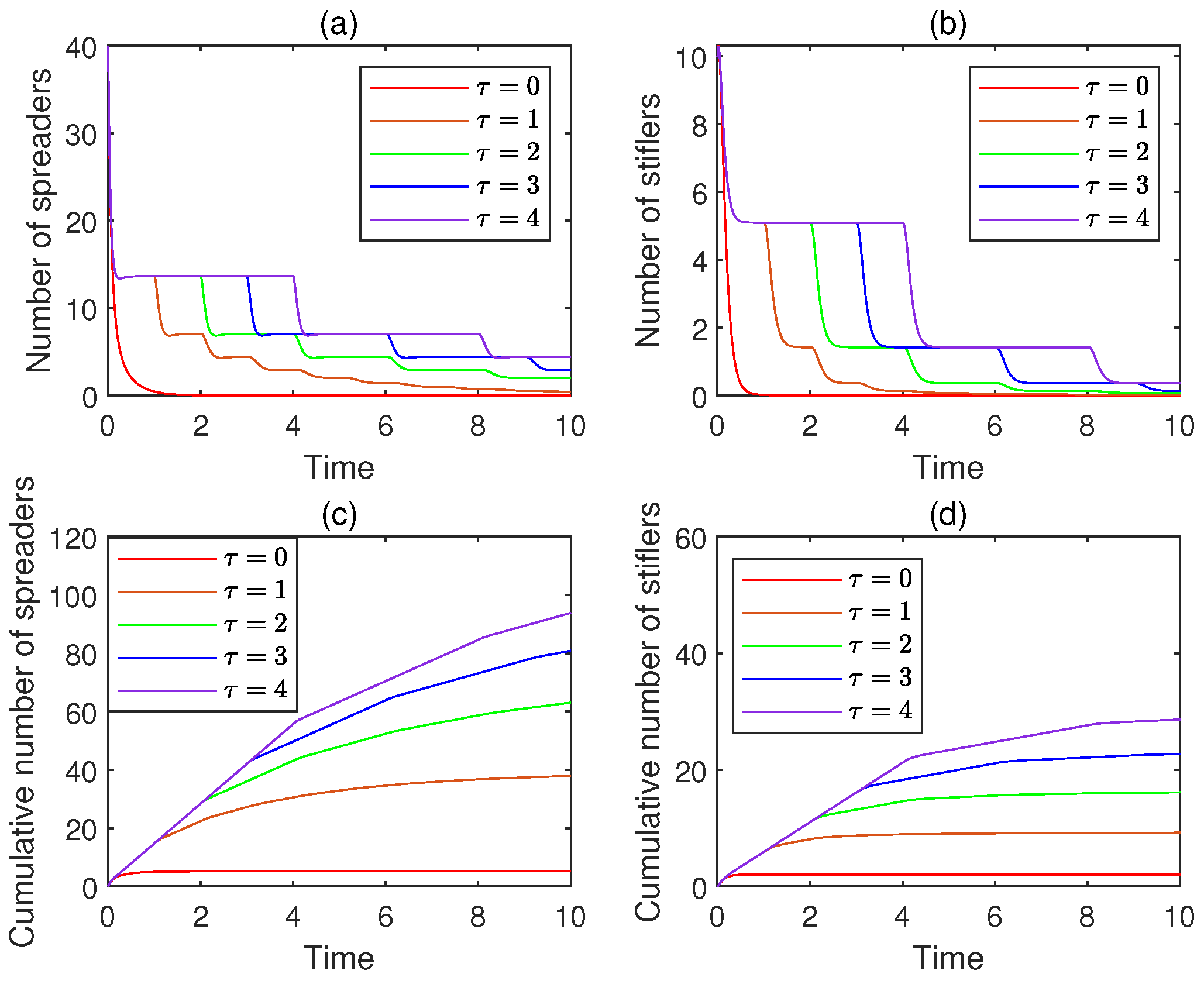
• Experiment 12: Consider five delayed rumor-spreading models, where $\mu =500$, $\delta =10$, $\beta =0.15$, ${\gamma }_1=0.25$, ${\gamma }_2=0.3$, and $\tau \in \{0,1,2,3,4\}$. For $-\tau \le \theta \le 0$, let $I\left(\theta \right)\equiv 30$ and $R\left(\theta \right))\equiv 20$. For each $\tau$, Figure 13a exhibits the time plot for the number of spreaders, Figure 13b depicts the time plot for the number of stiflers, Figure 13c displays the time plot for the cumulative number of spreaders, and Figure 13d shows the time plot for the cumulative number of stiflers. It is observed that with the increase in the time delay, the four numbers increase simultaneously.
• Experiment 13: Consider five delayed rumor-spreading models, where $\mu =500$, $\delta =10$, $\beta =0.15$, ${\gamma }_1=0.25$, ${\gamma }_2=0.3$, and $\tau \in \{0,1,2,3,4\}$. For $-\tau \le \theta \le 0$, let $I\left(\theta \right)\equiv 40$ and $R\left(\theta \right))\equiv 10$. For each $\tau$, Figure 14a exhibits the time plot for the number of spreaders, Figure 14b depicts the time plot for the number of stiflers, Figure 14c displays the time plot for the cumulative number of spreaders, and Figure 14d shows the time plot for the cumulative number of stiflers. It is observed that with the increase in the time delay, the four numbers increase simultaneously.

Based on the experimental results for the above four experiments and 1000 additional experiments, the following phenomena are observed:

(a)

With the increase in the time delay, the number of spreaders increases. Hence, it is concluded that the increase in the time delay facilitates rumor spreading and extends the rumor-spreading duration.

(b)

With the increase in the time delay, the cumulative number of spreaders, which is represented by the area under the number of spreaders, increases.

(c)

With the increase in the time delay, the number of stiflers increases. Hence, it is concluded that the increase in the time delay facilitates rumor stifling and extends the rumor-stifling duration.

(d)

With the increase in the time delay, the cumulative number of stiflers, which is represented by the area under the number of stiflers, increases.

(e)

Three identical time delays work collaboratively to change the rate of increase in spreaders.

7. Parameter Sensitivity and Implications

In this section, the effect of different parameters on the basic reproduction number is examined. Then, the relationship between the existence of a rumor-endemic equilibrium and the range of parameters is inspected.

7.1. Effect of the Parameters on the Basic Reproduction Number

It is seen from Equation (9) that the basic reproduction number is closely related to four parameters: $\mu$, $\delta$, $\beta$, and ${\gamma }_1$.

Theorem 11.

$R_0$ increases with the increase in μ and β. $R_0$ decreases with the increase in δ and ${\gamma }_1$.

Proof of Theorem 11.

$$\begin{array}{cc}\hfill {\displaystyle \frac{\partial R_0}{\partial \mu }}& ={\displaystyle \frac{\beta }{\delta ({\gamma }_1+\delta )}}>0,{\displaystyle \frac{\partial R_0}{\partial \delta }}={\displaystyle \frac{-\beta \mu ({\gamma }_1+2\delta )}{{\delta }^2{({\gamma }_1+\delta )}^2}}<0,\hfill \\ \hfill {\displaystyle \frac{\partial R_0}{\partial \beta }}& ={\displaystyle \frac{\mu }{\delta ({\gamma }_1+\delta )}}>0,{\displaystyle \frac{\partial R_0}{\partial {\gamma }_1}}={\displaystyle \frac{-\beta \mu }{\delta {({\gamma }_1+\delta )}^2}}<0.\hfill \end{array}$$

(53)

The claims hold. □

7.2. Relationship Between the Existence of a Rumor-Endemic Equilibrium and the Range of Some Parameters

Lemma 7.

Let

$$M_8={\displaystyle \frac{\delta ({\gamma }_2\delta -\beta {\gamma }_1-\beta \delta )}{\beta {\gamma }_2}},$$

(54)

$$M_9={\displaystyle \frac{{\gamma }_2{\delta }^2}{{\gamma }_2\mu +{\gamma }_1\delta +{\delta }^2}},$$

(55)

$$M_{10}={\displaystyle \frac{{\gamma }_2{\delta }^2-\beta {\gamma }_2\mu -\beta {\delta }^2}{\beta \delta }}.$$

(56)

The following claims hold:

(C1) 

$M_1>0\iff \mu <M_8$$\iff \beta <M_9$$\iff {\gamma }_1<M_{10}$.

(C2) 

$M_1<0\iff \mu >M_8$$\iff \beta >M_9$$\iff {\gamma }_1>M_{10}$.

(C3) 

$M_1=0\iff \mu =M_8$$\iff \beta =M_9$$\iff {\gamma }_1=M_{10}$.

Proof of Lemma 7.

The claims follow directly from Equation (10). □

Remark 4.

$M_8$ is independent of μ, $M_9$ is independent of β, and $M_{10}$ is independent of ${\gamma }_1$.

Lemma 8.

Let

$$M_{11}={\displaystyle \frac{\delta ({\gamma }_1+\delta )}{\beta }},M_{12}={\displaystyle \frac{\delta ({\gamma }_1+\delta )}{\mu }},M_{13}={\displaystyle \frac{\beta \mu -{\delta }^2}{\delta }}.$$

(57)

The following claims hold:

(C1) 

$R_0>1\iff \mu >M_{11}\iff \beta >M_{12}\iff {\gamma }_1<M_{13}$.

(C2) 

$R_0=1\iff \mu =M_{11}\iff \beta =M_{12}\iff {\gamma }_1=M_{13}$.

(C3) 

$R_0<1\iff \mu <M_{11}\iff \beta <M_{12}\iff {\gamma }_1>M_{13}$.

Proof of Lemma 8.

The claims follow directly from Equation (9). □

Remark 5.

$M_{11}$ is independent of μ, $M_{12}$ is independent of β, and $M_{13}$ is independent of ${\gamma }_1$.

Theorem 12.

Suppose $\mu \le M_{11}$, $\beta \le M_{12}$, or ${\gamma }_1\ge M_{13}$. Then, model (2) admits no rumor-endemic equilibrium.

Proof of Theorem 12.

The claim follows by combining claim (C1) of Theorem 3 with Lemma 8. □

This theorem provides three criteria for the nonexistence of a rumor-endemic equilibrium in terms of $\mu$, $\beta$, and ${\gamma }_1$.

Theorem 13.

Suppose one of the following conditions is met:

(C1) 

$M_{11}<\mu \le M_8$.

(C2) 

$M_{12}<\beta \le M_9$.

(C3) 

${\gamma }_1\le M_{10}$, ${\gamma }_1<M_{13}$.

Then, model (2) admits no rumor-endemic equilibrium.

Proof of Theorem 13.

The claim follows by combining claim (C2) of Theorem 3 with Lemmas 7 and 8. □

This theorem provides three criteria for the nonexistence of a rumor-endemic equilibrium in terms of $\mu$, $\beta$, and ${\gamma }_1$.

Theorem 14.

Suppose one of the following conditions is met:

(C1) 

$\mu >M_8$, $\mu >M_{11}$.

(C2) 

$\beta >M_9$, $\beta >M_{12}$.

(C3) 

$M_{10}<{\gamma }_1<M_{13}$.

Then, model (2) admits the rumor-endemic equilibrium $E^{*}$.

Proof of Theorem 14.

The claim follows by combining claim (C3) of Theorem 3 with Lemmas 7 and 8. □

This theorem provides three criteria for the existence of a rumor-endemic equilibrium $E^{*}$ in terms of $\mu$, $\beta$, and ${\gamma }_1$, respectively.

8. Conclusions

In this article, a rumor-spreading model with three identical time delays is introduced. A local forward bifurcation phenomenon is observed, which is of particular interest. A collection of criteria for the local and global asymptotic stability of the rumor-free equilibrium is provided. A novel technique of dealing with small time delays is suggested. Building on this, a criterion for the local asymptotic stability of the rumor-endemic equilibrium is presented. The relationship of the rumor-endemic equilibrium with the parameters is examined. This work takes a critical step toward understanding the dynamics of rumor-spreading models with time delays.

Several related issues warrant further investigation. First, to our knowledge, although there are several publicly available rumor datasets [54,55], to date, there is no publicly available rumor-spreading-related dataset, not to mention a delayed rumor-spreading-related dataset. From our perspective, the key to justifying a delayed rumor-spreading model is to gather and analyze huge volumes of data about delayed rumor spreading, which is a challenging task. Second, this article considers a rumor-spreading model with three identical time delays. In real-world applications, a rumor-spreading model with multiple distinct time delays may be used to characterize the spreading process of a rumor more accurately. Hence, it is worthwhile to introduce rumor-spreading models with multiple distinct time delays. Thirdly, this article considers a rumor-spreading model with a constant time delay. In practice, a distributed or state-dependent delay is the general case, whereas a constant delay is a special case. Possibly owing to the inherent difficulty of studying the general case, there is no report in the literature on rumor-spreading models with distributed time delays or state-dependent time delays. This is an issue to be addressed. Next, optimal impulsive control theory is an important branch of optimal control theory, which has witnessed widespread applications [56,57]. Through optimal impulsive control, accurate and low-cost control can be achieved. Although the control problem of rumor spreading has been studied extensively through the optimal control approach [14,39,40,58], fewer studies on the optimal impulsive control of rumor spreading has been carried out [59]. From our perspective, accurate and low-cost control of rumor spreading should be achieved. Last, since the interaction between rumor spreading and rumor stifling is essentially a non-cooperative game [60], it is worth studying a delayed rumor-spreading model in the framework of game theory [18].

References

- Peterson, W.; Gist, N.P. Rumor and public opinion. Am. J. Sociol. 1951, 57, 159–167. [Google Scholar] [CrossRef]
- Allport, G.W.; Postman, L. An analysis of rumor. Public Opin. Q. 1946, 10, 501–517. [Google Scholar] [CrossRef]
- Britton, N.F. Essential Mathematical Biology; Springer: Berlin/Heidelberg, Germany, 2003. [Google Scholar]
- Goffman, W.; Newill, V.A. Generalization of epidemic Theory: An application to the transmission of ideas. Nature 1964, 204, 501–517. [Google Scholar] [CrossRef]
- Daley, D.J.; Kendall, D.G. Epidemics and rumours. Nature 1964, 204, 1118. [Google Scholar] [CrossRef]
- Daley, D.J.; Kendall, D.G. Stochastic rumours. IMA J. Appl. Math. 1965, 1, 42–55. [Google Scholar] [CrossRef]
- Zhao, L.; Wang, J.; Chen, Y.; Wang, Q.; Cheng, J.; Cui, H. SIHR rumor spreading model in social networks. Phys. A Stat. Mech. Its Appl. 2012, 391, 2444–2453. [Google Scholar] [CrossRef]
- Wang, J.; Zhao, L.; Huang, R. 2SI2R rumor spreading model in homogeneous networks. Phys. A Stat. Mech. Its Appl. 2014, 413, 153–161. [Google Scholar] [CrossRef]
- Zhao, L.; Wang, X.; Wang, J.; Qiu, X.; Xie, W. Rumor-propagation model with consideration of refutation mechanism in homogeneous social networks. Discret. Dyn. Nat. Soc. 2014, 1, 659273. [Google Scholar] [CrossRef]
- Wei, Y.; Huo, L.; He, H. Research on rumor-spreading model with Holling type III functional response. Mathematics 2022, 10, 632. [Google Scholar] [CrossRef]
- Huo, L.; Ding, F.; Liu, C.; Cheng, Y. Dynamical analysis of rumor spreading model considering node activity in complex networks. Complexity 2018, 1, 1049805. [Google Scholar] [CrossRef]
- Huo, L.; Chen, S. Rumor propagation model with consideration of scientific knowledge level and social reinforcement in heterogeneous network. Physica 2020, 559, 125063. [Google Scholar] [CrossRef]
- Huo, L.; Chen, S.; Xie, X.; Liu, H.; He, J. Optimal control of ISTR rumor propagation model with social reinforcement in heterogeneous network. Complexity 2021, 1, 5682543. [Google Scholar] [CrossRef]
- Tong, X.; Jiang, H.; Chen, X.; Yu, S.; Li, J. Dynamic analysis and optimal control of rumor spreading model with recurrence and individual behaviors in heterogeneous networks. Entropy 2022, 24, 464. [Google Scholar] [CrossRef]
- Yang, L.X.; Li, P.; Yang, X.; Wu, Y.; Tang, Y.Y. On the competition of two conflicting messages. Nonlinear Dyn. 2018, 91, 1853–1869. [Google Scholar] [CrossRef]
- Yang, L.X.; Zhang, T.; Yang, X.; Wu, Y.; Tang, Y.Y. Effectiveness analysis of a mixed rumor-quelling strategy. J. Frankl. Inst. 2018, 355, 8079–8105. [Google Scholar] [CrossRef]
- Zhao, J.; Yang, L.X.; Zhong, X.; Yang, X.; Wu, Y.; Tang, Y.Y. Minimizing the impact of a rumor via isolation and conversion. Physica 2019, 526, 120867. [Google Scholar] [CrossRef]
- Huang, D.W.; Yang, L.X.; Li, P.; Yang, X.; Tang, Y.Y. Developing cost-effective rumor-refuting strategy through game-theoretic approach. IEEE Syst. J. 2021, 15, 5034–5045. [Google Scholar] [CrossRef]
- Liu, F.; Liu, H.; Li, Y.; Sidorov, D. Two relaxed quadratic function negative-determination lemmas: Application to time-delay systems. Automatica 2023, 147, 110697. [Google Scholar] [CrossRef]
- Wu, M.; He, Y.; She, J.H.; Liu, G.P. Delay-dependent criteria for robust stability of time-varying delay systems. Automatica 2004, 40, 1435–1439. [Google Scholar] [CrossRef]
- Dey, R.; Ghosh, S.; Ray, G.; Rakshit, A.; Balas, V.E. Improved delay-range-dependent stability analysis of a time-delay system with norm bounded uncertainty. ISA Trans. 2015, 58, 50–57. [Google Scholar] [CrossRef]
- Sun, Y.; Li, N.; Shen, M.; Wei, Z.; Sun, G. Robust H∞ control of uncertain linear system with interval time-varying delay by using Wirtinger inequality. Appl. Math. Comput. 2018, 335, 1–11. [Google Scholar] [CrossRef]
- Wang, Y.; Liu, H.; Li, X. A novel method for stability analysis of time-varying delay systems. IEEE Trans. Autom. Control 2020, 66, 1422–1428. [Google Scholar] [CrossRef]
- He, Y.; Wang, Q.G.; Lin, C.; Wu, M. Augmented Lyapunov functional and delay-dependent stability for neural systems. Int. J. Robust Nonlinear Control 2005, 15, 923–933. [Google Scholar] [CrossRef]
- Li, Y.; Gu, K.; Zhou, J.; Xu, S. Estimating stable delay intervals with a discretized Lyapunov-Krasovskii functional formulation. Automatica 2014, 50, 1691–1697. [Google Scholar] [CrossRef]
- Seuret, A.; Gouaisbaut, F. Wirtinger-based integral inequality: Application to time-delay systems. Automatica 2013, 49, 2860–2866. [Google Scholar] [CrossRef]
- Lee, W.I.; Lee, S.Y.; Park, P. Affine Bessel-Legendre inequality: Application to stability analysis for systems with time-varying delays. Automatica 2018, 93, 535–539. [Google Scholar] [CrossRef]
- Zeng, H.B.; Liu, X.G.; Wang, W. A generalized free-matrix-based inequality for stability analysis of time-varying delay systems. Appl. Math. Comput. 2019, 354, 1–8. [Google Scholar] [CrossRef]
- Datta, R.; Dey, R.; Bhattacharya, B.; Saravanakumar, R.; Ahn, C.K. New double integral inequality with application to stability analysis for linear retarded systems. IET Control Theory Appl. 2019, 13, 1514–1524. [Google Scholar] [CrossRef]
- Park, P.; Ko, J.W.; Jeong, C. Reciprocally convex approach to stability of systems with time-varying delays. Automatica 2011, 47, 235–238. [Google Scholar] [CrossRef]
- Zhang, X.M.; Han, Q.L.; Seuret, A.; Gouaisbaut, F. An improved reciprocally convex inequality and an augmented Lyapunov-Krasovskii functional for stability of linear systems with time-varying delay. Automatica 2017, 84, 221–226. [Google Scholar] [CrossRef]
- Zhu, L.; Zhao, H. Dynamical behaviours and control measures of rumour-spreading model with consideration of network topology. Int. J. Syst. Sci. 2019, 48, 2064–2078. [Google Scholar] [CrossRef]
- Zhu, L.; Guan, G. Dynamical analysis of a rumor spreading model with self-discrimination and time delay in complex networks. Phys. A Stat. Mech. Its Appl. 2019, 533, 121953. [Google Scholar] [CrossRef]
- Zhu, L.; Liu, W.; Zhang, Z. Delay differential equations modeling of rumor propagation in both homogeneous and heterogeneous networks with a forced silence function. Appl. Math. Comput. 2020, 370, 124925. [Google Scholar] [CrossRef]
- Zhu, L.; Zhou, M.; Zhang, Z. Dynamical analysis and control strategies of rumor spreading models in both homogeneous and heterogeneous networks. J. Nonlinear Sci. 2020, 30, 2545–2576. [Google Scholar] [CrossRef]
- Cheng, Y.; Huo, L.; Zhao, L. Dynamical behaviors and control measures of rumor-spreading model in consideration of the infected media and time delay. Inf. Sci. 2021, 564, 237–253. [Google Scholar] [CrossRef]
- Cao, B.; Guan, G.; Shen, S.; Zhu, L. Dynamical behaviors of a delayed SIR information propagation model with forced silence function and control measures in complex networks. Eur. Phys. J. Plus 2023, 138, 402. [Google Scholar] [CrossRef]
- Ma, Y.; Xie, L.; Liu, S.; Chu, X. Dynamical behaviors and event-triggered impulsive control of a delayed information propagation model based on public sentiment and forced silence. Eur. Phys. J. Plus 2023, 138, 979. [Google Scholar] [CrossRef]
- Ding, N.; Guan, G.; Shen, S.; Zhu, L. Dynamical behaviors and optimal control of delayed S2IS rumor propagation model with saturated conversion function over complex networks. Commun. Nonlinear Sci. Numer. Simul. 2024, 128, 107603. [Google Scholar] [CrossRef]
- Luo, X.; Jiang, H.; Li, J.; Chen, S.; Xia, Y. Modeling and controlling delayed rumor propagation with general incidence in heterogeneous networks. Int. J. Mod. Phys. C 2024, 35, 2450020. [Google Scholar] [CrossRef]
- Ghosh, M.; Das, P. Analysis of online misinformation spread model incorporating external noise and time delay and control of media effort. Differ. Equ. Dyn. Syst. 2025, 33, 261–301. [Google Scholar] [CrossRef]
- Ghosh, M.; Das, S.; Das, P. Dynamics and control of delayed rumor propagation through social networks. J. Appl. Math. Comput. 2022, 68, 3011–3040. [Google Scholar] [CrossRef] [PubMed]
- Cheng, Y.; Huo, L.; Zhao, L. Stability analysis and optimal control of rumor spreading model under media coverage considering time delay and pulse vaccination. Chaos Solitons Fractals 2022, 157, 111931. [Google Scholar] [CrossRef]
- Huo, L.; Chen, X. Dynamical analysis of a stochastic rumor-spreading model with Holling II functional response function and time delay. Adv. Differ. Equ. 2020, 2020, 651. [Google Scholar] [CrossRef] [PubMed]
- Li, C. A study on time-delay rumor propagation model with saturated control function. Adv. Differ. Equ. 2017, 2017, 255. [Google Scholar] [CrossRef]
- Guo, H.; Yan, X.; Niu, Y.; Zhang, J. Dynamic analysis of rumor propagation model with media report and time delay on social networks. J. Appl. Math. Comput. 2023, 69, 2473–2502. [Google Scholar] [CrossRef] [PubMed]
- Dong, Y.; Huo, L.; Zhao, L. An improved two-layer model for rumor propagation considering time delay and event-triggered impulsive control strategy. Chaos Solitons Fractals 2022, 164, 112711. [Google Scholar] [CrossRef]
- Xiao, D.; Ruan, S. Global analysis of an epidemic model with nonmonotone incidence rate. Math. Biosci. 2007, 208, 419–429. [Google Scholar] [CrossRef]
- Buonomo, B.; Salvatore Rionero, S. On the Lyapunov stability for SIRS epidemic models with general nonlinear incidence rate. Appl. Math. Comput. 2010, 217, 4010–4016. [Google Scholar] [CrossRef]
- Diekmann, O.; Heesterbeek, J.A.P.; Metz, J.A.J. On the definition and the computation of the basic reproduction ratio R0 in models for infectious diseases in heterogeneous populations. J. Math. Biol. 1990, 28, 365–382. [Google Scholar] [CrossRef]
- van den Driessche, P.; Watmough, J. Reproduction numbers and sub-threshold endemic equilibria for compartmental models of disease transmission. Math. Biosci. 2002, 180, 29–48. [Google Scholar] [CrossRef]
- Wei, H.; Li, X.; Martcheva, M. An epidemic model of a vector-borne disease with direct transmission and time delay. J. Math. Anal. Appl. 2008, 342, 895–908. [Google Scholar] [CrossRef]
- Ruan, S.; Wei, J. On the zeros of transcendental functions with applications to stability of delay differential equations with two delays. Dyn. Contin. Discret. Impuls. Syst. 2003, 10, 863–874. [Google Scholar]
- Li, Q.; Zhang, Q.; Si, L.; Liu, Y. Rumor Detection on Social Media: Datasets, Methods and Opportunities. In Proceedings of the Second Workshop on Natural Language Processing for Internet Freedom: Censorship, Disinformation, and Propaganda, Hong Kong, China, 4 November 2019; Association for Computational Linguistics: Stroudsburg, PA, USA, 2019. [Google Scholar]
- Nasser, M.; Arshad, N.I.; Ali, A.; Alhussian, H.; Saeed, F.; Da’u, A.; Nafea, I. A systematic review of multimodal fake news detection on social media using deep learning models. Results Eng. 2025, 26, 104752. [Google Scholar] [CrossRef]
- Blaquiere, A. Impulsive optimal control with finite or infinite time horizon. J. Optim. Theory Appl. 1985, 46, 431–439. [Google Scholar] [CrossRef]
- Sun, H.; Yang, X.; Yang, L.X.; Huang, K.; Li, G. Impulsive artificial defense against advanced persistent threat. IEEE Trans. Inf. Forensics Secur. 2023, 18, 3506–3516. [Google Scholar] [CrossRef]
- Wang, J.; Jiang, H.; Hu, C.; Yu, Z.; Li, J. Stability and Hopf bifurcation analysis of multi-lingual rumor spreading model with nonlinear inhibition mechanism. Chaos Solitons Fractals 2021, 153, 111464. [Google Scholar] [CrossRef]
- Huang, K.; Yang, X.; Yang, L.X.; Zhu, Y.; Li, G. Mitigating the impact of a false Message through sequential release of clarifying messages. IEEE Trans. Netw. Sci. Eng. 2024, 11, 1785–1798. [Google Scholar] [CrossRef]
- Owen, G. Game Theory; Emerald Group Pub. Ltd.: Leeds, UK, 2013. [Google Scholar]
Disclaimer/Publisher’s Note: The statements, opinions and data contained in all publications are solely those of the individual author(s) and contributor(s) and not of MDPI and/or the editor(s). MDPI and/or the editor(s) disclaim responsibility for any injury to people or property resulting from any ideas, methods, instructions or products referred to in the content. |
© 2025 by the authors. Licensee MDPI, Basel, Switzerland. This article is an open access article distributed under the terms and conditions of the Creative Commons Attribution (CC BY) license (https://creativecommons.org/licenses/by/4.0/).
Share and Cite
Fu, C.; Liu, G.; Yang, X.; Qin, Y.; Yang, L. A Rumor-Spreading Model with Three Identical Time Delays. Mathematics 2025, 13, 1421. https://doi.org/10.3390/math13091421
Fu C, Liu G, Yang X, Qin Y, Yang L. A Rumor-Spreading Model with Three Identical Time Delays. Mathematics. 2025; 13(9):1421. https://doi.org/10.3390/math13091421
Chicago/Turabian StyleFu, Chunlong, Guofang Liu, Xiaofan Yang, Yang Qin, and Luxing Yang. 2025. "A Rumor-Spreading Model with Three Identical Time Delays" Mathematics 13, no. 9: 1421. https://doi.org/10.3390/math13091421
APA StyleFu, C., Liu, G., Yang, X., Qin, Y., & Yang, L. (2025). A Rumor-Spreading Model with Three Identical Time Delays. Mathematics, 13(9), 1421. https://doi.org/10.3390/math13091421