

Fault Monitoring Method for the Process Industry System Based on the Improved Dense Connection Network

Abstract
1. Introduction
- In actual industrial processes, there are various types of monitoring variables. The models mentioned above primarily consider time series correlations while overlooking the data correlations between sensors. Sensor data contain fault feature information to varying degrees, reflecting the interaction between different components’ faults. To ensure accurate monitoring, it is crucial to capture the correlations between data from different sensors and emphasize information most relevant to system safety.
- The majority of the research applying these models to industrial process fault monitoring relies on simulation data, which does not accurately reflect the noise conditions present in actual production environments. This limitation leads to inadequate feature adaptation and noise resistance, which can negatively impact fault diagnosis accuracy.
- Introduction of depthwise separable convolution: By applying separable convolution to the model, it effectively simulates the interactions between different sensor data, significantly reducing the network’s size and improving computational efficiency.
- Construction of the CBAM module: The model adaptively recalibrates feature weights derived from the separable convolution layers. Through dynamic calibration of feature responses, the model can highlight effective information features and suppress irrelevant ones, thereby enhancing the network’s ability to identify critical monitoring information.
- Experimental validation: To verify the performance of the proposed model, experiments were conducted using the publicly available Tennessee Eastman process (TEP) dataset and actual data collected from a chemical plant. The experimental results demonstrate that the proposed model exhibits excellent monitoring and noise resistance performance.
2. Preliminary Knowledge
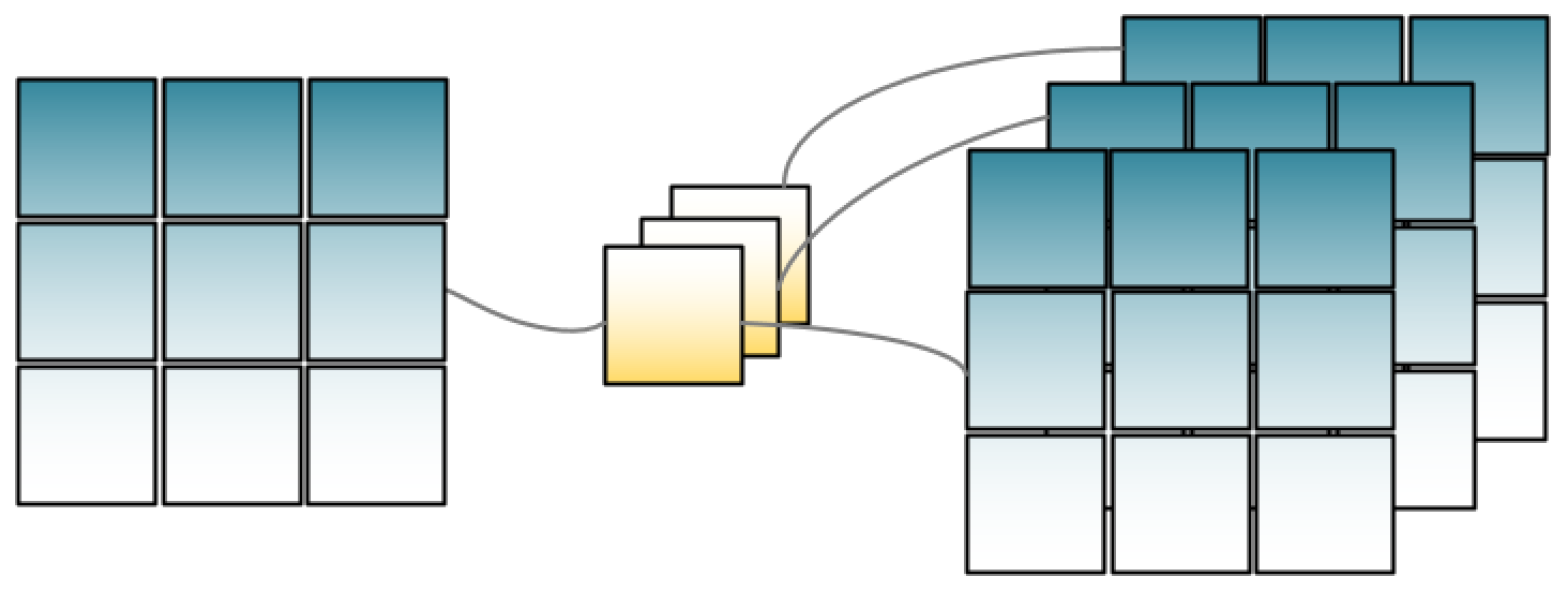
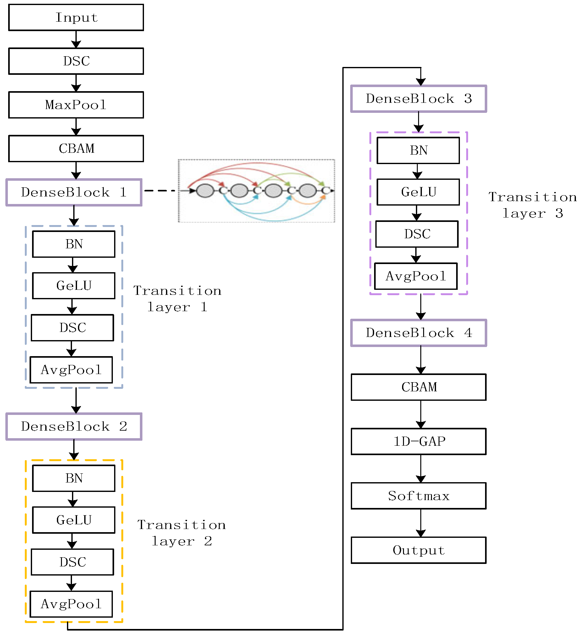
2.1. DenseNet
- It reduces gradient disappearance;
- It enhances feature transmission and more effective utilization of features;
- It reduces parameters and has some inhibition on overfitting.
DenseNet Network Architecture
- (1)
- DenseBlock
- (2)
- Improved composition function
- ①
- Batch normalize
- Calculate the mean of batch processing:
- Calculate the data variance of batch processing:
- Normalize:
- Scale transformation and offset:
- ②
- GeLU active layer
- ③
- A 1 × 3 Convolutional Layer
- (3)
- Transition layer
- ①
- Bottleneck layer
- Increasing/reducing the dimensionality of the channel;
- Adding nonlinear features;
- Realizing the cross-channel information exchange and integration.
- ②
- A 1D average pooling layer
2.2. Improved DenseNet Network Model
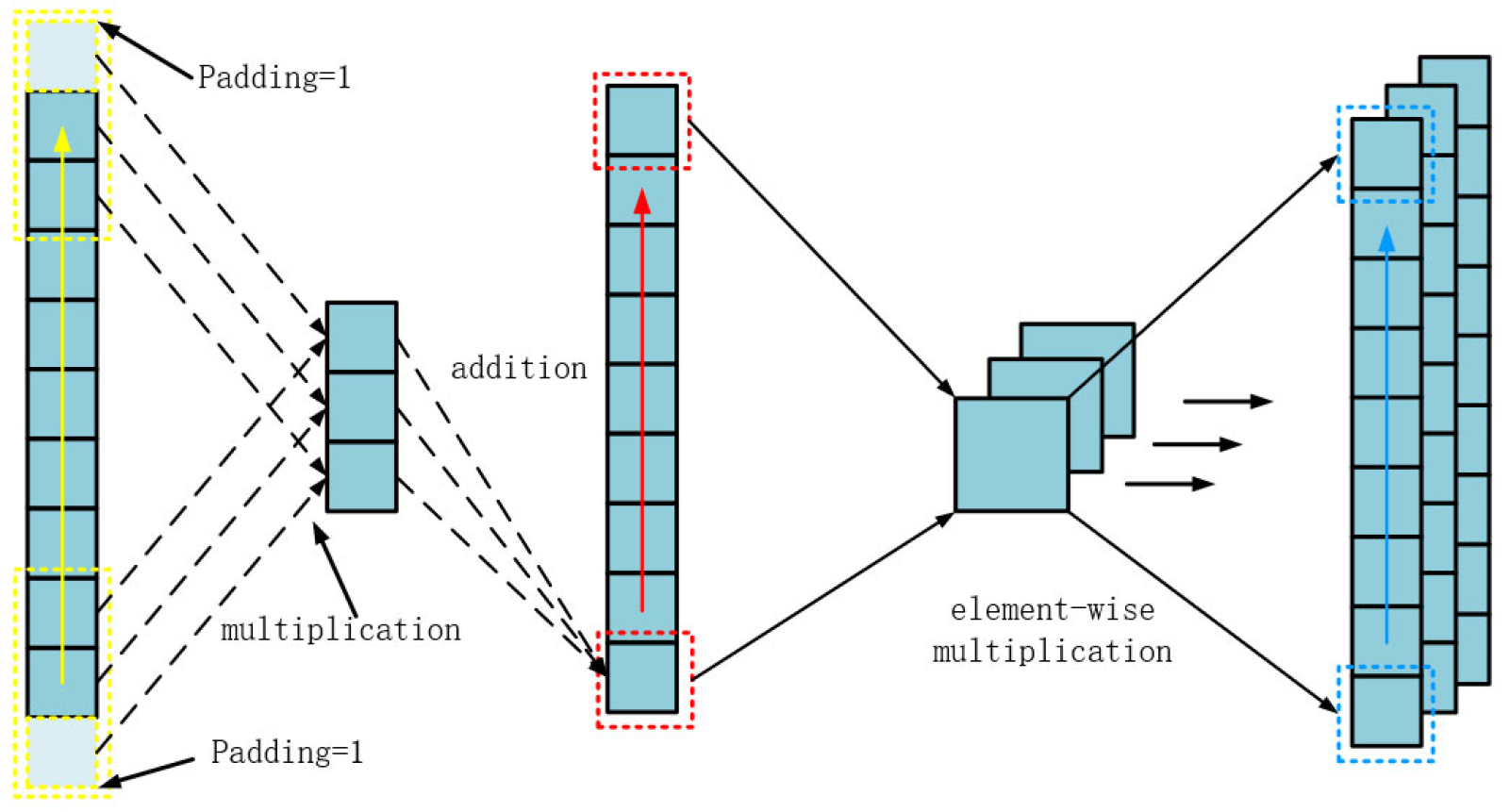
2.2.1. Depthwise Separable Convolution
2.2.2. CBAM Attention Mechanism
2.2.3. 1D Global Average Pooling
- Inhibiting overfitting. Although the FC layer can retain all features, excessive parameters can lead to overfitting. Relatively, GAP has fewer parameters;
- More flexible input size. The feature map parameters processed by GAP are no longer related to the input data size.
2.2.4. Softmax Softmax Classification Layer
3. Experimentation
3.1. Experiment 1: Tennessee Eastman Process Experiment
3.1.1. Introduction to the Experiment
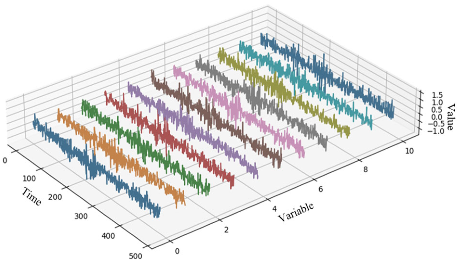
3.1.2. Selection of Experimental Data
3.1.3. The DSCBAM-DenseNet Monitoring Model Established
- Step 1:
- Obtain operating data for 21 operating conditions of the TE process through the MATLAB simulation program;
- Step 2:
- Perform one-hot encoding on all data and tag them with corresponding types;
- Step 3:
- Design the architecture of the DSCBAM DenseNet model and conduct the code implementation;
- Step 4:
- Preprocess the historical data, and first perform normalization processing to eliminate the adverse effects of singular samples; next, random seeds are added to randomly scramble the data and corresponding labels to avoid overfitting of the model; Finally, divide the validation set of the training set by 8:2;
- Step 5:
- Use historical data for model training and validation. If the accuracy of the test set reaches the predetermined standard, proceed to the next step online monitoring. Otherwise, modify the model parameters and retrain the model.
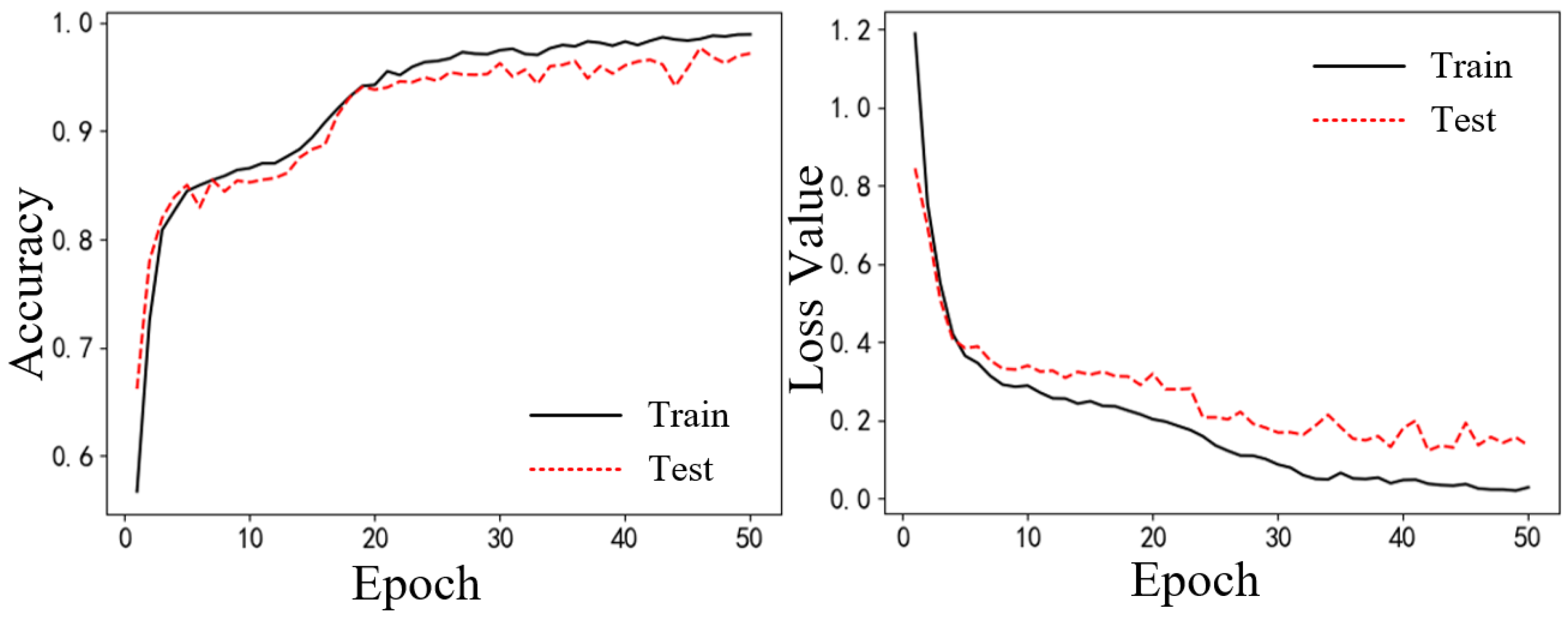
3.1.4. Experimental Results and Comparative Analysis
3.1.5. Supplementary Experiments
3.2. Experiment 2: Compressor Unit Data
3.2.1. Introduction to the Experiment
3.2.2. Experimental Model and Results
4. Conclusions
Author Contributions
Funding
Data Availability Statement
Conflicts of Interest
References
- Xia, M.; Li, T.; Xu, L.; Liu, L.; De Silva, C.W. Fault diagnosis for rotating machinery using multiple sensors and convolutional neural networks. IEEE/ASME Trans. Mechatron. 2017, 23, 101–110. [Google Scholar] [CrossRef]
- Gong, W.; He, L.; Zhang, Z.; Zhou, X.; Cui, S. A novel deep learning method for intelligent fault diagnosis of rotating machinery based on improved CNN-SVM and multichannel data fusion. Sensors 2019, 19, 1693. [Google Scholar] [CrossRef] [PubMed]
- Zhou, D.H.; Liu, Y.; He, X. Review on fault diagnosis techniques for closed-loop systems. Acta Autom. Sin. 2013, 39, 1933–1943. [Google Scholar] [CrossRef]
- Lei, Y.; Yang, B.; Jiang, X.; Jia, F.; Li, N.; Nandi, A.K. Applications of machine learning to machine fault diagnosis: A review and roadmap. Mech. Syst. Signal Process. 2020, 138, 106587. [Google Scholar] [CrossRef]
- Rad, M.A.A.; Yazdanpanah, M.J. Designing supervised local neural network classifiers based on EM clustering for fault diagnosis of Tennessee Eastman process. Chemom. Intell. Lab. Syst. 2015, 146, 149–157. [Google Scholar]
- Wise, B.M.; Gallagher, N.B.; Butler, S.W.; White, D.D.; Barna, G.G. Principal components analysis for monitoring the west valley liquid fed ceramic melter. Waste Manag. 1988, 88, 811–818. [Google Scholar]
- Ge, Z.; Yang, C.; Song, Z. Improved kernel PCA-based monitoring approach for nonlinear processes. Chem. Eng. Sci. 2009, 64, 2245–2255. [Google Scholar] [CrossRef]
- Kano, M.; Hasebe, S.; Hashimoto, I.; Ohno, H.; Egawa, Y.; Shigemoto, T.; Hirochi, T. Monitoring independent components for fault detection. AIChE J. 2003, 49, 969–976. [Google Scholar] [CrossRef]
- Ge, Z.; Song, Z.; Gao, F.; Song, Z. Local ICA for multivariate statistical fault diagnosis in systems with unknown signal and error distributions. AIChE J. 2012, 58, 2357–2372. [Google Scholar] [CrossRef]
- Kresta, J.V.; Macgregor, J.F.; Marlin, T.E. Multivariate statistical monitoring of process operating performance. Can. J. Chem. Eng. 1991, 69, 35–47. [Google Scholar] [CrossRef]
- Wen, Q.; Ge, Z.; Song, Z. Nonlinear dynamic process monitoring based on kernel partial least squares. In Proceedings of the 2012 American Control Conference (ACC), Montreal, QC, Canada, 27–29 June 2012; pp. 2117–2122. [Google Scholar]
- Feng, S.; Cui, J.; Zhang, Z. Fault diagnosis method for an aerospace generator rotating rectifier based on dynamic FFT technology. Metrol. Meas. Syst. 2021, 28, 269–288. [Google Scholar] [CrossRef]
- Tutivén, C.; Figueres, E.; Trilla, L.; Ferrada, P.; Pozo, F. Early fault diagnosis strategy for WT main bearings based on SCADA data and one-class SVM. Energies 2022, 15, 4381. [Google Scholar] [CrossRef]
- Sun, X.; Yu, L.; Zhou, Y.; Li, Y.; Peng, X.; Ma, H.; Wang, H. Research on Fault Diagnosis Method of Distributed Power Distribution Network Based on HHT and CNN. In Proceedings of the 2021 33rd Chinese Control and Decision Conference (CCDC), Kunming, China, 22–24 May 2021; pp. 3682–3687. [Google Scholar]
- Han, H.; Jia, Q.; He, Q.; Li, Z.; Zhao, H. Novel chiller fault diagnosis using deep neural network (DNN) with simulated annealing (SA). Int. J. Refrig. 2021, 121, 269–278. [Google Scholar] [CrossRef]
- Li, S.; Shi, X.; Yang, X.; Ding, X.; Li, Y.; Zhang, W. A review on the signal processing methods of rotating machinery fault diagnosis. In Proceedings of the 2019 IEEE 8th Joint International Information Technology and Artificial Intelligence Conference (ITAIC), Chongqing, China, 24–26 May 2019; pp. 194–198. [Google Scholar]
- Yasenjiang, J.; Zhao, Y.; Liu, Z.; Sun, H.; Liu, Y.; Han, Z. Fault Diagnosis and Prediction of Continuous Industrial Processes Based on Hidden Markov Model-Bayesian Network Hybrid Model. Int. J. Chem. Eng. 2022, 2022, 1–15. [Google Scholar] [CrossRef]
- Chen, J.X.; Shi, H.B. SVM-based Fault Diagnosis for Chemical Process. J. East China Univ. Sci. Technol. (Nat. Sci. Ed.) 2004, 30, 315–317. [Google Scholar]
- Yu, Y.; Cheng, J. A roller bearing fault diagnosis method based on EMD energy entropy and ANN. J. Sound Vib. 2006, 294, 269–277. [Google Scholar] [CrossRef]
- LeCun, Y.; Bengio, Y.; Hinton, G. Deep learning. Nature 2015, 521, 436–444. [Google Scholar] [CrossRef] [PubMed]
- Xie, D.; Bai, L. A hierarchical deep neural network for fault diagnosis on Tennessee-Eastman process. In Proceedings of the 2015 IEEE 14th International Conference on Machine Learning and Applications (ICMLA), Miami, FL, USA, 9–11 December 2015; pp. 745–748. [Google Scholar]
- He, K.; Zhang, X.; Ren, S.; Sun, J. Deep residual learning for image recognition. In Proceedings of the 2016 IEEE Conference on Computer Vision and Pattern Recognition (CVPR), Las Vegas, NV, USA, 27–30 June 2016; pp. 770–778. [Google Scholar]
- Huang, G.; Liu, Z.; Van Der Maaten, L.; Weinberger, K.Q. Densely connected convolutional networks. In Proceedings of the 2017 IEEE Conference on Computer Vision and Pattern Recognition (CVPR), Honolulu, HI, USA, 21–26 July 2017; pp. 2261–2269. [Google Scholar]
- Shi, F.; Wang, Z.; Liang, J. Industrial Fault Identification Based on Semi-supervised Dense Ladder Network. Chem. Eng. J. 2018, 69, 3083–3091. [Google Scholar]
- Li, Y. A fault prediction and cause identification approach in complex industrial processes based on deep learning. Comput. Intell. Neurosci. 2021, 2021, 6612342. [Google Scholar] [CrossRef]
- Yuan, Z.; Yang, Z.; Ling, Y.; Wu, C.; Li, C. Spatiotemporal attention mechanism-based deep network for critical parameters prediction in chemical process. Process Saf. Environ. Prot. 2021, 155, 401–414. [Google Scholar] [CrossRef]
- Mnih, V.; Heess, N.; Graves, A. Recurrent models of visual attention. In Proceedings of the Advances in Neural Information Processing Systems 27 (NIPS 2014), Montreal, QC, Canada, 8–13 December 2014. [Google Scholar]
- Ioffe, S.; Szegedy, C. Batch normalization: Accelerating deep network training by reducing internal covariate shift. In Proceedings of the International Conference on Machine Learning, Lille, France, 7–9 July 2015; pp. 448–456. [Google Scholar]
- Lee, M. GELU Activation Function in Deep Learning: A Comprehensive Mathematical Analysis and Performance. arXiv 2023, arXiv:2305.12073. [Google Scholar]
- Glorot, X.; Bordes, A.; Bengio, Y. Deep sparse rectifier neural networks. In Proceedings of the Fourteenth International Conference on Artificial Intelligence and Statistics, Ft. Lauderdale, FL, USA, 11–13 April 2011; pp. 315–323. [Google Scholar]
- Lin, M.; Chen, Q.; Yan, S. Network in network. arXiv 2013, arXiv:1312.4400. [Google Scholar]
- Goodfellow, I.; Bengio, Y.; Courville, A. Deep Learning; MIT Press: Cambridge, MA, USA, 2016; pp. 1–775. [Google Scholar]
- Sifre, L.; Mallat, S. Rigid-motion scattering for texture classification. arXiv 2014, arXiv:1403.1687. [Google Scholar]
- Zhou, B.; Khosla, A.; Lapedriza, A.; Oliva, A.; Torralba, A. Learning deep features for discriminative localization. In Proceedings of the IEEE Conference on Computer Vision and Pattern Recognition, Las Vegas, NV, USA, 27–30 June 2016; pp. 2921–2929. [Google Scholar]
- Dai, H.; Bai, X.; Chen, J.; Du, Z.; Wang, L.; Zheng, X. SAMAug: Point Prompt Augmentation for Segment Anything Model. arXiv 2023, arXiv:2307.01187. [Google Scholar]
- Downs, J.J.; Vogel, E.F. A plant-wide industrial process control problem. Comput. Chem. Eng. 1993, 17, 245–255. [Google Scholar] [CrossRef]


| No. | Fault Description | Type |
|---|---|---|
| 1 | AC feed ratio, B component remains unchanged | Step |
| 2 | Component B, N/C feed ratio remains unchanged | Step |
| 3 | Feed temperature of D | Step |
| 4 | Inlet temperature of reactor cooling water | Step |
| 5 | Inlet temperature of condenser cooling water | Step |
| 6 | A feed loss | Step |
| 7 | C has pressure loss-reduced availability | Step |
| 8 | A. B, C Feed Composition | Random |
| 9 | Feed temperature of D | Random |
| 10 | Feed temperature of C | Random |
| 11 | Inlet temperature of reactor cooling water | Random |
| 12 | Inlet temperature of condenser cooling water | Random |
| 13 | Reaction dynamics | Slow Drift |
| 14 | Reactor cooling water valve | Stick |
| 15 | Condenser cooling water valve | Stick |
| 16~20 | Unknown | Unknown |
| Variable | Description | Variable | Description |
|---|---|---|---|
| XMEAS(1) | A Feed | XMEAS(14) | Low flow rate at the bottom of the product separator tower |
| XMEAS(2) | D Feed | XMEAS(15) | Stripper level |
| XMEAS(3) | E Feed | XMEAS(16) | Stripper pressure |
| XMEAS(4) | Total feed volume | XMEAS(17) | Stripper tower bottom flow rate |
| XMEAS(5) | Recirculation flow rate | XMEAS(18) | Stripper temperature |
| XMEAS(6) | Discharge valve | XMEAS(19) | Stripper flow rate |
| XMEAS(7) | Reactor level | XMEAS(20) | Compressor power |
| XMEAS(8) | Reactor temperature | XMEAS(21) | Reactor cooling water outlet temperature |
| XMEAS(9) | Discharge speed | XMEAS(22) | Outlet temperature of separator cooling water |
| XMEAS(10) | Product separator temperature | XMEAS(23~28) | Component A~F |
| XMEAS(11) | Product separator liquid level | XMEAS(29~36) | Component A~H |
| XMEAS(12) | Reactor level | XMEAS(37~41) | Component A~H |
| XMEAS(13) | Product separator pressure |
| Variable | Description | Variable | Description |
|---|---|---|---|
| XMV(1) | D Feed | XMV(7) | Liquid flow rate of separator tank |
| XMV(2) | E Feed | XMV(8) | Stripper liquid product flow rate |
| XMV(3) | A Feed | XMV(9) | Stripper water flow valve |
| XMV(4) | Total feed volume | XMV(10) | Reactor cooling water flow rate |
| XMV(5) | Compressor Recirculation Valve | XMV(11) | Cooling water flow rate of condenser |
| XMV(6) | Discharge valve | XMV(12) | Stirring speed |
| Layers | Network Parameters | Output Shape |
|---|---|---|
| Conv | 1 × 7 conv, stride 2, padding 3 | [−1, 64, 112] |
| MaxPool | 1 × 3 max pool, stride 2, padding 1 | [−1, 64, 56] |
| DenseBlock1 | [−1, 256, 56] | |
| Transition Layer1 | 1 × 1 conv | [−1, 128, 56] |
| 1 × 2 average pool, stride 2 | [−1, 128, 28] | |
| DenseBlock2 | [−1, 512, 28] | |
| Transition Layer2 | 1 × 1 conv | [−1, 256, 28] |
| 1 × 2 average pool, stride 2 | [−1, 256, 14] | |
| DenseBlock3 | [−1, 1024, 14] | |
| Transition Layer3 | 1 × 1 conv | [−1, 512, 14] |
| 1 × 2 average pool, stride 2 | [−1, 512, 7] |
| Results | 1 | 2 | 3 | 4 | 5 | 6 | 7 | 8 | 9 | 10 | Acc & Std |
|---|---|---|---|---|---|---|---|---|---|---|---|
| Normal | 98.15 | 98.34 | 98.69 | 98.4 | 98.76 | 98.3 | 98.38 | 97.57 | 98.51 | 98.38 | 98.35 ± 0.33 |
| Fault 1 | 100 | 100 | 99.85 | 99.9 | 99.9 | 99.85 | 100 | 99.8 | 100 | 99.75 | 99.91 ± 0.09 |
| Fault 2 | 100 | 100 | 99.83 | 99.41 | 99.77 | 100 | 100 | 99.77 | 99.49 | 100 | 99.83 ± 0.22 |
| Fault 3 | 90.17 | 91.25 | 92.2 | 90.89 | 90.71 | 92.1 | 93 | 90.95 | 91.01 | 92.16 | 91.44 ± 0.87 |
| Fault 4 | 98.48 | 97.97 | 97.5 | 96.77 | 97.85 | 97.97 | 96.96 | 96.39 | 97.47 | 95.57 | 97.29 ± 0.87 |
| Fault 5 | 93.51 | 91.81 | 92.86 | 91.35 | 93.05 | 93.12 | 92.6 | 91.35 | 90.37 | 92.66 | 92.27 ± 1 |
| Fault 6 | 100 | 99.78 | 100 | 99.78 | 100 | 100 | 100 | 100 | 100 | 100 | 99.96 ± 0.09 |
| Fault 7 | 99.35 | 99.51 | 100 | 100 | 99.67 | 99.35 | 99.59 | 100 | 100 | 100 | 99.75 ± 0.52 |
| Fault 8 | 98.15 | 97.99 | 98.57 | 97.65 | 97.32 | 97.9 | 98.15 | 97.65 | 97.23 | 96.81 | 97.74 ± 0.52 |
| Fault 9 | 87.72 | 84.69 | 88.1 | 84.5 | 86.89 | 85.98 | 88.27 | 85.88 | 89.37 | 86.98 | 86.84 ± 1.58 |
| Fault 10 | 91.81 | 88.61 | 89.31 | 92.01 | 91.71 | 91.97 | 91.61 | 91.71 | 90.31 | 92.61 | 91.17 ± 1.31 |
| Fault 11 | 87.33 | 85.67 | 88.68 | 88.99 | 86.81 | 89.1 | 88.89 | 88.16 | 88.68 | 87.44 | 87.98 ± 1.13 |
| Fault 12 | 97.11 | 96.3 | 96.4 | 97.34 | 94.44 | 96.88 | 96.76 | 95.95 | 95.72 | 96.53 | 96.34 ± 0.83 |
| Fault 13 | 98 | 97.12 | 97.5 | 98.37 | 98 | 98.62 | 98.12 | 98.25 | 97.25 | 97.5 | 97.87 ± 0.5 |
| Fault 14 | 96.29 | 93.72 | 95.72 | 95.86 | 96.15 | 96.58 | 95.86 | 96.72 | 96.86 | 95.86 | 95.96 ± 0.88 |
| Fault 15 | 84.36 | 81.15 | 83.3 | 84.22 | 83.66 | 86.03 | 84.78 | 83.94 | 80.87 | 84.92 | 83.72 ± 1.62 |
| Fault 16 | 82.23 | 82.7 | 83.1 | 81.92 | 81.45 | 84.12 | 85.69 | 77.2 | 80.35 | 82.55 | 82.13 ± 2.26 |
| Fault 17 | 94.52 | 95.21 | 96.23 | 94.96 | 94.52 | 94.18 | 95.38 | 94.52 | 92.81 | 96.06 | 94.84 ± 0.98 |
| Fault 18 | 97.43 | 96.06 | 97.09 | 97.09 | 96.4 | 98.63 | 96.23 | 96.06 | 95.21 | 96.75 | 96.70 ± 0.94 |
| Fault 19 | 87.09 | 82.49 | 87.31 | 86.43 | 86.87 | 86.65 | 89.72 | 87.31 | 84.46 | 87.96 | 86.63 ± 1.96 |
| Fault 20 | 90.31 | 89.92 | 90.89 | 90.7 | 87.4 | 92.05 | 88.76 | 90.7 | 87.98 | 90.5 | 89.92 ± 1.44 |
| Mean | 93.91 | 92.87 | 93.96 | 93.64 | 93.40 | 94.26 | 94.23 | 93.33 | 93.05 | 93.86 | 93.65 ± 0.48 |
| Fault Type | DSCBAM-DenseNet | DenseNet | ResNet | KNN | MLP | NB | SVM |
|---|---|---|---|---|---|---|---|
| Normal | 98.35 | 98.24 | 82.98 | - * | - | - | - |
| Fault 1 | 100 | 98.2 | 100 | 99.25 | 95.25 | 95.63 | 98.5 |
| Fault 2 | 100 | 100 | 100 | 96.88 | 97.13 | 98 | 96.75 |
| Fault 3 | 91.44 | 90 | 71.43 | 58.38 | 30 | 55.88 | 86.25 |
| Fault 4 | 97.29 | 96.96 | 97.87 | 98.75 | 96.63 | 100 | 100 |
| Fault 5 | 92.27 | 90.43 | 91.35 | 58.63 | 41.13 | 42.88 | 29.63 |
| Fault 6 | 100 | 100 | 96.38 | 100 | 96.38 | 99.75 | 99.5 |
| Fault 7 | 100 | 100 | 94.5 | 99.75 | 94.5 | 100 | 99.5 |
| Fault 8 | 97.74 | 96.9 | 97.65 | 77.13 | 55.75 | 96.5 | 40.75 |
| Fault 9 | 86.84 | 86.17 | 70.45 | 53 | 37.5 | 43.5 | 56.5 |
| Fault 10 | 91.17 | 89.97 | 92.5 | 63.5 | 47.88 | 80.25 | 23.88 |
| Fault 11 | 87.98 | 83.21 | 91.11 | 74.25 | 66.63 | 94 | 23 |
| Fault 12 | 96.34 | 92.64 | 87 | 75.13 | 43.75 | 93.25 | 21.13 |
| Fault 13 | 97.87 | 95.2 | 88 | 87.25 | 72.88 | 93.75 | 27.88 |
| Fault 14 | 95.96 | 97.64 | 92 | 99.875 | 50.5 | 100 | 92 |
| Fault 15 | 83.72 | 80.45 | 67.39 | 55.13 | 60.25 | 40.13 | 53.25 |
| Fault 16 | 82.13 | 62.4 | 78.38 | 68.38 | 68.25 | 55.38 | 53.88 |
| Fault 17 | 94.84 | 91.3 | 89 | 99.5 | 92.5 | 100 | 97.25 |
| Fault 18 | 96.70 | 87.01 | 97.5 | 87.25 | 80.75 | 88.5 | 74.5 |
| Fault 19 | 86.63 | 85.18 | 77.5 | 77.25 | 46.63 | 77.38 | 37 |
| Fault 20 | 89.92 | 88.71 | 90 | 69.25 | 65.63 | 75.38 | 69.75 |
| Mean | 93.62 | 90.62 | 88.5 | 79.93 | 66.99 | 81.51 | 64.04 |
| SNR | −5 | −1 | 0 | 1 | 5 |
|---|---|---|---|---|---|
| 21-Acc | 87.41 | 88.15 | 87.48 | 91.70 | 91.79 |
| Std | 0.37 | 0.7 | 0.52 | 0.83 | 0.21 |
| Classes | Type | Precision | Recall | F1 Score |
|---|---|---|---|---|
| Normal | Step | 0.85 | 0.98 | 0.87 |
| Fault 1 | Step | 0.88 | 0.93 | 0.91 |
| Fault 2 | Step | 0.89 | 0.95 | 0.92 |
| Fault 3 | Step | 0.82 | 0.90 | 0.86 |
| Fault 4 | Step | 0.84 | 0.92 | 0.88 |
| Fault 5 | Step | 0.87 | 0.93 | 0.89 |
| Fault 6 | Step | 0.90 | 0.95 | 0.92 |
| Fault 7 | Random | 0.87 | 0.88 | 0.88 |
| Fault 8 | Random | 0.87 | 0.88 | 0.86 |
| Fault 9 | Random | 0.88 | 0.87 | 0.88 |
| Fault 10 | Random | 0.85 | 0.88 | 0.86 |
| Fault 11 | Random | 0.88 | 0.82 | 0.85 |
| Fault 12 | Slow Drift | 0.89 | 0.87 | 0.88 |
| Fault 13 | Stick | 0.89 | 0.85 | 0.87 |
| Fault 14 | Stick | 0.86 | 0.82 | 0.84 |
| Fault 15 | Unknown | 0.77 | 0.68 | 0.73 |
| Fault 16 | Unknown | 0.87 | 0.86 | 0.86 |
| Fault 17 | Unknown | 0.91 | 0.87 | 0.89 |
| Fault 18 | Unknown | 0.96 | 0.84 | 0.89 |
| Fault 19 | Unknown | 0.92 | 0.82 | 0.86 |
| Fault 20 | Unknown | 0.93 | 0.84 | 0.88 |
| Results | 1 | 2 | 3 | 4 | 5 | 6 | 7 | 8 | 9 | 10 | Acc & Std |
|---|---|---|---|---|---|---|---|---|---|---|---|
| Normal | 100 | 100 | 99.72 | 100 | 100 | 99.64 | 99.8 | 100 | 100 | 100 | 99.91 ± 0.14 |
| ShutDown | 98.22 | 96.72 | 97.36 | 98.77 | 98.43 | 98.22 | 98.49 | 97.98 | 98.4 | 97.61 | 98.07 ± 0.62 |
| Mean | 99.11 | 98.36 | 98.54 | 99.39 | 99.22 | 98.93 | 99.15 | 98.99 | 99.20 | 98.81 | 98.99 ± 0.32 |
Disclaimer/Publisher’s Note: The statements, opinions and data contained in all publications are solely those of the individual author(s) and contributor(s) and not of MDPI and/or the editor(s). MDPI and/or the editor(s) disclaim responsibility for any injury to people or property resulting from any ideas, methods, instructions or products referred to in the content. |
© 2024 by the authors. Licensee MDPI, Basel, Switzerland. This article is an open access article distributed under the terms and conditions of the Creative Commons Attribution (CC BY) license (https://creativecommons.org/licenses/by/4.0/).
Share and Cite
Yasenjiang, J.; Lan, Z.; Wang, K.; Lv, L.; He, C.; Zhao, Y.; Wang, W.; Gao, T. Fault Monitoring Method for the Process Industry System Based on the Improved Dense Connection Network. Mathematics 2024, 12, 2843. https://doi.org/10.3390/math12182843
Yasenjiang J, Lan Z, Wang K, Lv L, He C, Zhao Y, Wang W, Gao T. Fault Monitoring Method for the Process Industry System Based on the Improved Dense Connection Network. Mathematics. 2024; 12(18):2843. https://doi.org/10.3390/math12182843
Chicago/Turabian StyleYasenjiang, Jiarula, Zhigang Lan, Kai Wang, Luhui Lv, Chao He, Yingjun Zhao, Wenhao Wang, and Tian Gao. 2024. "Fault Monitoring Method for the Process Industry System Based on the Improved Dense Connection Network" Mathematics 12, no. 18: 2843. https://doi.org/10.3390/math12182843
APA StyleYasenjiang, J., Lan, Z., Wang, K., Lv, L., He, C., Zhao, Y., Wang, W., & Gao, T. (2024). Fault Monitoring Method for the Process Industry System Based on the Improved Dense Connection Network. Mathematics, 12(18), 2843. https://doi.org/10.3390/math12182843