Deep Learning-Enhanced Autoencoder for Multi-Carrier Wireless Systems

Abstract

In a multi-carrier (MC) system, the transmitted data are split across several sub-carriers as a crucial approach for achieving high data rates, reliability, and spectral efficiency. Deep learning (DL) enhances MC systems by improving signal representation, leading to more efficient data transmission and reduced bit error rates. In this paper, we propose an MC system supported by DL for operation on fading channels. Deep neural networks are utilized to model the modulation block, while a gated recurrent unit (GRU) network is used to model the demodulation blocks, acting as the encoder and decoder within an autoencoder (AE) architecture. The proposed scheme, known as MC-AE, differs from existing AE-based systems by directly processing channel state information and the received signal in a fully data-driven way, unlike traditional methods that rely on channel equalizers. This approach enables MC-AE to improve diversity and coding gains in fading channels by simultaneously optimizing the encoder and decoder. In this experiment, we evaluated the performance of the proposed model under both perfect and imperfect channel conditions and compared it with other models. Additionally, we assessed the performance of the MC-AE system against index modulation-based MC systems. The results demonstrate that the GRU-based MC-AE system outperforms the others.

1. Introduction

Multicarrier (MC) transmission [1] has been recognized and adopted by numerous standards bodies for both wireline and wireless systems [2,3] due to its effectiveness and reliability. This approach offers several benefits, including resistance to single-frequency interference and enhanced capability to reduce inter-symbol interference (ISI). MC’s strength in addressing various channel impairments, such as frequency selectivity and impulse noise, makes it a popular choice in emerging applications like wireless local area networks (WLANs) [4] and power line communications (PLCs) [5].

The core concept of the MC protocol is the decomposition of the spectrum into a series of orthogonal narrowband subchannels, using complex exponentials as carriers of information [6]. Two primary MC techniques are commonly employed: discrete multitone (DMT) [7] for wireline systems and orthogonal frequency-division multiplexing (OFDM) [8], which is predominantly used in wireless applications. Both OFDM and DMT rely on fast Fourier transform (FFT) for spectrum decomposition, and data are transmitted in blocks as a result. Many wireless standards, such as IEEE 802.11, IEEE 802.16, 3GPP LTE, and LTE-Advanced, utilize an OFDM-based multicarrier system [9].

A variety of sophisticated MC methods built on OFDM have been investigated recently with the goal of improving spectral or energy efficiency. For example, spread OFDM (S-OFDM), using a Walsh–Hadamard spreading matrix, was proposed in [10], where each subcarrier in the OFDM system is modulated using a spread spectrum technique. In [11], the author introduced OFDM with index modulation (OFDM-IM), employing a maximum likelihood (ML) detector to identify the received signal. Compared to traditional OFDM, OFDM-IM offers enhanced reliability and energy efficiency by activating only a subset of subcarriers. This method transmits data bits through active indices in addition to M-ary symbols. The study in [12] revealed that, like conventional OFDM, OFDM-IM has a diversity order of one and examined its error performance. In particular, spread OFDM-IM (S-OFDM-IM) was developed in [13] by applying a spreading code to OFDM-IM to enhance its diversity advantage. This experiment demonstrates that when low-complexity detection techniques, like minimum mean squared error (MMSE)-based detectors, are used, S-OFDM-IM performs better than S-OFDM. Similarly, the dual model OFDM (DM-OFDM) was introduced in [14] and used several distinct signal constellations.

Recently, deep learning (DL) has been applied to various areas within the communications field, particularly to address physical layer challenges [15,16]. DL has also been widely utilized to tackle issues in MC systems [17]. For instance, deep neural networks (DNNs) have been effectively employed to detect OFDM and OFDM-IM signals [18,19], particularly in the presence of channel impairments. In [20], a convolutional neural network (CNN)-based receiver was designed for joint detection and modulation classification of the received signal. The work in [21] introduced a dual CNN-based decoder for channel estimation in a multiple input multiple output OFDM (MIMO-OFDM) system, aiming to reduce complexity by incorporating an additional neural network, referred to as HyperNet. A long short-term memory (LSTM)-based detector for the OFDM-IM system was proposed in [22]. A Y-shaped net-based bi-diretional LSTM (Bi-LSTM) model was proposed for the OFDM-IM system in [23].

The concept of an end-to-end communication system modeled as an autoencoder (AE) in DNNs was first introduced in [24]. In this approach, the transmitter encodes the input data so that the receiver’s output is optimized to match the original input. Additionally, ref. [25] demonstrated the ease of implementing these techniques using open-source DNN frameworks and commercially available software-defined radios. Building on these ideas, ref. [26] proposed an AE-based end-to-end communication system capable of handling unknown channel models. In [27], the authors proposed a novel deep energy EA for noncoherent multicarrier multiuser SIMO (MU-SIMO) systems in fading channels. The EA-based approach, using neural networks for both transmitter and receiver, leverages energy-only input at the decoder and optimizes subcarrier power levels. In [28], the authors proposed a novel peak-to-average power ratio (PAPR) reduction scheme, PRNet, for OFDM systems based on deep AE architecture. The scheme adaptively determines constellation mapping and demapping using DL, minimizing both bit error rate (BER) and PAPR. For fading channels, ref. [29] introduced a radio transformer network (RTN) to counteract fading, but it did not leverage multipath diversity. Similarly, the AE method applying individual OFDM sub-carriers in [29] did not provide diversity advantages. The paper in [30] compared an AE-based OFDM system with IEEE 802.11a Wi-Fi, demonstrating that the AE system adapts better to channel conditions and effectively manages multi-path effects. A CNN-based universal filtered MC system was proposed in [31], where the DL models leverage the typically discarded odd-indexed samples from the received signal. Consequently, the model relies heavily on extensive and diverse training data to perform effectively. A DNN-based MC with AE (MC-AE) for fading channels was proposed in [32], where both modulation and demodulation are handled by neural networks without relying on channel equalizers. The approach improves diversity and coding gains, achieving superior BLER performance over traditional methods, and is extended to MU-MC-AE. Another DNN-based turbo-style MC-AE was proposed in [33] for the OFDM system, incorporating the exchange of extrinsic information between the MC-AE decoder and the soft-decision channel decoder, which adds computational complexity. The gated recurrent unit (GRU) model captures long-term dependencies in sequential data through gating mechanisms, effectively addressing the vanishing gradient problem. GRUs have a simpler structure with fewer parameters than LSTMs, enabling faster training efficiency. Additionally, GRUs require less memory than LSTMs and generalize well with smaller datasets, making them suitable for real-time and resource-constrained applications [34,35]. Meanwhile, AEs are advantageous for feature extraction and dimensionality reduction, allowing data compression and efficient representation learning, which often enhances performance in downstream tasks [36]. In this paper, we propose a GRU-based MC-AE (GRU-MC-AE) system that leverages the advantages of the GRU model to tackle the previously mentioned challenges. In this paper, we evaluate the BER and block error rate (BLER) performance of the proposed model across various signal-to-noise ratios (SNRs) under both perfect and imperfect channel conditions. Additionally, we calculate the spectral efficiency (SE) and energy efficiency (EE) across various SNR levels. We compare its performance with traditional decoders and other DL-based decoders. The simulation results demonstrate that our proposed GRU-MC-AE model outperforms both conventional and DL-based models. The key contributions of this paper are summarized below:

• This study proposes a single-user MC-AE system, wherein a DNN model is used for the modulation block and the demodulation block is implemented using a GRU, acting as the encoder and decoder in an AE framework. The encoder employs a linear activation function, which passes the weighted sum of inputs directly to produce continuous outputs and the GRU-based decoder effectively manages the temporal dependencies between subcarriers, enhancing the system’s ability to adapt to changing channel conditions.
• The suggested method does not require an equalization or domain knowledge because it feeds the decoder both the received signal and the channel state information (CSI) directly. The encoder and decoder are efficiently learned by this totally data-driven method to maximize diversity and coding gains in fading channels.
• We evaluate the performance of the proposed model in terms of BER and BLER under both perfect and imperfect channel conditions. We compare it with traditional and DL-based decoders, and the results show that the GRU-MC-AE model exceeds the performance of both conventional and DL-based models. To further assess the efficiency of the proposed model, we evaluate its SE and EE.

The remainder of this paper is organized as follows: The system modeling is introduced in Section 2. A thorough discussion of the suggested model, including details on offline training and online testing protocols, is given in Section 3. The simulation results are presented in Section 4, while the complexity analysis and detailed discussion are provided in Section 5 and Section 6, respectively. Finally, the conclusions are drawn in Section 7.

2. System Model

In an MC-AE system, the incoming message is passed through the modulation section, which consists of a DL-based encoder, generating a transmitted data vector. This data vector is then processed through a time-domain OFDM (t-OFDM) operation. Specifically, an inverse fast Fourier transform (IFFT) is applied to convert the data into the time domain, and a cyclic prefix is added to combat inter-symbol interference before the signal is transmitted through a fading channel with noise. At the receiver, the cyclic prefix is removed, and an inverse time-domain OFDM operation is performed using a fast Fourier transform (FFT) to convert the signal back into the frequency domain. The M-ary QAM/PSK modulation or several newly developed instant messaging systems [37] are examples of modulation schemes. The resulting received signal is then passed through a demodulation block, which consists of a DL-based decoder that generates the estimated output.

The general structure of the proposed MC-AE system is shown in Figure 1. In our proposed system, the incoming message s is fed as input to the encoder. In the MC-AE encoder, each incoming message $sϵS=\{s_1,\dots ,s_M\}$, where $M=2^m$ and consists of a bit-stream of m bits, is mapped into a one-hot vector s of size $M\times 1$. This vector has all zero entries except for a single one. Afterward, the DL-based encoder produces the transmitted data vector $\overline{\mathbf{x}}={[x_1,x_2,\cdots ,x_{N_c}]}^T$, where $N_c$ denotes the number of sub-carriers. In a manner similar to the IM-based scheme [38], the proposed MC-AE system splits the total $N_c$ subcarriers into G groups, each containing N subcarriers, such that $N_c=NG$. The AE structure is then applied independently to each group. Following processing by the t-OFDM block, $\mathbf{x}$ is transmitted to the receiver where it is impeded by additive noise $\mathbf{w}$ after first going via the fading channel $\mathbf{H}$. After performing the inverse t-OFDM operation at the receiver, the received signal $\mathbf{y}$ is obtained. The received received frequency domain signal $\mathbf{y}$ is expressed as follows:

$$\mathbf{y}=\mathbf{H}\odot \mathbf{x}+\mathbf{w},$$

(1)

In this equation, w represents the AWGN, where ${\mathbf{w}}_i\sim \mathcal{CN}(0,{\sigma }^2)$. The $\mathbf{H}=\left[H_1,\cdots ,H_N\right]$ denotes the Rayleigh fading channel, where ${\mathcal{H}}_i\sim \mathcal{CN}(0,1)$ and the operator ⊙ signifies element-wise multiplication. It is assumed that the average energy of the transmitted M-ary symbol is $E_a$, resulting in an average SNR at the receiver of $\overline{\gamma }=E_a/{\sigma }^2$.

In order to decode the signal, we assume that the received signal $\mathbf{y}$ and the CSI are both fully known at the receiver and are fed into the decoder as inputs. The real vector $\widehat{\mathbf{x}}={[{\mathbf{y}}_R,{\mathbf{y}}_I,{\mathbf{H}}_R,{\mathbf{H}}_I]}^T$ is specifically created from the complex vectors $\mathbf{y}$ and $\mathbf{H}$ where the real and imaginary components of $\mathbf{y}$ and $\mathbf{H}$ are denoted, respectively, by ${\mathbf{y}}_R,{\mathbf{y}}_I$ and ${\mathbf{H}}_R,{\mathbf{H}}_I$. The proposed MC-AE significantly differs from traditional RTN-based AE schemes [29]. RTN is designed for block fading channels where sub-carrier channels remain constant over multiple uses. This allows RTN to operate without CSI, relying instead on the domain knowledge of a channel equalizer. These properties make it a model-driven, noncoherent approach. On the other hand, the proposed MC-AE is designed for time-varying channel conditions, in which the channel coefficients fluctuate arbitrarily with each usage. This flexibility enables the proposed scheme to utilize perfect CSI at the receiver in a fully data-driven manner to exploit frequency diversity across different sub-carriers, moving away from the reliance on domain knowledge characteristic of RTN.

For the imperfect CSI settings, we consider an actual system that faces difficulties because of the erroneous CSI assessment of the receiver. The imprecise calculation of CSI at the receiver leads to system performance degradation, especially in scenarios where accurate channel estimation is crucial for effective signal detection and decoding. The estimated channel $h\left(\alpha \right)$ is modeled as follows:

$$h\left(\alpha \right)=\widehat{h}\left(\alpha \right)+E\left(\alpha \right),$$

(2)

where $E\left(\alpha \right)\sim \mathcal{CN}(0,{ϵ}^2)$ represents the channel estimation error, and $\widehat{h}\left(\alpha \right)\sim \mathcal{CN}\left(0,{\displaystyle \frac{1}{{ϵ}^2}}\right)$ is the imperfect estimate of the channel. Here, ${ϵ}^2$ denotes the error variance in the CSI estimation. In this model, the channel estimation error variance ${ϵ}^2$ is dependent on the average SNR ($\overline{\gamma }$) and is defined as ${ϵ}^2={\displaystyle \frac{1}{1+\overline{\gamma }}}$. Thus, as the SNR increases, the channel estimation error variance decreases, reflecting improved CSI accuracy at higher SNR values [12].

3. Proposed GRU-MC-AE Network Architecture

The structure of the proposed GRU-MC-AE network is shown in Figure 2. Our proposed model consists of three main parts: a DL-based encoder, a channel, and a DL-based decoder. The encoder section includes an input layer, a dense layer, a normalization layer, and a reshape layer. In the encoder, one of the $M=2^m$ possible incoming messages s is mapped to a one-hot vector $\mathbf{s}$ of size $M\times 1$, where all entries are zero except for one, which is set to one. The next layer is a dense layer with a linear activation function. This layer produces a $2N$-dimensional vector $\mathbf{u}$. The operation of this layer is expressed as follows:

$$\mathbf{u}=\mathbf{W}\mathbf{s}+\mathbf{b},$$

(3)

where $\mathbf{w}$ is the weight and $\mathbf{b}$ is the bias vector. The following layer is a normalization layer implemented as a lambda function, which regulates the average transmission power for each subcarrier. The output of this layer is a $2N$-dimensional vector represented as follows:

$$\mathbf{v}=\sqrt{N{E}_a}\mathbf{u}/\Vert \mathbf{u}\Vert ,$$

(4)

where $E_a$ is the average energy of the transmitted symbol. The next layer is the reshape layer, which generates the real and imaginary parts by reshaping $\mathbf{v}$ into an $N\times 1$ complex-valued vector. The subsequent section is the channel implemented with a lambda layer, where noise is added to the signal. After passing through the channel, the output consists of both the received signal and the estimated channel coefficients.

The final section is the decoder, which consists of an input layer, two GRU layers, and an output layer. In the input layer, a $4N$-dimensional real vector, denoted as $\widehat{\mathbf{x}}$, is constructed from the complex vectors $\mathbf{y}$ and $\mathbf{H}$. This vector is then fed into the GRU layers, which have $Q_1$ and $Q_2$ hidden nodes, respectively. The first GRU layer processes the channel output and generates a hidden state with $Q_1$ units for each subcarrier. 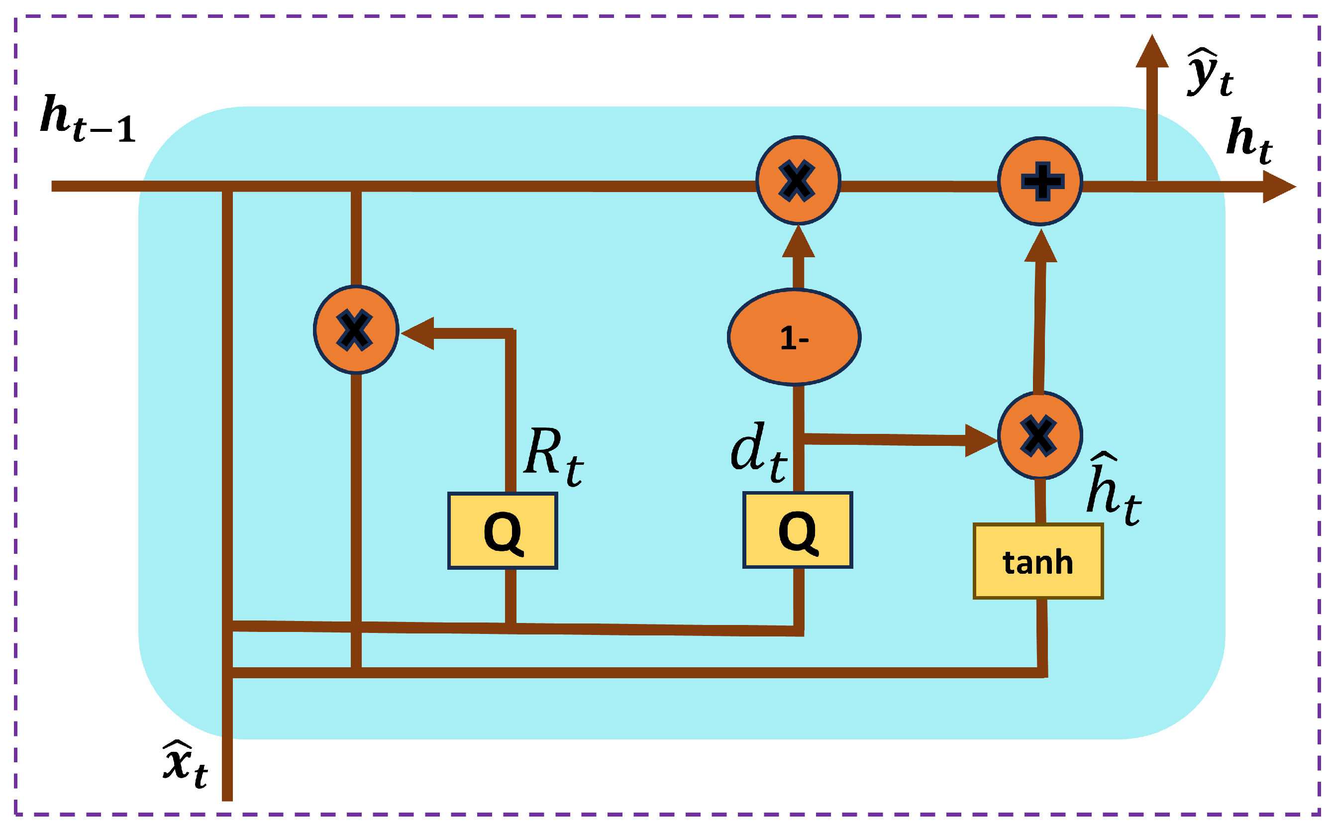The second GRU layer further reduces the sequence to produce a single output vector of $Q_2$ units. The internal structure of the GRU model is illustrated in Figure 3. The GRU streamlines the traditional RNN by incorporating two key gates: the update gate and the reset gate. The update gate manages the portion of the previous hidden state that is passed to the next time step, enabling the model to retain information across longer sequences. Conversely, the reset gate controls how much of the previous hidden state is discarded, allowing the model to clear its memory when it is necessary. The candidate hidden state is calculated using the current input and the reset hidden state, and the final hidden state is determined by combining the previous hidden state with the candidate state, based on the update gate’s influence [39,40].

The update gate, represented as $d_t$, controls the extent to which the previous hidden state $h_{t-1}$ is retained and passed on to the next time step. The reset gate, denoted as $R_t$, regulates how much of the previous hidden state $h_{t-1}$ should be discarded or reset before incorporating the new input. The candidate hidden state, ${\widehat{h}}_t$, represents the newly computed memory content, which is generated based on the current input and the modified hidden state. The final hidden state $h_t$ at time step t is a combination of the previous hidden state $h_{t-1}$ and the candidate hidden state ${\widehat{h}}_t$, controlled by the update gate $d_t$. The operation of the gates and hidden states in the GRU can be expressed as follows:

$$d_t=\sigma (W_d·{\widehat{x}}_t+U_d·h_{t-1}+b_d),$$

(5)

$$R_t=\sigma (W_R·{\widehat{x}}_t+U_R·h_{t-1}+b_R),$$

(6)

$${\widehat{h}}_t=tanh(W_h·{\widehat{x}}_t+U_h·(R_t\odot h_{t-1})+b_h),$$

(7)

$$h_t=(1-d_t)\odot h_{t-1}+d_t\odot {\widehat{h}}_t,$$

(8)

where $\sigma$ represents the sigmoid activation function, $tanh$ denotes the hyperbolic tangent function, ⊙ represents element-wise (Hadamard) multiplication, $b_d$, $b_R$, $b_h$ are the bias vectors, $W_d$, $W_R$, $W_h$ are the weight matrices, and $U_d$, $U_R$, $U_h$ are the recurrent weight matrices for the update, reset, and candidate hidden state, respectively.

The final layer of the decoding section is a dense layer with M nodes, utilizing a softmax activation function. By utilizing the softmax, the decoder produces a probability vector $\widehat{s}={[{\widehat{s}}_1,\cdots ,{\widehat{s}}_M]}^T$, where the i-th entry represents the likelihood that the corresponding message is transmitted. The largest entry of $\widehat{s}$ is used to determine the estimated message $\widehat{s}$. Applying softmax enables the model to produce a clear and interpretable output with values that sum is 1. This allows the output to be evaluated based on the correct predicted symbol, similar to a classification setup in communication systems [41]. If ${\theta }_{\mathrm{dec}}={\{W_i,b_i\}}_{i=1,2}$ denote the parameters and z denotes the input of the output layer, the output is expressed as follows:

$$\widehat{s}={\sigma }_{\mathrm{Softmax}}(Wz+b),$$

(9)

where ${\sigma }_{\mathrm{Softmax}}$ represent the softmax activation functions. The detailed signal detection process for the proposed GRU-based decoder in the MC-AE system is systematically presented in Algorithm 1. This algorithm provides a structured overview of each stage, including data generation, AE model design, training, and testing. The step-by-step organization offers a clear perspective on the entire workflow.

Algorithm 1 MC-AE Model Setup, Training, and Evaluations

1: Initialize Parameters: N, M, m, R (bit rate), SNR, batch size, norm type, epochs, learning rate, hidden layers, loss function, train/test sizes, activation functions   2: Define noise_std based on training SNR   3: Define Channel Layers   4: Function channel(Z):   5:     Initialize channel estimate $H_{\mathrm{est}}$ with noise   6:     Calculate real and imaginary parts with noise added   7:     Return received signal y   8: Function channel_test(Z, noise_std, test_size, imperfect_channel=False):   9: if imperfect_channel then 10:         Calculate imperfect CSI error 11: end if 12:     Add noise to channel estimates 13:     Calculate received signal y 14:     Return y 15: Build MC-AE Model 16: Create input layer for encoder 17: Add dense encoding layer 18: Normalize encoder output based on norm type 19: Reshape encoder output 20: Define decoder GRU layers and Dense output layer 21: Construct complete Autoencoder model 22: Train or Load Model 23: if pre-trained then 24:     Load encoder and decoder weights 25: else 26:     Generate training data 27:     Compile and train AE model 28:     Save encoder and decoder weights 29: end if 30: Generate test data 31: Encode test data 32: BLER and BER Calculation 33: Function calculate_BER_BLER(EbNodB_range, test_data, test_label, imperfect_channel) 34: Initialize BER and BLER arrays 35: for each SNR value in EbNodB_range do 36:     Calculate noise_std for given SNR 37:     Encode test data 38:     Pass encoded data through channel_test 39:     Decode received data and calculate BER and BLER 40: end for 41: Return BER and BLER 42: Perfect CSI BLER Calculation 43: Print “Perfect CSI BLER” 44: Set EbNodB_range = range(0, 15, 4) 45: BER, BLER ← calculate_BER_BLER(EbNodB_range, test_data, test_label, False) 46: Imperfect CSI BLER Calculation 47: Print “Imperfect CSI BLER” 48: Set EbNodB_range = range(0, 15, 4) 49: BER, BLER ← calculate_BER_BLER(EbNodB_range, test_data, test_label, True)

Training and Testing Procedure

A collection of randomly generated incoming messages s or their corresponding one-hot vectors is used to train the MC-AE model offline. During training, randomly generated noise $\mathbf{w}$ and channel $\mathbf{H}$ are added to the encoder’s output. The model is trained with 200,000 date samples. The training and testing parameters used in this experiment are shown in

Table 1. The simulation parameters for the proposed system.

Parameters	Value
Training samples	200,000
Testing samples	30,000
Fading channel	Rayleigh fading channel
Noise type	AWGN
Number of hidden layer	256, 128
Learning rate	0.01, 0.005, 0.001, 0.0005
Batch size	64, 128, 256, 512
Number of epoch	250, 500, 1000
Training SNR (dB)	5, 7, 10, 15
(N,M)	(4, 16), (4, 32), (4, 64)
Optimizer	Adam

. In DL, the selection of an appropriate loss function is crucial as it directly influences model performance and guides the optimization process. By quantifying errors, the loss function ensures that the model learns relevant patterns for specific tasks, such as regression or classification. For GRU-MC-AE training, we use the mean squared error (MSE) loss function [42], which can be expressed as follows:

$$\mathcal{L}({\mathbf{s}}_i,\widehat{{\mathbf{s}}_i};\theta )={\displaystyle \frac{1}{n}}\sum _{i=1}^n{(s_i-{\widehat{s}}_i)}^2,$$

(10)

where $\theta$ denotes the weight and bias of the model. n is the training batch size and $\widehat{{\mathbf{s}}_{\mathbf{i}}}$ is the prediction of ${\mathbf{s}}_{\mathbf{i}}$. For randomly selected batches from the data sample, the stochastic gradient descent (SGD) algorithm can update the model parameter $\theta$ in the following manner:

$${\theta }^{+}:=\theta -\eta \nabla \mathcal{L}\left({\mathbf{s}}_i,\widehat{{\mathbf{s}}_i};\theta \right),$$

(11)

where $\eta$ is the learning rate and step size of SGD. Optimizers play a crucial role in DL by enabling efficient weight updates, leading to quicker convergence and improved model performance [43]. The adaptive moment estimation (Adam) optimizer is widely used in DL due to its adaptive learning rates, which combine the strengths of momentum and RMSProp for faster and more stable convergence. It is efficient, robust to noisy gradients, and performs effectively across various tasks, especially with large models and datasets. Leveraging these advantages, we train our proposed model using the Adam optimizer [44] which is extensively accessible in several commercial DL libraries, including TensorFlow [45]. During the training, data labeling is conducted using one-hot encoding. Each data sample represents one of the possible $M=16$ modulation symbols. The label for each sample is a one-hot encoded vector of length M, where the position corresponding to the true modulation symbol is set to 1, and all other positions are set to 0. This allows the neural network to learn the mapping between the transmitted symbol and its corresponding one-hot label during training.

Figure 4 illustrates the classification performance metrics of the proposed GRU-based MC-AE model for the (4, 16) data combination trained at 7 dB SNR. In Figure 4a, the precision-recall curve for each modulation class shows a gradual precision decrease as recall increases, reflecting the model’s accuracy across different modulation classes. The inset zooms in on variations in the middle precision-recall range, revealing slight class differences in performance. Figure 4b depicts the training loss over epochs, with an initial sharp decline indicating rapid adaptation to the data. The loss stabilizes around the 200th epoch, suggesting the model has reached a stable, low-error state and effectively minimized prediction errors.

Training the GRU-MC-AE model requires the careful selection of the SNR level, referred to as ${\overline{\gamma }}_t$, due to its critical impact on the model’s performance. Specifically, it is essential to choose the optimal ${\overline{\gamma }}_t$ to ensure that the model trained at this SNR level maintains effective performance across a range of relevant SNRs. If ${\overline{\gamma }}_t$ is set too low, the effects of noise may not be adequately represented during training, leading to a poorly generalized model [46]. The subsequent simulation results will detail the specific training SNR levels used for each experimental setup. All other training parameters, such as learning rate, batch size, and the number of epochs, which have a significant impact on model training, are chosen very carefully.

The testing procedure for the MC-AE system evaluates its performance by transmitting encoded test data through a simulated wireless channel and measuring the error rates. The testing procedure is performed using 30,000 samples. BER and BLER are calculated by comparing the decoded output with the original messages. The performance is tested over a range of SNR values, and the results are plotted to compare BLER and BER under perfect and imperfect CSI conditions. At high SNRs, the diversity gain $g_d$ and coding gain $g_c$ can be used to approximate the BLER as follows [47]:

$$BLER={\left(g_c\overline{\gamma }\right)}^{-g_d}+o\left({\overline{\gamma }}^{-g_d}\right).$$

(12)

4. Simulation Results

We utilize a variety of advanced MC schemes listed in Table 1 as baseline schemes for the GRU-MC-AE model. In this study, simulations are conducted using the Python environment, with an Intel Core i7-8700 CPU at 3.20 GHz and an NVIDIA GeForce GTX 1660 Ti GPU. The configuration of IM-based schemes, such as OFDM-IM [11], is denoted by $(N,K,M)$, where N represents the number of sub-carriers per block, K is the number of active sub-carriers, and M is the size of the conventional M-ary modulation. In particular, the configuration for OFDM [9] and S-OFDM [10] is represented by $(N,M)$. All of these systems, including OFDM, S-OFDM, and OFDM-IM utilized ML-based detectors, with the exception of the MMSE-based S-OFDM system in [13]. The configurations for both the DNN-based MC-AE [32] and the proposed MC-AE are represented as $(N,M)$. It is essential to note that the M in our approach is distinct from that in the baseline schemes, as it signifies the size of the transmitted message for each block of N sub-carriers, where M is defined as $2^m$, with m representing the number of data bits in each message.

The speed at which a model updates its weights during training is determined by the learning rate, a crucial parameter in deep learning. Finding the ideal learning rate is crucial to striking a balance between convergence speed and stability. A low learning rate may result in sluggish or less-than-ideal convergence, whereas an excessively high learning rate may create instability [48]. The BLER of the proposed model under perfect CSI conditions, with a (4, 16) setup, is shown in Figure 5. From the results, we observe that the model demonstrates superior performance at a 0.001 learning rate. While the performance at lower SNR levels is nearly similar for all learning rates, the performance gap widens at higher SNR levels. Specifically, at 15 dB SNR, the 0.001 learning rate outperforms the 0.01, 0.005, and 0.0005 learning rates by approximately 3 dB, 1.2 dB, and 0.9 dB, respectively. Hence, the 0.001 learning rate is used for all setups in this experiment.

Figure 6 shows the BLER performance of the proposed model across different batch sizes and epochs for the (4, 16) data setup. While the model demonstrates strong performance across all batch sizes and epoch configurations, it achieves the best results with a batch size of 512 and 1000 epochs. When the batch size decreases while keeping the epoch count at 1000, performance declines. Similarly, reducing the number of epochs while maintaining a batch size of 512 also results in decreased performance. Moreover, reducing both batch size and epochs further degrades performance. These results confirm that our proposed model performs optimally with a batch size of 512 and 1000 epochs.

Training SNR significantly affects a DL model’s performance. Low training SNR can hinder the model’s ability to generalize in high-SNR conditions, while high SNR may reduce its robustness in noisy environments. A balanced training SNR ensures better overall performance across varying SNRs [46]. Figure 7 presents a comparison of the proposed model’s BLER performance across different training SNRs. The BLER is measured with a batch size of 512 and a configuration of (4, 16). From the results, we observe that the proposed model performs well for all positive training SNR values. Although the GRU-MC-AE model shows slightly poorer performance at 15 dB SNR, it still demonstrates good and almost similar performance at 5 dB and 10 dB training SNRs. When it is trained at 7 dB SNR, the model performs better compared to other training SNRs. Performance decreases as the training SNR is either increased or decreased from this value. Specifically, the GRU-MC-AE model exhibits around a 1.25 dB improvement when it is trained at 7 dB compared to 5 dB and 10 dB training SNRs at 15 dB SNR. Thus, all the experiments for this model are conducted using a 7 dB training SNR.

The BLER for different values of M is shown in Figure 8. We compare the performance for the configurations $(N,M)$ = (4, 16), (4, 32), and (4, 64). From the results, it can be observed that while our proposed model demonstrates good performance across all setups, the performance decreases as the size of M increases. Specifically, for $M=32$ and 64, the GRU-MC-AE model shows a degradation of approximately $1.125$ dB and $1.7$ dB, respectively, compared to $M=16$.

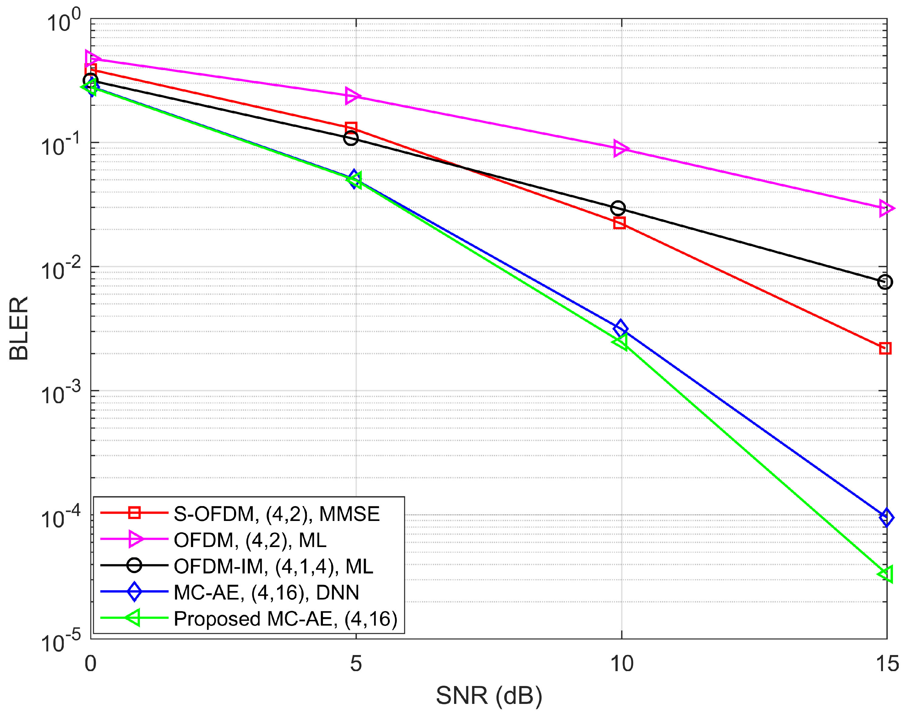
In Figure 9, the performance of the proposed model configured as (4, 16), is evaluated against ML-based OFDM and OFDM-IM, MMSE-based S-OFDM, and the DNN-based MC-AE [32] system under ideal channel conditions at a spectral efficiency (SE) of 1 bps/Hz. The results indicate that the proposed GRU-MC-AE model consistently outperforms the alternative models. While its performance closely aligns with that of the DNN-based MC-AE system at lower SNR levels, the proposed model demonstrates a notable gain of approximately $1.15$ dB in performance at higher SNR levels.

A comparative BER performance of the proposed model with the configuration $(4,16)$ is illustrated in Figure 10. This figure considers the results under perfect channel conditions at a SE of 1 bps/Hz. The performance of our proposed system is compared against several benchmarks, including a turbo-style DNN-based MC-AE system [33], an LSTM-based OFDM-IM system [22], a Y-BLSTM-based OFDM-IM system [23], and a greedy detector (GD)-based OFDM-IM system [49]. It is important to note that all OFDM systems are configured with a $(4,1,4)$ setup, while the turbo-style MC-AE uses a $(4,16)$ configuration. From the results, it is evident that the proposed model outperforms all other system models. Although the GRU-MC-AE model demonstrates slightly inferior performance at lower SNRs, particularly around 5 dB SNR, it exhibits approximately a 1 dB performance gain compared to the turbo MC-AE model at higher SNR levels.

The BLER performance of the GRU-MC-AE model under uncertain channel conditions is presented in Figure 11, using a configuration of $(4,16)$ and a training SNR of 7 dB. The figure compares the performance of the GRU-MC-AE system with a DNN-based MC-AE system, as well as ML-based OFDM, OFDM-IM, and S-OFDM systems, at a SE of 1 bps/Hz. It is important to highlight that the proposed approach is evaluated using MMSE-based imperfect CSI, despite being trained under perfect CSI conditions. As shown, the GRU-MC-AE model surpasses all other systems. While it effectively outperforms S-OFDM and the DNN-based MC-AE, it exhibits a more significant advantage over OFDM and OFDM-IM systems. Notably, at 15 dB SNR, the proposed model offers approximately a 0.7 dB improvement over the DNN-based MC-AE system and 0.9 dB improvement over the ML-based S-OFDM system.

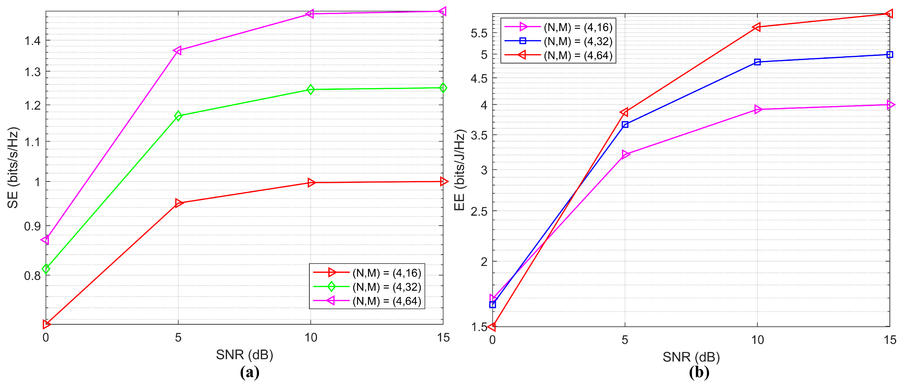
Figure 12 shows two plots that analyze the performance of a system in terms of SE and EE as a function of SNR under perfect channel conditions for different data settings. This performance is calculated with a training SNR of 7 dB, assuming a fixed circuit power of 0.25 W [50]. In Figure 12a on the left, SE is plotted against SNR for three different configurations of $(N,M)$: (4, 16), (4, 32), and (4, 64). As SNR increases, SE improves for all configurations, indicating that higher SNR values support higher data rates. Among the configurations, $(N,M)$ = (4, 64) achieves the highest SE, followed by (4, 32) and (4, 16), suggesting that the increase of M enhances SE. In Figure 12b on the right, EE is plotted against SNR for the same configurations. EE also improves with SNR, showing that the system becomes more energy-efficient at higher SNR levels. Here, the configuration $(N,M)$ = (4, 64) shows superior EE performance across most SNR values, particularly at higher SNRs. This suggests that larger values of M contribute to higher EE as well. The (4, 32) configuration follows in EE performance, and (4, 16) has the lowest EE across the SNR range. These plots provide insights into how adjusting the $(N,M)$ parameters and SNR affects the SE and EE, helping to optimize the system’s performance based on specific requirements.

5. Computational Complexity

The high computational cost of data decoding is a major challenge in today’s advanced MC systems, often viewed as a trade-off for performance enhancement. To address this, we analyze the decoding complexity of the proposed DL-based MC schemes by measuring the decoding runtime per sample and comparing it with baseline models included in Figure 9. The transmitter complexity of our schemes is minimal compared to the receiver since the proposed encoders require only a single linear fully connected layer. The decoding complexity of the proposed MC-AE and the baselines, as shown in Figure 9, is compared in

Table 2. Computational complexity comparison of the proposed GRU-based MC-AE system with other systems.

Model Name	Complexity per Sample (ms)
OFDM [9]	0.032
S-OFDM [10]	0.121
OFDM-IM [11]	0.107
DNN-based MC-AE [32]	0.028
Proposed MC-AE	0.049

, where the runtime is expressed in milliseconds (ms). Our proposed model achieves a runtime of 0.049 ms per sample. In comparison, the runtimes for S-OFDM and OFDM-IM are 0.121 ms and 0.107 ms per sample, respectively, which are significantly higher than our proposed model. Additionally, we have calculated the training time per sample for different training SNRs to further evaluate the system’s efficiency, as presented in

Table 3. Computational complexity of the proposed GRU-based MC-AE system evaluated for various training SNRs.

Training SNR (dB)	Complexity per Sample (ms)
5	0.04995
7	0.049
10	0.0517
15	0.05281

. From the table, it is evident that the runtime shows slight variations with changes in the training SNR value. While our model requires slightly more runtime than the OFDM and DNN-based MC-AE systems, the results clearly indicate that our scheme not only offers higher reliability but also benefits from lower computational complexity.

During the inference (decoding) phase of the MC-AE model, computational costs are minimized through several optimizations. The channel layer, which simulates noise and fading, leverages batch operations in TensorFlow to efficiently compute the effects of the noisy channel with parallel processing. The decoder, which uses GRU layers, is less resource-intensive, helping reduce latency. Additionally, GPU acceleration further improves performance. For class prediction, the use of $argmax$ efficiently maps probabilities to the predicted modulation classes, minimizing post-processing time.

6. Discussion

To optimize diversity and coding gains over fading channels in a fully data-driven manner, we proposed a robust DL-based MC-AE system capable of learning both the encoder and decoder. The encoder uses a linear activation function for continuous outputs, while the decoder employs a GRU neural network to effectively manage temporal dependencies across subcarriers, enhancing the system’s adaptability to varying channel conditions. In our investigation, we focused on evaluating the performance of the model, calculating key metrics such as BER, BLER, SE, and EE for different data configurations and DL model parameters. The results were compared with several conventional and DL-based models. While our system demonstrated superior performance in terms of these metrics, it exhibits higher complexity compared to some of the other models. Some techniques like model quantization, static graph execution, and simplifying the channel model through approximations for noise and fading can be employed to optimize performance while reducing complexity. These combined approaches enable faster inference with minimal performance loss. In a prior study [32], the authors designed an AE model with a DNN network and analyzed the BER and BLER for different scenarios, such as uplink-downlink and multiuser systems. Although this approach had lower complexity than ours, our model outperformed it in terms of performance. We intentionally avoid training with negative SNR levels, as excessive noise would overpower the signal, leading to overfitting and reduced information for learning. Our current work primarily focuses on static channel conditions, although we have explored varying training SNR values to account for dynamic channel conditions. Further work could extend this model to fully dynamic channel scenarios.

7. Conclusions

We proposed a robust GRU-based MC-AE system that optimizes diversity and coding gains over fading channels in a data-driven manner. We evaluated the BLER under both perfect and imperfect CSI conditions, comparing the performance of our proposed model with traditional and DL-based MC systems. Additionally, we assessed the BER performance under perfect CSI conditions. For further analysis, we calculated the SE and EE across varying SNR levels. Our findings show that the model performs optimally with a learning rate of 0.001, but it is capable of learning efficiently at different learning rates. Training at moderate SNR values helps capture more relevant features, improving generalization. Our proposed model exhibited superior performance with 1000 epochs and a batch size of 512, achieving optimal results when configured with (4, 16) and trained at 7 dB SNR. The results demonstrate that MC-AE outperforms conventional baselines, including recent IM-based and S-OFDM-based schemes, in terms of performance improvements. It also achieves superior performance compared to other DL-based OFDM-IM and MC-AE systems under both perfect and imperfect CSI conditions. Moreover, the SE and EE performance highlights the system’s robustness. Our study is primarily simulation-based, and we have not pursued practical implementation at this stage. However, in the future, the research community may consider the design of this experiment for practical implementation.