Advanced Model with a Trajectory Tracking Stabilisation System and Feasible Solution of the Optimal Control Problem

Abstract

In this study, we consider the extended optimal control problem and search for a control function in the class of feasible functions for a real control object. Unlike the classical optimal control problem, the control function should depend on the state, not time. Therefore, the control synthesis problem for the initial-state domain should be solved, instead of the optimal control problem with one initial state. Alternatively, an optimal trajectory motion stabilisation system may be constructed. Both approaches—control and trajectory motion stabilisation system syntheses—cannot be applied to real-time control, as the task is too complex. The minimum threshold of quality criteria is searched for in the space of mathematical expression codes. Among other problems, the search space is difficult to define and the gradient is hard to determine. Therefore, the advanced control object model is used to obtain a feasible control function. The advanced model is firstly obtained before solving the optimal control problem and it already includes a trajectory motion stabilisation system; in particular, this stabilisation system is synthesised in advance at the control system design stage. When the optimal control problem appears, it is solved in real time in the classical statement, and a control function is searched for as a function of time. The advanced control object model also uses the reference model to generate the optimal trajectory. The search for the optimal control function is performed in real time and considers the synthesised stabilisation system of motion along a determined trajectory. Machine learning control via symbolic regression, namely, the network operator method, is used to directly solve the control synthesis problem. An example solution of the optimal control problem, with an advanced model moving in the environment with obstacles for a group of two mobile robots, is presented. The obtained solution is a control function for a reference model that generates a trajectory from a class of trajectories stabilised with the object’s control system.

1. Introduction

This study is devoted to developing numerical methods for solving complex tasks in control theory, namely, the control synthesis problem. To implement the optimal control problem solution for a real control object, solving the control synthesis problem is necessary, which is a highly time-consuming computational task. Previous studies have proposed automatically solving this problem using effective machine learning (ML) methods [1].

Solving the optimal control problem in a classical statement leads to obtaining control as a time function. This control cannot be directly implemented for a real control object because the model of this optimal control problem was formulated and solved, as it is sensitive to the initial state and perturbations. To directly implement the optimal control problem solution in a real control object, a stabilisation system must be built for the control object’s motion along the optimal trajectory, in order to compensate for deviation from the optimal trajectory [2,3,4].

Trajectory tracking is a common motion control problem in which the control object moves with the time-parameterised reference [5,6]. Trajectory tracking is widely applied in autonomous driving [7,8], robotics [9], high-precision agriculture [10,11], and so on. Effective methods for trajectory tracking include model predictive control [12], backstepping [13], PID regulators [14], and neural network PID control [15], among others.

It should be noted that the stabilisation system should provide trajectory tracking in the expanded space of states, taking into account the time; otherwise, the value of the quality criterion obtained from solving the optimal control problem will change.

Building a trajectory motion stabilisation system is not any easier than solving the optimal control problem. It requires searching for a control function that depends on the control object’s state deviation from a given trajectory. For example, if this problem is defined as optimisation (i.e., the minimisation of deviation from a given trajectory), then its solution generally involves finding the structure and parameters of the stabilisation system function.

The search for mathematical expressions occurs in various tasks, such as experimental data approximation, inverse function searches, common differential equation solutions, control object model identification, control synthesis, and so on, and includes determining the mathematical expression in the following form:

$$\mathbf{g}(\mathbf{x},\mathbf{q}),$$

(1)

where $\mathbf{x}$ is a vector of variables, and $\mathbf{q}$ is a vector of parameters searched for with the structure of Expression (1).

Machine learning methods to search for mathematical expressions, including symbolic regression, are described in [1,16,17,18]. Symbolic regression methods allow us to determine mathematical expressions, including their parameters, using a computational evolutionary approach. The mathematical expressions are iteratively composed of alphabets of elementary functions, and the evolutionary technique is used to search for the most suitable equation to satisfy the given quality criteria. In our research, symbolic regression was applied to the control synthesis problem solution.

1.1. Relation to the Literature

The classical statement of the optimal control problem has been expanded [19], and additional optimal trajectory conditions have been introduced as the classical statement does not address stabilisation system construction for control object motion along the optimal trajectory, and creating such a stabilisation system or similar solutions is necessary to implement the optimal control problem solution. In the extended statement, obtaining an optimal control and trajectory in the state space is followed by creating a system that stabilises the control object motion along the obtained optimal trajectory. The obtained stabilisation system should ensure the attraction property in the vicinity of the optimal trajectory. However, a quality problem arises when synthesising a motion stabilisation system, as the criterion of reducing the motion error along a given trajectory is usually used.

The main issue in solving the extended optimal control problem is that the stabilisation system for object motion along the optimal trajectory significantly changes the mathematical model of the control object. Initially, the optimal control problem was deemed to be solved for one mathematical model of the control object. In reality, the object moving along the trajectory had another mathematical model that was overlooked at first. Another issue is that the motion stabilisation system cannot be synthesised on the on-board processor of the control object in real time. If the optimal control problem can be solved via the direct method on the on-board processor of the control object within a few seconds, then synthesis of the motion stabilisation system requires much more time due to its computational complexity.

The authors of [20] presented a universal stabilisation system for motion along a given trajectory. Initially, several trajectories were set in the state space, and one universal stabilisation system was sought, which ensured control object motion in the vicinity of all given trajectories. Furthermore, when the optimal control problem is solved, the universal stabilisation system is used. In this study, the optimal control problem is solved in real time with a possible deterioration in the stabilisation quality of the motion along the optimal trajectory, as the obtained optimal trajectory is not guaranteed to belong to the class of trajectories that the universal stabilisation system stabilises. In addition, the second problem remains. The optimal control problem is solved for a mathematical model of the control object that does not include a stabilisation system, and a real control object contains a stabilisation system.

In the work of [21], the problem of stabilising the motion along a given trajectory was considered. The trajectory was given in space in the form of straight-line segments. A reference model of motion was created to calculate the deviation from the trajectory. For this purpose, the motion speed along each segment was calculated and considered constant. The deviation of the object from the reference motion of the point along the trajectory was calculated at each segment. To solve the control synthesis problem, the network operator method was used and a stabilisation system was obtained.

1.2. Contribution

In this study, we searched for a feasible optimal control problem solution. The search space includes a class of feasible optimal trajectories.

An advanced mathematical model of the control object was used to solve the extended optimal control problem. Initially, a universal stabilisation system was built. Furthermore, the stabilisation system was input into the mathematical model of the control object. An object trajectory vector in an extended state space in the right part of the control object model was obtained, instead of a free control vector. The mathematical model of the control object includes a reference model, which contains a free control vector in the right part. As a result, the advanced control object model was obtained. The dimension of the advanced model is twice as large as the original control object model. The advanced mathematical model allowed us to solve the optimal control problem in the classical statement, in an on-board and online manner. The optimal control problem was solved for an object with a mathematical model that includes a stabilisation system for motion along a given trajectory.

The rest of this study is organised as follows: The advanced model and problem statement of the control object are presented in Section 2; a network operator method, as one of the symbolic regression methods, is outlined in Section 3; computational experiments focused on solving the optimal control, control synthesis, and stabilisation system synthesis problems for two-wheeled robots are described in Section 4, followed by a discussion in Section 5, a conclusion in Section 6, and potential avenues for future studies in Section 7.

2. Advanced Control Object Model and Problem Statement

In the classical statement of the optimal control problem, the mathematical model of the control object is given as follows:

$$\dot{\mathbf{x}}=\mathbf{f}(\mathbf{x},\mathbf{u}),$$

(2)

where $\mathbf{x}$ is a state vector, $\mathbf{x}\in {\mathbb{R}}^n$, $\mathbf{u}$ is a control vector, $\mathbf{u}\in \mathrm{U}\subseteq {\mathbb{R}}^m$, and $\mathrm{U}$ is a compact set that, as a rule, determines constraints on the control.

The initial state is

$$\mathbf{x}\left(0\right)={\mathbf{x}}^0={[x_1^0\dots x_n^0]}^T.$$

(3)

The terminal state is

$$\mathbf{x}\left(t_f\right)={\mathbf{x}}^f={[x_1^f\dots x_n^f]}^T,$$

(4)

where $t_f$ is a terminal time, $t_f⩽t^{+}$, and $t^{+}$ is a given limitation.

The quality criterion in an integral form is

$$J_0=\underset{0}{\overset{t_f}{\int }}{f}_0(\mathbf{x},\mathbf{u})dt\to \underset{\mathbf{u}\in \mathrm{U}}{min}.$$

(5)

We created a universal stabilisation system of motion along a given trajectory to develop an advanced model. For this purpose, we formulated the problem of a universal stabilisation system synthesis. The initial state domain is given as a deviation from the specified initial state as follows:

$${\mathrm{X}}_0=\{{\mathbf{x}}^0\pm \Delta \},$$

(6)

where $\Delta ={[{\Delta }_1\dots {\Delta }_n]}^T$.

A set of diverse control functions is

$${\mathrm{V}}^{*}=\{{\mathbf{v}}^{*,1}\left(t\right),\dots ,{\mathbf{v}}^{*,M}\left(t\right)\},0⩽t⩽t^{+},$$

(7)

where

$${\mathbf{v}}^{*,j}\left(t\right)\in \mathrm{U},\forall t\in [0;t^{+}],j=1,\dots ,M.$$

(8)

The diversity of functions should be enough to consider all control object features. Functions in (7) may include simple discontinuities.

If we substitute the control functions in (7) into the right parts of the control object model (2), we can then obtain a set of program trajectories as particular solutions of the ODE system from a given initial state, as shown in the following equation:

$${\mathrm{X}}^{*}=\{{\mathbf{x}}^{*,1}(t,{\mathbf{x}}^0),\dots ,{\mathbf{x}}^{*,M}(t,{\mathbf{x}}^0)\},$$

(9)

where ${\mathbf{x}}^{*,j}(t,{\mathbf{x}}^0)$ is a particular solution of the ODE system (2) from an initial state (3) with the control function ${\mathbf{v}}^{*,j}\left(t\right)$ in the right part.

$$\dot{\mathbf{x}}=\mathbf{f}(\mathbf{x},{\mathbf{v}}^{*,j}\left(t\right)),j\in \{1,\dots ,M\}.$$

(10)

Then, we searched for control in (2) as a function of state

$$\mathbf{u}=\mathbf{h}({\mathbf{x}}^{*,j}\left(t\right)-\mathbf{x})\in \mathrm{U},j\in \{1,\dots ,M\}.$$

(11)

To minimise the following quality criterion:

$$J_1=\sum _{j=1}^M\sum _{k=0}^{2^n-1}\underset{0}{\overset{t^{+}}{\int }}\parallel {\mathbf{x}}^{*,j}\left(t\right)-\mathbf{x}(t,{\mathbf{x}}^{0,k})\parallel dt\to \underset{\mathbf{h}({\mathbf{x}}^{*,j}\left(t\right)-\mathbf{x})\in \mathrm{U}}{min},$$

(12)

where ${\mathbf{x}}^{0,k}$ is a particular solution of the ODE system,

$$\dot{\mathbf{x}}=\mathbf{f}(\mathbf{x},\mathbf{h}({\mathbf{x}}^{*,j}\left(t\right)-\mathbf{x})),$$

(13)

from the initial state of

$${\mathbf{x}}^{0,k}={\mathbf{x}}^0-\Delta +2{\left(k\right)}_2\odot \Delta ,k=0,\dots ,2^n-1,$$

(14)

where ${\left(k\right)}_2$ is a binary code of the number k of n bit, and ⊙ is a Hadamard product of vectors.

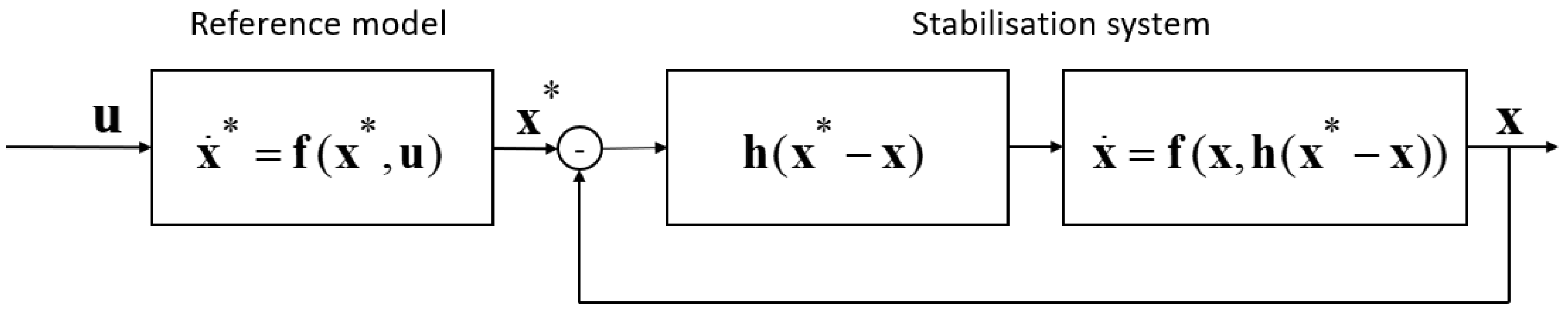
The obtained stabilisation system (11) is inserted into the mathematical model of the control object. Then, the original model (2) is added. As a result, the advanced mathematical model of the control object is obtained:

$$\begin{array}{ccc}\hfill {\dot{\mathbf{x}}}^{*}& =& \mathbf{f}({\mathbf{x}}^{*},\mathbf{u}),\hfill \\ \hfill \dot{\mathbf{x}}& =& \mathbf{f}(\mathbf{x},\mathbf{h}({\mathbf{x}}^{*}-\mathbf{x})).\hfill \end{array}$$

(15)

The structure of the advanced model (15) (see Figure 1) consists of two subsystems: the reference model, which is usually realised on the on-board processor, and a model of the control object with a trajectory tracking stabilisation system.

The first subsystem is related to the open-loop control, while the second subsystem is related to the closed-loop control. Therefore, the control quality depends on the stabilisation formula $\mathbf{h}$ previously found for a class of trajectories (9) and the initial state domain (6).

For the advanced model (15), the optimal control problem can be solved in the classical statement. A control function is found as a time function, using the quality criterion of reaching the terminal state and avoiding collisions with obstacles, namely, satisfying the phase constraints in terms of control theory. Phase constraints may be static and dynamic in nature. Static phase constraints are obstacles in the environment, and dynamic phase constraints are possible collisions between interacting objects.

The two-step scheme for designing a control system based on the proposed advanced control object model is shown in Figure 2. In the first step, a universal stabilisation system for trajectory tracking is obtained using a machine-learning symbolic regression method. In the second step, an optimal control problem is solved using an evolutionary algorithm for the advanced model. The obtained solution belongs to the class of feasible control functions.

For the advanced model, it is possible to build a Hamiltonian system of differential equations for conjugate variables and use the maximum principle

$$H({\mathbf{x}}^{*},\mathbf{x},{\psi }^{*},\psi )=-f_0(\mathbf{x},\mathbf{u})+{\mathit{\psi }}^{*T}\mathbf{f}({\mathbf{x}}^{*},\mathbf{u})+{\mathit{\psi }}^T\mathbf{f}(\mathbf{x},\mathbf{h}({\mathbf{x}}^{*}-\mathbf{x})),$$

(16)

where ${\mathit{\psi }}^{*}$ and $\mathit{\psi }$ are vectors of conjugate variables as shown in the following equations:

$${\dot{\mathit{\psi }}}^{*}=-{\displaystyle \frac{\partial H({\mathbf{x}}^{*},\mathbf{x},{\mathit{\psi }}^{*},\mathit{\psi })}{\partial {\mathbf{x}}^{*}}},$$

(17)

$$\dot{\mathit{\psi }}=-{\displaystyle \frac{\partial H({\mathbf{x}}^{*},\mathbf{x},{\mathit{\psi }}^{*},\mathit{\psi })}{\partial \mathbf{x}}}.$$

(18)

3. Machine Learning for Stabilisation System Synthesis

To solve the control synthesis problems (2), (11), (12), and (14) and obtain a stabilisation formula $\mathbf{h}$ for a class of trajectories (9), machine learning control via symbolic regression was used.

Symbolic regression encodes mathematical expressions as special codes and searches for the solution in the code space. The space of mathematical expression codes is not numerical, and it is rather difficult to determine the search direction as it does not have the metrics to estimate the distance between possible solutions nor a possible solution to evaluate the gradient. The convergence of symbolic regression algorithms is the main problem in this optimisation class. Let us call this class non-numeric. It contains the most difficult optimisation problems. A developed search algorithm should, at least, guarantee more efficient performance than a simple random search.

To assess the distance between two possible solutions in the space of mathematical expression codes, the concept of small variation in the mathematical expression code is defined in [22]. As most codes of mathematical expressions are integer mathematical constructions, vectors, matrices, sets, and so on, a small variation in code means the smallest number of integer changes in a mathematical construction code (i.e., their positions and values). With this small change in code, the correct code of another mathematical expression should be obtained. Any symbolic regression method has its own set of small variations.

Any mathematical expression may have an infinite number of representations if any other expression that can be added to the outlined expression is also equal to zero. However, as a rule, mathematical expressions are written in the most compact form possible, without adding identical expressions equal to zero or multiplying by mathematical expressions with identical unit values.

When searching for a mathematical expression in the code space, it is difficult to state that the found code does not contain insignificant additives. Therefore, it is necessary to limit the length of the searched code. Small variations must possess the property of completeness. This means that any mathematical expression described using symbolic regression code from a set of codes of limited length can be transformed using a finite number of small variations into any other mathematical expression with code belonging to the same set.

$$\tilde{\mathsf{\Psi }}=\mathsf{\Psi }\circ {\mathbf{w}}^1\circ \cdots \circ {\mathbf{w}}^d,$$

(19)

where $\mathsf{\Psi }$ is a code of initial mathematical expression, ${\mathbf{w}}^i$ is a code of small variation, d is a number of small variations, $\tilde{\mathsf{\Psi }}$ is a code of a new mathematical expression, and ∘ denotes an operator of the variation application.

We considered an example of encoding a mathematical expression and applying small variations. To code mathematical expressions, we used a graph-based structure of a network operator (for more details, see [18]). Then, we needed to code and vary the following mathematical expression:

$$y=e^{(-q_1{x}_1)}cos(q_2{x}_2+q_1)$$

(20)

where $x_1$, $x_2$ are variables, and $q_1$, $q_2$ are constant parameters.

To code the mathematical expression, an alphabet of unary and binary functions was used.

Unary functions include the following:

$${\mathrm{F}}_1=\{f_{1,1}\left(z\right)=z,f_{1,2}\left(z\right)=exp\left(z\right),f_{1,3}\left(z\right)=-z,f_{1,4}\left(z\right)=cos\left(z\right)\}.$$

(21)

Binary functions include the following:

$${\mathrm{F}}_2=\{f_{2,1}(z_1,z_2)=z_1+z_2,f_{2,2}(z_1,z_2)=z_1·z_2\}.$$

(22)

The identity function $f_{1,1}\left(z\right)$ is obligatory in Equation (21). Binary functions in Equation (22) should be commutative and associative and have a unit element: 0 for addition and 1 for multiplication.

In the PC memory, the network operator is represented as the following integer matrix:

$$\mathsf{\Psi }=\left[\begin{array}{cccccccc}0& 0& 0& 0& 1& 0& 0& 0\\ 0& 0& 0& 0& 3& 0& 1& 0\\ 0& 0& 0& 0& 0& 1& 0& 0\\ 0& 0& 0& 0& 0& 1& 0& 0\\ 0& 0& 0& 0& 2& 0& 0& 2\\ 0& 0& 0& 0& 0& 2& 1& 0\\ 0& 0& 0& 0& 0& 0& 1& 4\\ 0& 0& 0& 0& 0& 0& 0& 2\end{array}\right].$$

(23)

In the matrix, rows that have zeroes on the main diagonal are connected to source nodes (variables and parameters). Other elements on the main diagonal are numbers from (22). The elements above the main diagonal are numbers from (21). For coding and decoding algorithms, see [18].

Let us apply the principle of small variations and varied expression (20) using two small variations, ${\mathbf{w}}^1$ and ${\mathbf{w}}^2$, as outlined in the following equation:

$$\tilde{\mathsf{\Psi }}=\mathsf{\Psi }\circ {\mathbf{w}}^1\circ {\mathbf{w}}^2,{\mathbf{w}}^1={\left[2471\right]}^T,{\mathbf{w}}^2={\left[3270\right]}^T.$$

(24)

The first component in the vector of variation is a code of small variation types: 0—alternation of unary function; 1—alternation of binary function; 2—addition of unary function; 3—deletion of unary function. The second and third components are numbers of rows and columns in the matrix. The fourth component is a number of the unary or binary function depending on the type of variation.

Having performed two variations, we obtained a new matrix of the network operator and, thus, a new mathematical expression as follows:

$$\tilde{\mathsf{\Psi }}=\left[\begin{array}{cccccccc}0& 0& 0& 0& 1& 0& 0& 0\\ 0& 0& 0& 0& 3& 0& 0& 0\\ 0& 0& 0& 0& 0& 1& 0& 0\\ 0& 0& 0& 0& 0& 1& 1& 0\\ 0& 0& 0& 0& 2& 0& 0& 2\\ 0& 0& 0& 0& 0& 2& 1& 0\\ 0& 0& 0& 0& 0& 0& 1& 4\\ 0& 0& 0& 0& 0& 0& 0& 2\end{array}\right]$$

(25)

$$y=e^{(-q_1{x}_1)}cos(q_2{x}_2+q_2).$$

(26)

4. Computational Experiment

A series of computational experiments were carried out.

4.1. Optimal Control Problem

We considered the optimal control problem for two-wheeled differential drive robots.

The mathematical model of control object is given as follows:

$$\begin{array}{ccc}\hfill {\dot{x}}_1^j& =& 0.5(u_1^{\left(j\right)}+u_2^{\left(j\right)})cos\left(x_3^{\left(j\right)}\right),\hfill \\ \hfill {\dot{x}}_2^j& =& 0.5(u_1^{\left(j\right)}+u_2^{\left(j\right)})sin\left(x_3^{\left(j\right)}\right),\hfill \\ \hfill {\dot{x}}_3^j& =& 0.5(u_1^{\left(j\right)}-u_2^{\left(j\right)}),\hfill \end{array}$$

(27)

where j is an index of the robot $j=1,2$, ${\mathbf{x}}^j={\left[x_1^{\left(j\right)}{x}_2^{\left(j\right)}{x}_3^{\left(j\right)}\right]}^T\in {\mathbb{R}}^n$, ${\mathbf{u}}^j={\left[u_1^{\left(j\right)}{u}_2^{\left(j\right)}\right]}^T\in \mathrm{U}\subseteq {\mathbb{R}}^m$, and $\mathrm{U}$ is a compact set that is determined by constraints on control:

$$-10=u_i^{-}⩽u_i^{\left(j\right)}⩽u_i^{+}=10,i=1,2.$$

(28)

The initial states of both robots are given as follows:

$${\mathbf{x}}^1\left(0\right)={\mathbf{x}}^{0,1}={\left[000\right]}^T,{\mathbf{x}}^2\left(0\right)={\mathbf{x}}^{0,2}={\left[1010\pi \right]}^T.$$

(29)

The terminal states are given as follows:

$${\mathbf{x}}^1\left(t_f\right)={\mathbf{x}}^{f,1}={\left[10100\right]}^T,{\mathbf{x}}^2\left(t_f\right)={\mathbf{x}}^{f,2}={\left[00\pi \right]}^T,$$

(30)

where $t_f$ is a time to reach the terminal states by each of the robots, $t_f$ is not given but limited by $t_f⩽t^{+}$, and $t^{+}$ is a given limited time. If two robots reach their terminal states at different times $t_{f,1}⩽t^{+}$, $t_{f,2}⩽t^{+}$, then a maximal time is considered as follows:

$$t_f=max\{t_{f,1},t_{f,2}\}.$$

(31)

Static phase constraints are given in the form of circular obstacles as follows:

$${\phi }_i\left({\mathbf{x}}^j\right)=r_i-\sqrt{{(x_{1,i}-x_1^{\left(j\right)})}^2+{(x_{2,i}-x_2^{\left(j\right)})}^2}⩽0,i=1,2,j=1,2,$$

(32)

where $r_1=2$, $r_2=2$, $x_{1,1}=2$, $x_{2,1}=5$, $x_{1,2}=8$, and $x_{2,2}=5$.

Dynamic phase constraints consider collision avoidance conditions as follows:

$$\chi ({\mathbf{x}}^1,{\mathbf{x}}^2)=r_0-\sqrt{{(x_1^{\left(1\right)}-x_1^{\left(2\right)})}^2+{(x_2^{\left(1\right)}-x_2^{\left(2\right)})}^2}⩽0,$$

(33)

where $r_0=1.5$.

It is necessary to find a control function with respect to constraints (28) in order to reach the terminal states and minimise the following quality criterion:

$$J_2=\underset{0}{\overset{t_f}{\int }}1dt=t_f\to \underset{{\mathbf{u}}^1,{\mathbf{u}}^2\in \mathrm{U}}{min}.$$

(34)

Firstly, the optimal control problem is solved in the classical statement, and the control function is a function of time. For this purpose, the direct approach is used. According to this approach, phase constraints and the accuracy of reaching the terminal states are included in the quality criterion as follows:

$$\begin{array}{c}{J}_3=t_f+{\displaystyle \sum _{j=1}^2}\left(p_1\parallel {\mathbf{x}}^{j,f}-{\mathbf{x}}^j\left(t_{f,j}\right)\parallel +p_2\underset{0}{\overset{t_{f,j}}{\int }}{\displaystyle \sum _{i=1}^2}\vartheta \left({\phi }_i\left({\mathbf{x}}^j\right)\right)dt\right)+\\ p_3\underset{0}{\overset{t_f}{\int }}\vartheta \left(\chi ({\mathbf{x}}^1,{\mathbf{x}}^2)\right)dt\to \underset{{\mathbf{u}}^1,{\mathbf{u}}^2\in \mathrm{U}}{min},\end{array}$$

(35)

where $p_1=1$, $p_2=3$, and $p_3=3$ are penalty coefficients.

$$t_{f,j}=\left\{\begin{array}{c}t,\mathrm{if}t<t^{+}\mathtt{and}\parallel {\mathbf{x}}^{j,f}-{\mathbf{x}}^j\left(t\right)\parallel ⩽\epsilon \hfill \\ t^{+},\mathrm{otherwise}\hfill \end{array}\right.,j=1,2,$$

(36)

$\epsilon =0.05$, and $t^{+}=1.8$, $\vartheta \left(\alpha \right)$ is a Heaviside function

$$\vartheta \left(\alpha \right)=\left\{\begin{array}{c}1,\mathrm{if}\alpha >0\hfill \\ 0,\mathrm{otherwise}\hfill \end{array}\right..$$

(37)

The control function is found in the form of a piece-wise linear approximation of the time function. The time axis is divided into equal intervals $\Delta t$ and on the borders of intervals; the values of constant parameters are found for the respective control of both robots. Within the intervals, the parameter values are linked by straight lines. The control function is truncated at the top and bottom according to the specified control constraints in the following:

$$u_i^{\left(j\right)}=\left\{\begin{array}{c}{u}_i^{+},\mathrm{if}{u}_i^{+}⩽v_i^{\left(j\right)}\left(t\right)\hfill \\ u_i^{-},\mathrm{if}{v}_i^{\left(j\right)}\left(t\right)⩽u_i^{-}\hfill \\ v_i^{\left(j\right)},\mathrm{otherwise}\hfill \end{array}\right.,i=1,2,j=1,2,$$

(38)

where

$$v_i^{\left(j\right)}=\left({\tilde{q}}_{i+(k-1)mN}\right)+({\tilde{q}}_{i+kmN}-{\tilde{q}}_{i+(k-1)mN}){\displaystyle \frac{t-k\Delta t}{\Delta t}},$$

(39)

$(k-1)\Delta T⩽t<k\Delta t$, $k=1,\dots ,L$, m is a number of components in the control vector, $m=2$, N is a number of robots, $N=2$, $\Delta t$ is a time interval, $\Delta t=0.2$, and L is a number of intervals.

$$L=⌊{\displaystyle \frac{t^{+}}{\Delta t}}⌋=⌊{\displaystyle \frac{1.8}{0.2}}⌋=9.$$

(40)

Thus, an optimal control problem solution (27)–(30), (35) includes a vector of constant parameters

$$\tilde{\mathbf{q}}={[{\tilde{q}}_1\dots {\tilde{q}}_{(L+1)mN}]}^T={[{\tilde{q}}_1\dots {\tilde{q}}_{40}]}^T.$$

(41)

To numerically solve the optimal control problem, a hybrid evolutionary algorithm was used [23]. The algorithm includes evolutionary transformations from three evolutionary algorithms: the genetic algorithm, particle swarm optimisation, and the grey wolf optimiser.

The hybrid algorithm determined the following solution:

$$\begin{array}{ccc}\hfill \tilde{\mathbf{q}}& =& [16.7976-4.891716.9660-9.20932.55605.618714.65278.5727\hfill \\ \hfill & & 15.763617.262319.998716.332114.74981.2650-1.240719.8177\hfill \\ \hfill & & 14.955319.274919.9999-6.249918.02103.140215.886319.9450\hfill \\ \hfill & & 0.721818.036116.344818.280718.224816.78533.318817.0318\hfill \\ \hfill & & {11.568210.324611.194916.7666-19.408914.1827-5.288617.9824]}^T.\hfill \end{array}$$

(42)

Figure 3 shows the optimal trajectories of two robots. The red circles are obstacles or static phase constraints in terms of control theory. As shown in Figure 3, the found solution is almost optimal because both robots avoided collisions, satisfied the phase constraints, and reached the given terminal states. The quality criterion value of (35) was $J_3=1.8003$.

The solution in the form of the control function of time cannot be implemented in real objects since the control system is open-loop. If the initial conditions change, the obtained optimal control will no longer remain optimal even in a small domain.

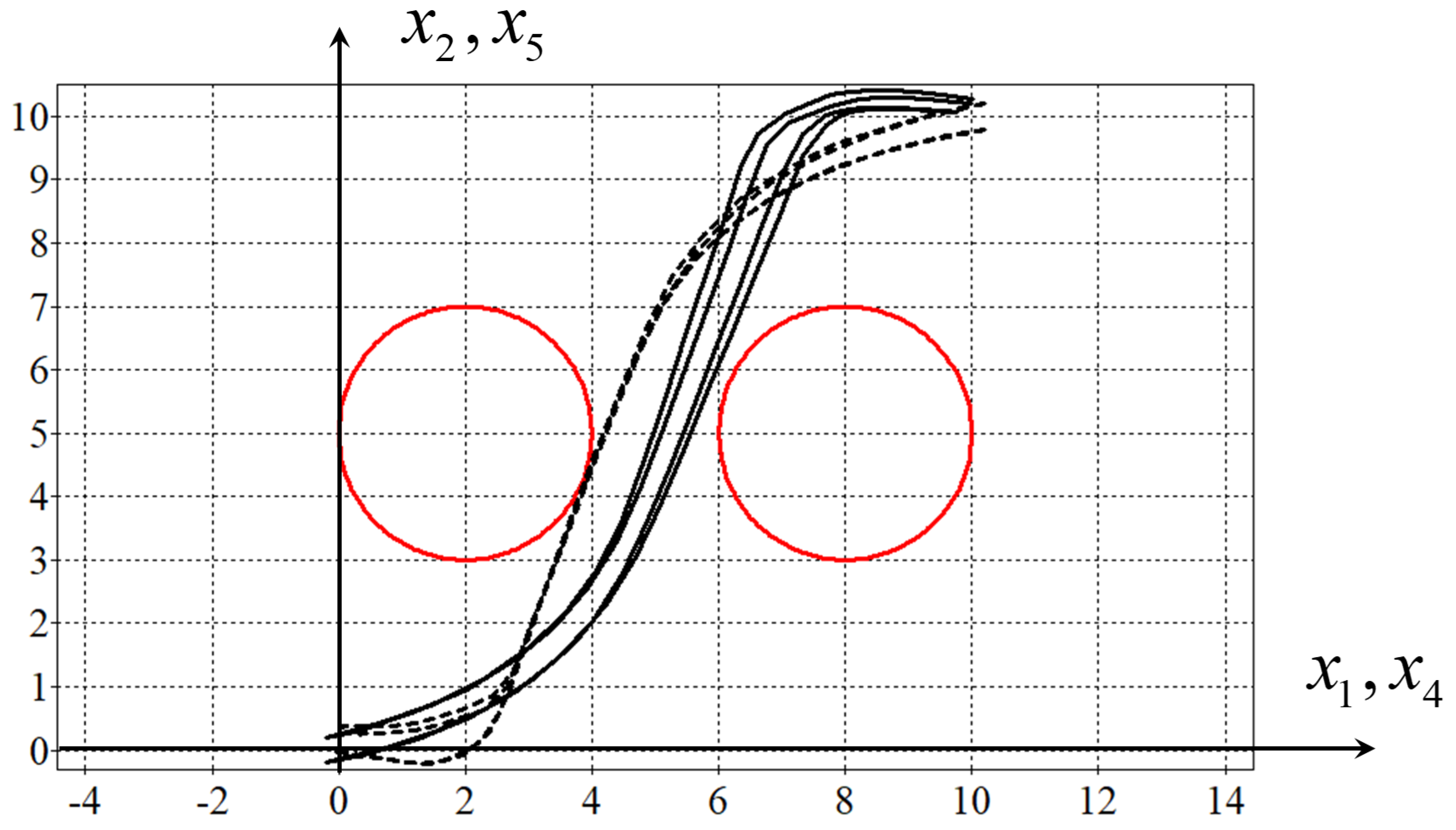
Figure 4 shows robots trajectories from four randomly disturbed initial states in the range of ${\Delta }_0=\pm 0.2$, as shown in the following:

$$x_i^{\left(j\right)}\left(0\right)=x_i^{j,0}+(2\xi \left(t\right)-1){\Delta }_0,i=1,2,3,j=1,2,$$

(43)

where $\xi \left(t\right)$ is a generator of random numbers that returns a random value from 0 to 1 at every call. Small disturbances of the initial states essentially change the trajectories. The robots violate phase constraints and do not reach terminal states. The average value of (35) in a series of 10 experiments was $J_3=6.51$. To deal with this problem, we proposed to solve the optimal control problem as a control synthesis problem.

4.2. Control Synthesis Problem

In the control synthesis problem, mathematical models of two robots should be considered as a model of one control object because a control function of one robot depends on the state vector of the other.

The mathematical model of control object is

$$\begin{array}{ccc}\hfill {\dot{x}}_1& =& 0.5(u_1+u_2)cos\left(x_3\right),\hfill \\ \hfill {\dot{x}}_2& =& 0.5(u_1+u_2)sin\left(x_3\right),\hfill \\ \hfill {\dot{x}}_3& =& 0.5(u_1-u_2),\hfill \\ \hfill {\dot{x}}_4& =& 0.5(u_3+u_4)cos\left(x_6\right),\hfill \\ \hfill {\dot{x}}_5& =& 0.5(u_3+u_4)sin\left(x_6\right),\hfill \\ \hfill {\dot{x}}_6& =& 0.5(u_3-u_4),\hfill \end{array}$$

(44)

where $x_1$, $x_2$, and $x_3$ are coordinates of the state vector of the first robot; $x_4$, $x_5$, and $x_6$ are coordinates of the state vector of the second robot; $u_1$ and $u_2$ are components of the control vector of the first robot; and $u_3$ and $u_4$ are components of the control vector of the second robot.

The constraints on control are

$$-10=u_i^{-}⩽u_i⩽u_i^{+}=10,i=1,\dots ,m=4.$$

(45)

The terminal state is

$$\mathbf{x}\left(t_f\right)={\mathbf{x}}^f={\left[1010000\pi \right]}^T,$$

(46)

where $t_f$ is not given but limited $t_f⩽t^{+}=2.2$.

A set of initial states is given in the form of the $\Delta$ neighbourhood of the original initial state for the optimal control problem

$$\mathbf{x}\left(0\right)\in {\mathrm{X}}_0=\{{\mathbf{x}}^0\pm {\Delta }_0\},$$

(47)

where

$$\begin{array}{ccc}\hfill {\mathbf{x}}^0& =& {\left[0001010\pi \right]}^T,\hfill \\ \hfill {\Delta }_0& =& {[0.20.2\pi /180.20.2\pi /18]}^T.\hfill \end{array}$$

(48)

For the numerical solution of the synthesis problem, the domain of initial states is replaced by a set of points

$${\tilde{\mathrm{X}}}_0=\{{\mathbf{x}}^{0,i}:i=1,\dots ,K\},$$

(49)

where

$${\mathbf{x}}^{0,i}=({\mathbf{x}}^0-{\Delta }_0)+\mathbf{i}\odot 2{\Delta }_0,$$

(50)

$\mathbf{i}$ is an integer binary vector of two binary vectors, three bits each, as shown in the following equation:

$$\mathbf{i}={[{(i-1)}_2⋮{(i-1)}_2]}^T,i=1,\dots ,2^{2n/2}=8,$$

(51)

${(i-1)}_2$ is a three bit binary code of the number $i-1$, and ⊙ is a Hadamard or element-wise product of vectors.

The quality criterion is

$$\begin{array}{c}{J}_4={\displaystyle \sum _{i=1}^K}\left(t_{f,i}+p_1\parallel {\mathbf{x}}^f-\mathbf{x}(t_{f,i},{\mathbf{x}}^{0,i})\parallel +p_2\underset{0}{\overset{t_{f,i}}{\int }}\vartheta \left(\tilde{\chi }\left(\mathbf{x}(t,{\mathbf{x}}^{0,i})\right)\right)dt+\right.\\ \left.p_3\underset{0}{\overset{t_f}{\int }}{\displaystyle \sum _{j=1}^2}\left(\vartheta \left({\alpha }_j\left(\mathbf{x}(t,{\mathbf{x}}^{0,i})\right)\right)+\vartheta \left({\beta }_j\left(\mathbf{x}(t,{\mathbf{x}}^{0,i})\right)\right)\right)dt\right)\to \underset{\mathbf{u}}{min},\end{array}$$

(52)

where $\mathbf{x}(t,{\mathbf{x}}^{0,i})$ is a particular solution of the ODE system (44) from the initial state ${\mathbf{x}}^{0,i}$, $i\in \{1,\dots ,8\}$, and $p_1=1$, $p_2=3$, and $p_3=3$ are penalty coefficients.

$$t_{f,i}=\left\{\begin{array}{c}t,\mathrm{if}t<t^{+}\mathtt{and}\parallel {\mathbf{x}}^f-\mathbf{x}(t,{\mathbf{x}}^{0,i})\parallel ⩽{\epsilon }_0\hfill \\ t^{+},\mathrm{otherwise}\hfill \end{array}\right.,$$

(53)

${\epsilon }_0=0.05$, $t^{+}=2.4$,

$${\alpha }_j\left(\mathbf{x}\right)=r_j-\sqrt{{(x_{1,j}-x_1)}^2+{(x_{2,j}-x_2)}^2},$$

(54)

$${\beta }_j\left(\mathbf{x}\right)=r_j-\sqrt{{(x_{1,j}-x_4)}^2+{(x_{2,j}-x_5)}^2},$$

(55)

$j=1,2$, $r_1=2$, $x_{1,1}=2$, $x_{2,1}=5$, $r_2=2$, $x_{1,2}=8$, $x_{2,2}=5$,

$$\tilde{\chi }\left(\mathbf{x}\right)=r_0-\sqrt{{(x_1-x_4)}^2+{(x_2-x_5)}^2},$$

(56)

$r_0=1.25$.

In the control synthesis problem, it is necessary to find a control function as a function of the state space vector as follows:

$$\mathbf{u}=\mathbf{g}({\mathbf{x}}^f-\mathbf{x}).$$

(57)

If the control function (57) is placed in the right part of the ODE system (44), then the system will have a particular solution from any initial state of (47) that will reach the given terminal state (46) with an optimal value of the quality criterion (52).

The control synthesis problem may be effectively solved using symbolic regression methods. Here, the network operator method was applied.

The network operator method was performed with the following parameters: an NOP matrix size of $32\times 32$, 12 source nodes for the NOP graph, including 6 nodes for variables and 6 nodes for searched parameters, and 4 sink nodes for the output components of the control vector. The variational genetic algorithm parameters were as follows: the number of possible solutions in the initial population—1024; the number of crossover operations in one generation—128; the number of generations—128; the depth of variation—7; the number of generations between change in the basic solution—20; the number of bits for coding a parameter—16.

Computations were performed on a CPU Intel core i7, 2.8 GHz. The computational time was approx. 10 min. Any change in the obstacle position required recalculation. It could be completed offline on on-board processors but not in real time.

The following solution was obtained using the network operator method as follows:

$$u_i=g_i({\mathbf{x}}^f-{\mathbf{x}}^j)=\left\{\begin{array}{c}{u}_i^{+},\mathrm{if}{u}_i^{+}⩽{\tilde{g}}_i({\mathbf{x}}^f-\mathbf{x})\hfill \\ u_i^{-},\mathrm{if}{\tilde{g}}_i({\mathbf{x}}^f-\mathbf{x})⩽u_i^{-}\hfill \\ {\tilde{g}}_i({\mathbf{x}}^f-\mathbf{x}),\mathrm{otherwise}\hfill \end{array}\right.,i=1,2,3,4,$$

(58)

where

$${\tilde{g}}_1({\mathbf{x}}^f-\mathbf{x})=(F-E)ln\left(\right|F\left|\right)arctan(C+{\rho }_3\left(q_6\right)+\mu \left(q_5\right))\mathrm{sgn}\left(C\right)\sqrt{\left|C\right|},$$

(59)

$$\begin{array}{c}{\tilde{g}}_2({\mathbf{x}}^f-\mathbf{x})=H+\mu \left(F\right)+{\rho }_1\left(E\right)+\vartheta \left(D\right)+{\rho }_2\left(q_2(x_2^f-x_2)\right)+\\ {\left(q_1(x_1^f-x_1)\right)}^{-1}+{\rho }_2\left(q_6\right)+q_1^{-1}+\mu (x_5^f-x_5)+{\rho }_2(x_1^f-x_1),\end{array}$$

(60)

$${\tilde{g}}_3({\mathbf{x}}^f-\mathbf{x})={\tilde{g}}_1({\mathbf{x}}^f-\mathbf{x}),$$

(61)

$$\begin{array}{c}{\tilde{g}}_4({\mathbf{x}}^f-\mathbf{x})=cos\left({\tilde{g}}_3({\mathbf{x}}^f-\mathbf{x})\right)+{\tilde{g}}_2({\mathbf{x}}^f-\mathbf{x})+{\left({\tilde{g}}_1({\mathbf{x}}^f-\mathbf{x})\right)}^{-1}+\\ {\rho }_2\left(H\right)+{\rho }_2\left(q_4\right)+{\rho }_2(x_5^f-x_5),\end{array}$$

(62)

$$A=tanh\left(q_2(x_2^f-x_2)\right)q_5(x_5^f-x_5),$$

$$B=q_6(x_6^f-x_6)\mathrm{sgn}(x_1^f-x_1)\sqrt{|x_1^f-x_1|},$$

$$C=exp\left(A\right)+q_3(x_3^f-x_3)+q_2(x_2^f-x_2)+q_1(x_1^f-x_1),$$

$$D=B+A+\sqrt[3]{q_3(x_3^f-x_3)}{q}_4(x_4^f-x_4)+exp(x_4^f-x_4),$$

$$E=\mu (C+{\rho }_3\left(q_6\right)+\mu \left(q_5\right))D{\rho }_2\left(q_6\right)\mathrm{sgn}\left(C\right)tanh\left(q_1(x_1^f-x_1)\right),$$

$$F=C+{\rho }_3\left(q_6\right)+\mu \left(q_5\right)+{\rho }_2\left(D\right)+cos\left(B\right),$$

$$G=E\mu (C+{\rho }_3\left(q_6\right))tanh\left(q_2(x_2^f-x_2)\right),$$

$$H=\vartheta (F-E)G{\rho }_3(C+{\rho }_3\left(q_6\right))arctan\left(D\right)tanh\left(C\right)\mathrm{sgn}\left(E\right)\sqrt{\left|E\right|},$$

$$\mu \left(\alpha \right)=\left\{\begin{array}{c}\alpha ,\mathrm{if}\left|\alpha \right|<1\hfill \\ \mathrm{sgn}\left(\alpha \right),\mathrm{otherwise}\hfill \end{array}\right.,{\rho }_1\left(\alpha \right)=\mathrm{sgn}\left(\alpha \right)(exp(\left|\alpha \right|)-1),$$

$${\rho }_2\left(\alpha \right)=\mathrm{sgn}\left(\alpha \right)exp(-|\alpha \left|\right),{\rho }_3\left(\alpha \right)=\mathrm{sgn}\left(\alpha \right)ln\left(\right|\alpha |+1),$$

$q_1=1.1709$, $q_2=12.27979$, $q_3=7.32666$, $q_4=4.92456$, $q_5=3.90015$, $q_6=1.73071$.

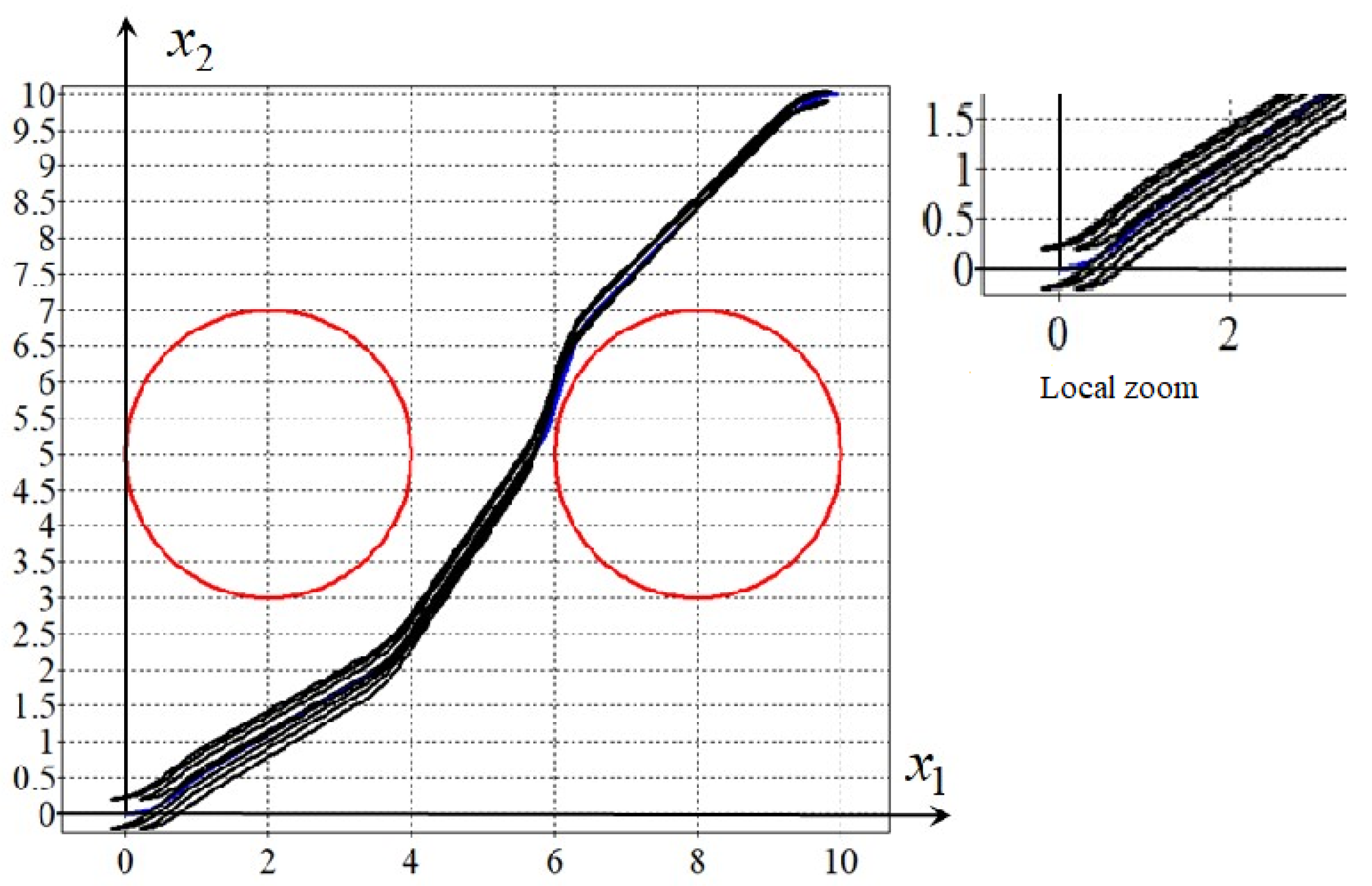
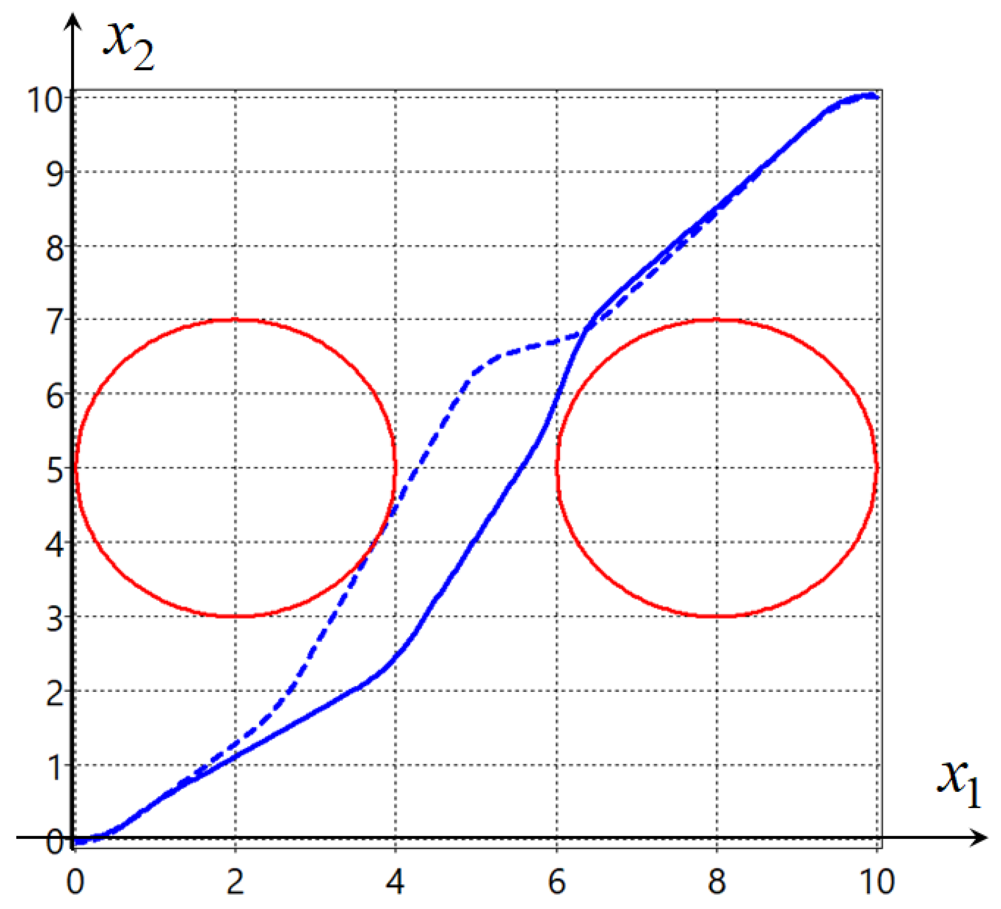
Figure 5 shows the trajectories of two robots with the control system (58) from some initial states. None of the trajectories violate the phase constraints and they almost reach terminal states. The average value of the quality criterion (52) was $J_4=2.21$.

If we solved the optimal control problem in the classical statement and then synthesised the control system for motion stabilisation along the optimal trajectory, then the control synthesis problem for motion stabilisation took too much time.

4.3. Stabilisation System Synthesis

It was proposed to first solve the synthesis problem of the universal stabilisation system. Universal means that the stabilisation system stabilises the motion along a class of trajectories. Then, the optimal control problem is solved in a class of optimal trajectories that can be stabilised using an already obtained stabilisation system of motion along the trajectory.

We considered the synthesis problem of the universal stabilisation system for motion along the given trajectories. For this purpose, we created one stabilisation system for one robot to work in tandem with the two optimal trajectories, obtained upon solving the optimal control problem and starting from two different initial states.

In the stabilisation synthesis problem, the mathematical model of one robot is considered as follows:

$$\begin{array}{ccc}\hfill {\dot{x}}_1& =& 0.5(u_1+u_2)cos\left(x_3\right),\hfill \\ \hfill {\dot{x}}_2& =& 0.5(u_1+u_2)sin\left(x_3\right),\hfill \\ \hfill {\dot{x}}_3& =& 0.5(u_1-u_2).\hfill \end{array}$$

(63)

Control constraints are given as follows:

$$-10=u^{-}⩽u_i⩽u^{+}=10,i=1,2.$$

(64)

Two sets of initial states are given as follows:

$$\begin{array}{ccc}\hfill {\mathrm{X}}_{0,1}& =& \{{\mathbf{x}}^{0,1,1},\dots ,{\mathbf{x}}^{0,1,K}\},\hfill \\ \hfill {\mathrm{X}}_{0,2}& =& \{{\mathbf{x}}^{0,2,1},\dots ,{\mathbf{x}}^{0,2,K}\},\hfill \end{array}$$

(65)

where

$${\mathbf{x}}^{0,j,i}={\mathbf{x}}^{0,j}-{\Delta }_0+{(i-1)}_2\odot 2{\Delta }_0,j=1,2,$$

(66)

${\mathbf{x}}^{0,1}$ and ${\mathbf{x}}^{0,2}$ are the initial states of each robot (29), ${\Delta }_0={[0.20.2\pi /18]}^T$, and ${(i-1)}_2$ is a three-bit binary code of $i-1$ number, $i=1,\dots ,2^3=8$.

Two program trajectories are given as follows:

$${\mathbf{x}}^{*,1}\left(t\right),{\mathbf{x}}^{*,2}\left(t\right),$$

(67)

which are particular solutions of the reference model:

$$\begin{array}{ccc}\hfill {\dot{x}}_1^{*}& =& 0.5(u_1^{*}+u_2^{*})cos\left(x_3^{*}\right),\hfill \\ \hfill {\dot{x}}_2^{*}& =& 0.5(u_1^{*}+u_2^{*})sin\left(x_3^{*}\right),\hfill \\ \hfill {\dot{x}}_3^{*}& =& 0.5(u_1^{*}-u_2^{*}),\hfill \end{array}$$

(68)

from the initial states (29) with the program control in the form of a piece-wise linear function

$$u_i^{*,j}=\left\{\begin{array}{c}{u}^{+},\mathrm{if}{u}_i^{+}⩽v_i^{*,j}\left(t\right)\hfill \\ u^{-},\mathrm{if}{v}_i^{*,j}\left(t\right)⩽u^{-}\hfill \\ v_i^{*,j},\mathrm{otherwise}\hfill \end{array}\right.,j=1,2,i=1,2,$$

(69)

where

$$v_i^{*,j}=\left({\tilde{q}}_{i+(k-1)m}^{\left(j\right)}\right)+({\tilde{q}}_{i+km}^{\left(j\right)}-{\tilde{q}}_{i+(k-1)m}^{\left(j\right)}){\displaystyle \frac{t-(k-1)\Delta t}{\Delta t}},(k-1)\Delta t⩽t<k\Delta t,$$

(70)

$k=1,\dots ,L$, ${\tilde{\mathbf{q}}}^j={[{\tilde{q}}_1^{\left(j\right)}\dots {\tilde{q}}_{(k+1)m}^{\left(j\right)}]}^T$, j is the trajectory number, $j=1,2$,

$$\begin{array}{ccc}\hfill {\tilde{\mathbf{q}}}^1& =& [16.79762-4.891742.556025.6187215.76362\hfill \\ \hfill & & 17.2623214.749831.2650414.9553119.27486\hfill \\ \hfill & & 18.021043.140180.7218218.0360818.22479\hfill \\ \hfill & & {16.7853411.5681910.32455-19.4088914.18273]}^T,\hfill \\ \hfill {\tilde{\mathbf{q}}}^2& =& [16.96601-9.2092914.652698.5726919.99868\hfill \\ \hfill & & 16.33206-1.2407219.8176619.99986-6.24985\hfill \\ \hfill & & 15.8862719.9449716.3447618.280703.31875\hfill \\ \hfill & & {17.0317911.1949416.76657-5.2885817.98243]}^T.\hfill \end{array}$$

(71)

Both program trajectories have the last points in the terminal states of

$$\begin{array}{ccc}\hfill {\mathbf{x}}^{*,1}\left(t_f\right)& =& {\mathbf{x}}^{f,1}={\left[10100\right]}^T,\hfill \\ \hfill {\mathbf{x}}^{*,2}\left(t_f\right)& =& {\mathbf{x}}^{f,2}={\left[00\pi \right]}^T.\hfill \end{array}$$

(72)

It necessary to find a control function in the form of

$$\mathbf{u}=\mathbf{h}({\mathbf{x}}^{*,j}-\mathbf{x}),j=1,2,$$

(73)

where j is the program trajectory number.

The quality criterion is given as follows:

$$J_5=\sum _{j=1}^2\sum _{k=1}^K\left(p_1\parallel {\mathbf{x}}^{f,j}-x(t_{f,k},{\mathbf{x}}^{0,k})\parallel +\underset{0}{\overset{t_{f,k}}{\int }}\parallel {\mathbf{x}}^{*,j}\left(t\right)-\mathbf{x}(t,{\mathbf{x}}^{0,k})\parallel dt\right)\to \underset{\mathbf{h}({\mathbf{x}}^{*,j}-\mathbf{x})}{min}.$$

(74)

To solve the control synthesis problem, machine learning control via the network operator method was used. The network operator method was performed with the following parameters: an NOP matrix size of $24\times 24$, six source nodes for the NOP graph, including three nodes for variables and three nodes for searched parameters, and two sink nodes for the output components of the control vector. The variational genetic algorithm parameters were as follows: the number of possible solutions in initial population—512; the number of crossover operations in one generation—128; the number of generations—128; the depth of variation—7; the number of generations between change in the basic solution—20; the number of bits for coding a parameter—16.

The following solution was obtained:

$$h_i({\mathbf{x}}^{*}-\mathbf{x})=\left\{\begin{array}{c}{u}^{+},\mathrm{if}{u}^{+}⩽{\tilde{h}}_i({\mathbf{x}}^{*}-\mathbf{x})\hfill \\ u^{-},\mathrm{if}{\tilde{h}}_i({\mathbf{x}}^{*}-\mathbf{x})⩽u^{-}\hfill \\ {\tilde{h}}_i({\mathbf{x}}^{*}-\mathbf{x}),\mathrm{otherwise}\hfill \end{array}\right.,$$

(75)

where

$$\begin{array}{l}{\tilde{h}}_1({\mathbf{x}}^{*}-\mathbf{x})=\mu \left(W\right)+H+{\rho }_2(exp\left(G\right))+{\rho }_3\left(D\right)+{\rho }_3\left(B\right)+C^2+\\ exp\left(B\right)+\vartheta \left(q_2(x_2^{*}-x_2)\mathrm{sgn}(x_1^{*}-x_1)\right)+{(x_3^{*}-x_3)}^2-(x_2^{*}-x_2),\end{array}$$

(76)

$${\tilde{h}}_2({\mathbf{x}}^{*}-\mathbf{x})={\tilde{h}}_1({\mathbf{x}}^{*}-\mathbf{x})+\mathrm{sgn}\left(W\right)\sqrt{\left|W\right|}+{\rho }_2(exp\left(G\right))-F+ln\left(\right|G\left|\right)+{\left(q_3\right)}^{-1},$$

(77)

$$A=q_1(x_1^{*}-x_1)sin\left(q_1\right){(x_2^{*}-x_2)}^3,$$

$$B=q_3(x_3^{*}-x_3)exp\left(q_2\right)+q_2(x_2^{*}-x_2)\mathrm{sgn}(x_1^{*}-x_1),$$

$$C=A+\mu (x_3^{*}-x_3)+{(x_2^{*}-x_2)}^3+\mu (x_1^{*}-x_1),$$

$$D=B^2+C+\mathrm{sgn}\left(A\right)+{\rho }_2\left(q_3\right)+{\rho }_1(x_3^{*}-x_3)+\mathrm{sgn}(x_2^{*}-x_2)\sqrt{|x_2^{*}-x_2|},$$

$$E=D+{\left(q_3\right)}^{-1}+{\rho }_1(x_3^{*}-x_3),$$

$$F=B+exp\left(q_2(x_2^{*}-x_2)\mathrm{sgn}(x_1^{*}-x_1)\right)+{\rho }_3\left(q_1\right),$$

$$G={\rho }_1\left(E\right)+A^2+{\left(q_2(x_2^{*}-x_2)\mathrm{sgn}(x_1^{*}-x_1)\right)}^{-1}+tanh(x_3^{*}-x_3),$$

$$H=F+cos\left(F\right)+{\rho }_1\left(B\right)sin(q_3(x_3^{*}-x_3)exp\left(q_2\right))+arctan\left(q_2(x_2^{*}-x_2)\mathrm{sgn}(x_1^{*}-x_1)\right)+A-A^3,$$

$$W=H-H^3+E^2+\mathrm{sgn}\left(B\right)-B+ln\left(\right|q_3(x_3^{*}-x_3)exp\left(q_2\right)\left|\right)+cos(x_1^{*}-x_1),$$

$q_1=15.9375$, $q_2=1.29028$, $q_3=10.13403$. A network operator matrix is given in Appendix A. Here, the trajectory number is not indicated since it is assumed that the stabilisation system provides the control object motion along any given program trajectory from some class.

Figure 6 and Figure 7 show the perturbed trajectories from the first (Figure 6) and the second (Figure 7) given initial states.

If the obtained motion stabilisation system (75) was inserted into the mathematical models of the control objects (27), and the system was simulated without disturbances to the program trajectories obtained via the control (42) applied to the reference model (68). Then, the quality criterion for the optimal control problem was $J_3=2.088$, instead of $1.801$, which was obtained upon solving the origin optimal control problem. This result was expected, as the optimal control problem was solved for objects without a motion stabilisation system.

4.4. Optimal Control Problem with Advanced Control Object Model

Let us consider the same optimal control problem, but for the advanced mathematical model of the control object. There are two control objects described using the advanced mathematical model, including reference models for program trajectory generation.

$$\begin{array}{ccc}\hfill {\dot{x}}_1^{*,j}& =& 0.5(u_1^{(j)}+u_2^{(j)})cos(x_3^{*,j}),\hfill \\ \hfill {\dot{x}}_2^{*,j}& =& 0.5(u_1^{(j)}+u_2^{(j)})sin(x_3^{*,j}),\hfill \\ \hfill {\dot{x}}_3^{*,j}& =& 0.5(u_1^{(j)}-u_2^{(j)}),\hfill \\ \hfill {\dot{x}}_1^{(j)}& =& 0.5(h_1({\mathbf{x}}^{*,j}-{\mathbf{x}}^j)+h_2({\mathbf{x}}^{*,j}-{\mathbf{x}}^j))cos(x_3^{(j)}),\hfill \\ \hfill {\dot{x}}_2^{(j)}& =& 0.5(h_1({\mathbf{x}}^{*,j}-{\mathbf{x}}^j)+h_2({\mathbf{x}}^{*,j}-{\mathbf{x}}^j))sin(x_3^{(j)}),\hfill \\ \hfill {\dot{x}}_3^{(j)}& =& 0.5(h_1({\mathbf{x}}^{*,j}-{\mathbf{x}}^j)-h_2({\mathbf{x}}^{*,j}-{\mathbf{x}}^j)),\hfill \end{array}$$

(78)

where $j=1,2$.

A hybrid evolutionary algorithm was used. The previously found optimal solution (42) was included in the initial population as one of the possible solutions. This solution is the best in the initial population as other possible solutions are generated randomly, which makes it possible to not look for a completely new solution but to improve the previously found one for a problem with the advanced control object model.

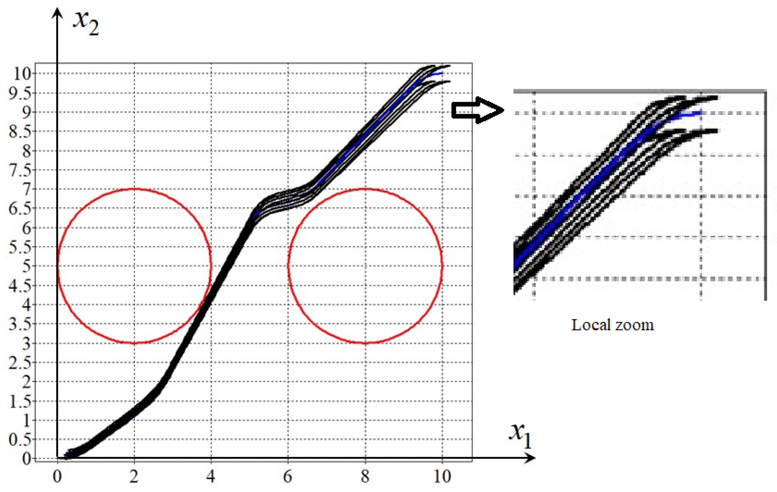
The following solution for the piece-wise linear approximation of the control function (38) was obtained:

$$\begin{array}{ccc}\hfill \tilde{\mathbf{q}}& =& [17.1163-5.197616.9293-8.88133.54706.893616.44418.8112\hfill \\ \hfill & & 16.918616.906919.042116.361815.26231.0616-0.691819.5165\hfill \\ \hfill & & 15.349818.020119.9420-6.102817.45614.808314.951620.0000\hfill \\ \hfill & & 0.897219.535515.997814.084519.982015.88312.415714.7072\hfill \\ \hfill & & {7.97917.605716.739015.9825-18.848510.4700-17.812815.6457]}^T.\hfill \end{array}$$

(79)

Figure 8 shows the optimal trajectories (79) for robots with the advanced mathematical model with a quality criterion value $J_3=1.937$. Optimal trajectories are marked with blue lines, and obstacles are marked with red circles.

5. Discussion

At present, obtaining the optimal control problem solution for multi-functional objects, such as robots in their functioning process, is highly desirable. This is even the case for an approximate solution that is fast and can be obtained on-board. Modern on-board processors allow us to solve problems in short periods of time, albeit in the classical statement, when the control function is searched for as a time function. It is well known and has been demonstrated in our computational experiments that such solutions obtained for original mathematical models are not feasible in practice as they lead to significant errors when the control object experiences small perturbations. The proposed approach of using the advanced method allows us to obtain optimal control problem solutions from the class of feasible control functions. The quality criterion includes penalties for violating both static and dynamic phase constraints. It should be noted that if the number and size of obstacles change, then the optimal control problem should be solved again for the same advanced model and another number of obstacles, and so on, and new optimal trajectories should be obtained, which will also belong to the class of trajectories that are stabilised via the trajectory motion stabilisation system.

The key factor in creating an advanced model is a set of control functions (7) that generate a class of trajectories (9). If the set (7) is sufficient, then the optimal control problem solution with the advanced model with a quality criterion value of (5) will be close to the optimal solution obtained solely for the reference model.

Creating an advanced model is always possible for tasks where the optimal control problem is stated for the model without uncertainties and stochastics in the right parts.

6. Conclusions

This study proposes using an advanced control object model. Initially, a universal motion stabilisation system along the specified trajectory is built for the object. It is assumed that, in the functioning process, the object will move along the optimal trajectories of a certain class. The resulting control system is then inserted into the control object. In order to quickly solve optimal control problems, an advanced object model is input into the on-board processor of the control object, which includes a mathematical model of the object with a motion stabilisation system along a given trajectory and a reference model that generates an optimal trajectory. While functioning, the evolutionary algorithm solves the optimal control problem in the classical statement in real time for an advanced control object model. The obtained solution is a control function for the reference model that generates a trajectory from a class of trajectories stabilised using the object control system.

7. Future Work

Further research will focus on developing effective methods for building advanced control object models, specifying the class of stabilisation trajectories and possibly the class of criteria for which these trajectories are optimal.