Enhancing Parameters Tuning of Overlay Models with Ridge Regression: Addressing Multicollinearity in High-Dimensional Data

Abstract

The extreme ultraviolet (EUV) photolithography process is a cornerstone of semiconductor manufacturing and operates under demanding precision standards realized via nanometer-level overlay (OVL) error modeling. This procedure allows the machine to anticipate and correct OVL errors before impacting the wafer, thereby facilitating near-optimal image exposure while simultaneously minimizing the overall OVL error. Such models are usually high dimensional and exhibit rigorous statistical phenomena such as collinearities that play a crucial role in the process of tuning their parameters. Ordinary least squares (OLS) is the most widely used method for parameters tuning of overlay models, but in most cases it fails to compensate for such phenomena. In this paper, we propose the usage of ridge regression, a widely known machine learning (ML) algorithm especially suitable for datasets that exhibit high multicollinearity. The proposed method was applied in perturbed data from a 300 mm wafer fab, and the results show reduced residuals when ridge regression is applied instead of OLS.

1. Introduction

According to Moore’s law, “the number of transistors that can be placed on a chip doubles every 24 months” [1]. Maintaining Moore’s law is highly challenging, because it calls for continuous advancement in a very complex industry. Despite this, recent developments in the production of integrated circuits (ICs), particularly in photolithography, have enabled the industry to keep up with the high process standards. Owing to its role in transferring a desired pattern to a photosensitive material on the wafer surface (photocurable material; most frequently, commercial photo resist [2]) by exposing it to ultraviolet (UV) or extreme-UV (EUV) light, photolithography [3] is a crucial component of the entire process. Wafers with a high overlay (OVL) and small critical dimension (CD) are the result of a successful photolithography process. The smaller the exposed pattern and the smaller the exposed ICs on the wafer, the better the OVL and the smaller the CD. Therefore, photolithography is the most crucial step in the production of integrated circuits comprising the base mechanism that supports Moore’s law.

In terms of hardware and software, photolithography machines rank among the most complex machines in the market. It is highly challenging to orchestrate and operate the machine in such a way that it satisfies the extremely stringent OVL and CD standards, given the machine’s more than 50 million lines of code and thousands of hardware modules. This precision is impossible for the hardware alone. Software control techniques that cope with hardware imperfections are essential components of the machine. Software will enable the machine to meet the OVL and CD KPIs, which will confirm the machine’s quality.

The fundamental premise underlying this is that the machine can precisely model anticipated wavefront aberrations at the nanoscale level. The software then adjusts the associated machine knobs, such as mirror locations, such that it compensates for the anticipated aberrations because it knows what to expect. The required pattern is then exposed to the fewest possible flaws because the predicted fingerprint is rectified before it reaches the wafer surface. Under these circumstances, we recognize that one of the most important and difficult responsibilities of the photolithography process is the ability to create precise models. These models are the primary tools for successful exposure.

The process of describing the spatial changes in the overlay (OVL) of the features being printed is known as OVL fingerprint estimation (FE) in photolithography. These discrepancies can be caused by several factors, including flaws in the mask or the lithography procedure itself. The OVL of the features at various positions on the wafer are often measured using specialized metrology instruments that can estimate fingerprints. Information regarding the spatial changes in the OVL is then extracted from the resulting data and utilized to generate a “fingerprint” of the lithography process. Modeling the OVL is an essential step in the FE process. OVL modeling is the process of creating mathematical and statistical models to forecast how various process parameters affect OVL. By modifying the lithography process parameters in real time to meet the necessary OVL criteria, these models can be used to improve the lithography process. To ensure a high yield and reliable performance of the lithography process, FE estimation is a crucial tool.

A polynomial model is a mathematical or statistical representation of a system or process and polynomial. The basis functions and parameters are the two main components of the model. The structure of the problem and the properties of the data being modeled influence the basis functions that are used. On the other hand, model parameters are the estimated values that are used to define the model and are derived from the data. The precise values of the basis functions that best suit the data are determined by the parameters. In our specific use case, we need to provide the model for OVL. A linear model for OVL is defined by

$$\begin{array}{c}\hfill m(x,y)=\mathsf{\Phi }\times p\end{array}$$

$\mathsf{\Phi }$ is the information matrix which consists of the basis function $\varphi (x,y)$, and p are the parameters of our model. The OVL polynomial has p coefficients or parameters. As described above, the information matrix $\mathsf{\Phi }$ is already known to us and, in that case, the goal of FE is to estimate the parameters p of our model.

Overlay control is a critical part that enables the exposure system to successfully imprint the complex patterns and meet the strict requirements of modern IC designs. The current photolithographic systems manage to successfully control overlay via a combination of advanced process control (APC) and metrology modules. Metrology contributes to defining and tuning the overlay models (so that they accurately describe the expected systematic and nonsystematic overlay errors [4,5,6]), as well as relating them to the corresponding controllable knobs of the exposure system [7]. The coupling of overlay error predictions, via overlay models, with machine knobs defines the so called run-to-run (R2R) paradigm of overlay control [8,9,10]. Obviously, for an R2R process to be successful, it is crucial that the overlay models can accurately estimate the expected overlay errors. Extensive research has been conducted in defining overlay models. In [11], multilevel state space models were defined based on existing physics models [12,13,14], where multilayer, stack up overlay error models were developed. Extensive research has been conducted for improving the overlay modeling process, with the focus being either on optimizing the wafer measurements ([15,16]) or on investigating different metrics and cost functions ([17] Zhang et al.).

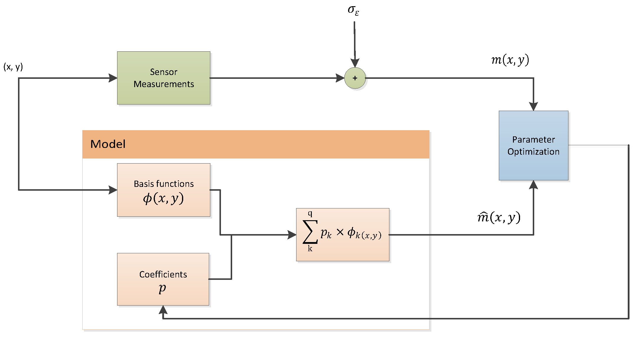
However, it is not sufficient to define the overlay model based only on the underlying physics; it is equally important that the metrology system further tunes the parameters of the overlay model. The ordinary least squares optimization (OLS) method is the most employed regression technique by the current exposure systems. OLS finds the regression coefficients of the overlay model that minimize the residual sum of the squared errors of the difference between the measured and the predicted overlay [18]. In Figure 1, the process of FE is presented. Since the basis functions of the model $\varphi (x,y)$ are already predefined, the goal of the FE process is to obtain the best estimation of the model parameters p.

Multicollinearity in high-dimensional datasets is a well-known challenge, particularly when multiple predictors are highly correlated. This can lead to unstable estimates in traditional regression models such as ordinary least squares (OLS), reducing their predictive power. To address this, alternative techniques such as principal component analysis (PCA), ridge regression, and lasso regression have been widely adopted. PCA is a dimensionality reduction technique that transforms the original variables into uncorrelated principal components, thereby eliminating multicollinearity by projecting the data into a lower-dimensional space where the principal components are orthogonal to each other [19]. Ridge regression adds an L2 regularization term to the OLS equation, which shrinks the coefficients of correlated variables, reducing their variance, and, thereby stabilizing the model [20,21]. Lasso regression, on the other hand, incorporates an L1 regularization term that not only shrinks the coefficients but can also set some of them exactly to zero, effectively performing variable selection while mitigating multicollinearity [22,23]. These methods are particularly useful when variable elimination is undesirable, as they allow the model to retain all the predictors while reducing the impact of multicollinearity on the predictive accuracy. Additionally, elastic net is an alternative approach particularly well suited for complex datasets. Elastic net combines both L1 (lasso) and L2 (ridge) penalties, making it highly effective in datasets that exhibit both multicollinearity and the need for variable selection. This hybrid approach balances the benefits of both ridge and lasso, allowing elastic net to handle correlated predictors and perform feature selection simultaneously [24]. When features in a dataset are highly correlated, the design matrix X in a linear regression model $Y=X\beta +ϵ$ becomes nearly singular or ill-conditioned. This condition leads to large variances in the least squares estimates of the coefficients, $\beta$, because the inverse of $X^{T}X$ (which is needed to compute the OLS estimates $\widehat{\beta }={\left(X^{T}X\right)}^{-1}{X}^{T}Y$) will be unstable or significantly influenced by small changes in X or Y. Ridge regression minimizes ${|Y-X\beta |}_2^2+\lambda {\left|\beta \right|}_2^2$, which shrinks coefficients smoothly and can handle collinearity better than lasso or PCA as it tends to reduce the coefficients proportionally, maintaining their relative influence on the outcome. Furthermore, ridge regression, by reducing the magnitude of all coefficients through its L2 penalty, tends to be more stable, although it does not reduce the model complexity by setting coefficients to zero.

A useful diagnostic tool to detect multicollinearity is the variance inflation factor (VIF), which quantifies how much the variance of a regression coefficient is inflated due to collinearity with other predictors. A high VIF value indicates that the parameter is highly collinear with others, making it problematic for reliable estimation. A general rule is that a VIF greater than 5 suggests moderate multicollinearity, while a VIF above 10 indicates a high level of multicollinearity [25]. By identifying variables that exhibit high variance inflation factor (VIF) values, we are able to determine which parameters induce multicollinearity. Subsequently, techniques such as principal component analysis (PCA), ridge, or lasso regression may be employed to address these issues, thereby enhancing the robustness of the model.

Importantly, the removal or combination of collinear parameters, while potentially reducing multicollinearity, is often undesirable because it can result in a significant loss of valuable information. Each predictor variable may carry unique and relevant aspects of the underlying data, and eliminating or combining them could obscure these nuances, leading to less precise and informative models [26]. Therefore, methods such as ridge or lasso regression, which allow for the retention of all variables while addressing the multicollinearity problem, are preferred in scenarios where preserving the integrity of the dataset is paramount.

In this paper, we are investigating the the fitness of the OLS algorithm for modeling highly dimensional overlay data. Among the aforementioned alternatives, we are proposing the usage of ridge regression over the classical OLS. The remainder of the paper is organized as follows: Section 2 describes the proposed method, and in Section 3 we show the results of applying the proposed method on an actual industrial process of 300 mm wafers. Finally, Section 4 presents the conclusions and potential future work.

2. Materials and Methods

In this paper, we propose to use ridge regression instead of the classic OLS method for tuning the parameters p of the overlay models. The overlay models, as mentioned above, consist of a set of basis functions $\varphi (x,y)$ that are already predefined based on the physics and specific parameters of the process. Ridge regression, or Tikhonov regularization [21], is a statistical method for estimating the parameters of multiple regression models in scenarios where the independent variables are highly correlated.

Ridge regression is particularly useful in ill-posed problems which exhibit multicollinearity in their independent variables. In our case, we try to find the vector p of parameters such that

$$\begin{array}{c}\hfill m=\mathsf{\Phi }\times p\end{array}$$

As mentioned before, the standard approach is to use the OLS method. OLS seeks to minimize the sum of the squared residuals:

$$\begin{array}{c}\hfill ||\mathsf{\Phi }p-{m\left|\right|}_2^2\end{array}$$

However, if no p satisfies the equation or more p do, then the problem is ill-posed and OLS might lead to an over- or underdetermined system of equations.

Ridge regression adds a regularization term ${\left|\right|\mathsf{\Gamma }x\left|\right|}_2^2$ for some suitable chosen matrix $\mathsf{\Gamma }=\alpha I$. This is known as $L_2$ regularization. This ensures smoothness and improves the conditioning of the problem. The minimization problem to be solved, then, is

$$\begin{array}{c}\hfill ||\mathsf{\Phi }p-{m\left|\right|}_2^2+{\left|\right|\mathsf{\Gamma }x\left|\right|}_2^2\end{array}$$

And the corresponding parameter vector p:

$$\begin{array}{c}\hfill p={({\mathsf{\Phi }}^T\mathsf{\Phi }+{\mathsf{\Gamma }}^T\mathsf{\Gamma })}^{-1}{\mathsf{\Phi }}^{T}m\end{array}$$

To select the regularization parameter, we employed the 10-fold cross-validation method. The 30 layers were used as the training dataset, while the remaining 10 layers served as the test set. The cross-validation process determined that the optimal regularization parameter was $\alpha =1.0$, which means that $\mathsf{\Gamma }=I$. A value of $\alpha =1.0$ means that the model benefits from a moderate amount of regularization, helping to stabilize the coefficient estimates and improve generalization without undermining the model’s ability to accurately capture the relationships between the features and the target variable. Essentially, the regularization helps prevent overfitting by reducing the influence of less important or highly correlated features, but it does not overpenalize the model to the point where its predictions become too simplistic or inaccurate.

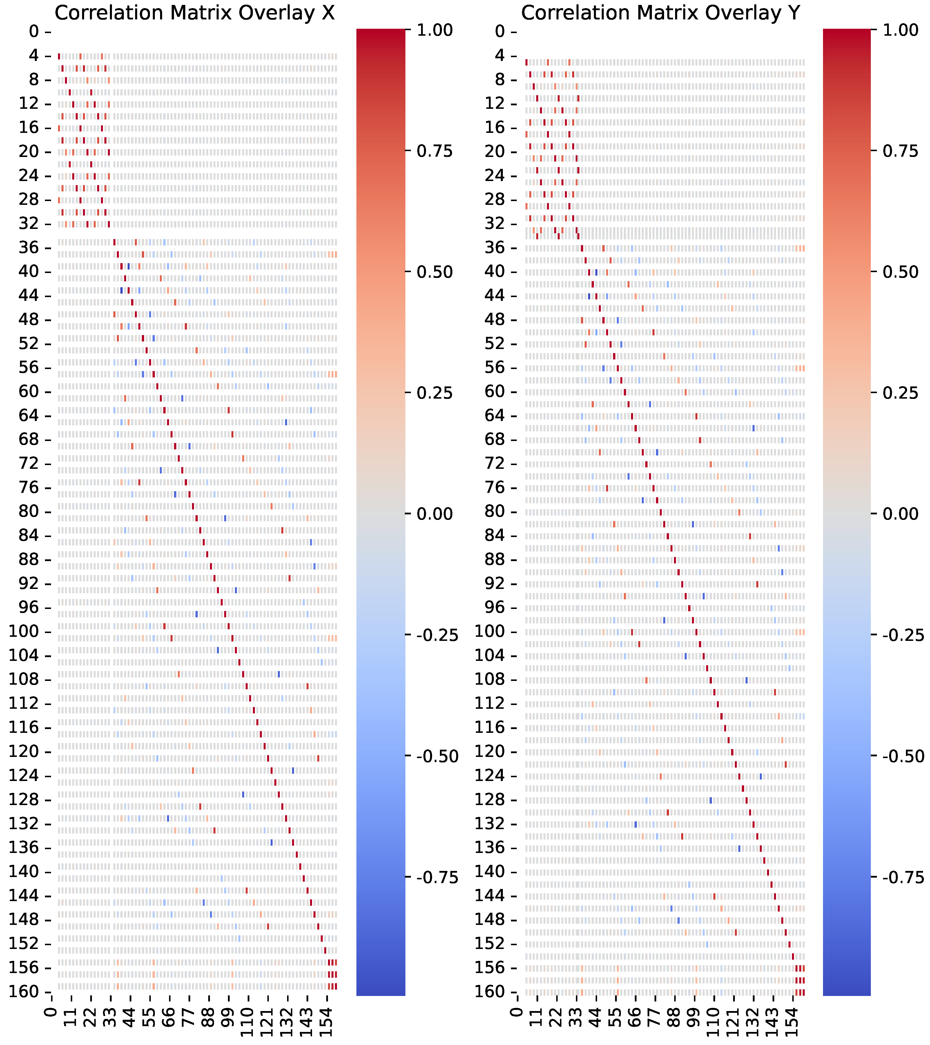
In Figure 2, the correlation matrix of the Overlay X and Overlay Y is presented. There seems to be high correlation between approximately 50 of the 161 parameters. This is an indication (a strong one, though) that there is significant collinearity in the parameters, and this needs to be further investigated.

The variance inflation factor $VIF$ is a statistical measure that quantifies the degree of multicollinearity for each independent variable. $VIF$ is calculated as follows:

$$\begin{array}{c}\hfill VIF=1/(1-R^2)\end{array}$$

with $R^2$ being the square of the OLS solutions. A value of $VIF>5$ indicates moderate multicollinearity, while $VIF>10$ indicates high multicollinearity. Performing the $VIF$ check in our OLS solutions for Overlay X and Y results in high mulitcollinearity in 62/161 parameters for Overlay X and in 109/161 parameters for Overlay Y. Therefore, the conclusion is that multicollinearity needs to be addressed. In this case, indeed, the ridge regression method should be able to address the issue and improve the parameter estimation method.

3. Results and Discussion

In our experiments, we compared the overlay residuals (in X and in Y) for both ridge regression and OLS methods. The expected overlay, per field point, is compared to the actual overlay. Next, a statistical analysis of the results is performed. In assessing the performance we use the $99.7$th percentile and $max$ residual metrics. Utilizing these metrics enables a comprehensive understanding of the overlay performance, providing insights into the extent of variability and the upper bounds of error dispersion.

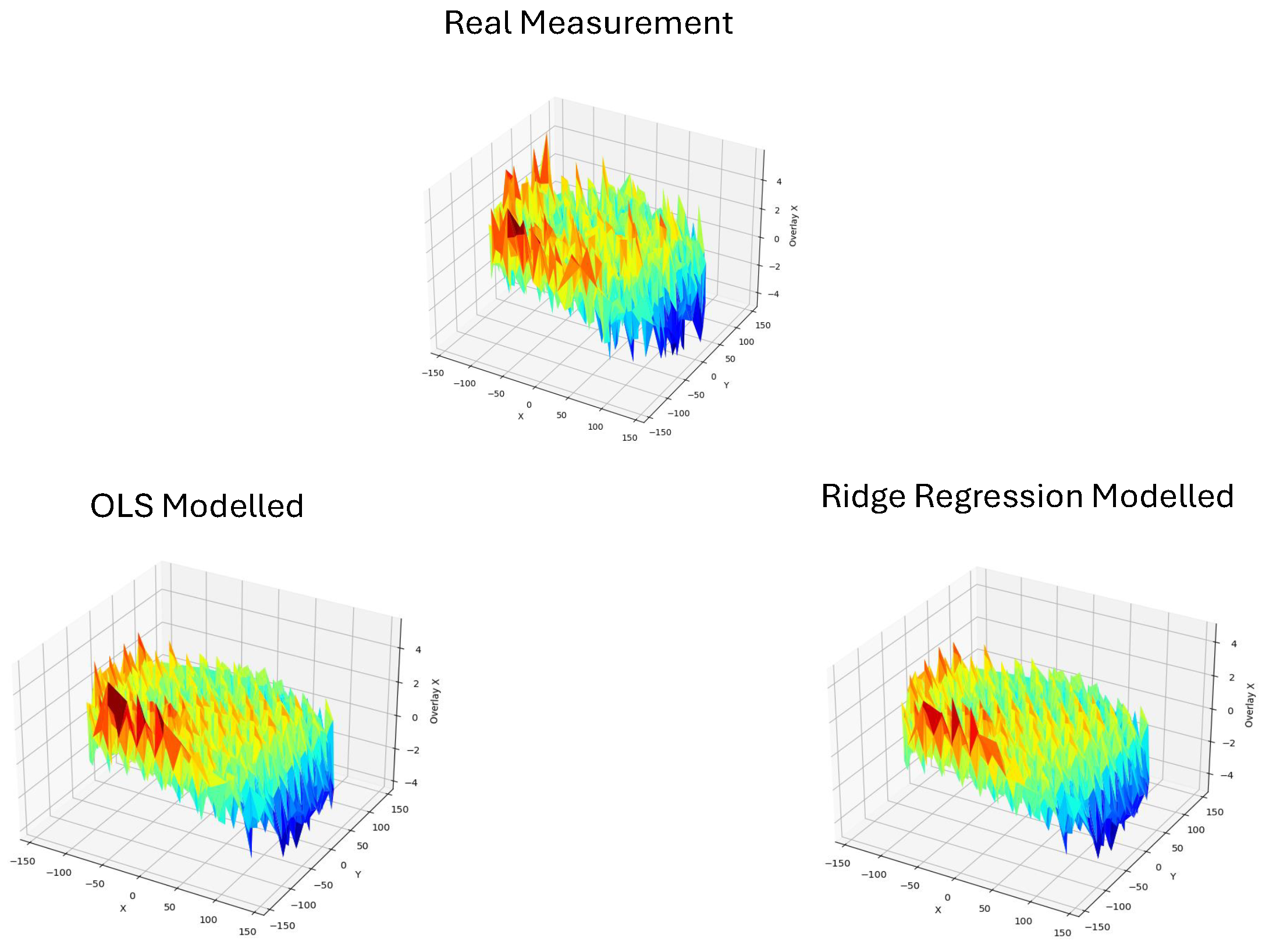
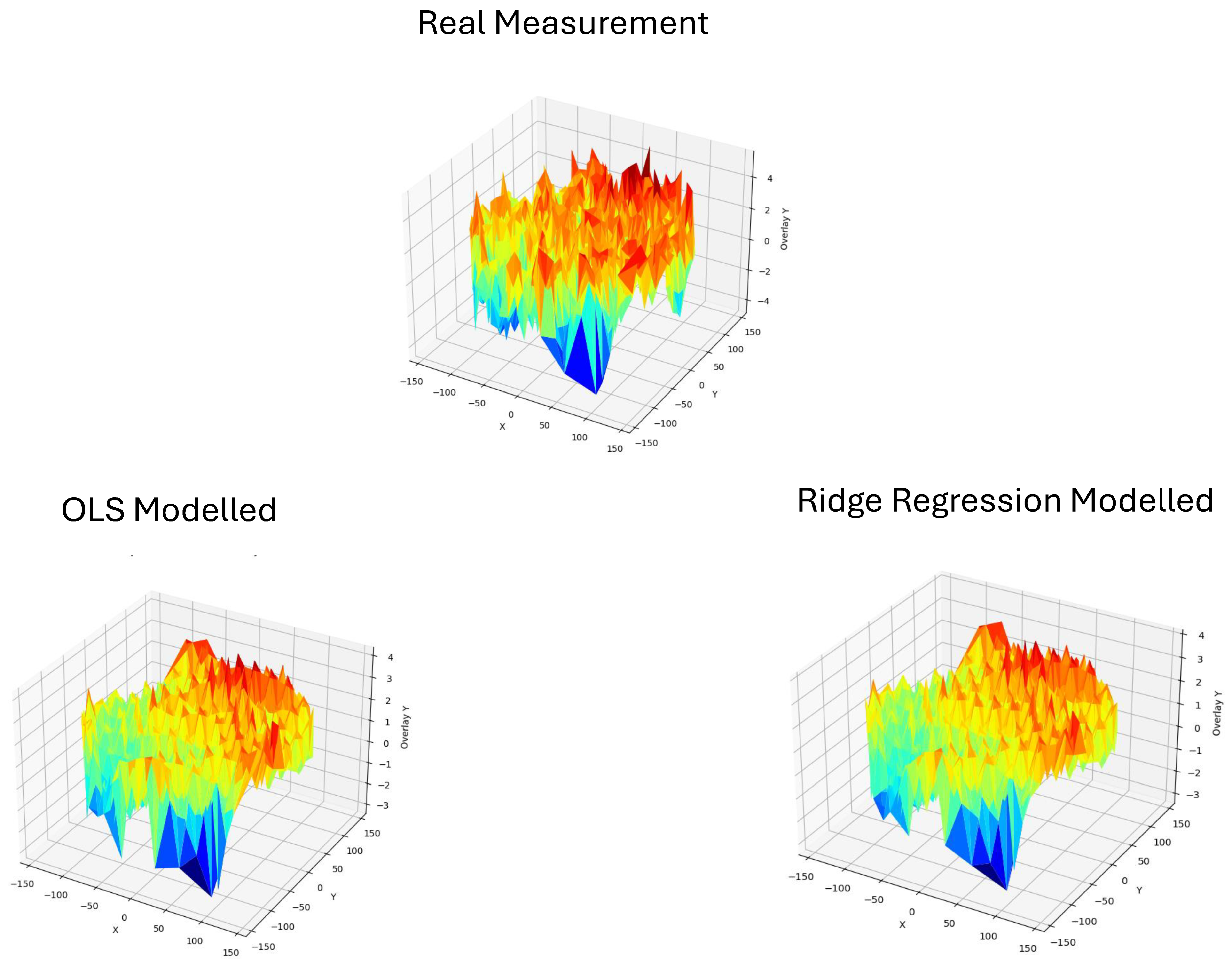
The goal of our method is to accurately model the measured overlay and reproduce it with minimum error. In Figure 3, we can see the measured Overlay X on the left and the modeled Overlay X on the right, using the ridge regression method. In this visual representation, we can see that the modeled overlay is able to successfully capture the expected overlay. Also, in areas of the wafer where there seems to be abnormal behavior as on the edges of the wafer, the patterns seems to really match. Similarly, in Figure 4, ridge regression also performs well on Overlay Y.

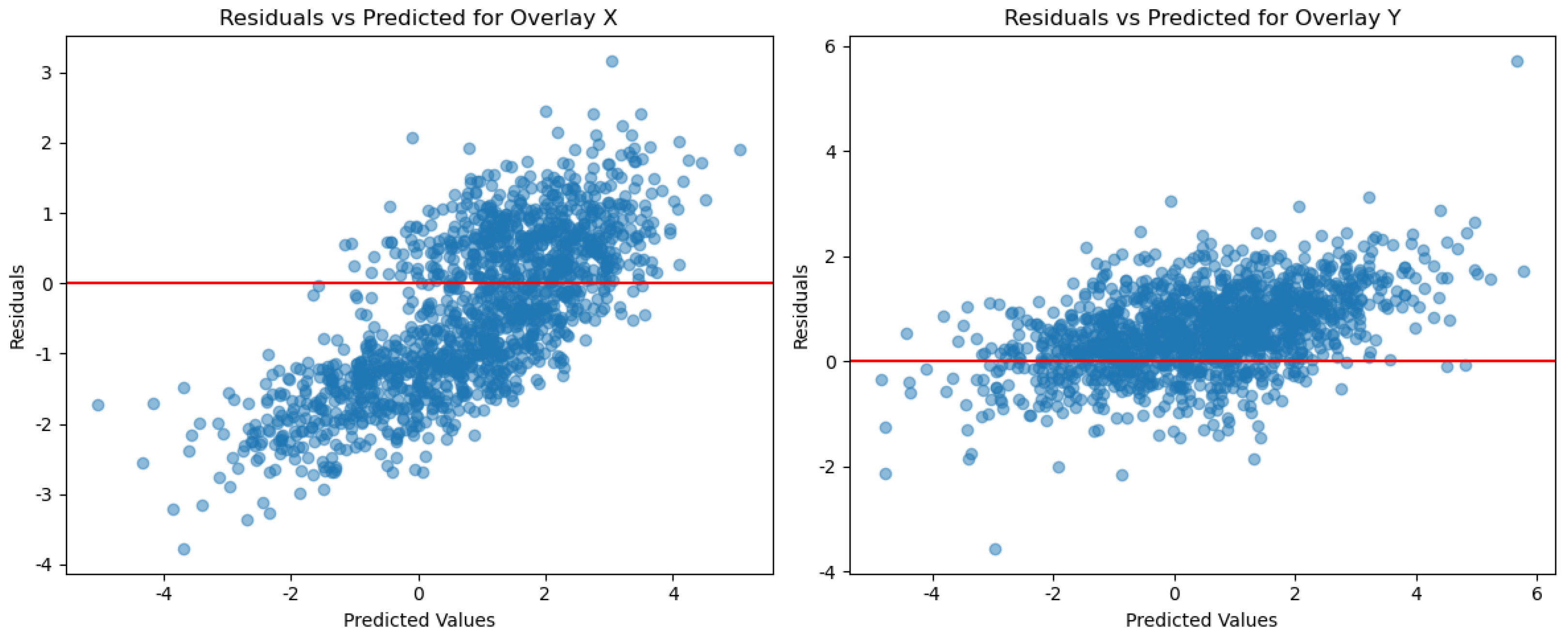
The residuals vs. the predicted values for ridge regression and OLS are presented in Figure 5 and Figure 6, respectively.

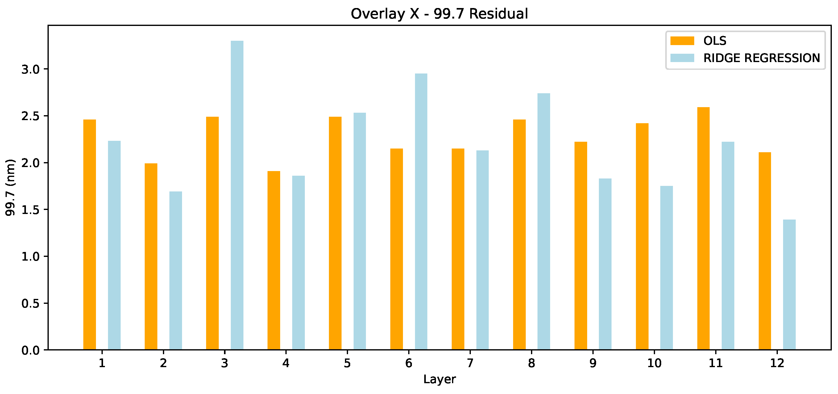
In Figure 7, the Overlay X residuals in 99.7 are presented for both OLS and ridge regression methods. For 8/12 layers, ridge regression outperforms the OLS method. Despite the overall model exhibiting certain statistical properties, such as multicollinearity, it is important to recognize that each layer in the process can behave differently. Several factors, particularly measurement noise, can significantly impact individual layers. In our case, this measurement noise plays a substantial role in the variability of the process. As a result, it is not surprising that OLS may outperform ridge regression in specific layers, such as layers 3, 5, and 6, where the unique characteristics of the exposure process may not benefit as much from regularization. In these cases, OLS may capitalize on the direct relationships between variables without the need for regularization, whereas ridge regression’s penalty on coefficients may dampen the model’s performance. However, it is important to focus on the overall performance of the model, rather than isolated instances. The broader trends across all layers indicate that ridge regression remains a robust choice, particularly in mitigating the effects of multicollinearity, even if OLS is favored in specific layers due to the unique “exposure specifics” that tend to influence the outcome.

The max residuals in Overlay X are compared in Figure 8. Here, we observe a different pattern than in 99.7. OLS outperforms the ridge regression in 9/12 layers. From these results, we cannot yet draw a safe conclusion. It depends which metric we value most (99.7 vs. max), and this actually depends on the use case. However, the superiority of ridge regression in 99.7 only is an interesting conclusion already.

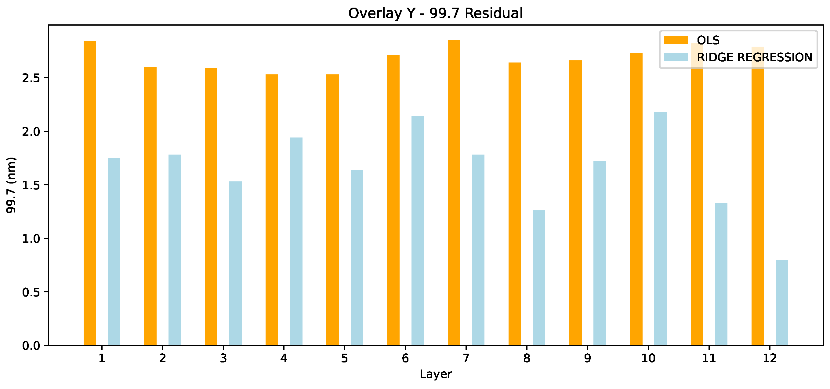
When checking the Overlay in Y, we draw a more clear picture of the situation. As presented in Figure 9, ridge regression significantly outperforms the OLS in all 12 layers. On average, this is a 1.04 nm improvement. In this case, the superiority of ridge regression is clear.

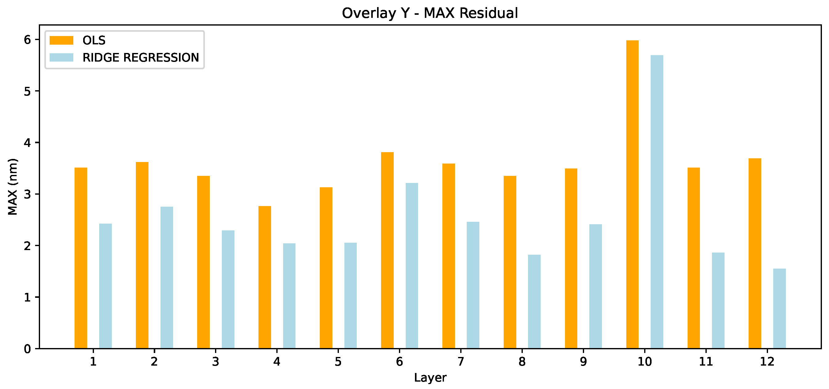
Similarly, in Overlay max, Figure 10 shows ridge regression outperforming OLS in all wafers with an average improvement of 1.10 nm.

The results presented in

Table 1. Overlay X residuals in nanometers.

Layer	OLS—99.7	Ridge—99.7	OLS—Max	Ridge—Max
1	2.46	2.23	3.03	3.88
2	1.99	1.69	5.14	4.65
3	2.49	3.3	3.27	4.71
4	1.91	1.86	2.96	3.09
5	2.49	2.53	3.51	3.7
6	2.15	2.95	2.58	4.09
7	2.15	2.13	2.72	3.17
8	2.46	2.74	3.31	4.08
9	2.22	1.83	2.88	2.96
10	2.42	1.75	3.54	2.98
11	2.59	2.22	4.01	4.28
12	2.11	1.39	2.81	2.12

and

Table 2. Overlay Y residuals in nanometers.

Layer	OLS—99.7	Ridge—99.7	OLS—Max	Ridge—Max
1	2.84	1.75	3.51	2.42
2	2.60	1.78	3.62	2.75
3	2.59	1.53	3.35	2.29
4	2.53	1.94	2.76	2.04
5	2.53	1.64	3.13	2.05
6	2.71	2.14	3.81	3.21
7	2.85	1.78	3.59	2.46
8	2.64	1.26	3.35	1.82
9	2.66	1.72	3.49	2.41
10	2.73	2.18	5.98	5.69
11	2.82	1.33	3.51	1.86
12	2.79	0.80	3.69	1.55

illustrate the performance of ridge regression compared to ordinary least squares (OLS) across multiple layers in terms of the OVL X and OVL Y metrics, both for the $99.7$th percentile residuals and the maximum residuals. In Table 1, which focuses on OVL X, ridge regression generally performs better than OLS, particularly in reducing the $99.7$th percentile residuals. This is evident in most layers where the ridge regression residuals are consistently lower than those obtained using OLS. For instance, in layer 9, ridge regression produces a $99.7$th percentile residual of 1.83 nm compared to 2.22 nm with OLS. Similarly, the max residuals also show improvement in many cases, such as in layer 8, where ridge regression results in a max residual of 4.08 nm compared to 3.31 nm for OLS. On average we can also see that Ridge Regression achieves smaller residuals in 99.7, however on MAX it performs worse than OLS on average. 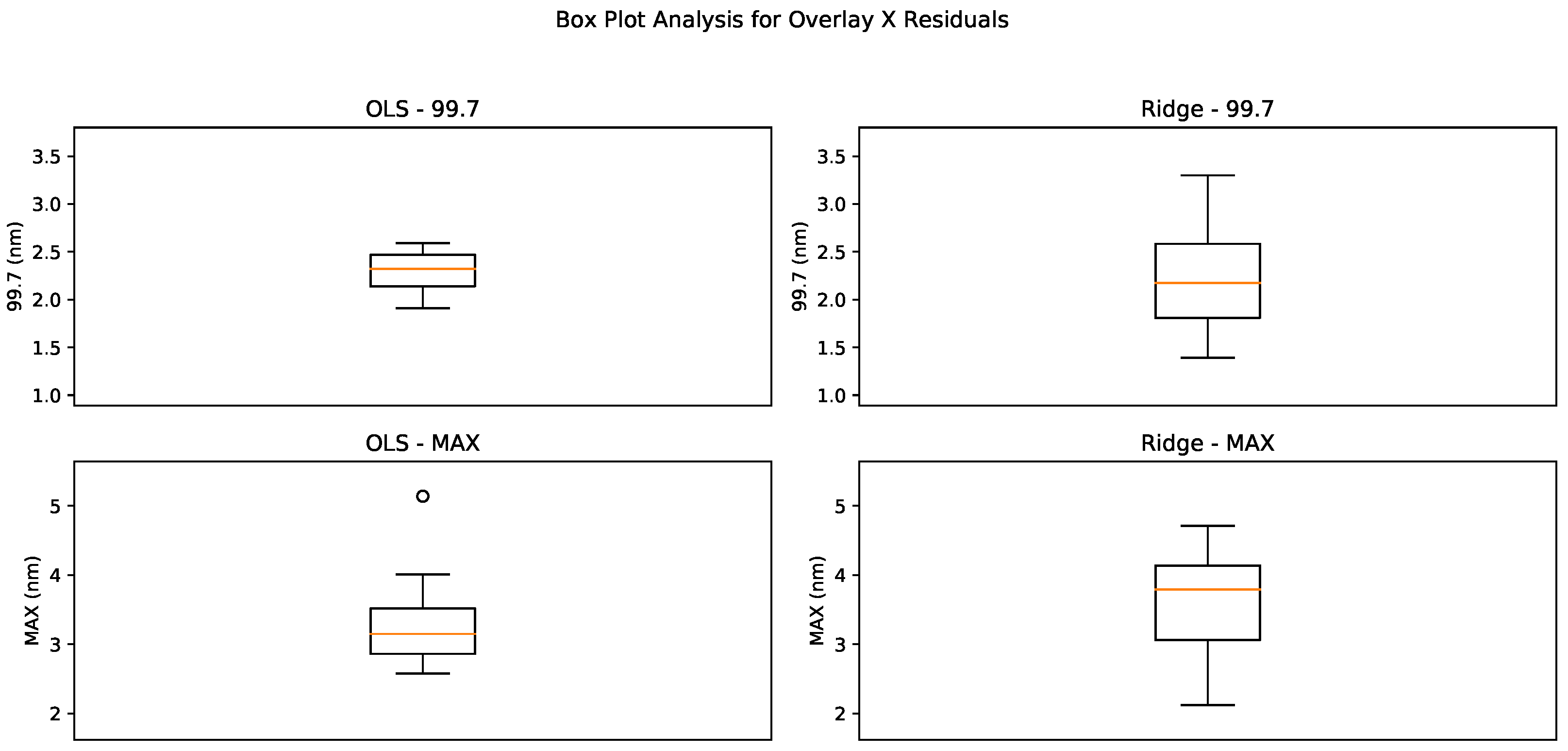In Figure 11 we see the box plots for the Overlay X. For the metric 99.7, the OLS residuals exhibit a tight Interquartile Range (IQR) centered approximately around 2.4 nm, indicating a generally consistent performance across different samples. The Ridge residuals, while similar in median value, show a slightly wider IQR with values stretching from about 1.7 nm to nearly 2.7 nm. This suggests that while the Ridge model can occasionally offer a tighter fit, it might also produce more variable results in some instances. For the MAX residuals, both models demonstrate an increase in the spread of values compared to the 99.7 measurements. The OLS model displays an IQR from approximately 3.0 nm to 3.5 nm, with some outliers extending towards 4.0 nm, indicating a less consistent fit for maximum residual values. The Ridge model, while showing a lower starting point at around 2.0 nm, extends up to about 4.5 nm, matching the OLS model in variability. The presence of outliers in both models for the MAX residuals suggests that extreme values are a common occurrence, potentially indicating challenging scenarios where both models struggle to maintain a consistent performance.

In Table 2, which reports the Overlay Y residuals, ridge regression again shows superior performance over OLS. This is particularly noticeable in the max residuals, where ridge regression substantially outperforms OLS in most layers. For example, in layer 10, the OLS max residual is 5.98 nm, while ridge regression achieves a significantly lower value of 5.69 nm. The same trend is visible in the $99.7$th percentile residuals, where ridge regression consistently yields lower residuals, such as in layer 3, where the residuals drop from 2.59 nm with OLS to 1.53 nm with ridge regression. 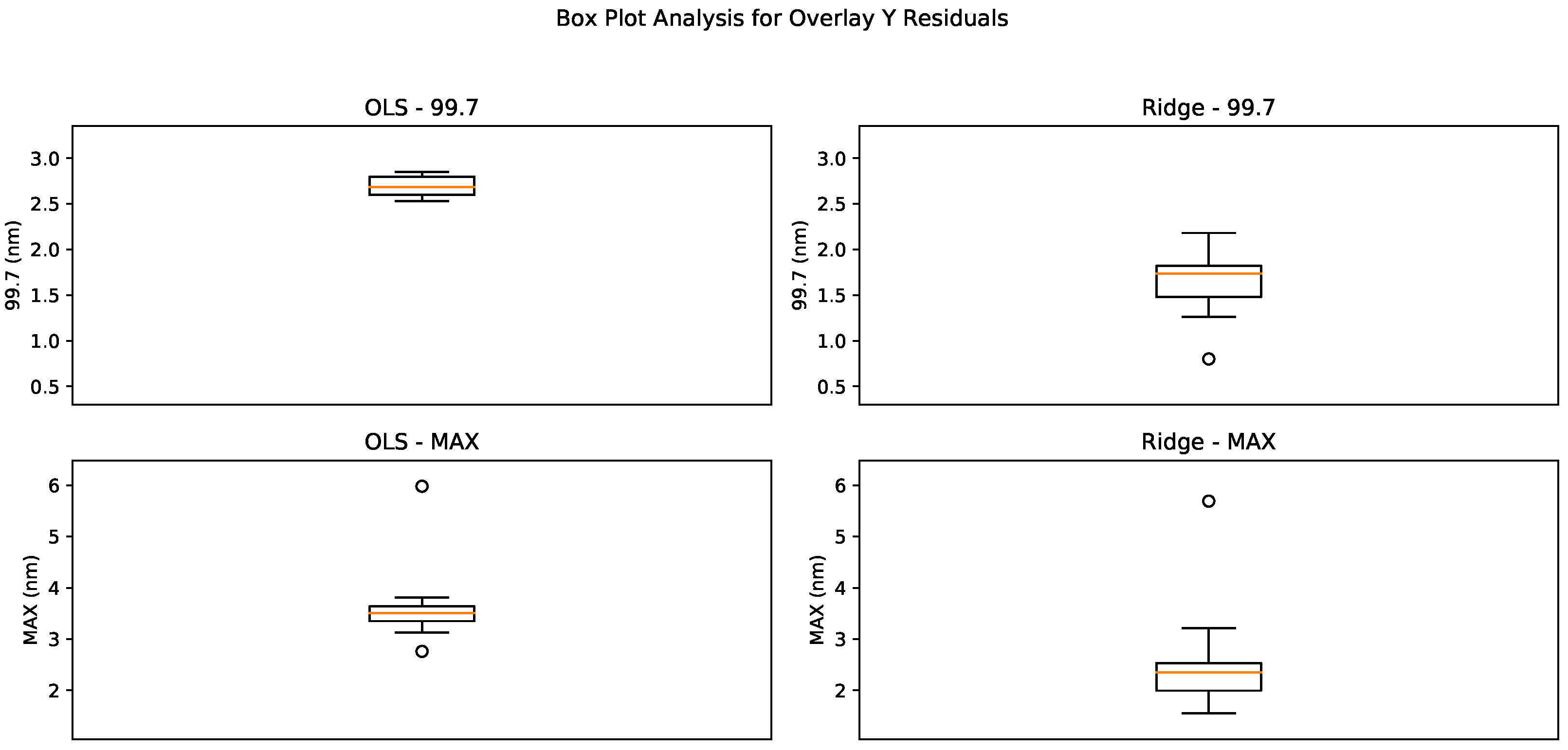In Figure 12 we see the box plots for Overlay Y. For the 99.7 metric, the OLS model exhibits a compact distribution with an IQR closely centered around 2.6 nm to 2.8 nm. This suggests a relatively stable and consistent model performance over the observed dataset. Ridge model demonstrates a significantly wider IQR, extending from 1.5 nm to 2.0 nm. The wider spread and lower minimum values may indicate a greater variability in model performance, potentially offering lower residuals but with less consistency compared to the OLS model. In the MAX nm residuals, the OLS residuals span from approximately 3.5 nm to 3.8 nm. Ridge residuals are slightly more spread ranging from 2 nm to approximately 2.8 nm.

Overall, the results clearly demonstrate that ridge regression provides better accuracy and robustness in reducing both $99.7$th percentile and max residuals compared to OLS. This improvement is particularly beneficial in handling multicollinearity within the dataset, a well-known strength of ridge regression. The reduced variance in the ridge regression models contributes to more reliable and consistent predictions across all layers, making it the preferred method in this context.

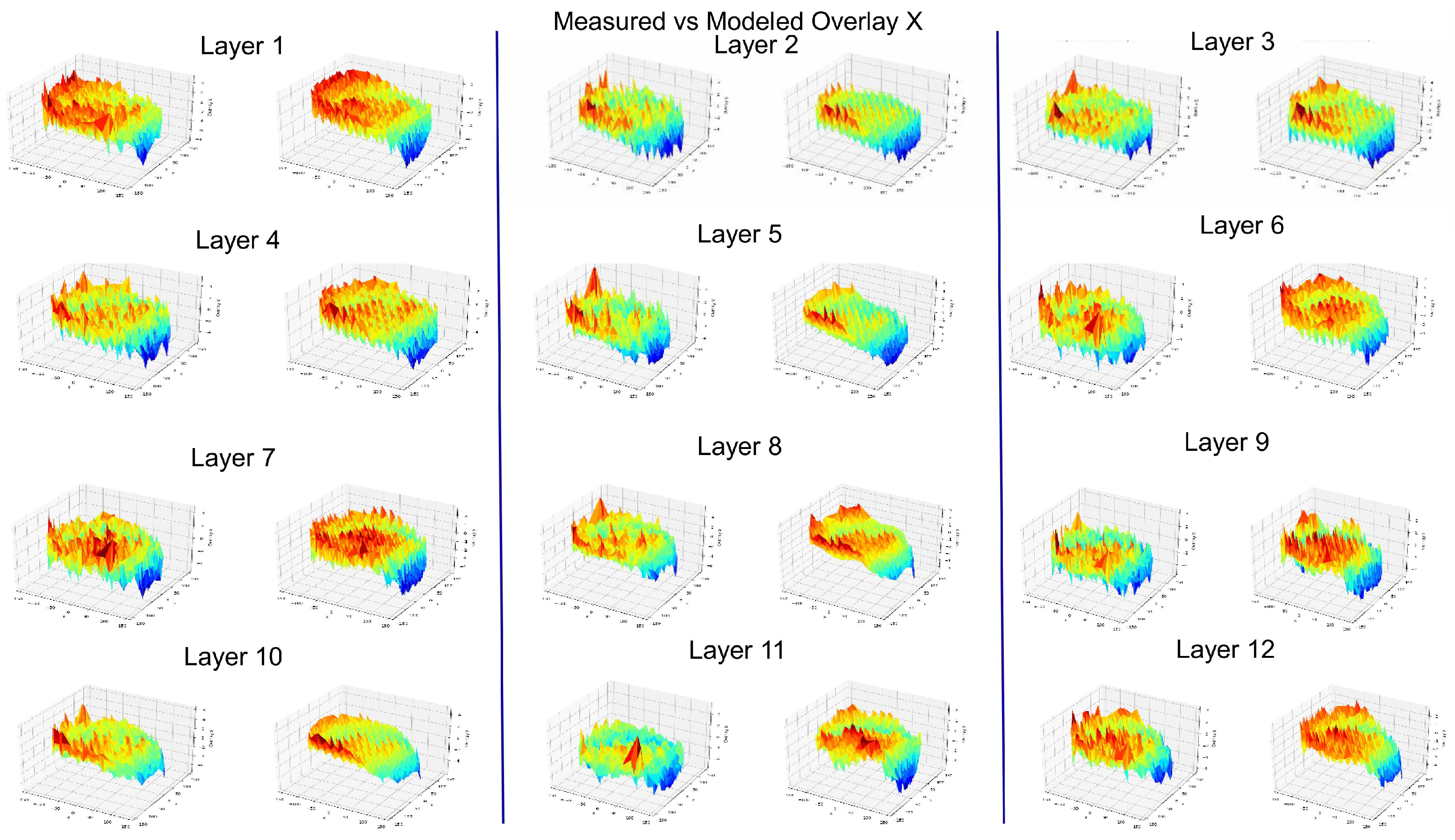
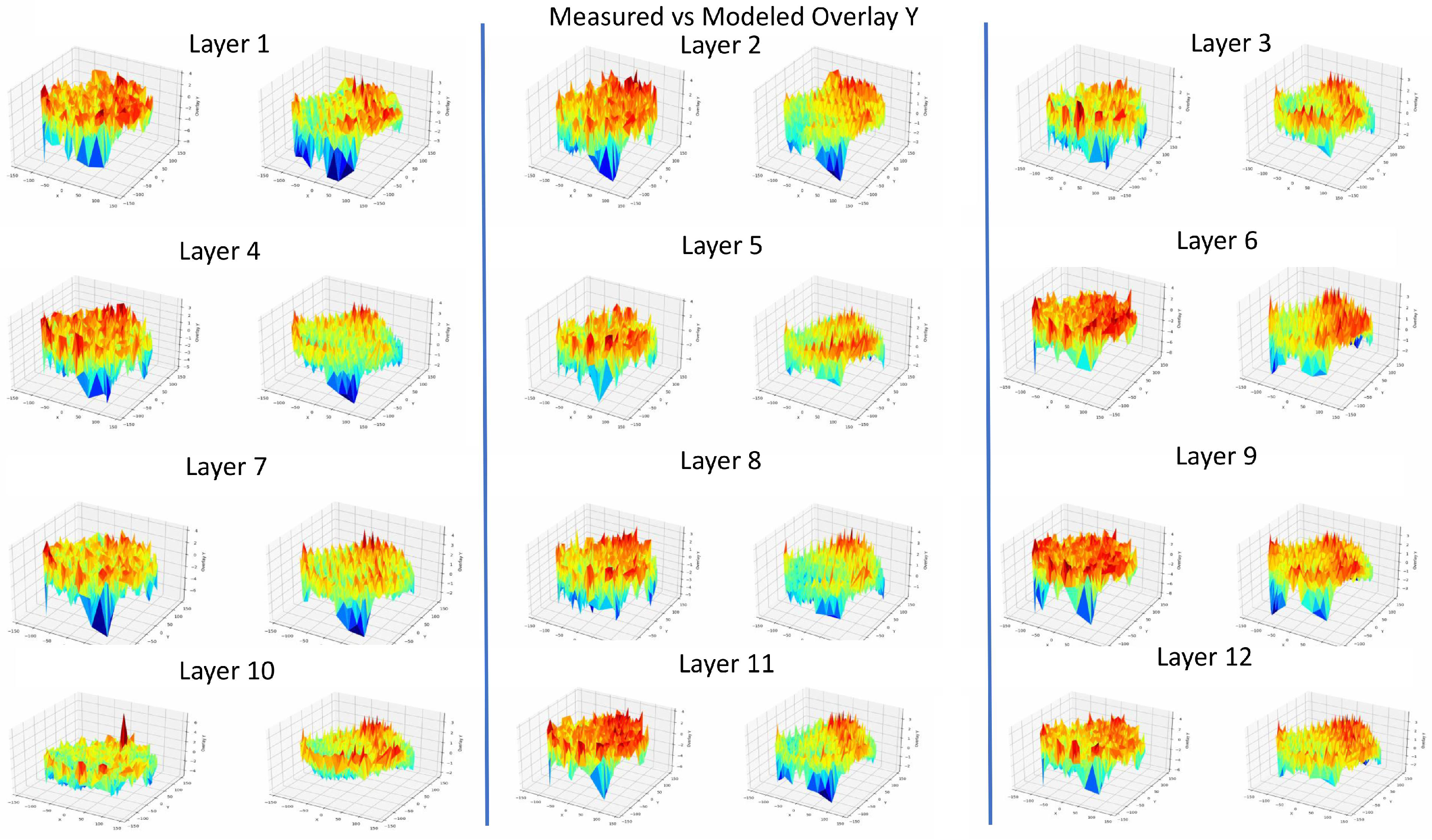
In Figure 13 and Figure 14, we present the measured vs. modeled Overlay X and Y for all the 12 layers. The observed differences between the measured and modeled results can be attributed to several factors. First, despite the application of ridge regression to address multicollinearity, the strong collinearity between certain parameters may still impact the model’s accuracy in specific cases, leading to discrepancies. Additionally, boundary effects at the edges of the wafer, where the photolithography process is more susceptible to physical limitations, may result in larger residuals, as these regions are often harder to model accurately. Moreover, while the polynomial model employed in this study is effective for many cases, it may not fully capture all the nonlinearities and complex interactions inherent in the photolithography process, particularly for edge cases. Lastly, measurement noise or inaccuracies in the metrology system may also contribute to the differences observed, as these errors can introduce additional variability that the model cannot entirely account for. Addressing these discrepancies may require further refinement of the model or adjustments to the regularization parameters used in the ridge regression approach. However, despite these discrepancies, the overall modeling performance remains satisfactory, as depicted by the residuals, which consistently show a good fit between the measured and modeled data across the majority of layers and regions. This indicates that the ridge regression approach still provides robust results in the context of overlay modeling.

4. Conclusions and Future Work

Ridge regression results indicate an obvious superiority over OLS when the data exhibit multicollinearity. Especially in Overlay X, where this phenomenon is more intense, ridge regression outperforms OLS in every single layer. In the end, the overall improvement in 99.7 is 1.04 nm and in the max 1.10 nm. Such a performance improvement at the sub-nanometer level of precision cannot be ignored. It is clear that OLS needs to be enhanced for similar datasets. One potential direction for future work would be the investigation of improving the model itself, either by reducing the features or by dynamically, during wafer production, selecting the most informative ones depending on the state of the process.