Article

From the DeGroot Model to the DeGroot-Non-Consensus Model: The Jump States and the Frozen Fragment States

1
College of Media Engineering, Communication University of Zhejiang, Hangzhou 310018, China
2
College of Physics and Electronic Engineering, Sichuan Normal University, Chengdu 610101, China
3
School of Science, Beijing University of Posts and Telecommunications, Beijing 100876, China
*
Author to whom correspondence should be addressed.
Mathematics 2024, 12(2), 228; https://doi.org/10.3390/math12020228
Submission received: 14 November 2023 / Revised: 12 December 2023 / Accepted: 15 December 2023 / Published: 10 January 2024
(This article belongs to the Special Issue Advances in Complex Systems and Evolutionary Game Theory)

Abstract

:
Non-consensus phenomena are widely observed in human society, but more attention is paid to consensus phenomena. One famous consensus model is the DeGroot model, and there are a series of outstanding works derived from it. By introducing the cognition bias, resulting in over-confidence and under-confidence in the DeGroot model, we propose a non-consensus model, namely the DeGroot-Non-Consensus model. It bridges consensus phenomena and non-consensus phenomena. While different in meaning, the new opinion model can reproduce the DeGroot model’s behaviors and supply a series of interesting non-consensus states. We find frozen fragment states for the over-confident population and time-dependent states for strong interaction strength. In frozen fragment states, the population is polarized into opinion clusters formed by extremists. In time-dependent states, agents jump between two opinions that only differ in the sign, which provides a possible explanation for the swing in opinions in elections and the fluctuations in open questions in the absence of external information. All of these states are summarized in the phase diagrams of the self-confidence and the interaction strength plane. Moreover, the transition scenarios along different parameter paths are studied. Meanwhile, the influence of the nodes’ degree is illustrated in the phase diagrams and the relationship is given. The finite size effect is found in the not quite over-confident population. An interesting phenomenon for small population sizes is that neutral populations with large opinion variance are robust to the fluctuations induced by a finite population size.

1. Introduction

The evolution of information is one of the most important mechanisms behind various phenomena in nature and human society. To investigate the evolution of information, opinion dynamics provides a useful platform. The earliest model of opinion dynamics was formulated by French scientists and was based on social power [1]. Along this line, various social influence models have been proposed [2,3,4]. In the past few years, the formation of consensus has been a major topic. The DeGroot model is an important social influence model that focuses on how to reach a consensus [2]. In addition, conformity is regarded as an influential mechanism and has been introduced to different opinion models, such as the Sznajd model [5], the majority rule model [6] and so on. Another concern in opinion dynamics is the non-consensus state, in which multiple opinions coexist with each other [7,8,9,10,11,12]. Researchers believe that it corresponds to some settled patterns of disagreement. Friedkin and Johnsen introduced the insistence of the initial opinion to the social influence model [7,8]. It is known as the Friedkin and Johnsen model. In the bounded confidence model, the settled disagreement is the bounded confidence [9,10]. Despite the coexistence of multiple opinions, opinion dynamics in human society also display rich time-varying phenomena, such as the conception of opinion reversal in social media [13,14], opinion swings in elections [15,16], jump behavior in the financial markets [17] and so on. However, there are not enough investigations focusing on the time-varying phenomena based on the opinion model. In this paper, we propose a non-consensus model to investigate the non-consensus states.
We consider the social influence model, a classic continuous opinion model in which the opinions of agents are represented by real numbers x. Suppose that there are N agents whose opinions are represented by x i ; the evolution of opinions is described as x i ( t + 1 ) = j = 1 N w i j x j ( t ) with the weights w i j [ 0 , 1 ] . When j = 1 N w i j = 1 is required, it is a classic consensus model [2,3,4]. If the value of x takes x [ 0 , 1 ] , it is the DeGroot model [2]. However, x represents the subjective probability distribution in the original DeGroot model and then it directly denotes the value of the opinion [3,4]. The weight w i i (also denoted by w i ) is regarded as the self-confidence of agent i. A series of recent works have named it ’stubbornness’, to emphasize that it measures his/her stubbornness regarding his/her opinions [18,19,20,21]. It has been shown that the stubbornness of agents can greatly affect the evolution of opinions in the population. In particular, the zealots (or immune nodes), the agents with w = 1 , play critical roles in the evolution of opinions since they never change their own opinions.
According to the analysis above, researchers focusing on the opinion model seem to have reached a consensus that self-confidence plays an important role—this is supported by social psychologists [22]. Koehler’s research shows that greater confidence allows decision-makers to be more certain about their choices [23]. When facing a risk, individuals with high self-confidence are more likely to make risky choices rather than be swayed by risks [24,25]. Along this line, in this paper, we wish to expand the investigation domain of the DeGroot model to the non-consensus states by focusing on self-confidence. However, there are two problems. The first problem is whether the constraint j = 1 N w i j = 1 is necessary. Our theory is that it is not necessary. The constraint j = 1 N w i j = 1 is equivalent to the assumption that i = 1 N x i (or the mean opinion x in the population) is a conserved quantity in the evolution. For non-consensus states, a conserved mean opinion cannot always be held. Consequently, the constraint w i 1 is also unnecessary. The second problem is the value of the self-confidence w i . We find aspects of confidence, e.g., under-confidence, self confidence and over-confidence, in psychology. They are different in their degree of self-confidence. One measure of confidence uses the deviation of the trust p % on the judgement and the correctness P % of the judgement [26]. Over-confidence and under-confidence are represented by P < p and P > p , respectively. When p = P , it is self-confidence and is regarded as an ideal situation. Thus, over-confidence and under-confidence represent a cognition bias. Inspired by this, here, we define the agents with self-confidence w i = 1 as agents without cognition bias. Meanwhile, the agents with w i > 1 are over-confident and those with w i < 1 are under-confident. Thus, the value of the self-confidence w i takes [ 0 , + ) in this paper. A survey of the influence of self-confidence shows that strongly positive or negative attitudes relate to strong self-confidence [27]. In other words, it means that the over-confident agents with w i > 1 tend to become extremists and will take extreme opinions. Moreover, over-confidence is summarized in terms of one of four psychological features of extreme political ideologies [28]. On the other hand, under-confident agents tend to have no stances of their own and will eventually take the neutral opinion [29]. Thus, the opinion x here takes x [ 1 , 1 ] , with x = ± 1 , respectively, denoting the extreme opinion and x = 0 denoting the neutral opinion (no stance). Compared to the DeGroot model with x [ 0 , 1 ] and w i [ 0 , 1 ] , the new model supplies a larger parameter space and opinion space to study.
This paper is organized as follows. In Section 2, the new opinion model is introduced and its general analytical framework is given. In Section 3, numerical simulations are performed on the nearest neighbor networks. The phase diagrams on the networks with different mean degrees are presented. A time-dependent non-consensus region in which the system evolves to a jump state is found. The theoretical results are well supported by the numerical results. In the Section 4, a summary is given.

2. Model and Some Theoretical Analysis

2.1. Dynamics Description: From Intra-Personal Information Process to the Inter-Personal Information Process

Defining the set of agents as V = { 1 , 2 , , N } and the edges among them as E = { e i j } , the population is represented by the graph G = G ( V , E ) . The opinion of each agent i V at time t is denoted by x i ( t ) and x i ( t ) [ 1 , 1 ] . The negative x i ( t ) denotes the extent of disagreement (uncertainty), while the positive x i ( t ) denotes the extent of agreement (certainty). The opinion updating rule includes two components: one is the intra-personal information process, namely dealing with their own opinions, and the other is the inter-personal information process, namely dealing with others’ opinions. The opinion x i ( t + 1 ) is the sum of these two components. Thus, the opinion dynamics are as follows:
x i ( t + 1 ) = f ( x i ) + g ( x 1 , x 2 , , x N )
in which f ( x i ) denotes the intra-personal information process. Here, we consider uniform self-confidence and take f ( x i ) = w x i ( t ) . The intra-personal process has one trivial equilibrium x * = 0 , which is stable when | w | < 1 . When w = 1 , x * = 0 becomes a neutral one and agents always remain at their initial opinions. When w > 1 , x * = 0 becomes unstable and the system will evolve to ± . For x i ( t ) [ 1 , 1 ] to be obeyed, we introduce a nonlinear rule: if | x i ( t + 1 ) | > 1 , then x i ( t + 1 ) = x i ( t + 1 ) / | x i ( t + 1 ) | . Note that this rule introduces two new equilibria, x * = 1 and x * = 1 , representing two types of extremist opinions. Combining these together, the intra-personal information process follows a nonlinear rule. The system will evolve to the states consisting of the extremist opinions for w > 1 and to the state consisting of the neutral opinion x = 0 for w [ 0 , 1 ) . When w = 1 , the system freezes at its initial conditions. These three types of behaviors correspond to social–psychological observations in situations with different degrees of self-confidence.
The inter-personal information process is governed by the function g ( x 1 , x 2 , , x N ) . Considering that the goal of communication is to reach an extent of consensus, we take a popular compromise strategy [11]. Thus, the evolution of the system is described by the equation
x i ( t + 1 ) = w x i ( t ) + ϵ j = 1 N a i j [ x j ( t ) x i ( t ) ] ,
which is subjected to a nonlinear rule x i ( t + 1 ) = x i ( t + 1 ) / | x i ( t + 1 ) | to ensure that x i ( t + 1 ) [ 1 , 1 ] . ϵ [ 0 , 1 ] is the interaction strength between agents (or the convergence parameter). Mediated by the inter-personal information process, interacting agents move their opinions closer to each other by ϵ in each time step. The adjacent matrix A = [ a i j ] denotes the topology of the graph G ( V , E ) (also named the learning network). a i j = 1 denotes an edge between agents i and j, while a i j = 0 indicates no edge between agents i and j. For simplicity, Equation (2) is rewritten in the matrix form
X ( t + 1 ) = P X ( t )
in which P = w I ϵ L , with I the unit matrix and L the Laplacian matrix of the graph G. The matrix P can be written as
P = w ϵ k 1 ϵ a 12 ϵ a 1 N ϵ a 21 w ϵ k 2 ϵ a 2 N ϵ a N 1 ϵ a N N 1 w ϵ k N
where k i = j = 1 N a i j is the out-degree of the agent i. A consensus state is defined as
lim t x i ( t ) = c , i = 1 , , N
in which c is a scalar number. In the matrix form, the consensus state is denoted by c 1 with the column vector 1 = [ 1 , , 1 ] T . Since j = 1 N a i j = k i , the consensus state is the eigenvector of P with the eigenvalue w. Let N eigenvalues of P be λ 1 λ 2 λ N . The stable consensus state requires | λ i | 1 , i = 1 , 2 , , N .
The topology of the population has a key role in the evolution of opinions. In order to guarantee the existence of a consensus in the DeGroot-Non-Consensus model taking the DeGroot parameter, we take undirected connected graphs [3]. This means that the region w = 1 and 0 w k i ϵ 1 is the consensus region, and the consensus state c is the arithmetic average of the initial opinions. Since the value of w i j in the DeGroot model is confined to [ 0 , 1 ] , only two topology characteristics can affect the consensus state. They are the connectivity determining the existence of the consensus and the balance determining the convergence speed. Another important topology, the degree, is paid little attention. Recently, we noted an investigation on the role of the degree in the DeGroot model [4]. Due to the limitation w i j [ 0 , 1 ] in the DeGroot model, the article eventually reduces to the discussion of the convergence speed. However, for the non-consensus states, the situation will be entirely different. Considering the important role of the degree in other dynamics, we focus on it here. For simplicity, we choose regular rings with k = 2 m in the following section. Alhough simple in structure, it supplies a series of degrees to investigate and a theoretical analysis is possible. Moreover, complex structures such as small-world networks can be derived from it.

2.2. A Detailed Analysis: Dynamics on the Nearest Neighbor Network

On a regular ring with k = 2 m nearest neighbors, we have
P = w k ϵ ϵ ϵ m 0 0 0 0 ϵ ϵ m ϵ w k ϵ ϵ ϵ m ϵ ϵ m 1 ϵ ϵ m 1 0 0 ϵ ϵ m w k ϵ ϵ ϵ ϵ m 0 0 0 ϵ ϵ m w k ϵ .
N eigenvalues of the matrix P are formulated in a concise way
λ = w 4 ϵ j = 1 m sin 2 ( j π N i ) , i = 0 , 1 , , N 1 .
From Equation (7), we obtain λ 1 = w , which represents the homogeneous spatial mode (the consensus state) and λ N = w max i V { 4 ϵ j = 1 m sin 2 ( j π N i ) } . The eigenvector related to λ N represents a spatial mode with a certain wavelength; for example, the wavelength is 2 for m = 1 and around 6 for m = 4 . The stability of the consensus state requires λ 1 1 and λ N 1 , i.e.,
w 1 , max i V { 4 ϵ j = 1 m sin 2 ( j π N i ) } w + 1 .
Therefore, the stability regime of the consensus state on the parameter plane of ϵ and w is enclosed by w = 1 and w = max i V { 4 ϵ j = 1 m sin 2 ( j π N i ) } 1 , which are presented as the red line and the black line in Figure 1(a1–c1), respectively. The two lines divide the parameter plane into two parts, the consensus state region and the non-consensus state region. Here, we take ϵ c 1 , denoting the critical convergence when the consensus state becomes unstable due to λ N < 1 , which is given by
ϵ c 1 ( w ) = w + 1 max i V { 4 j = 1 m sin 2 ( j π N i ) } .
It is important to note that the consensus state becomes unstable through long-wavelength instabilities when λ 1 < 1 is first violated and through short-wavelength instabilities when λ N > 1 is first broken. Correspondingly, the dynamics in the non-consensus state region are strongly affected by the competition of network modes related to λ 1 and λ N . When λ 1 > | λ N | , the system evolves to a frozen state with the long-wavelength characteristic. On the other hand, when λ 1 < | λ N | , the system evolves to a time-dependent state with short-wavelength characteristics. The boundary between frozen states and time-dependent states is determined by λ 1 = | λ N | , which gives the critical convergence ϵ c 2
ϵ c 2 ( w ) = w 2 max i V { j = 1 m sin 2 ( j π N i ) } .
Finally, the parameter plane of ϵ and w is divided into three regions, the consensus state region, the frozen state region and the time-dependent state region. The phase diagrams on the plane of ϵ and w at k = 2 , 4 , 8 are presented in Figure 1(a1–c1), respectively. When w = 1 , ϵ c 1 merges with ϵ c 2 , which gives
ϵ c ( k , N ) = 1 2 max i V { j = 1 k / 2 sin 2 ( j π N i ) } .
The consensus state region is a trapezoid with the area S = 0.75 ϵ c . Thus, the size of the consensus state region is only determined by ϵ c . According to Equation (11), ϵ c is a function of N and k. The effect of degree k on ϵ c is plotted in the inset of Figure 1(c1), which shows the decrease in ϵ c with the increase in k. Consequently, the area supporting the consensus state is reduced with k too. In the next section, we will present the simulation results on the regular ring with k nearest neighbors. Unless specified, N = 100 . Every datum is taken after 1000 transient time steps.

3. Results and Analysis

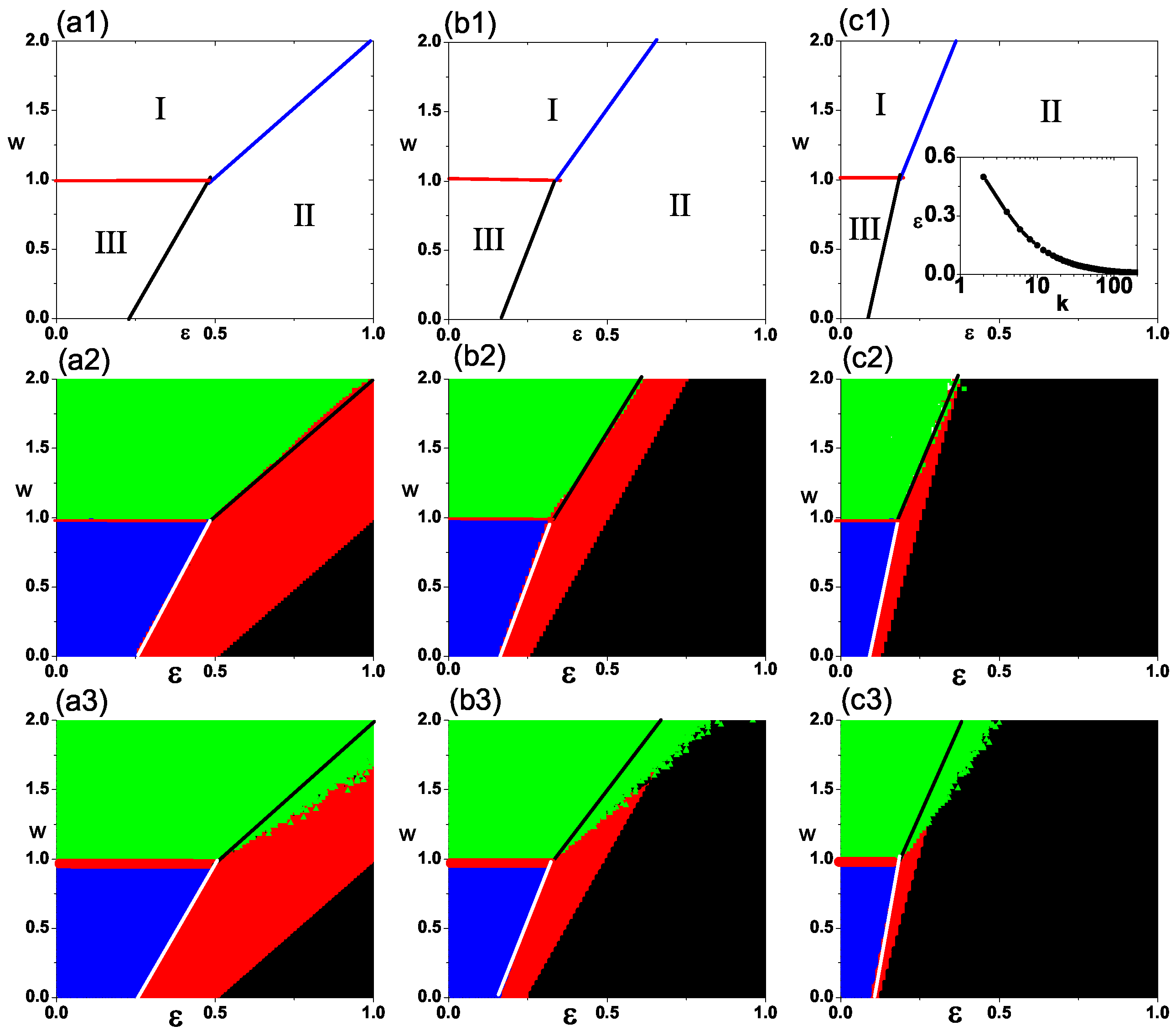
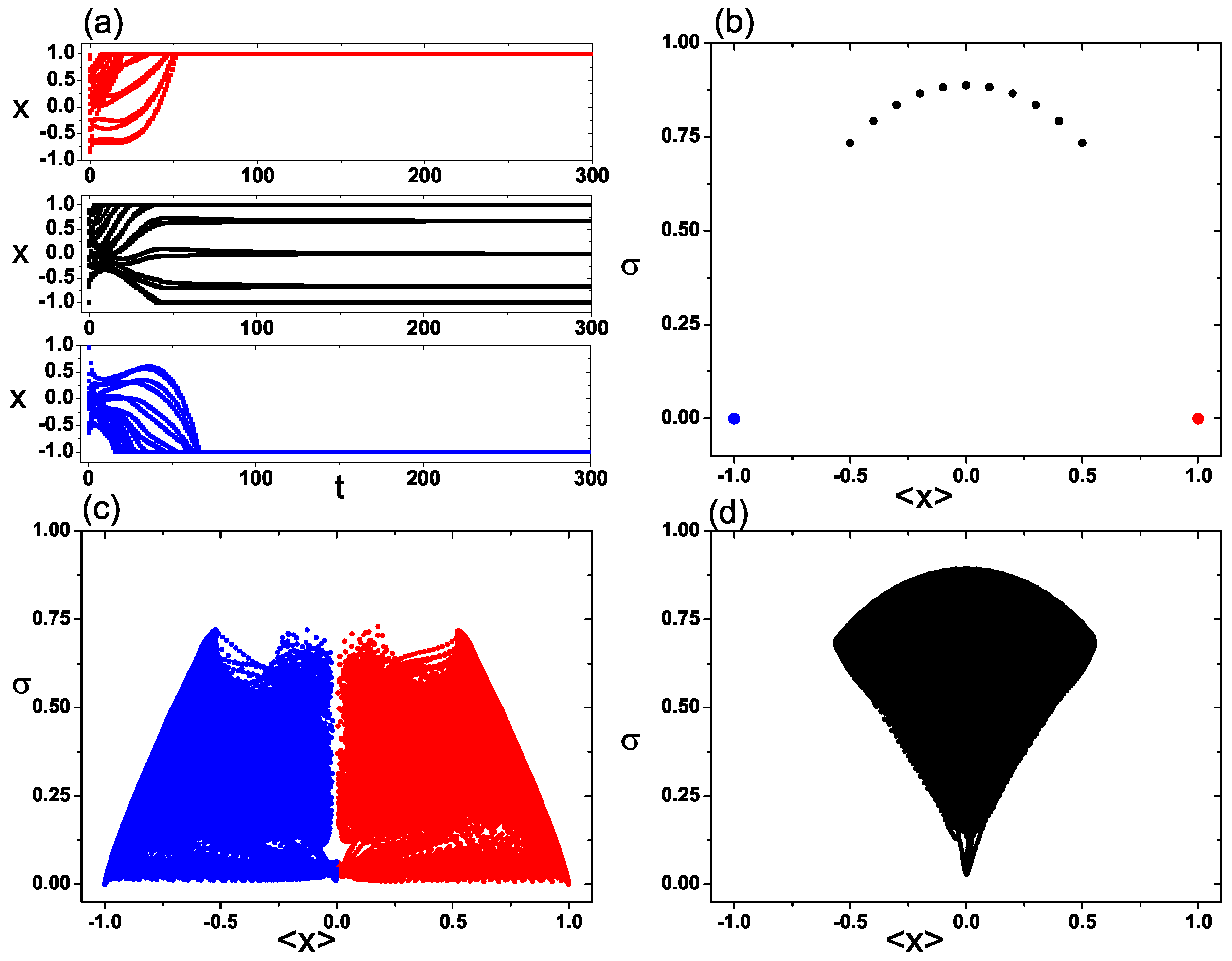
3.1. Phase Diagrams and Opinion Dynamical States

In this section, we numerically investigate the phase diagrams of the model (2) on the plane of ϵ and w in the range of 0 ϵ 1 and 0 w 2 . The results are presented in Figure 1(a2–c2) for the initial opinions randomly chosen from [ 1 , 1 ] and in Figure 1(a3–c3) for the initial opinion randomly chosen from [ 0 , 1 ] , respectively. In these figures, the consensus state region is marked in blue, the frozen state region is marked in green, and the time-dependent state region is marked in red or black. The boundaries w = 1 , ϵ c 1 ( w ) and ϵ c 2 ( w ) are denoted by the red line, the white line and the black line, respectively. In comparison with Figure 1(a1–c1), the simulation results in Figure 1(a2–c2) are in good agreement with the theoretical results. However, Figure 1(a3–c3) show that there is a minor discrepancy between the numerical and the theoretical results. Firstly, the theoretical boundary between the frozen state region and the time-dependent state region is different from the numerical results, which is reflected by the larger frozen state region acquired in the simulations. Secondly, the numerical simulations show that the frozen states in Figure 1(a3–c3) are actually the consensus state, where all agents take the opinion x = 1 (ALL 1 state). For initial opinions x i [ 0 , 1 ] , the discrepancy between the numerical and theoretical results can be explained as follows. Consider the evolution of the mean opinion, which is defined as x = i = 1 N x i / N . The mean opinion is always regarded as the public opinion. When x ( t ) is small, the nonlinear effect induced by the requirement x [ 1 , 1 ] may be ignored. Consequently, Equation (2) suggests that the evolution of the mean opinion follows x ( t + 1 ) = w x ( t ) , which gives rise to x ( t ) = x ( 0 ) w t . Therefore, for initial conditions x i [ 0 , 1 ] , x ( 0 ) > 0 and the consensus state x i = 1 has to be reached. On the other hand, when | λ N | > λ 1 , the nonlinear effect on the evolution of x ( t ) has to be taken into consideration, which prevents x ( t ) from x ( t ) = 1 . The competition between the linear effects and the nonlinear effects on the evolution of x leads to the expansion of the frozen state region.
Figure 2 shows the evolution of the agents’ opinions in different parameter regions. In the frozen state region, three typical states may be realized for arbitrary initial conditions, the frozen fragment state with several clusters composed of opinion 1 and clusters of opinion 1 in Figure 2a, the ALL 1 state in Figure 2b and the ALL 1 state in Figure 2c. The transient spatial–temporal patterns in Figure 2b display a long-wavelength characteristic due to the parameters being close to the λ 1 -induced instability. In contrast, the transient pattern in Figure 2c displays a short-wavelength nature since its parameters are close to the λ N -induced instability. Figure 2d shows the evolution to a consensus state in the consensus region where the final opinion in the state is determined by initial conditions. In the time-dependent state region, two typical time-dependent states are presented in Figure 2e,f. In them, the system evolves to period-2 jump states, in which there exist many tiny opinion clusters and each agent jumps between two opinions, i.e., x i ( t + 1 ) = x i ( t ) . The two states can be distinguished by the fact that there exist other opinions besides opinions 1 and 1 in Figure 2e, while the state in Figure 2f only includes opinions 1 and 1. The former period-2 jump state (Figure 2e exists in the time-dependent region in red in Figure 1, while the latter period-2 jump state (Figure 2f) exists in the time-dependent region in black. The boundary between these two period-2 jump states is given by w ϵ k = 1 , which can be obtained heuristically as follows. We reformulate Equation (2) to be
x i ( t + 1 ) = ( w ϵ k ) x i ( t ) + ϵ k x ( t ) i ¯
where x ( t ) i ¯ denotes the local mean opinion at agent i excluding x i . The first term on the right-hand side accounts for the contribution to x i ( t + 1 ) from agent i himself. When w ϵ k < 1 , it drives x i ( t ) towards ± 1 . The second term accounts for the joint contributions to x i ( t + 1 ) from the neighbors of agent i, which may balance the first term and help agent i to reach other opinions except for 1 and 1 when w ϵ k < 1 is not held.
To further reveal how the model parameters impact the opinion dynamical states, we consider the final opinions held by agents after transients. We also monitor two quantities, σ x and σ T , which are defined as
σ x = lim T + 1 T 0 T 1 N i = 1 N ( x i ( t ) x ( t ) ) 2 d t σ T = 1 N i = 1 N 1 T 0 T ( x i ( t ) x ¯ i ) 2
with x ¯ i = lim T + 1 / T 0 T x i ( t ) d t . σ x ( t ) measures the opinion fluctuation in space, while σ T measures the opinion fluctuation in time. The consensus state is reached when σ x = σ T = 0 . The frozen states require σ x > 0 and σ T = 0 , while σ x > 0 and σ T > 0 are held for the time-dependent states. The results against ϵ for the situations with different k and w are presented in Figure 3. Generally, with the increase in ϵ from zero to 1, σ T stays at zero till ϵ c 2 (or ϵ c 1 ) is reached for w > 1 (or w < 1 ), which signals the frozen states (or consensus states). In the frozen states, nonzero σ x suggests the fragment states that consist of different opinion clusters ( x = 1 or x = 1 ). Beyond ϵ c 2 (or ϵ c 1 ), σ T becomes nonzero, which indicates the time-dependent states.
The final opinions usually fall within a small range, except for the transition between different types of states. The number of final opinions displays non-monotonic behavior against ϵ and, during the process, the final opinions are always symmetrical about x = 0 . Let us take over-confident agents ( w > 1 ) as examples. As illustrated in Figure 3(a1–c1), the number of final opinions first gradually increases from 2 with ϵ and, then, decreases with ϵ gradually to 2 after ϵ c 2 . The number of final opinions in the frozen states and the range of ϵ supporting these states can be acquired based on Equation (12). As discussed above, in the frozen states, the population is composed of opinion 1 clusters and opinion 1 clusters. The opinions different from 1 and 1 only occur at the boundaries of these different opinion clusters. Therefore, the opinion configurations such as ( 1 , 1 ) , ( 1 , 0 , 1 ) , ( 1 , x , x , 1 ) , ( 1 , x , 0 , x , 1 ) , etc., are the typical ones at the boundaries between different clusters. The appearance of the configuration ( 1 , 0 , 1 ) suggests the existence of a frozen state with three opinions, while the appearance of the configuration ( 1 , x , x , 1 ) suggests the existence of a frozen state with four opinions. Bearing these in mind, the number of final opinions in frozen states and the range of ϵ supporting these states can be acquired based on Equation (12). To be specific, we consider k = 2 . For the configuration ( 1 , 1 ) , the model (2) requires ϵ < ( w 1 ) / 2 , which signals the transition from a frozen state with two opinions to a frozen state with three opinions. For the configuration ( 1 , 0 , 1 ) , the state transitions to a state with four final opinions at ϵ = w 1 . For ( 1 , x , x , 1 ) , we can obtain x = ϵ / ( 3 ϵ + 1 w ) and the critical point at ϵ = ( w 1 ) / ( 1 x ) . Since ( w 1 ) / ( 1 x ) is higher than ϵ c 2 for k = 2 , the transition to a frozen fragment state with five opinions does not exist. In addition, the initial conditions play important roles in the opinion distribution before ϵ c 2 . Firstly, although the number of final opinions is determined by given parameters, the distribution of agents on these opinions depends on the initial conditions. Secondly, if the initial opinions are distributed in the range [ 0 , 1 ] or [ 1 , 0 ] , the final states become the ALL 1 (ALL 1 ) consensus state and the frozen fragment states with more than one opinion disappear.

3.2. Finite Size Effects

Finite size effects are a research subject in opinion dynamics when the population size is small. In model (2), the ALL 1 and ALL 1 states are the absorbing states. Once these absorbing states are built, the population cannot escape from them in the absence of external stimuli. For a small population size, the system can be trapped by these absorbing states due to fluctuations in the evolution. To investigate the finite size effects in the model (2), we consider the influence of the population size N on the opinion dynamics at parameters close to the long-wavelength-induced instability of consensus states. Besides frozen fragment states as the steady state, the absorbing states, the ALL 1 state and ALL 1 state, may be realized for uniform random initial conditions in [ 1 , 1 ] due to the finite size effects. We measure the probability p by counting the realizations trapped in the absorbing states for a large number of initial conditions. The results are presented in Figure 4, where p is plotted against N. From this, we can see that increasing N decreases p. p drops to zero when N > 80 , which suggests that the finite size effects may be ignored for N = 100 used in this work. Figure 4 also shows that there exists a critical population size N c below which the absorbing states are always reached. The critical population size N c may be determined by the second largest eigenvalue λ 2 of the matrix P. According to Equation (7), N c has to obey the following equation:
w 1 4 ϵ = j = 1 k / 2 sin 2 ( j π N c ) .
It is interesting to investigate the attraction basins of the absorbing states and frozen states for a small N where finite size effects are prominent. To explore the attraction basins of different opinion dynamical states, we introduce the mean variance space. The mean opinion x is defined as < x > = 1 / N i = 1 N x i , which represents the public opinion. The opinion variance σ is defined as σ = 1 / N i = 1 N ( x i < x > ) 2 , which represents the opinion fluctuation in the population. The mean variance space is a low-dimensional projection of the high-dimensional phase space of opinion dynamics. We consider the over-confident population with w = 1.1 , N = 20 , ϵ = 0.2 and k = 2 . The evolutions in Figure 5a display three frozen states with five final opinions. As mentioned above, the five opinions are symmetrical about x = 0 . Since N = 20 , it is easy to see that, in these frozen states, there are six agents holding opinions other than 1 and 1 and located at the boundaries between one opinion 1 cluster and one opinion 1 cluster. There are 11 different frozen states distinguished by the number of agents falling into the opinion 1 cluster. Figure 5b presents all possible states in the mean variance space, which shows that frozen states possess large variance and a low mean. The attraction basins of the absorbing states are presented in Figure 5c. As shown, the attraction basins of the ALL 1 state and ALL −1 state are symmetrical about x = 0 and x = 0 may serve as the boundary between them. At low variance, positive (or negative) initial public opinions always lead to the ALL 1 state (or ALL 1 state). Treating the sign of x as the inclination of the public opinion, Figure 5c implies that the initial inclination of the public opinion determines the inclination of the final states. Figure 5d presents the attraction basin of the frozen fragment states. As shown, the population with x = 0 always evolves towards these frozen fragment states. For a nonzero public opinion, the population is more likely to evolve towards fragment states if the opinion variance is large. In particular, when σ > 0.73 , all of the initial conditions will lead to these frozen fragment states. In sum, we find that the initial conditions are highly related to the final states for the over-confident population. It is more likely for a neutral population with large variance to evolve into a heterogeneous population.

4. Conclusions and Discussion

In this paper, we construct a non-consensus model, namely the DeGroot-Non-Consensus model, from a consensus model. Based on the social influence model, the new opinion model is proposed by releasing the requirement j = 1 N w i j = 1 and w i j 1 . In the DeGroot-Non-Consensus model, the self-confidence w is never a weight in the social influence model but a parameter characterizing the intra-person information process. Its value is related to the stability of the equilibrium of the intra-person information process and expanded from [ 0 , 1 ] to [ 0 , + ) . Moreover, w can also be regarded as the stubbornness of the agent. The most stubborn agents taking j = 1 N w i j = 1 in the social influence model correspond to the agents taking w = 1 and ϵ = 0 in the new opinion model. However, the zealots in the new opinion model are different. They are agents who tend to become extremists, denoted by w > 1 . Moreover, a nonlinear operation is introduced to describe the phenomenon in which the opinion is limited by the human cognitive limitations around the boundaries.
The opinion dynamics on the regular rings with a series of degrees were studied theoretically and numerically. The linear stability of the consensus state was analyzed and the phase diagrams on the plane of self-confidence w and the convergence ϵ were presented. The parameter plane is divided into three regimes, the consensus states, the frozen fragment states and the time-dependent states. The consensus region is located in the w 1 region with 0 < ϵ < ϵ c 1 . There are two types of consensus, c = i = 1 N x i ( 0 ) / N and c = 0 . The frozen region is located in the w > 1 region with 0 < ϵ < ϵ c 2 . The rest is the time-dependent non-consensus region. In this region, the system evolves to a jump state. The result shows that the non-consensus states occupy the largest parameter space and a limited area is occupied by the consensus states. This supports the widely observed non-consensus states in reality. The area of the non-consensus states increases with the degree k and the convergence ϵ . Once ϵ is large enough, the population eventually evolves to the jump state regardless of its self-confidence. This implies that the under-confident population ( w < 1 ) with the equilibrium of the intra-person information process x * = 0 can become jumping extremists once the convergence ϵ is large enough. We also investigated the finite size effects on opinion dynamics. We found that, for a small population size, a neutral population with large opinion variance is robust to the fluctuations induced by the finite population size.
In sum, the proposed opinion model is a non-equilibrium system. The origin of the non-consensus states is not a settled disagreement pattern, such as the insistence of the initial opinion in the Friedkin and Johnsen model, but an inner nonlinear mechanism. It is the influence of the human cognitive limitations on opinions at the boundaries. Let opinions represent the paradigms; the frozen fragment state can be comprehended as a confrontation of different new paradigms. These new paradigms are caused by two factors. One is the original stable equilibrium losing its stability, and the other is the boundary, which can absorb the opinions x > 1 and x < 1 . The research here shows that such a phenomenon only happens in the population with w > 1 . It is the population organized by the person who has the ability to expand the opinion interval. However, without an initial neutral public opinion, it is also difficult for it to approach the frozen fragment state. The result is consistent with the observations in reality. We hope that the opinion model will be helpful to understand the dynamics of scientific progress and technological evolution, which involve a sequence of periods of stagnation, transitions and paradigm shifts.
Lastly, we focus on the assumptions and limitations of the model. There are two main assumptions. The first assumption is that the opinion space is limited. A nonlinear operation is introduced to ensure the assumption. The joint effect of the nonlinear operation and w i is the origin of the non-consensus states. The nonlinear operation is regarded as a description of the limitation of the cognition. The second assumption is the linear relationship between w i and x i in the intra-personal information process. Actually, the intra-information process is neither a simple process nor a single parameter process. The operation is a simplification. Then, let us discuss the limitations and some related following works. The first limitation is in the model itself. The DeGroot-Non-Consensus model is a deterministic model, while the original DeGroot model is not. P in the original DeGroot model is a stochastic matrix, while P in the DeGroot-Non-Consensus model is a Laplacian matrix. In the following work, we will develop a corresponding probability model. The second limitation is in the investigation of the influence of the topology. The influence of the topology on non-consensus states is an interesting and important problem. Here, we only consider the influence of the degree. The following work will focus on much more complex structures such as scale-free networks and small-world networks, in which there is a distribution of the degree. We hope that the results presented here can support related further investigations.

Author Contributions

Conceptualization, X.Q.; methodology, X.Q.; validation, X.Q. and W.H.; formal analysis, X.Q. and J.Y.; investigation, X.Q.; resources, X.Q.; writing—original draft preparation, X.Q.; writing—review and editing, X.Q., W.H. and J.Y.; visualization, X.Q.; supervision, J.Y.; funding acquisition, X.Q. and W.H. All authors have read and agreed to the published version of the manuscript.

Funding

This work was supported by the National Natural Science Foundation of China under Grant No. 11947061, the Scientific Research Fund of Zhejiang Provincial Education Department (Number: Y202044772) and the Key Research and Development Program of Zhejiang Province (No. 2019C0100).

Data Availability Statement

All data that support the findings of this study are included within the article.

Acknowledgments

X.Q. is grateful for the Scientific Research Fund of Zhejiang Provincial Education Department (Number: Y202044772), the Key Research and Development Program of Zhejiang Province, China under Grant No. 2019C03131 and the Key Research and Development Program of Zhejiang Province, China, under Grant No. 2019C0100, provided to complete this work. W.H. is grateful for the support provided by the National Natural Science Foundation of China under Grant No. 11947061 to complete this work.

Conflicts of Interest

The authors declare that they have no known competing financial interests or personal relationships that could have appeared to influence the work reported in this paper.

References

  1. French, J.R.P. A formal theory of social power. Psychol. Rev. 1956, 63, 181–194. [Google Scholar] [CrossRef] [PubMed]
  2. DeGroot, M.H. Reaching a consensus. J. Am. Stat. Assoc. 1974, 69, 118–121. [Google Scholar] [CrossRef]
  3. Saber, R.O.; Fan, J.A.; Murray, R.M. Consensus and Cooperation in Networked Multi-Agent Systems. Proc. IEEE 2007, 95, 215–233. [Google Scholar] [CrossRef]
  4. Ding, Z.G.; Chen, X.; Dong, Y.C.; Herrera, F. Consensus reaching in social network DeGroot Model: The roles of the Self-confidence and node degree. Inf. Sci. 2019, 486, 62–72. [Google Scholar] [CrossRef]
  5. Sznajd-Weron, K.; Sznajd, J. Opinion evolution in closed community. Int. J. Mod. Phys. C 2000, 11, 1157–1165. [Google Scholar] [CrossRef]
  6. Galam, S. Minority opinion spreading in random geometry. Eur. Phys. J. B 2002, 25, 403–406. [Google Scholar] [CrossRef]
  7. Friedkin, N.E.; Johnsen, E.C. Social influence networks and opinion change. Adv. Group Process 1999, 16, 1–29. [Google Scholar]
  8. Friedkin, N.E.; Proskurnikov, A.V.; Tempo, R.; Parsegov, S.E. Network science on belief system dynamics under logic constraints. Science 2016, 354, 321–326. [Google Scholar] [CrossRef]
  9. Deffuant, G.; Neau, D.; Amblard, F.; Weisbuch, G. Mixing beliefs among interacting agents. Adv. Compl. Sys. 2000, 3, 87–98. [Google Scholar] [CrossRef]
  10. Hegselmann, R.; Krause, U. Opinion dynamics and bounded confidence models, analysis, and simulation. J. Artif. Soc. Soc. Simul. 2002, 5, 1–33. [Google Scholar]
  11. Castellano, C.; Fortunato, S.; Loreto, V. Statistical physics of social dynamics. Rev. Mod. Phys. 2009, 81, 591. [Google Scholar] [CrossRef]
  12. Shao, J.; Havlin, S.; Stanley, H.E. Dynamic opinion model and invasion percolation. Phys. Rev. Lett. 2009, 103, 018701.1–018701.4. [Google Scholar] [CrossRef] [PubMed]
  13. Wu, Y.; Du, Y.J.; Chen, X.L.; Li, X.Y. Newly exposed conflicting news based network opinion reversal. Acta Phys. Sin. 2016, 65, 030502. [Google Scholar] [CrossRef]
  14. Hou, Z.; Bin, H. Impact of information on public opinion reversal-An agent based model. Phys. A 2018, 512, 578–587. [Google Scholar]
  15. Telba, Z.I.; Pereira, c.A.d.B.; Ram, C.T. Analysis of opinion swing: Comparison of two correlated proportions. Am. Stat. 2000, 54, 57–62. [Google Scholar]
  16. Pearson, P.T.; Cooper, C.I. Using self organizing maps to analyze demographics and swing state voting in the 2008 U.S. Presidential Election. In Proceedings of the Artificial Neural Networks in Pattern Recognition (ANNPR) 2012, Trento, Italy, 17–19 September 2020. [Google Scholar]
  17. Akgiray, V.; Booth, G.G. Mixed diffusion-jump process modeling of exchange rate movements. Rev. Econ. Stat. 1988, 70, 631–637. [Google Scholar] [CrossRef]
  18. Fu, G.; Zhang, W.; Li, Z. Opinion dynamics of modified Hegselmann-Krause model in a group-based population with heterogenenous bounded confidence. Phys. A 2015, 419, 558–565. [Google Scholar] [CrossRef]
  19. Ghaderi, J.; Srikant, R. Opinion dynamics in social networks with stubborn agents: Equilibrium and convergence rate. Automatica 2014, 50, 3209–3215. [Google Scholar] [CrossRef]
  20. Olshevsky, A.; Tsitsiklis, J.N. Convergence speed in distributed consensus and averaging. SIAM J. Control Optim. 2009, 48, 33–55. [Google Scholar] [CrossRef]
  21. Han, W.; Huang, C.; Yang, J.Z. Opinion clusters in a modified Hegselmann-Krause model with heterogeneous bounded confidences and stubbornness. Phys. A 2019, 531, 121791. [Google Scholar] [CrossRef]
  22. Bearden, W.O.; Hardesty, D.M.; Rose, R.L. Consumer self-confidence: Refinements in conceptualization and measurement. J. Consum. Res. 2001, 28, 121–134. [Google Scholar] [CrossRef]
  23. Koehler, D.J. Explanation, imagination, and confidence in judgment. Am. Psychol. Assoc. 1991, 110, 499–519. [Google Scholar] [CrossRef] [PubMed]
  24. Bandura, A.; Wood, R. Effect of perceived controllability and performance standards on selfregulation of complex decision making. J. Personal. Soc. Psychol. 1989, 56, 805–814. [Google Scholar] [CrossRef]
  25. Ghosh, D.; Ray, M. Risk, ambiguity, and decision choice: Some additional evidence. Decis. Sci. 1997, 28, 81–104. [Google Scholar] [CrossRef]
  26. Adams, J.K.; Adams, P.A. Realism of confidence judgments. Psychol. Rev. 1961, 68, 33–45. [Google Scholar] [CrossRef] [PubMed]
  27. Fonseca, C.; Pettitt, J.; Woollard, A.; Rutherford, A.; Bickmore, W.; Ferguson-Smith, A.; Hurst, L.D. People with more extreme attitudes towards science have self-confidence in their understanding of science, even if this is not justified. PLoS Biol. 2023, 21, e3001915. [Google Scholar] [CrossRef]
  28. Van Prooijen, J.W.; Krouwel, A.P.M. Psychological Features of Extreme Political Ideologies. Curr. Dir. Psychol. Sci. 2019, 28, 159–163. [Google Scholar] [CrossRef]
  29. Chuang, S.C.; Cheng, Y.H.; Chang, C.J.; Chiang, Y.T. The impact of self-confidence on the compromise effect. Int. J. Psychol. 2013, 48, 660–675. [Google Scholar] [CrossRef]
Figure 1. The phase diagrams on the plane of the self-confidence w and the convergence ϵ . (a1c1) The theoretical results for k = 2 , k = 4 and k = 8 . Frozen fragment states in region I, time−dependent states in region II and consensus states in region III. w = 1 in red, ϵ c 1 in black and ϵ c 2 in blue. The inset in (c1) shows ϵ c against k at w = 1 . (a2c2) The numerical results with initial opinions randomly distributed in [ 1 , 1 ] for k = 2 , k = 4 and k = 8 . (a3c3) The numerical results with initial opinions randomly distributed in [ 0 , 1 ] for k = 2 , k = 4 and k = 8 . Different colors indicate different opinion dynamical regions; the consensus region in blue, the frozen region in green, the region of jump states with other opinions besides 1 and −1 in red and the region of jump states consisting of only opinions 1 and −1 in black.
Mathematics 12 00228 g001
Figure 2. The evolution of different opinion dynamical states at k = 8 . (a) The frozen fragment state at ϵ = 0.2 and w = 1.5 . (b) ALL −1 state at ϵ = 0.13 and w = 1.13 . (c) ALL 1 state at ϵ = 0.2 and w = 1.15 . (d) Consensus state at ϵ = 0.36 and w = 0.6 . (e) The jump states with other opinions besides 1 and −1 at ϵ = 0.19 and w = 0.87 . (f) The jump state with only 1 and −1 at ϵ = 0.7 and w = 1.5 .
Mathematics 12 00228 g002
Figure 3. The transition scenarios against the convergence ϵ . (a1c1) The transition scenarios with w = 1.5 for k = 2 , k = 4 and k = 8 . (a2c2) The transition scenarios with w = 1 for k = 2 , k = 4 and k = 8 . (a3c3) The transition scenarios with w = 0.5 for k = 2 , k = 4 , and k = 8 . The opinions in the final states in black, σ T in blue and σ x in red.
Mathematics 12 00228 g003
Figure 4. The probability p of finding the absorbing states is plotted against the population size N for ϵ = 0.1 (black), ϵ = 0.2 (green) and ϵ = 0.3 (green). Other parameters w = 1.1 and k = 2 .
Mathematics 12 00228 g004
Figure 5. (a) The evolution towards different final opinion dynamical states in over−confident population with small population size. (b) The final opinion dynamical states, ALL 1 state in red, ALL −1 state in blue and frozen fragment states in black, are presented in the mean variance space. (c) The attraction basins of ALL 1 state (red) and ALL −1 state (blue). (d) The attraction basins of frozen fragment states. w = 1.1 , ϵ = 0.2 , k = 2 , and N = 20 .
Mathematics 12 00228 g005
Disclaimer/Publisher’s Note: The statements, opinions and data contained in all publications are solely those of the individual author(s) and contributor(s) and not of MDPI and/or the editor(s). MDPI and/or the editor(s) disclaim responsibility for any injury to people or property resulting from any ideas, methods, instructions or products referred to in the content.

