The Shape Parameter in the Shifted Surface Spline—A Sharp and Friendly Approach

Abstract

This is a continuation of our previous study on the shape parameter contained in the shifted surface spline. We insist that the data points be purely scattered without meshes and the domain can be of any shape when conducting function interpolation by shifted surface splines. We also endeavor to make our approach easily accessible for scientists, not only mathematicians. However, the space of interpolated functions is smaller than that used before, leading to sharper function approximation. This function space has particular significance in numerical partial differential equations, especially for equations whose solutions lie in Sobolev space. Although the Fourier transform is deeply involved, scientists without a background in Fourier analysis can easily understand and use our approach.

1. Introduction

Shifted surface splines are a kind of radial basis function (RBF) defined by

$$\begin{array}{ccc}\hfill h\left(x\right)& :=& \left\{\begin{array}{cc}{(-1)}^{\lceil m\rceil }{\left(\right|x|}^2+c^2{)}^{\frac{\lambda }{2}},\lambda \in {\mathbb{Z}}_{+},\lambda \mathrm{odd},m=\frac{\lambda }{2}\hfill & \mathrm{if} n \mathrm{is} \mathrm{odd},\hfill \\ {(-1)}^m{\left(\right|x|}^2+c^2{)}^{\frac{\lambda }{2}}log{\left(\right|x|}^2+c^2{)}^{\frac{1}{2}},\lambda \in {\mathbb{Z}}_{+},\lambda \mathrm{even},m=1+\frac{\lambda }{2}\hfill & \mathrm{if} n \mathrm{is} \mathrm{even},\hfill \end{array}\right.\hfill \end{array}$$

(1)

where $x\in {\mathbb{R}}^n$, $c>0$; $\left|x\right|$ stands for the Euclidean norm of x; log denotes the natural logarithm; $\lceil m\rceil$ denotes the smallest integer not less than m; and $\lambda ,c$ are constants determined by the user. The primary concern of this paper is the optimal choice of c, called the shape parameter.

The origin and significance of shifted surface splines were discussed in Luh [1], and we omit them here. The generalized Fourier transform of $h\left(x\right)$ will be needed and is of the form

$$\begin{array}{c}\hfill \widehat{h}\left(\xi \right)={l(\lambda ,n)\left|\xi \right|}^{-\lambda -n}{\tilde{\mathcal{K}}}_{\frac{n+\lambda }{2}}\left(c\right|\xi \left|\right),\end{array}$$

(2)

where $l(\lambda ,n)$ is a constant depending on $\lambda$ and n (see Luh [1]), and ${\tilde{\mathcal{K}}}_{\nu }\left(t\right):=t^{\nu }{\mathcal{K}}_{\nu }\left(t\right),{\mathcal{K}}_{\nu }$ is the modified Bessel function of the second kind (Abramowitz et al. [2]).

Note that the odd-dimensional and even-dimensional parts of (1) share the same Fourier transform, and the former is just the multiquadrics. This means that, in some sense, multiquadrics are just a kind of shifted surface spline.

Based on an established theory of radial basis functions (Wendland et al. [3,4,5,6]), for any set of data points $(x_1,y_1),\dots ,(x_N,y_N)$, where $x_1,\dots ,x_N$ are arbitrary points in ${\mathbb{R}}^n$ and $y_1\dots ,y_N$ are arbitrary real numbers, one can always construct a unique interpolating function passing through these data points, with a mild requirement that $x_1,\dots ,x_N$ be polynomially nondegenerate. The interpolator is of the form

$$s\left(x\right):=\sum _{j=1}^N{c}_{j}h(x-x_j)+p\left(x\right)$$

(3)

where $c_1,\dots ,c_N$ are constants to be determined, and p is a polynomial of degree $\le m-1$. The coefficients of $p\left(x\right)$ are simultaneously determined by solving the system of linear equations required by the interpolation. In this paper, we will let $n=2$ and $\lambda =2$. Hence, $m=2$, and $p\left(x\right)$ is a polynomial of degree one.

Computationally, the most time-consuming step of the interpolation is solving the system of linear equations. As for the quality of the interpolation, it greatly depends on the choice of the shape parameter c. For odd dimensions, the choice of the shape parameter has been deeply studied in Luh [7]. For even dimensions, we already have two papers Luh [1,8], where [8] establishes a theoretically rigorous and practically useful approach for evenly spaced data points distributed in simplices, and [1] deals with scattered data points from functions belonging to a function space denoted by $E_{\sigma }$. In this paper we will focus on another space defined as follows.

Definition 1.

For any $\sigma >0$, define

$$B_{\sigma }:=\{f\in L^2\left({\mathbb{R}}^n\right):|\widehat{f}\left(\xi \right)|=0if|\xi |>\sigma \},$$

where $\widehat{f}$ denotes the Fourier transform of f.

This space plays an important role in the RBF collocation method of solving PDEs. As pointed out in Luh [7], each function in a Sobolev space can be approximated by a $B_{\sigma }$ function, and each $B_{\sigma }$ function can be approximated by a function of the form (3). Since many important PDEs have solutions lying in a Sobolev space, one can use the RBF to handle PDEs well, as long as the solution lies in a Sobolev space. Consequently, the choice of the shape parameter c contained in $h\left(x\right)$ will be very influential not only for function interpolation, but also for numerical PDEs.

As for the choice of the shape parameter, we totally discard the trial-and-error methods widely used by experts in this field. Instead, we predict its optimal value directly by theory. No search is needed. Hence, no algorithm is involved. This means that finding a suitable shape parameter in practical applications will become computationally very efficient. Of course, the reliability of our final results will be strictly investigated by experiments.

2. Materials and Methods

Our theory is based on function interpolation. The basic idea is that if the shape parameter c is chosen well, the interpolation error bound should be very small. The c value minimizing the error bound is supposed to be the optimal choice. In fact, we have already successfully established such a theory for function interpolation with a simplex domain and interpolation points evenly spaced in the domain, as can be seen in Luh [8].

We are reluctant to refer too much to the complicated theory of [8]. However, in order to make this paper self-contained, some necessary ingredients still have to be introduced here.

Our strict theory asks that the interpolation domain is a simplex. Each n-dimensional simplex in ${\mathbb{R}}^n$ has $n+1$ vertices. Each point in the simplex can be expressed as a linear combination of the vertices, with non-negative coefficients, called its barycentric coordinates. The sum of the barycentric coordinates is equal to 1. Simplices are the fundamental geometric objects used in [8], where the distribution of the interpolation points in a simplex is described according to a rule so that they are evenly spaced. In the rule, there is a parameter k, called the degree. The number k is proportional to the number of points. All these details can be seen in Fleming [9]. As mentioned in [8], the number of interpolation points of degree k in a simplex is equal to the dimension of ${\mathbb{P}}_k^n$, the space of n-variate polynomials of a degree less than or equal to k. In this subsection, we use N to denote this number, that is, $N:=dim{\mathbb{P}}_k^n$.

Besides simplices and the distribution of data points, two constants $\rho$ and ${\Delta }_0$ should also be mentioned. They are defined in a very complicated way and are completely determined by n and $\lambda$ in Equation (1). In order to save space, we refer the reader directly to [8].

The interpolated functions belong to the native space ${\mathcal{C}}_{h,m}$. In order to avoid a digression, we refer the reader to Madych et al. [5,6] and Wendland [3] for its complicated definition. The interpolation error of the native space functions from shifted surface splines is governed by the following theorem.

Theorem 1.

Let h be as in Equation (1). For any positive number $b_0$, there exist positive constants ${\delta }_0,d_1,C,\omega ,0<\omega <1$, completely determined by h and $b_0$, such that for any n-dimensional simplex $Q_0$ of diameter $b_0$, any $f\in {\mathcal{C}}_{h,m}$, and any $0<\delta \le {\delta }_0$, there exists a number r satisfying the property that $1/\left(3C\right)\le r\le b_0$, and for any n-dimensional simplex Q of diameter r, $Q\subseteq Q_0$, there is an interpolating function $s(·)$ as defined in Equation (3), such that

$$|f\left(x\right)-s\left(x\right)|\le d_1\sqrt{\delta }{\left(\omega \right)}^{1/\delta }{\parallel f\parallel }_h$$

(4)

for all x in Q, where C is defined by

$$C:=max\left\{8{\rho }^{\prime },2/\left(3b_0\right)\right\},{\rho }^{\prime }:=\rho /c,$$

and c was defined in Equation (1). The function $s(·)$ interpolates f at centers that are evenly spaced points of degree $k-1$ in Q, with $k=\lceil \frac{r}{\delta }\rceil$. Here, ${\parallel f\parallel }_h$ is the h-norm of f in the native space.

The numbers ${\delta }_0,d_1$, and ω are given by ${\delta }_0:=1/\left[3C(m+1)\right]$, where m was defined in Equation (1),

$$d_1:=2^{-7/4}{3}^{1/2}\sqrt{l(\lambda ,n)}{\pi }^{-1/4}\sqrt{n{\alpha }_n}{c}^{\lambda /2}\sqrt{{\Delta }_0}\sqrt{C}$$

where λ is as in Equation (1), $l(\lambda ,n)$ was defined in Equation (2), ${\alpha }_n$ is the volume of the unit ball in ${\mathbb{R}}^n$, and $\omega :={\left(2/3\right)}^{1/\left(3C\right)}$.

Remark 1.

In the preceding theorem, the most noteworthy parameter is δ, which appears in Formula (4). This parameter indicates the number of data points used. The smaller δ is, the more data points will be used. As $\delta \to 0$, the upper bound in (4) will converge to zero. Hence, δ functions as the well-known fill distance. We cannot say they are the same, although they are quite alike. Hence, one should be careful when using this theorem.

The error bound (4) cannot be used to choose the shape parameter c directly before its relation with c is made transparent. For this, we will adopt the function space $B_{\sigma }$ defined in Definition 1, which is a subset of ${\mathcal{C}}_{h,m}$.

By Corollary 2.5 of Luh [8], if $f\in B_{\sigma }$, the inequality (4) can be transformed into

$$|f\left(x\right)-s\left(x\right)|\le C_B{c}^{(1+\lambda -n)/4}\sqrt{C}{e}^{c\sigma /2}{\left(\frac{2}{3}\right)}^{1/\left(3C\delta \right)}\sqrt{\delta }{\parallel f\parallel }_{L^2},$$

(5)

where $C_B:={\sigma }^{(1+n+\lambda )/4}{\left(2\pi \right)}^{-n}\sqrt{6n{\alpha }_n{\Delta }_0{\left(16\pi \right)}^{-1}m!}$. It can be clearly seen that the upper bound in (5) contains a function of c. Let us denote it by MN(c). Then,

$$\mathrm{M}\mathrm{N}\left(c\right)=c^{(1+\lambda -n)/4}\sqrt{C}{e}^{c\sigma /2}{\left(\frac{2}{3}\right)}^{1/\left(3C\delta \right)}.$$

(6)

For a fixed $b_0$,

$$C=\left\{\begin{array}{cc}\frac{8\rho }{c}\hfill & \mathrm{if} c_0\le c\le c_1,\hfill \\ \\ \frac{2}{3b_0}\hfill & \mathrm{if} c_1\le c<\infty ,\hfill \end{array}\right.$$

where $c_0:=24\rho (m+1)\delta$ and $c_1:=12\rho b_0$ (here, $c_1$ is different from the $c_1$ in (3)). Hence,

$$\mathrm{M}\mathrm{N}\left(c\right):=\left\{\begin{array}{cc}\sqrt{8\rho }{c}^{\frac{\lambda -n-1}{4}}{e}^{c[\sigma /2+ln(2/3)/(24\rho \delta \left)\right]}\hfill & \mathrm{if} c_0\le c\le c_1,\hfill \\ \\ \sqrt{\frac{2}{3b_0}}{c}^{\frac{1+\lambda -n}{4}}{e}^{c\sigma /2}{\left(\frac{2}{3}\right)}^{\frac{b_0}{2\delta }}\hfill & \mathrm{if} c_1\le c<\infty .\hfill \end{array}\right.$$

(7)

In fact, Formulae (5), (6) and (7) can be found in [8]. We restated them just to make this paper easier to understand.

The graph of the MN function can be easily and efficiently sketched using Mathematica or Matlab. A typical example is shown in Figure 1.

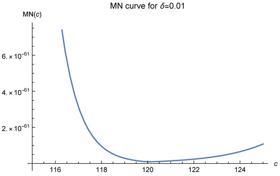
Figure 1. Here, $n=2,\lambda =2,\sigma =1,$ and $b_0=10$.

We assert that for $f\in B_{\sigma }$, the optimal value of c is the value minimizing $\mathrm{M}\mathrm{N}\left(c\right)$. Although in (7) it is required that $c\ge c_0$, a large number of experiments have shown that the true optimal values never lie in the interval $(0,c_0)$. Hence, we have essentially dealt with the entire interval $(0,\infty )$.

The main purpose of this paper is to extend our theory to arbitrary domain shapes and scattered data points. This means that two severe requirements in Luh [8] will be relaxed. Firstly, the interpolation domain need not be a simplex. Secondly, the centers (interpolation points) need not be evenly spaced. The reason for this is that the crucial functions defined in (1) and (3) are continuous, and the relaxation will greatly relieve the pain of using the MN function to choose the c value optimally. For this, we still use the MN function defined in (7) to choose c but interpret $b_0$ just as the diameter of the domain and consider $\delta$ to be just a parameter inversely proportional to the number of data points used. The remaining task is to test this by experiments.

Another key point is that, here, the function space $B_{\sigma }$ is just a subset of another space $E_{\sigma }$ adopted by Luh [1]. Hence, the error bound presented in this paper is sharper than that of [1]. This means that the interpolation here should be more accurate than that in [1].

3. Results

3.1. 2D Experiment

Here, we totally discard the severe restriction that the domain should be a simplex and let it be a square in ${\mathbb{R}}^2$ with vertices $(0,0),(10,0),(10,10)$, and $(0,10)$. The space of the interpolated functions is $B_{\sigma }$, defined in Definition 1, with $\sigma =0.1$. The domain square is denoted by $\mathsf{\Omega }$ and has a diameter of $10\sqrt{2}$. Hence, the parameter $b_0$ in the MN function (7) is equal to $10\sqrt{2}$. We let $\lambda =2$ in the shifted surface spline $h\left(x\right)$ defined in (1). Hence, the parameter $\rho$ in the MN function is equal to 1 according to Definition 2.1 (b) in Luh [8]. The interpolated function is defined by

$$f(x,y):=\left[\frac{sin(\sigma x/\sqrt{2})}{\sigma x/\sqrt{2}}\right]·\left[\frac{sin(\sigma y/\sqrt{2})}{\sigma y/\sqrt{2}}\right]$$

which can be easily shown to be a member of $B_{\sigma }$. Here, we let $\frac{sinz}{z}:=1$ if $z=0$. The interpolating function $s\left(x\right)$ defined in (3) is now of the form

$$s(x,y):=\sum _{j=1}^N{c}_{j}h(x-x_j,y-y_j)+c_{N+1}x+c_{N+2}y+c_{N+3}$$

since the polynomial $p\left(x\right)$ in (3) should be of degree $m-1=1+\frac{\lambda }{2}-1=1$ in ${\mathbb{R}}^2$.

In order to choose the shape parameter c optimally in the shifted surface spline $h(x,y)$, we must analyze the MN curves first. In this experimental setting, the corresponding MN curves are presented in Figure 2, Figure 3, Figure 4, Figure 5 and Figure 6.

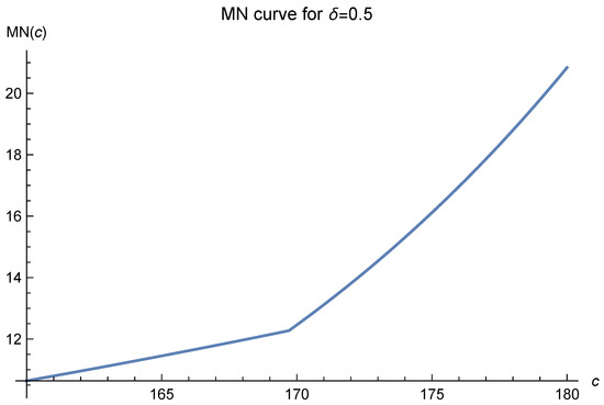
Figure 2. Here, $n=2,\lambda =2,\sigma =0.1,$ and $b_0=10\sqrt{2}$.

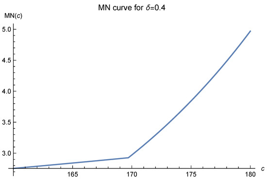
Figure 3. Here, $n=2,\lambda =2,\sigma =0.1,$ and $b_0=10\sqrt{2}$.

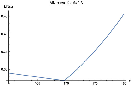
Figure 4. Here, $n=2,\lambda =2,\sigma =0.1,$ and $b_0=10\sqrt{2}$.

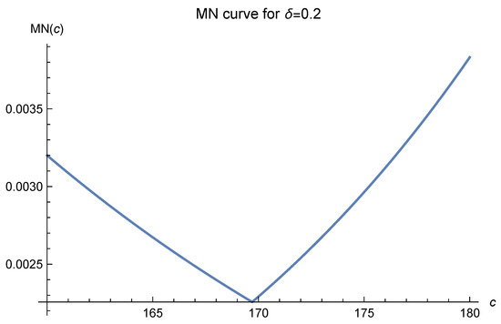
Figure 5. Here, $n=2,\lambda =2,\sigma =0.1,$ and $b_0=10\sqrt{2}$.

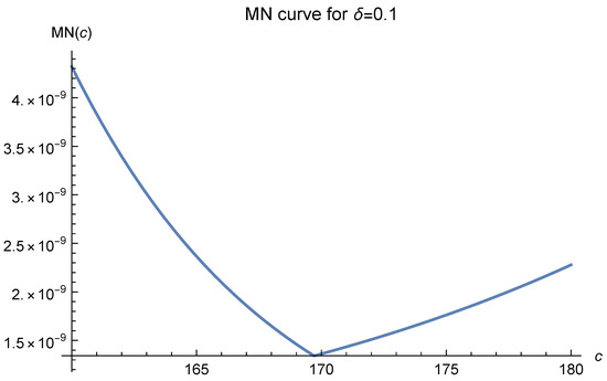
Figure 6. Here, $n=2,\lambda =2,\sigma =0.1,$ and $b_0=10\sqrt{2}$.

In these figures, it is clearly seen that the optimal values of c tend to move to 170 and are fixed there as the $\delta$, which is inversely proportional to the number of data points, decreases. This strongly suggests that one should choose $c=170$ as the optimal value. The remaining task is to test this by experiments.

The test points are a $21\times 21$ grid in the domain square $\mathsf{\Omega }$. In order to measure the quality of the approximation, we define the root-mean-square error at the 441 points as

$$\mathrm{RMS}:=\sqrt{\sum _{j=1}^{N_t}{|s(x_j,y_j)-f(x_j,y_j)|}^2/N_t}$$

where $N_t=441$.

We use N to denote the number of interpolation points, as in (3), which are scattered in the domain without meshes. In the process of building the interpolating function, solving a system of linear equations is necessary. The condition number corresponding to the linear system is denoted by COND. As will be seen, the COND is very sensitive to the number N of data points used and the value of c. Also, as is well known, the condition numbers in the RBF approach may be very large. The ill-conditioning in our experiments was overcome by the arbitrarily precise computer software Mathematica (https://www.wolfram.com/mathematica/). We always adopted enough effective digits in the process of the computation. For example, if the condition number was $3.6\times {10}^{81}$, we adopted 120 effective digits to the right of the decimal point for each step of the calculation. Hence, the results obtained are reliable. The time efficiency was not a problem. In the experiments, solving a linear system always took less than one second, even if ill-conditioning was controlled in this way.

We tried $N=40,50,60,70$, and 80 first. The results are presented in Table 1, Table 2, Table 3, Table 4 and Table 5, where the optimal values of c are marked by the symbol *.

Table 1. $N=40,N_t=441$.

c	100	170 *	200	300	400
RMS	$1.4\times {10}^{-10}$	$1.1\times {10}^{-10}$	$1.65\times {10}^{-10}$	$2.8\times {10}^{-10}$	$3.2\times {10}^{-10}$
COND	$1.3\times {10}^{28}$	$6.9\times {10}^{31}$	$9.5\times {10}^{32}$	$6.6\times {10}^{35}$	$6.9\times {10}^{37}$
c	500	600	700	800	1000
RMS	$3.5\times {10}^{-10}$	$3.6\times {10}^{-10}$	$3.67\times {10}^{-10}$	$3.72\times {10}^{-10}$	$3.8\times {10}^{-10}$
COND	$2.9\times {10}^{39}$	$4.9\times {10}^{40}$	$5.9\times {10}^{41}$	$5.1\times {10}^{42}$	$1.9\times {10}^{44}$
c	3000	6000
RMS	$3.9\times {10}^{-10}$	$3.9\times {10}^{-10}$
COND	$9.3\times {10}^{51}$	$6.6\times {10}^{56}$

Table 2. $N=50,N_t=441$.

c	100	150	160 *	165	170
RMS	$1.3\times {10}^{-11}$	$2.4\times {10}^{-12}$	$2.35\times {10}^{-12}$	$2.44\times {10}^{-12}$	$2.6\times {10}^{-12}$
COND	$4.2\times {10}^{31}$	$7.1\times {10}^{34}$	$2.3\times {10}^{35}$	$4.0\times {10}^{35}$	$6.9\times {10}^{35}$
c	200	300	400	500	600
RMS	$4.3\times {10}^{-12}$	$1.0\times {10}^{-11}$	$1.3\times {10}^{-11}$	$1.5\times {10}^{-11}$	$1.6\times {10}^{-11}$
COND	$1.3\times {10}^{37}$	$2.1\times {10}^{40}$	$4.0\times {10}^{42}$	$2.3\times {10}^{44}$	$6.3\times {10}^{45}$
c	700	800	1000	3000	5000
RMS	$1.67\times {10}^{-11}$	$1.71\times {10}^{-11}$	$1.76\times {10}^{-11}$	$1.84\times {10}^{-11}$	$1.85\times {10}^{-11}$
COND	$1.0\times {10}^{47}$	$1.2\times {10}^{48}$	$6.7\times {10}^{49}$	$3.0\times {10}^{58}$	$3.1\times {10}^{62}$

Table 3. $N=60,N_t=441$.

c	100	150	160	168	170
RMS	$4.7\times {10}^{-13}$	$1.23\times {10}^{-13}$	$6.56\times {10}^{-14}$	$2.985\times {10}^{-14}$	$2.259\times {10}^{-14}$
COND	$8.7\times {10}^{35}$	$3.3\times {10}^{39}$	$1.2\times {10}^{40}$	$3.2\times {10}^{40}$	$4.1\times {10}^{40}$
c	172	175 *	180	190	200
RMS	$1.652\times {10}^{-14}$	$1.2\times {10}^{-14}$	$2.0\times {10}^{-14}$	$4.5\times {10}^{-14}$	$6.57\times {10}^{-14}$
COND	$5.2\times {10}^{40}$	$7.4\times {10}^{40}$	$1.3\times {10}^{41}$	$3.9\times {10}^{41}$	$1.1\times {10}^{42}$
c	300	500	1000	3000	6000
RMS	$1.4\times {10}^{-13}$	$1.54\times {10}^{-13}$	$1.62\times {10}^{-13}$	$1.65\times {10}^{-13}$	$1.65\times {10}^{-13}$
COND	$4.0\times {10}^{45}$	$1.2\times {10}^{50}$	$1.4\times {10}^{56}$	$5.7\times {10}^{65}$	$6.5\times {10}^{71}$

Table 4. $N=70,N_t=441$.

c	100	170	175	180	185
RMS	$3.1\times {10}^{-14}$	$4.76\times {10}^{-15}$	$4.12\times {10}^{-15}$	$3.75\times {10}^{-15}$	$3.56\times {10}^{-15}$
COND	$4.4\times {10}^{36}$	$5.5\times {10}^{41}$	$1.0\times {10}^{42}$	$1.9\times {10}^{42}$	$3.6\times {10}^{42}$
c	190	195	200 *	300	400
RMS	$3.47\times {10}^{-15}$	$3.4\times {10}^{-15}$	$3.3\times {10}^{-15}$	$7.7\times {10}^{-15}$	$1.6\times {10}^{-14}$
COND	$6.4\times {10}^{42}$	$1.1\times {10}^{43}$	$2.0\times {10}^{43}$	$1.6\times {10}^{47}$	$9.4\times {10}^{49}$
c	500	600	1000	3000	6000
RMS	$2.1\times {10}^{-14}$	$2.4\times {10}^{-14}$	$2.9\times {10}^{-14}$	$3.2\times {10}^{-14}$	$3.2\times {10}^{-14}$
COND	$1.3\times {10}^{52}$	$7.5\times {10}^{53}$	$6.1\times {10}^{58}$	$2.2\times {10}^{69}$	$1.0\times {10}^{76}$

Table 5. $N=80,N_t=441$.

c	100	150	170  *	200	300
RMS	$4.4\times {10}^{-15}$	$1.5\times {10}^{-15}$	$1.0\times {10}^{-16}$	$2.4\times {10}^{-16}$	$4.2\times {10}^{-16}$
COND	$1.8\times {10}^{40}$	$6.2\times {10}^{44}$	$7.1\times {10}^{45}$	$1.0\times {10}^{47}$	$1.1\times {10}^{52}$
c	400	500	600	700	800
RMS	$1.9\times {10}^{-15}$	$3.0\times {10}^{-15}$	$3.7\times {10}^{-15}$	$4.2\times {10}^{-15}$	$4.5\times {10}^{-15}$
COND	$1.2\times {10}^{55}$	$2.6\times {10}^{57}$	$2.1\times {10}^{59}$	$8.9\times {10}^{60}$	$2.2\times {10}^{62}$
c	900	1000	2000	3000	5000
RMS	$4.7\times {10}^{-15}$	$4.9\times {10}^{-15}$	$5.4\times {10}^{-15}$	$5.5\times {10}^{-15}$	$5.6\times {10}^{-15}$
COND	$3.8\times {10}^{63}$	$4.9\times {10}^{64}$	$9.0\times {10}^{71}$	$1.6\times {10}^{76}$	$3.6\times {10}^{81}$

In these tables, it is clearly seen that the optimal values of c are always around 170, as predicted by the theory. We were not surprised that the predictions were not as accurate as those in Luh [8]. The main reason is that some strict requirements in [8] were relaxed in this paper. However, the RMS values obtained by letting $c=170$ were all very good and very close to the smallest values. From the viewpoint of practical applications, our approach should be quite reliable and useful.

Unfortunately, the MN curves may be misleading when $\delta$, which indicates the number of data points used, is too large or too small. If $\delta$ is too large, the number of data points used is not sufficient to support the reliability of the prediction. In general, the MN curves are reliable only when enough data points are used. However, too many data points may also weaken the reliability, although this does not happen often, as explained in the next subsection.

3.2. The Limitation of the MN Curve Approach

If we further decrease $\delta$, i.e., increase the number of data points, in Figure 6, the MN curves will tend to be flat to the right of $c=170$. We show this in Figure 7, Figure 8, Figure 9, Figure 10, Figure 11 and Figure 12.

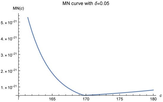
Figure 7. Here, $n=2,\lambda =2,\sigma =0.1,$ and $b_0=10\sqrt{2}$.

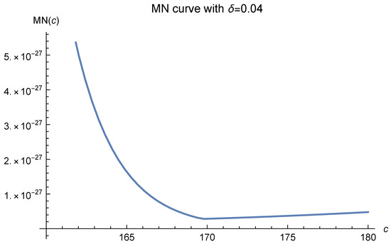
Figure 8. Here, $n=2,\lambda =2,\sigma =0.1,$ and $b_0=10\sqrt{2}$.

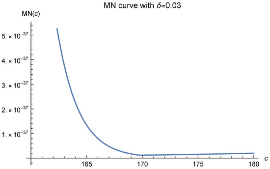
Figure 9. Here, $n=2,\lambda =2,\sigma =0.1,$ and $b_0=10\sqrt{2}$.

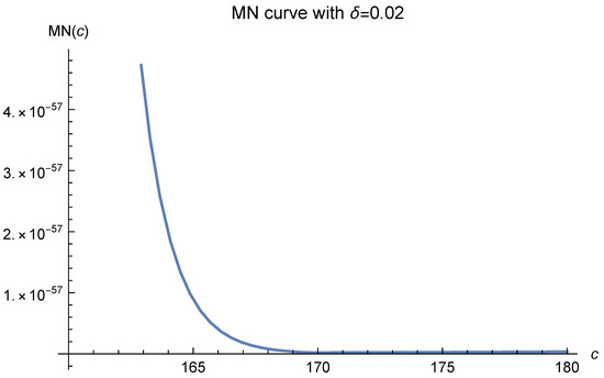
Figure 10. Here, $n=2,\lambda =2,\sigma =0.1,$ and $b_0=10\sqrt{2}$.

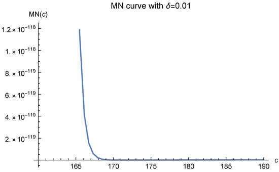
Figure 11. Here, $n=2,\lambda =2,\sigma =0.1,$ and $b_0=10\sqrt{2}$.

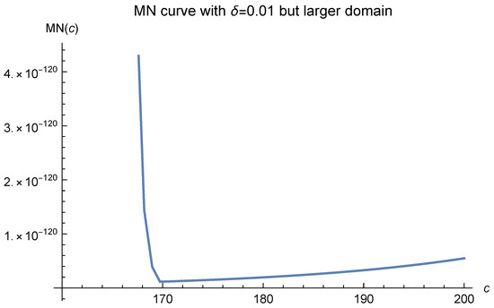
Figure 12. Here, $n=2,\lambda =2,\sigma =0.1,$ and $b_0=10\sqrt{2}$.

An immediate result of this phenomenon is that the experimentally optimal values of c may fall to the right of 170, especially when the curve is nearly horizontal there. The wider the nearly horizontal zone is, the farther the optimal value may fall to the right of 170.

This drawback will appear if we further increase the number $N=80$ of data points in Table 5, as shown in Table 6, Table 7, Table 8 and Table 9.

Table 6. $N=160,N_t=441$.

c	170	300	400 *	500	1000
RMS	$6.0\times {10}^{-24}$	$1.2\times {10}^{-24}$	$5.2\times {10}^{-25}$	$1.9\times {10}^{-24}$	$8.8\times {10}^{-24}$
COND	$1.9\times {10}^{62}$	$1.8\times {10}^{72}$	$3.4\times {10}^{76}$	$7.0\times {10}^{76}$	$1.4\times {10}^{90}$
c	2000	3000	5000
RMS	$1.7\times {10}^{-23}$	$1.8\times {10}^{-23}$	$1.9\times {10}^{-23}$
COND	$2.6\times {10}^{100}$	$2.7\times {10}^{106}$	$9.9\times {10}^{113}$

Table 7. $N=320,N_t=441$.

c	100	170	300	400	500
RMS	$1.3\times {10}^{-30}$	$7.9\times {10}^{-34}$	$1.1\times {10}^{-37}$	$2.9\times {10}^{-38}$	$2.7\times {10}^{-38}$
COND	$1.2\times {10}^{81}$	$1.9\times {10}^{92}$	$1.8\times {10}^{104}$	$2.1\times {10}^{110}$	$1.0\times {10}^{115}$
c	600 *	700	800	900	1000
RMS	$2.4\times {10}^{-38}$	$8.6\times {10}^{-38}$	$2.4\times {10}^{-37}$	$5.1\times {10}^{-37}$	$8.7\times {10}^{-37}$
COND	$7.2\times {10}^{118}$	$1.3\times {10}^{122}$	$8.3\times {10}^{124}$	$2.5\times {10}^{127}$	$4.1\times {10}^{129}$
c	2000	3000	5000
RMS	$5.1\times {10}^{-36}$	$7.6\times {10}^{-36}$	$9.6\times {10}^{-36}$
COND	$1.5\times {10}^{144}$	$5.0\times {10}^{152}$	$2.5\times {10}^{163}$

Table 8. $N=640,N_t=441$.

c	100	170	300	400	500
RMS	$8.9\times {10}^{-42}$	$9.2\times {10}^{-48}$	$1.2\times {10}^{-53}$	$7.8\times {10}^{-56}$	$1.9\times {10}^{-57}$
COND	$3.2\times {10}^{109}$	$2.9\times {10}^{125}$	$5.1\times {10}^{142}$	$3.0\times {10}^{151}$	$1.9\times {10}^{158}$
c	600	700 *	800	900	1000
RMS	$1.6\times {10}^{-58}$	$8.7\times {10}^{-59}$	$3.7\times {10}^{-58}$	$1.0\times {10}^{-57}$	$1.5\times {10}^{-57}$
COND	$6.8\times {10}^{163}$	$3.4\times {10}^{168}$	$4.0\times {10}^{172}$	$1.5\times {10}^{176}$	$4.1\times {10}^{177}$
c	2000	3000	5000
RMS	$1.9\times {10}^{-55}$	$3.3\times {10}^{-55}$	$6.6\times {10}^{-43}$
COND	$4.8\times {10}^{198}$	$1.0\times {10}^{211}$	$1.6\times {10}^{224}$

Table 9. $N=1280,N_t=441$.

c	100	170	300	400	500
RMS	$2.4\times {10}^{-59}$	$2.4\times {10}^{-69}$	$2.5\times {10}^{-78}$	$1.5\times {10}^{-82}$	$3.2\times {10}^{-85}$
COND	$6.5\times {10}^{152}$	$6.1\times {10}^{175}$	$2.2\times {10}^{200}$	$6.3\times {10}^{212}$	$2.8\times {10}^{222}$
c	600	700	800	900	1000 *
RMS	$7.7\times {10}^{-88}$	$4.6\times {10}^{-88}$	$6.6\times {10}^{-89}$	$2.2\times {10}^{-89}$	$2.0\times {10}^{-89}$
COND	$2.2\times {10}^{230}$	$9.8\times {10}^{236}$	$5.7\times {10}^{242}$	$7.0\times {10}^{247}$	$2.5\times {10}^{252}$
c	1100	1200	2000	3000	5000
RMS	$2.4\times {10}^{-89}$	$2.6\times {10}^{-89}$	$4.7\times {10}^{-86}$	$1.9\times {10}^{-84}$	$8.6\times {10}^{-82}$
COND	$3.2\times {10}^{256}$	$1.8\times {10}^{260}$	$1.9\times {10}^{282}$	$4.1\times {10}^{298}$	$8.1\times {10}^{320}$

This limitation does cause some trouble. Hence, one should carefully analyze the MN curves in advance when using this approach to find the optimal value of the shape parameter.

4. Discussion

Although we briefly mentioned the origin and significance of shifted surface splines in the Introduction, readers interested in this kind of radial basis function should refer to Dyn et al. [10,11,12] for a more detailed understanding.

In fact, each smooth (infinitely differentiable) radial basis function contains a shape parameter whose choice is always a substantial problem. The first theoretical work dealing with this question can be seen in Madych [13]. Although Madych could not effectively solve this question, his effort and intelligence are worthy of respect. In 1999 [14], Rippa introduced a trial-and-error algorithm to handle this problem. Then, Fasshauer, in his famous book [15], pointed out that only trial-and-error methods were available. Hence, how to theoretically predict the optimal value has been an open question in the field of RBFs (radial basis functions).

The function space $B_{\sigma }$ adopted in this paper is smaller than the space $E_{\sigma }$ adopted in Luh [1]. Hence, the error bound is sharper and leads to more accurate function interpolation. Another important property of $B_{\sigma }$ is that it serves as a bridge between Sobolev-space functions and radial basis functions (RBFs), as explained in the paragraph following Definition 1. Hence, we are now in the position to handle PDEs whose solutions lie in a Sobolev space.

5. Conclusions

In this paper, we successfully handled the problem of choosing the shape parameter optimally and totally discarded the traditional time-consuming trial-and-error methods. The optimal value of c can be directly predicted without a search. Hence, no algorithm is involved, and the time-consuming work of solving a linear system for each trial of the c value is completely avoided. The future challenge will probably be determining how to apply this approach to solve partial differential equations.

References

- Luh, L.-T. The Shape Parameter in the shifted surface Spline—An Easily Accessible Approach. Mathematics 2022, 10, 2844. [Google Scholar] [CrossRef]
- Abramowitz, M.; Segun, I.A. Handbook of Mathematical Functions; Dover Publications, Inc.: New York, NY, USA, 1970. [Google Scholar]
- Wendland, H. Scattered Data Approximation; Cambridge University Press: Cambridge, UK, 2005. [Google Scholar]
- Buhmann, M. Radial Basis Functions: Theory and Implementations; Cambridge University Press: Cambridge, UK, 2003. [Google Scholar]
- Madych, W.R.; Nelson, S.A. Multivariate Interpolation and Conditionally Positive Definite Function. Approx. Theory Appl. 1988, 4, 77–89. [Google Scholar] [CrossRef]
- Madych, W.R.; Nelson, S.A. Multivariate Interpolation and Conditionally Positive Definite Function, II. Math. Comp. 1990, 54, 211–230. [Google Scholar] [CrossRef]
- Luh, L.-T. The Mystery of the Shape Parameter III. Appl. Comput. Harmon. Anal. 2016, 40, 186–199. [Google Scholar] [CrossRef]
- Luh, L.-T. The Shape Parameter in the Shifted Surface Spline III. Eng. Anal. Boundary Elem. 2012, 36, 1604–1617. [Google Scholar] [CrossRef]
- Fleming, W. Functions of Several Variables, 2nd ed.; Springer: Berlin/Heidelberg, Germany, 1977. [Google Scholar]
- Dyn, N. Interpolation and Approximation by Radial and Related Functions; Approximation Theory VI; Chui, C.K., Schumaker, L.L., Ward, J., Eds.; Academic Press: Cambridge, MA, USA, 1989; pp. 211–234. [Google Scholar]
- Yoon, J. Approximation in Lp(Rd) from a Space Spanned by the Scattered Shifts of a Radial Basis Function. Constr. Approx. 2001, 17, 227–247. [Google Scholar] [CrossRef]
- Yoon, J. Lp Error Estimates for ‘Shifted’ Surface Spline Interpolation on Sobolev Space. Math. Comput. 2003, 243, 1349–1367. [Google Scholar]
- Madych, W.R. Miscellaneous Error Bounds for Multiquadric and Related Interpolators. Comput. Math. Appl. 1992, 24, 121–138. [Google Scholar] [CrossRef]
- Rippa, S. An algorithm for selecting a good value for the parameter c in a radial basis function interpolation. Adv. Comput. Math. 1999, 11, 193–210. [Google Scholar] [CrossRef]
- Fasshauer, G. Meshfree Approximation Methods with MATLAB; World Scientific Publishers: Singapore, 2007. [Google Scholar]
Disclaimer/Publisher’s Note: The statements, opinions and data contained in all publications are solely those of the individual author(s) and contributor(s) and not of MDPI and/or the editor(s). MDPI and/or the editor(s) disclaim responsibility for any injury to people or property resulting from any ideas, methods, instructions or products referred to in the content. |
© 2024 by the author. Licensee MDPI, Basel, Switzerland. This article is an open access article distributed under the terms and conditions of the Creative Commons Attribution (CC BY) license (https://creativecommons.org/licenses/by/4.0/).